Quantum Theory of Wave Scattering from Electromagnetic Time Interfaces
Modulating macroscopic parameters of materials in time reveals alternative avenues for manipulating electromagnetic waves. Due to such a significant impact, the general research subject of time-varying systems is flourishing today in different branches of electromagnetism and optics. However, besides uncovering different phenomena and effects in the realm of classical electrodynamics, we need to simultaneously study also the quantum aspects of this emerging subject in order to comprehend thoroughly the behavior of quanta of electromagnetic fields. Here, through the lens of quantum optics, we scrutinize the interaction of electromagnetic waves with materials whose effective parameters suddenly change in time. In particular, considering the basic case of temporal discontinuity for the refractive index of a non-dispersive dielectric material, we explicitly show the transformation of bosonic annihilation and creation operators and describe corresponding output quantum states for two specific input states: A Fock state and a coherent state. Accordingly, we rigorously elucidate the probability distribution and illustrate the related photon statistics. In consequence, we explain phenomena such as photon-pair generation and remark on several important conditions associated with photon statistics. Hopefully, this work paves the road for further vital explorations of a quantum theory of wave interaction with photonic time crystals or with dispersive time-varying materials.
1 Introduction
Investigation of wave interaction with materials where the effective material parameters vary in time is currently at the core of research in the electrodynamics community [1, 2]. This is because temporal variation renders an additional degree of freedom for controlling electromagnetic waves in a desired way [3, 4]. One of the basic scenarios within this area is to consider a temporal discontinuity according to which the effective parameters suddenly change from one value to another, although they are uniform in space [5]. In analogous to spatial discontinuity, this results in the emergence of reflected waves, and, in contrast, it gives rise to the frequency translation phenomenon and breaking the conservation of power [5, 6, 7]. Besides such important occurrences which were studied theoretically [5, 8, 6, 7] as well as experimentally [9, 10, 11, 12], other enticing effects have been reported. Indeed, by pondering temporal discontinuities in isotropic, anisotropic, and bianisotropic materials, various possibilities and effects have been uncovered including realization of dispersion bands separated by gaps in wavevector [13], anti-reflection temporal coatings [14, 15], inverse prism [16], temporal aiming [17], polarization conversion [18], polarization splitting [19], polarization-dependent analog computing [20], polarization rotation and direction-dependent wave manipulation [21], wave freezing and melting [22], transformation of surface waves into free-space radiation [23, 22], and so forth.
Beyond classical electrodynamics, the subject of temporal discontinuity in materials has engrossed attention also in quantum optics [24]. However, until today, such efforts are limited (see, e.g., Refs. [25, 26]) and not comparable with the ones that have been done in the realm of classical electrodynamics. Also, to the best of our knowledge, a comprehensive analysis that scrutinizes different aspects of the subject is missing, which is important for the future of this research direction. Thus, in this paper, we make the initial step and contemplate the wave interaction with temporal interfaces between two media from a quantum optics perspective. These two media are assumed to be dielectric and nondispersive. Accordingly, we derive the transformation of the bosonic operators and therefore rigorously calculate the final states when the initial ones are photon number states. In consequence, we elucidate the probability distribution and show several important conditions including the one under which the maximum probability of one photon-pair generation out of vacuum happens. In addition, we study the photon number fluctuations and demonstrate how temporal discontinuity engenders the creation of noise such that the reflected waves after the temporal discontinuity always follow super-Poissonian photon statistics. Furthermore, we revisit the above salient features when the initial states are coherent states rather than photon number states.
The paper is organized as follows: In Section 2, we briefly describe the problem of temporal discontinuity based on classical electromagnetics. This concise description is in fact needed to understand better what we explain in the next sections. In Section 3, which is the primary contribution of this paper, we study the problem from the quantum optics point of view as explained above. Finally, Section 4 concludes the paper and discusses our research objectives in this direction in the near future.
2 Classical Picture
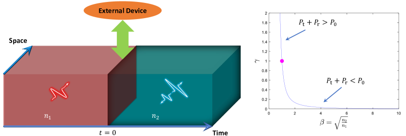
Consider an abrupt (step-like) change of refractive index in time. As shown in Fig. 1, there is a homogeneous nondispersive linear dielectric medium whose refractive index is denoted by before the temporal jump at and is represented by for . This kind of change called temporal discontinuity, temporal boundary, or time interface is in contrast to spatial boundary where the effective properties are discontinuous in space but uniform in time. For simplicity, we assume an initial uniform plane wave which is propagating in the -direction and is polarized along the -axis. Hence, regarding , the electric field is written as , where is the field amplitude, denotes the angular frequency, and is the corresponding wavevector component. Due to the presence of the time interface, we write the total field after as superposition of two plane waves with different amplitudes and angular frequencies. Accordingly, the electric field is given by
| (1) |
Since the medium does not vary in space, there is no reason that wavevector changes (conservation of ). With this fact, and, based on the dispersion relation
| (2) |
we conclude that
| (3) |
Note that and cannot be equal. Because the angular frequency becomes negative , it refers to a plane wave whose phase velocity is in the opposite direction compared to the one with positive angular frequency . Thus, these two plane waves correspond to the backward and forward waves. From a mathematical point of view, a plane wave with negative angular frequency and positive wavenumber is transferring energy in the positive-index medium quite similarly to a plane wave with positive angular frequency and negative wavenumber. This interesting characteristic enforces the postulation that the generated backward wave is in fact a reflected wave in space.
Having forward (transmitted) and backward (reflected) waves, technically, we can define transmission and reflection coefficients. For deriving them, similar to what we do concerning the spatial boundaries, we need boundary conditions. By observing Maxwell’s equations, we see that there are time derivatives of the electric and magnetic flux densities. Therefore, these two vectors should be continuous at the vicinity of when the refractive index abruptly increases or decreases. Therefore, we express the following important conditions:
| (4) |
It is crystal clear that if the medium does not have a magnetic response, the second term in the above equation means the continuity of the magnetic field (). In the case of locality in time, the electric flux density is connected to the electric field as , in which is the permittivity. As a result, using Eqs. (1) and (4), we infer that and , where by using Maxwell’s equations, the amplitudes of the magnetic field are given by , , and . Here, is the free-space intrinsic impedance. According to the above expressions, the reflection () and transmission () coefficients are eventually deduced as
| (5) |
Equation (5) indicates correctly that if , the reflection becomes zero, and we have full transmission.
Finally, it is worth mentioning about the conservation of power. In the case of having a spatial boundary, we know that the ratio between the summation of reflected and transmitted averaged power (per unit area) and the incident averaged power (per unit area) is unity. Indeed, , in which the reflection and transmission coefficients are identical with and [27]. Substituting these terms in the ratio, we obtain . However, for the time interface, we have a disparate story. If we generally calculate the ratio, we achieve that . By employing Eq. (5), the ratio equals to
| (6) |
that never goes to unity except that . Thus, regarding the time interface which we described, the conservation of power does not hold. This is because there is a pumping (or modulating) system which needs to do work in order to change the refractive index in time. Due to this work, the summation of the reflected and transmitted averaged power densities cannot be the same as the averaged power density associated with the initial wave propagating before . Notice that the ratio can be smaller or larger than unity depending on the refractive-index ratio, as shown by Eq. (6).
In summary, from the classical point of view, we succinctly explained the most salient features of temporal discontinuity that are angular frequency conversion (Eq. (3)), creation of reflected waves (Eq. (5)), and breaking conservation of power (Eq. (6)). Remembering these three properties which have been also illustrated by Fig. 1, in the following, we move to examine the quantum aspects of the problem.
3 Quantum Picture
This is the leading part of the study in which we are going to contemplate the scattering of electromagnetic waves from the proposed temporal interface based on employing the quantum optics paradigm. Hence, we will achieve a thorough understanding of the quanta of electromagnetic fields by describing the output quantum states and the related probability distribution as well as analyzing the photon statistics. Thus, as the first step, we deduce the output quantum states by assuming that the input state is in fact a Fock state that is sub-Poissonian and anti-bunched with zero variance for the number operator. Notice that at the end of the current section, we revisit our inspections for the case of a coherent state as the input one, and, therefore, we see the differences in output results corresponding to these two input states.
3.1 Output quantum states
We start by writing the electric field operator. Since the electromagnetic time interface causes the generation of reflected waves, we need to consider two modes that simultaneously exist before and after the temporal jump at . Consequently, by having such a consideration, the electric field operator is expressed as
| (7) |
Here, is the reduced Planck’s constant, and and denote the bosonic operators before and after , respectively. In fact, these bosonic operators are connected to each other via the electromagnetic boundary conditions which state that the flux density operators must be continuous at . In other words, quite similar to the classic picture, we have
| (8) |
The electric flux density is readily calculated because (we stress that this expression is valid only due to the temporal locality [28] which we initially postulated). However, to obtain the magnetic flux density, we use Faraday’s law in Maxwell’s equations which is . Afterward, by imposing those boundary conditions expressed in Eq. (8) and doing some algebraic manipulations, we conclude that
| (9) |
and
| (10) |
These equations demonstrate that temporal discontinuity is a transformation that relates the annihilation operator (creation operator ) to the annihilation (creation) and creation (annihilation) operators of the transmitted (reflected) and reflected (transmitted) waves, respectively. To better understand these relations, the first term is denoted by , and the second term is represented by . Hence, Eq. (9) is reduced to and . Interestingly, contemplating these coefficients and , we see that and . In other words, is inverse of , which results in
| (11) |
First, this relation allows us to achieve the following commutation relation as . Second, more importantly, based on trigonometric functions, we know that , and, based on hyperbolic functions, we have a similar relation but with a minus sign: . Thus, Eq. (11) manifests that we can make and equivalent to the hyperbolic functions and , respectively (i.e., and ). Due to such an equivalence, we rewrite Eq. (9) as
| (12) |
It is crystal clear that the square matrix in Eq. (12) is a Hermitian transformation matrix that in this form maps the operators to . While the corresponding determinant is unity, we see that the matrix is not unitary. However, we will show how this non-unitary matrix results in deriving the output quantum states. For that, first, we propound a unitary operator denoted as and given by . Concerning this operator, we infer that and . These expressions are deduced by employing the general relation that as well as by using the Taylor series of hyperbolic functions (i.e., and ). Considering Eq. (12) and the above expressions together give rise to a paramount conclusion that
| (13) |
In other words, is the unitary transformation of , and, accordingly, can be represented as a unitary evolution operator: , where and . Thus, the output quantum state is achieved by applying the operator to the initial state. Here, let us suppose that this initial state is a Fock state . This means that one mode consists of photons, and the other mode corresponds to the ground level. Before continuing, two points are worth mentioning. The first one is that since the operator consists of the operators, and we are going to apply it to , we need to consider the inverse of the matrix expressed in Eq. (12) so that . By doing such task, we see that explicitly ). This is the intriguing characteristic of the transformation matrix in Eq. (12). The second point is that because the operator is in the form of an exponential, it is convenient to employ disentanglement theorem [29], which allows us to re-write the operator as
| (14) |
where , , and , in which the operators obey the following commutation relations: and . Having the above equation and using the Taylor expansion that , we ultimately derive the final state which is associated with the new medium after the temporal jump (recall that ).
In Eq. (14), there are three terms. The last term (i.e., ) is useless, because it is about annihilation operators, and we already assumed that the second mode is in the ground level. Regarding the middle term, we obtain that
| (15) |
In other words, is the eigenvalue of the operator of the middle term with the eigenstate . In consequence, we observe that the last and middle terms do not change the state, and is conserved. However, the situation is drastically different for the first term because it includes the creation operators. Indeed, if we apply the basic relations of quantum mechanics that and , we infer the output state which is expressed as
| (16) |
This equation explicitly demonstrates that the first term in Eq. (14) causes excitation of higher energy levels, and is only part of a distribution that contributes with the probability of .
3.2 Probability distribution
According to Eq. (16), we achieve a probability-distribution function which is given by
| (17) |
This probability function can be rewritten based on the coefficients and . In fact, since and , we deduce that . From the theory of series, we know that for . Replacing by and using the aforementioned identity, we indicate that the summation of with respect to the integer is unity. In other words, we prove that , which is considered as a sanity check. To start contemplating Eq. (17), we inspect the scenario in which the initial state is a vacuum state, and there is no photon . Accordingly, the above expression is reduced to
| (18) |
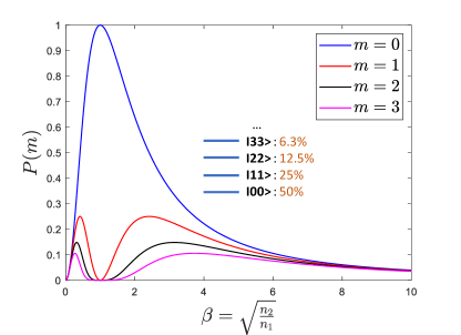
where is the square root of the ratio of the refractive indexes. First, we observe from Eq. (18) that the probability of remaining in the vacuum state after the temporal jump is . This means that when (which corresponds to changing to zero-index materials or low-index materials compared to the initial medium), or when is very large (jumping to high-index materials), such possibility is negligible. Second, on the other hand, the above equation indicates that there is the possibility of generating photon pairs from the initial vacuum. In fact, for creating one photon pair (), the corresponding probability equals to . Definitely, this probability is smaller than the one for the vacuum state (). However, for specific values of , it becomes maximum. To find those values, we need to see where the derivative with respect to vanishes. After some algebraic manipulations, we achieve that or . In this scenario, the probability of generating one photon pair is maximally 25 for both positive and negative signs. If we substitute these particular values of in the equation for the probability of vacuum state, it is shown that 50% we have a chance to keep the vacuum state (regardless of those signs). And, certainly, we have a 25% chance to obtain higher amounts of photon pairs. These results are shown in Fig. 2 in which the probability function described by Eq. (18) is shown concerning the state number and as the ratio between the indexes. This figure illustrates that at , the function , and it is zero for , as we expect. It also shows that when the value of is large enough, the probability distribution becomes more uniform regarding different excited states. Indeed, if , Eq. (18) is reduced to confirming that the probability function becomes independent from the value of .
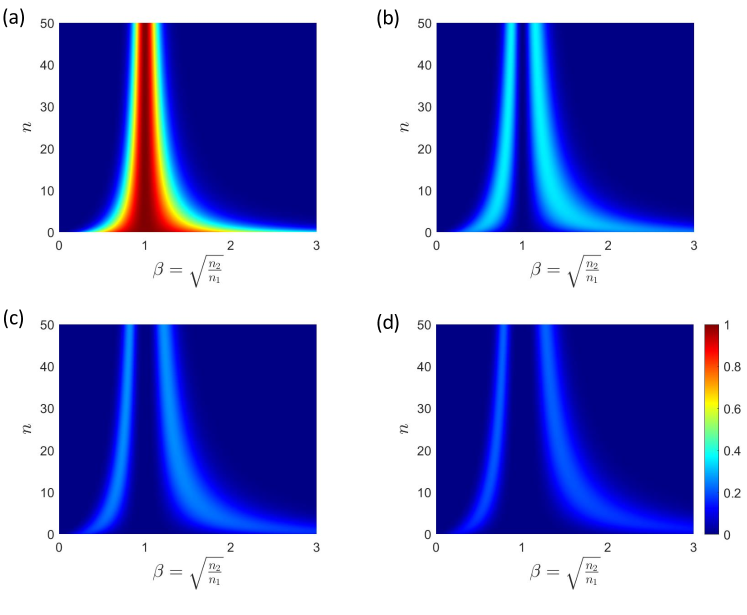
The probability distribution with respect to and for several values of is presented in Fig. 3. Based on this figure, we see that the probability of the state is high when the value of is close to unity. As diverges from unity, this probability decreases. However, we observe that the probability of generating a photon pair is enhanced. Regarding only one photon pair generation, the figure illustrates that there is the possibility of 35% to achieve . In this case,
| (19) |
We simply find the maximum probability for a given by taking the derivative of zero. Accordingly, we deduce that which results in . The lower limit is which is associated with as we discussed before, and the upper limit that corresponds to high values of is (recall that when approaches zero). Note that there are points at which the probability of one-, two-, or three-pair photon generation is higher than the probability related to .
3.3 Photon number fluctuations
Next, we contemplate photon statistics of forward and backward modes by studying expectation value and variance of the corresponding number operators. We define those number operators as and . Employing Eq. (12), we obtain the following transformation
| (20) |
and write that
| (21) |
We supposed that the second mode before the temporal jump is in the ground state (vacuum state). Having this condition and using Eq. (21), the expectation values of the above number operators are simplified and reduced to and . Since before , we have photons that are carried by the first mode, therefore, the difference in the average number of photons after and before the temporal discontinuity equals to
| (22) |
This equation illustrates that under the condition of , on average, we generate a single photon. This condition can be represented in terms of the refractive indexes. In fact, it gives rise to . For instance, if the initial number of photons is zero (), the refractive index of the medium after should be times the refractive index corresponding to the initial medium.
By having the expectation values, we do some algebraic manipulations to determine the expectation values of the square of the number operators, and, thus, calculate the photon number fluctuations (). In accordance, we deduce that
| (23) |
We did not mention the derivations related to for the shortness. Equation (23) preliminarily shows that the temporal discontinuity of the refractive index engenders photon number fluctuations, although those fluctuations vanish before the refractive index jumps in time. Furthermore, more importantly, we explicitly observe that since , for the second mode (, ), the variance is always larger than the expectation value. Hence, this mode corresponds to a super-Poissonian wave. However, the scenario is apparently different for the first mode (, ). In fact, Eq. (23) indicates that the variance can be larger or smaller than the expectation value due to the possible values of . Accordingly, it means that the generated forward wave after the temporal jump is classified as a sub-Poissonian or super-Poissonian wave depending on the ratio parameter . By using Eq. (23) and applying that , the condition for having a super-Poissonian transformation is obtained as
| (24) |
Based on the above expressions, we see that if the initial number of photons is considerable (), the aforementioned conditions are simplified to and which mean that or . Intriguingly, on the opposite case, if the initial photon number is zero (), Eq. (24) states that the forward wave is always super-Poissonian regardless of the ratio parameter .
3.4 Degree of second-order coherence
After determining the photon number fluctuations, it is sensible to calculate the degree of second-order coherence that is given by . This calculation helps to assess the forward and backward waves after the temporal discontinuity and see if they are bunched or anti-bunched waves. Recall that for coherent states, is unity. Thus, the waves with larger than unity are called bunched waves, and the waves with are coined anti-bunched waves [30].
In the previous part, we derived the expectation values and variances for those waves after . Thus, we readily obtain the corresponding expressions for the function. Thus, we infer that
| (25) |
First, we explicitly see that the function does not depend on the variable for the backward wave. It is a function of only . Second, Eq. (25) indicates that this wave is always bunched, and its degree of second-order coherence varies between one () and two (). However, concerning the forward wave, we see that it is strongly dependent on both and . In fact, if , we achieve as expected, because corresponds to vanishing the temporal discontinuity. On the other hand, if tends to infinity, the degree equals which is larger than unity. Thus, there is a particular point at which the function becomes unity. Before and after this point, the forward wave is anti-bunched and bunched, respectively. By using Eq. (25), interestingly, we deduce exactly the same conditions that were described before by Eq. (24). This is consistent with the conventional scenarios. In other words, anti-bunched waves are sub-Poissonian, and bunched waves are super-Poissonian. Notice that we summarized all these enticing conclusions about photon statistics in Table 1.
| Photon Statistics | |||
|---|---|---|---|
| Input State | Output Mode | Photon Number Fluctuations | Degree of Second-order Coherence |
| Number State | Backward Wave | Super-Poissonian | Bunched |
| Number State | Forward Wave | Super-Poissonian () | Bunched () |
| Number State | Forward Wave | Sub-Poissonian () | Anti-Bunched () |
| Coherent State | Backward Wave | Super-Poissonian | Bunched |
| Coherent State | Forward Wave | Super-Poissonian | Bunched |
3.5 Coherent states
In the previous parts, we studied the photon number states. Here, we concisely contemplate the scenario that the forward wave before the temporal discontinuity is a coherent state described as
| (26) |
in which is the eigenvalue regarding the annihilation operator. Since the number operator corresponding to the forward and backward waves is represented by the bosonic annihilation and creation operators before the temporal jump (see Eq. (21)), it is straightforward to derive the expectation values. After some algebraic manipulations, the expectation value of the number operator for the forward and backward wave is achieved as and , respectively. In analogy with what we did for the photon number states, we will calculate the difference between the expectation values before and after the temporal jump and interestingly attain the same expression. Indeed, we prove that , which is similar to Eq. (22).
Afterward, we deduce the variance for the number operators. This determines if there are fluctuations as well as the class of the created waves (i.e., sub-Poissonian or super-Poissonian). Recall that the coherent states are associated with Poissonian distribution because the variance is equal to the mean value. However, as we observed for photon number states, the temporal discontinuity may drastically change the situation. By doing the required calculations, we infer that
| (27) |
Comparing these results with the ones we achieved for photon number states, we see that unlike Eq. (23), the variances for the forward and backward modes are not the same (). There is a difference which equals to . Notice that the backward mode is again a super-Poissonian wave because , and, consequently, the corresponding variance is larger than the expectation value. Concerning the forward mode, initially, we may think that similar to the photon number state, it can be sub- or super-Poissonian because the expression inside the parentheses in Eq. (27) is multiplied by which can be zero. However, as approaches zero, the expression inside the parentheses tends to infinity. By taking a limit, it is seen that in this case, the variance approaches . If we divide the variance by the expectation value and take the limit, we see that
| (28) |
which claims that the forward wave is also following super-Poissonian photon statistics.
Similarly to what we did for the photon number states, here, we deduce the degree of second-order coherence when the input state is in fact a coherent state. Having the expectation values and the variances, we derive that
| (29) |
Akin to the input number state, we observe that the for the backward wave is dependent on only the absolute value of while for the forward wave, it is a function of the square of as well. More importantly, in contrast to the input number state, these results in Eq. (29) explicitly demonstrate that for both forward and backward waves, the function is always larger than one, which means that both waves are associated with bunched waves. Remember that for the input number state, the forward wave under some conditions could be anti-bunched as illustrated by Table 1.
4 Conclusions
First, from a classical electrodynamics point of view, we briefly reviewed the main features of wave scattering from time interfaces. Subsequently, as the principal aim, we thoroughly studied the problem from a quantum optics perspective. Accordingly, we inspected the transformation of bosonic operators due to the existence of temporal discontinuity in the refractive index and calculated the states as the result of such transformation. Taking the Fock states as granted before , we observed that photon-pair generation is at the heart of this transformation. We contemplated the probability distribution and analyzed the conditions of creating one-photon pair with maximum probability. In addition, for two input states, Fock states and coherent states, we scrutinized photon number fluctuations and the degree of second-order coherence to assess photon statistics. We see that the backward mode is always super-Poissonian (bunched) after , while for the Fock states unlike coherent states, the forward mode can be sub-Poissonian (anti-bunched). Furthermore, we found also the condition to create a single photon on average after the temporal jump at .
As we remarked earlier, this scrutiny is our initial but foundational step for the future. Through the lens of classical electrodynamics, we know that if the dielectric medium under study becomes dispersive, and temporal nonlocality plays a role, the time interface results in the generation of at least two angular frequencies after , in contrast to the nondispersive scenario. From a quantum optics point of view, this has a significant impact and opens new possibilities which need to be carefully examined. Thus, we are interested in expanding the current study shortly by taking the dispersion into account. Also, as can be expected, one enticing problem as the next step is to investigate temporal slabs so that we give a rigorous quantum theory of wave interaction with materials whose corresponding band structure shows wavevector bandgaps due to the periodic modulation of the refractive index.
Acknowledgment
This work was supported by the Research Council of Finland (Grants Nos. 354918, 346518, 349396, and 336119).
References
- [1] E. Galiffi, R. Tirole, S. Yin, H. Li, S. Vezzoli, P. A. Huidobro, M. G. Silveirinha, R. Sapienza, A. Alù, and J. Pendry, “Photonics of time-varying media,” Advanced Photonics, vol. 4, no. 1, pp. 014 002–014 002, 2022.
- [2] G. Ptitcyn, M. S. Mirmoosa, A. Sotoodehfar, and S. A. Tretyakov, “A tutorial on the basics of time-varying electromagnetic systems and circuits: Historic overview and basic concepts of time-modulation.” IEEE Antennas and Propagation Magazine, 2023.
- [3] N. Engheta, “Four-dimensional optics using time-varying metamaterials,” Science, vol. 379, no. 6638, pp. 1190–1191, 2023.
- [4] ——, “Metamaterials with high degrees of freedom: space, time, and more,” Nanophotonics, vol. 10, no. 1, pp. 639–642, 2021.
- [5] F. R. Morgenthaler, “Velocity modulation of electromagnetic waves,” IRE Transactions on Microwave Theory and Techniques, vol. 6, no. 2, pp. 167–172, 1958.
- [6] J. Mendonça and P. Shukla, “Time refraction and time reflection: two basic concepts,” Physica Scripta, vol. 65, no. 2, p. 160, 2002.
- [7] Y. Xiao, D. N. Maywar, and G. P. Agrawal, “Reflection and transmission of electromagnetic waves at a temporal boundary,” Optics letters, vol. 39, no. 3, pp. 574–577, 2014.
- [8] S. C. Wilks, J. M. Dawson, and W. B. Mori, “Frequency up-conversion of electromagnetic radiation with use of an overdense plasma,” Phys. Rev. Lett., vol. 61, pp. 337–340, Jul 1988.
- [9] N. Yugami, T. Niiyama, T. Higashiguchi, H. Gao, S. Sasaki, H. Ito, and Y. Nishida, “Experimental observation of short-pulse upshifted frequency microwaves from a laser-created overdense plasma,” Phys. Rev. E, vol. 65, p. 036505, Mar 2002.
- [10] A. Nishida, N. Yugami, T. Higashiguchi, T. Otsuka, F. Suzuki, M. Nakata, Y. Sentoku, and R. Kodama, “Experimental observation of frequency up-conversion by flash ionization,” Applied Physics Letters, vol. 101, no. 16, 2012.
- [11] V. Bacot, M. Labousse, A. Eddi, M. Fink, and E. Fort, “Time reversal and holography with spacetime transformations,” Nature Physics, vol. 12, pp. 972–977, 2016.
- [12] H. Moussa, G. Xu, S. Yin, E. Galiffi, Y. Ra’di, and A. Alù, “Observation of temporal reflection and broadband frequency translation at photonic time interfaces,” Nature Physics, vol. 19, pp. 863–868, 2023.
- [13] E. Lustig, Y. Sharabi, and M. Segev, “Topological aspects of photonic time crystals,” Optica, vol. 5, no. 11, pp. 1390–1395, 2018.
- [14] D. Ramaccia, A. Toscano, and F. Bilotti, “Light propagation through metamaterial temporal slabs: reflection, refraction, and special cases,” Optics Letters, vol. 45, no. 20, pp. 5836–5839, 2020.
- [15] V. Pacheco-Peña and N. Engheta, “Antireflection temporal coatings,” Optica, vol. 7, no. 4, pp. 323–331, 2020.
- [16] A. Akbarzadeh, N. Chamanara, and C. Caloz, “Inverse prism based on temporal discontinuity and spatial dispersion,” Optics Letters, vol. 43, no. 14, pp. 3297–3300, 2018.
- [17] V. Pacheco-Peña and N. Engheta, “Temporal aiming,” Light: Science & Applications, vol. 9, no. 1, p. 129, 2020.
- [18] J. Xu, W. Mai, and D. H. Werner, “Complete polarization conversion using anisotropic temporal slabs,” Optics Letters, vol. 46, no. 6, pp. 1373–1376, 2021.
- [19] M. H. M. Mostafa, M. S. Mirmoosa, and S. A. Tretyakov, “Spin-dependent phenomena at chiral temporal interfaces,” Nanophotonics, vol. 12, no. 14, pp. 2881–2889, 2023.
- [20] C. Rizza, G. Castaldi, and V. Galdi, “Spin-controlled photonics via temporal anisotropy,” Nanophotonics, vol. 12, no. 14, pp. 2891–2904, 2023.
- [21] M. S. Mirmoosa, M. H. Mostafa, A. Norrman, and S. A. Tretyakov, “Time interfaces in bianisotropic media,” arXiv:2306.17522, 2023.
- [22] X. Wang, M. S. Mirmoosa, and S. A. Tretyakov, “Controlling surface waves with temporal discontinuities of metasurfaces,” Nanophotonics, vol. 12, no. 14, pp. 2813–2822, 2023.
- [23] A. V. Shirokova, A. V. Maslov, and M. I. Bakunov, “Scattering of surface plasmons on graphene by abrupt free-carrier generation,” Phys. Rev. B, vol. 100, p. 045424, Jul 2019.
- [24] J. Mendonça, A. Guerreiro, and A. M. Martins, “Quantum theory of time refraction,” Physical Review A, vol. 62, no. 3, p. 033805, 2000.
- [25] J. E. Vázquez-Lozano and I. Liberal, “Shaping the quantum vacuum with anisotropic temporal boundaries,” Nanophotonics, vol. 12, no. 3, pp. 539–548, 2022.
- [26] I. Liberal, J. E. Vázquez-Lozano, and V. Pacheco-Peña, “Quantum antireflection temporal coatings: quantum state frequency shifting and inhibited thermal noise amplification,” Laser & Photonics Reviews, vol. 17, no. 9, p. 2200720, 2023.
- [27] D. K. Cheng et al., Field and wave electromagnetics. Pearson Education India, 1989.
- [28] M. Mirmoosa, T. Koutserimpas, G. Ptitcyn, S. Tretyakov, and R. Fleury, “Dipole polarizability of time-varying particles,” New Journal of Physics, vol. 24, no. 6, p. 063004, 2022.
- [29] K. Wodkiewicz and J. Eberly, “Coherent states, squeezed fluctuations, and the su(2) and su(1, 1) groups in quantum-optics applications,” JOSA B, vol. 2, no. 3, pp. 458–466, 1985.
- [30] A. M. Fox, Quantum optics: an introduction. Oxford University Press, USA, 2006, vol. 15.