Stochastic Data-Driven Predictive Control
with Equivalence to Stochastic MPC

Abstract

We propose a data-driven receding-horizon control method dealing with the chance-constrained output-tracking problem of unknown stochastic linear time-invariant (LTI) systems with partial state observation. The proposed method takes into account the statistics of the process noise, the measurement noise and the uncertain initial condition, following an analogous framework to Stochastic Model Predictive Control (SMPC), but does not rely on the use of a parametric system model. As such, our receding-horizon algorithm produces a sequence of closed-loop control policies for predicted time steps, as opposed to a sequence of open-loop control actions. Under certain conditions, we establish that our proposed data-driven control method produces identical control inputs as that produced by the associated model-based SMPC. Simulation results on a grid-connected power converter are provided to illustrate the performance benefits of our methodology.

1 Introduction

Model predictive control (MPC) is a widely used multi-variable control technique [1], capable of handling hard constraints on inputs, states, and outputs, along with complex performance criteria. Constraints can model actuator saturations or encode safety constraints in safety-critical applications. As the name suggests, MPC uses a system model, obtained either from first-principles modelling or from identification, to predict how inputs will influence the system evolution. MPC is therefore an indirect design method, since one goes from data to a controller through an intermediate modelling step [2]. In contrast, direct methods, or data-driven methods, seek to compute controllers directly from input-output data. Data-driven methods show promise for systems that are complex or difficult to model [3].

For stochastic systems, work on Stochastic MPC (SMPC) [4, 5, 6] has focused on modelling the uncertainty in systems probabilistically. SMPC methods optimize over feedback control policies rather than control actions, resulting in performance benefits when compared to the naive use of deterministic MPC [7]. Additionally, SMPC allows the use of probabilistic constraints, useful for computing risk-aware controllers. Another MPC method dealing with uncertainty is Robust MPC (RMPC) [8], which attempts to conservatively guard against the worst-case deterministic uncertainty; our focus here is on the stochastic case.

For deterministic linear time-invariant (LTI) systems, recent work has demonstrated that the data-driven control methods can produce controls that are equivalent to their model-based counterparts [9, 10]. However, for stochastic systems, equivalence between a data-based and model-based method have not been established, except in a few special cases which will be discussed shortly. Thus, the focus of this work is to develop a data-driven stochastic MPC framework with provable equivalence to its model-based SMPC counterpart.

Related Work: Although data-driven control has been developed for decades, early work on data-driven methods did not adequately account for constraints on input and output; see examples in [3]. This observation led to the development of Data-Driven Predictive Control (DDPC) as data-driven control methods incorporating input and output constraints. Two of the best known DDPC methods are Data-Enabled Predictive Control (DeePC) [10, 11, 12] and Subspace Predictive Control (SPC) [13, 14], both of which have been applied in multiple experiments with reliable results [15, 16, 17, 18, 19, 20]. On the theoretical side, for deterministic LTI systems, both DeePC and SPC produce equivalent control actions to model-based MPC [10, 21]. This equivalence implies that for deterministic systems, DeePC and SPC perform as well as their model-based counterpart, namely MPC.

Beyond the idealized case with deterministic linear systems, real-world systems are often stochastic and non-linear, and real-life data typically are perturbed by noise. Hence, data-driven methods in practice need to adapt to data that is subject to these perturbations. Most classical data-driven control methods are designed in robust ways [3], so their control performances are not sensitive to noisy data. In application of SPC with noisy data, a predictor matrix is often computed with denoising methods, such as prediction error methods [18, 19] and truncated singular value decomposition [16].

Robust versions of DeePC have also been developed with stochastic systems in mind, such as norm-based regularized DeePC [15, 16, 17, 18, 19, 20] in which the regularization can be interpreted as a result of worst-case robust optimization [22, 23], as well as distributionally robust DeePC [11, 12]. Some other variations of DeePC were designed in purpose of ensuring closed-loop stability [24, 25, 26], robustness to nonlinear systems [27] etc. Although the stochastic adaptations of DeePC and SPC were validated through experiments, these stochastic data-driven methods do not possess an analogous theoretical equivalence to any Stochastic MPC or model-based method.

This disconnect between data-driven and model-based methods in the stochastic case has been noticed by some researchers, and some recent DDPC methods were developed for stochastic systems that have provable equivalence to model-based MPC methods. The works in [28, 29] proposed a data-driven control framework for stochastic systems with full-state observation, and their control method has equivalent performance to full-state-observation SMPC [28, Thm. 1] [29, Cor. 1]. This data-driven control method applied Polynomial Chaos Expansion, so that arbitrary probability distributions of stochastic signals can be considered. However, their formulation was built with full-state observation, and the partial observation case was left open.

In [30], a stochastic data-driven control method was developed by estimating the innovation sequence. This method has equivalent control performance to deterministic MPC when the innovation data is exact [30, Cor. 1]. However, their control method did not utilize the noise distribution, and no equivalence is established between their method and SMPC or RMPC. A final related work is [31], which proposed a tube-based data-driven Stochastic MPC framework with full-state observation. Again, however, no equivalence in performance is established between this method and model-based MPC methods. Thus, the gap addressed in this paper is to develop a data-driven control method for partially observed stochastic systems that has provably equivalent performance to the model-based SMPC.

Contributions: We develop a DDPC control method for stochastic LTI systems with partial state observation. Our technical approach is based on the construction of an auxiliary state model directly parameterized by input-output data. Building on SMPC, we formulate a stochastic control problem using this data-based auxiliary model, and establish equivalence between the proposed data-driven approach and its model-based SMPC counterpart. Our approach preserves three key features and benefits of SMPC. First, our formulation includes both process noise and measurement noise, so one can study the effect of different noise magnitudes on the control performance. Second, we produce a feedback control policy at each time step, so that the control inputs are decided after real-time measurements in a closed-loop manner. Third, our control method incorporates safety chance constraints, which are consistent with the SMPC framework that we investigate.

Organization: The rest of the paper is organized as follows. Section 2 shows the formal problem statement, with a brief overview of SMPC in Subsection 2.1. Our control method is introduced in Section 3, where we show the formulation and the theoretical performance guarantee, i.e., equivalence to SMPC. Simulation results are displayed in Section 4, comparing our proposed method and some benchmark control methods, and Section 5 is the conclusion.

Notation: Let $M^{\dagger}$ be the pseudo-inverse of a matrix $M$. Let $\otimes$ denote the Kronecker product. Let $\mathbb{S}^{q}_{+}$ and $\mathbb{S}^{q}_{++}$ be the sets of $q\times q$ positive semi-definite and positive definite matrices respectively. Let $\mathrm{col}(M_{1},\ldots,M_{k})$ denote the column concatenation of matrices/vectors $M_{1},\ldots,M_{k}$. Let $\mathbb{Z}_{[a,b]}:=[a,b]\cap\mathbb{Z}$ denote a set of consecutive integers from $a$ to $b$. Let $\mathbb{Z}_{[a,b)}:=\mathbb{Z}_{[a,b-1]}$. For a ^q-valued discrete-time signal $z_{t}$ with integer index $t$, let $z_{[t_{1},t_{2}]}$ denote either a sequence $\{z_{t}\}_{t=t_{1}}^{t_{2}}$ or a concatenated vector $\mathrm{col}(z_{1},\ldots,z_{2})\in{}^{q(t_{2}-t_{1}+1)}$. Similarly, let $z_{[t_{1},t_{2})}:=z_{[t_{1},t_{2}-1]}$. A matrix sequence $\{M_{t}\}_{t=t_{1}}^{t_{2}}$ and a function sequence $\{\pi_{t}(\cdot)\}_{t=t_{1}}^{t_{2}}$ are denoted by $M_{[t_{1},t_{2}]}$ and $\pi_{[t_{1},t_{2}]}$ respectively.

2 Problem Statement

We consider a stochastic linear time-invariant (LTI) system

$$x_{t+1}= \;Ax_{t}+Bu_{t}+w_{t}$$ (1a)

$$y_{t}= \;Cx_{t}+v_{t}$$ (1b)

with input $u_{t}\in{}^{m}$, state $x_{t}\in{}^{n}$, output $y_{t}\in{}^{p}$, process noise $w_{t}\in{}^{n}$, and measurement noise $v_{t}\in{}^{p}$. The initial state $x_{0}$ is unknown. The system $(A,B,C)$ is assumed to be a minimal realization, but the matrices themselves are unknown and the state $x_{t}$ is unmeasured; we have access only to the input $u_{t}$ and output $y_{t}$ in (1). The disturbances $w_{t}$ and $v_{t}$ in (1) are independent and follow i.i.d. zero-mean normal distributions, with variances $\Sigma^{\sf w}\in\mathbb{S}^{n}_{+}$ and $\Sigma^{\sf v}\in\mathbb{S}^{n}_{++}$ respectively, i.e.,

$$w_{t}\overset{\rm i.i.d}{\sim}\mathcal{N}(0_{n\times 1},\Sigma^{\sf w}),\quad v_{t}\overset{\rm i.i.d}{\sim}\mathcal{N}(0_{p\times 1},\Sigma^{\sf v}).$$ (2)

In a reference tracking problem, the objective is for the output $y_{t}$ to follow a specified reference signal $r_{t}\in{}^{p}$. The trade-off between tracking error and control effort may be encoded in the cost

$$J(u_{t},y_{t}):=\|y_{t}-r_{t}\|_{Q}^{2}+\|u_{t}\|_{R}^{2}$$ (3)

to be minimized over a horizon, where $Q\in\mathbb{S}^{p}_{++}$ and $R\in\mathbb{S}^{m}_{++}$ are user-selected parameters. This tracking should be achieved subject to constraints on the inputs and outputs. We consider polytopic constraints, modelled in the stochastic setting as probabilistic chance constraints for $t\in\mathbb{N}_{\geq 0}$,

$$\mathbb{P}\big{[}E^{\sf u}u_{t}\leq f^{\sf u}\big{]}\geq 1-p^{\sf u}$$ (4a)

$$\mathbb{P}\big{[}E^{\sf y}y_{t}\leq f^{\sf y}\big{]}\geq 1-p^{\sf y}$$ (4b)

where $E^{\sf u}\in{}^{q^{\sf u}\times m}$ and $E^{\sf y}\in{}^{q^{\sf y}\times m}$ are fixed matrices with some $q^{\sf u},q^{\sf y}\in\mathbb{N}$, $f^{\sf u}\in{}^{q^{\sf u}}$ and $f^{\sf y}\in{}^{q^{\sf y}}$ are fixed vectors, and $p^{\sf u},p^{\sf y}\in(0,1)$ are probabilities of constraint violation.

In a model-based setting where $A,B,C$ are known, the general control problem above can be addressed by SMPC, as will be reviewed in Section 2.1. Our broad objective is to construct a data-driven method that addresses the same stochastic control problem and is equivalent, under certain tuning conditions, to SMPC.

Remark 1 (Output Constraints and Output Tracking).

State constraints and state-tracking costs are commonly considered in MPC and SMPC methods [1, 4, 5, 6], being used to enforce safety conditions and quantify control performance, respectively. Our problem setup focuses on output control, with the internal state being unknown and unmeasured. For this reason, we instead considered output constraint (4b) for safety conditions and output-tracking cost (3) for performance evaluation, which are both common in DDPC methods such as [10].  

2.1 Stochastic MPC: A Benchmark Model-Based Design

Our focus is on output-feedback SMPC [32, 33, 34, 35, 36], which is typically approached by enforcing a separation principle within the design, augmenting full-state-feedback SMPC (see [4, Table 2]) with state estimation. Several formulations of SMPC methods have been developed in the literature; our formulation here is based on an affine policy parameterization, following e.g., [34] and those listed in [4, Table 2], with the changes that we consider output tracking and output constraint satisfaction, as opposed to state objectives.

SMPC follows a receding-horizon strategy and makes decisions for $N$ upcoming steps at each control step. At control step $t=k$, the current state $x_{k}$ follows a normal prior distribution

$$x_{k}\;\sim\;\mathcal{N}(\mu^{\sf x}_{k},\Sigma^{\sf x}_{k})$$ (5)

where the mean $\mu^{\sf x}_{k}\in{}^{n}$ and the variance $\Sigma^{\sf x}_{k}\in\mathbb{S}^{n}_{+}$ are parameters obtained through a Kalman filter to be described next. At the initial time $k=0$, the initial state $x_{0}\sim\mathcal{N}(\mu^{\sf x}_{0},\Sigma^{\sf x}_{0})$ is assumed to follow a normal distribution with a given mean $\mu^{\sf x}_{0}$ and a given variance $\Sigma^{\sf x}_{0}$. The model-based SMPC method under consideration combines state estimation, affine feedback policy parameterization, and approximation of chance constraints.

2.1.1 State Estimation

Estimates $\hat{x}_{[k,k+N)}$ of the future states over the desired horizon will be computed through the Kalman filter [34, 35, 36],

$$\hat{x}_{t} :=\hat{x}^{\scalebox{1.2}[1.0]{-}}_{t}+L_{t}(y_{t}-C\hat{x}^{\scalebox{1.2}[1.0]{-}}_{t}), t\in\mathbb{Z}_{[k,k+N)}$$ (6a)

$$\hat{x}^{\scalebox{1.2}[1.0]{-}}_{t+1} :=A\hat{x}_{t}+Bu_{t}, t\in\mathbb{Z}_{[k,k+N)}$$ (6b)

$$\hat{x}^{\scalebox{1.2}[1.0]{-}}_{k} :=\mu^{\sf x}_{k}$$ (6c)

where $\hat{x}_{t}$ and $\hat{x}_{t}^{\scalebox{1.2}[1.0]{-}}$ denote the posterior and prior estimates of $x_{t}$, respectively, and the Kalman gain $L_{t}\in{}^{n\times p}$ in (6a) is obtained via the recursion

$$L_{t} :=P^{\scalebox{1.2}[1.0]{-}}_{t}C^{\sf T}(CP^{\scalebox{1.2}[1.0]{-}}_{t}C^{\sf T}+\Sigma^{\sf v})^{-1}, t\in\mathbb{Z}_{[k,k+N)}$$ (7a)

$$P_{t} :=(I_{n}-L_{t}C)P^{\scalebox{1.2}[1.0]{-}}_{t}, t\in\mathbb{Z}_{[k,k+N)}$$ (7b)

$$P^{\scalebox{1.2}[1.0]{-}}_{t+1} :=AP_{t}A^{\sf T}+\Sigma^{\sf w}, t\in\mathbb{Z}_{[k,k+N)}$$ (7c)

$$P^{\scalebox{1.2}[1.0]{-}}_{k} :=\Sigma^{\sf x}_{k}.$$ (7d)

Alternative approaches using Luenberger observers have also been used [33, 32].

2.1.2 Feedback Control Policies

Stochastic state-feedback control requires the determination of (causal) feedback policies $\pi_{t}$ which map the observation history into control actions. As the space of policies is an infinite-dimensional function space, a simple affine feedback parameterization is typically used in SMPC to obtain a tractable finite-dimensional optimization problem, written as [34]

$$u_{t}=\pi_{t}(\hat{x}_{t}):=u^{\sf nom}_{t}+K(\hat{x}_{t}-x^{\sf nom}_{t}),$$ (8)

where $u^{\sf nom}_{t}\in{}^{m}$ is the nominal input to be determined, $K$ is a fixed feedback gain such that $A+BK$ is Schur stable, and $x^{\sf nom}_{t}\in{}^{n}$ is the nominal state obtained from the noise-free system, with associated nominal output $y^{\sf nom}_{t}\in{}^{p}$.

$$x^{\sf nom}_{t+1} :=Ax^{\sf nom}_{t}+Bu^{\sf nom}_{t}, \forall t\in\mathbb{Z}_{[k,k+N)}$$ (9a)

$$y^{\sf nom}_{t} :=Cx^{\sf nom}_{t}, \forall t\in\mathbb{Z}_{[k,k+N)}$$ (9b)

$$x^{\sf nom}_{k} :=\mu^{\sf x}_{k}$$ (9c)

Based on the cost (3), we select the gain matrix $K$ as the infinite-horizon LQR gain of system (1) with state weight $C^{\sf T}QC$ and input weight $R$,

$$K:=-(R+B^{\sf T}P_{\sf lqr}B)^{-1}B^{\sf T}P_{\sf lqr}A$$ (10)

where $P_{\sf lqr}\in\mathbb{S}^{n}_{+}$ is the unique positive semidefinite solution to the discrete-time Algebraic Riccati equation.

$$P_{\sf lqr}=C^{\sf T}QC+A^{\sf T}P_{\sf lqr}(A+BK)$$ (11)

We remark that an equivalent form $\pi_{t}(\hat{x}_{t}):=c_{t}+K\hat{x}_{t}$ of (8) with decision variable $c_{t}$ has been used in [32] and in many SMPC examples surveyed in [4]. A time-varying-gain version of (8) is adopted in [33]. Affine disturbance feedback is sometimes considered in SMPC methods, and it is shown that affine-disturbance feedback control policies and affine-state feedback control policies lead to equivalent control inputs [37]; here we focus on the state feedback parameterization.

Remark 2 (Input Chance Constraints).

Hard input constraints are difficult to integrate with the affine policy (8), as under our previous assumptions the resulting control input is normally distributed and unbounded. The input chance constraint (4a) is thus used in its place, as in [33]. Another option as in [36] is to use (nonlinear) saturated policies in place of (8), but then the resulting inputs and outputs are no longer normally distributed and our further analysis would be much more complicated.  

2.1.3 Optimization Problem and Approximation

The output-feedback SMPC optimization problem at time step $t$ is now formulated as follows, with an expected cost summing (3) over $N$ future steps.

$$\begin{aligned} \operatorname*{minimize}_{u^{\sf nom}}\quad&\mathbb{E}\Big{[}\textstyle{\sum_{t=k}^{k+N-1}J(u_{t},y_{t})}\Big{]}\\ \mathrm{subject\;to}\quad&\text{\eqref{Eq:LTI}, \eqref{Eq:noise_distribution}, \eqref{Eq:constraints}, \eqref{Eq:feedback_policy} for $t\in\mathbb{Z}_{[k,k+N)}$,}\\ &\text{and \eqref{Eq:initial_condition_at_control_step}, \eqref{Eq:state_estimation}, \eqref{Eq:nominal_state}}\end{aligned}\!\!\!\!\!\!$$ (12)

The random variables within problem (12) are Gaussian, and thus characterized by their means and variances, which enables a straightforward reduction of (12) into a deterministic form. Indeed, analysis of (1), (2), (5), (6), (8) and (9) yields that the inputs $u_{t}$ and outputs $y_{t}$ are distributed according to

$$u_{t}\sim\mathcal{N}(u_{t}^{\sf nom},\Sigma_{t}^{\sf u}),\quad y_{t}\sim\mathcal{N}(y_{t}^{\sf nom},\Sigma_{t}^{\sf y})$$ (13)

for $t\in\mathbb{Z}_{[t,t+N)}$, with covariance matrices $\Sigma_{t}^{\sf u}\in\mathbb{S}^{m}_{+}$ and $\Sigma_{t}^{\sf y}\in\mathbb{S}^{p}_{++}$ given by (14),

$$\Sigma_{t}^{\sf u} :=\big{[}K,0_{m\times n}\big{]}\Sigma_{t}^{\sf\hat{x}x}\big{[}K,0_{m\times n}\big{]}^{\sf T}$$ (14a)

$$\Sigma_{t}^{\sf y} :=\big{[}0_{p\times n},C\big{]}\Sigma_{t}^{\sf\hat{x}x}\big{[}0_{p\times n},C\big{]}^{\sf T}+\Sigma^{\sf v}$$ (14b)

where $\Sigma_{t}^{\sf\hat{x}x}\in\mathbb{S}^{2n}_{+}$ is the covariance of $\mathrm{col}(\hat{x}_{t},x_{t})$ and calculated from recursion (15),

$$\Sigma_{t}^{\sf\hat{x}x} :=\Lambda_{t}\,\Sigma_{t-1}^{\sf\hat{x}x}\,\Lambda_{t}^{\sf T}+\Delta_{t},\qquad t\in\mathbb{Z}_{[k+1,k+N)}$$ (15a)

$$\Sigma_{k}^{\sf\hat{x}x} :=\footnotesize\begin{bmatrix}\Sigma_{k}^{\sf x}-P_{k}&\Sigma_{k}^{\sf x}-P_{k}\\[1.59998pt] \Sigma_{k}^{\sf x}-P_{k}&\Sigma_{k}^{\sf x}\end{bmatrix}$$ (15b)

with $P_{k}$ obtained from (7) and $\Lambda_{t},\Delta_{t}\in\mathbb{S}^{2n}_{+}$ defined by

$$\Lambda_{t} :=\footnotesize\begin{bmatrix}A+BK-L_{t}CA&L_{t}CA\\ BK&A\end{bmatrix},\quad t\in\mathbb{Z}_{[k+1,k+N)},$$ (16a)

$$\Delta_{t} :=\footnotesize\begin{bmatrix}L_{t}(C\Sigma^{\sf w}C^{\sf T}+\Sigma^{\sf v})L_{t}^{\sf T}&0\\ 0&\Sigma^{\sf w}\end{bmatrix},\quad t\in\mathbb{Z}_{[k+1,k+N)}.$$ (16b)

A derivation of (13) can be found in Appendix A. Note that the covariances $\Sigma_{t}^{\sf u},\Sigma_{t}^{\sf y}$ do not depend on the decision variable $u^{\sf nom}$. Given the distribution (13), the expected quadratic cost in problem (12) is equal to the following deterministic value,

$$\Big{[}\textstyle{\sum_{t=k}^{k+N-1}}J(u^{\sf nom}_{t},y^{\sf nom}_{t})\Big{]}+J_{\sf const}$$ (17)

where $J_{\sf const}:=\sum_{t=k}^{k+N-1}\big{[}\mathrm{Tr}(R\Sigma^{\sf u}_{t})+\mathrm{Tr}(Q\Sigma^{\sf y}_{t})\big{]}$ is a constant independent of $u^{\sf nom}$; $\mathrm{Tr}$ denotes the trace operation.

An exact deterministic representation of the joint chance constraints (4) is difficult, as it requires integration of a multivariate probability density function over a polytope and generally no analytic representation is available [6, Sec. 2.2]. For this reason, the joint constraints (4) are commonly approximated by, e.g., being split into individual chance constraints [38],

$$\begin{aligned} &\mathbb{P}\big{[}e^{\sf u{\sf T}}_{i}u_{t}\leq f^{\sf u}_{i}\big{]}\geq 1-p^{\sf u}_{i,t},\quad\forall i\in\mathbb{Z}_{[1,q^{\sf u}]}\\ &\mathbb{P}\big{[}e^{\sf y{\sf T}}_{i}y_{t}\leq f^{\sf y}_{i}\big{]}\geq 1-p^{\sf y}_{i,t},\quad\;\forall i\in\mathbb{Z}_{[1,q^{\sf y}]}\\ &\textstyle{\sum_{i=1}^{q^{\sf u}}}p^{\sf u}_{i,t}=p^{\sf u},\qquad\textstyle{\sum_{i=1}^{q^{\sf y}}}p^{\sf y}_{i,t}=p^{\sf y}\end{aligned}$$ (18)

where $e^{\sf u}_{i}\in{}^{m}$ is the transposed $i$-th row of $E^{\sf u}$, and $f^{\sf u}_{i}\in\real$ is the $i$-th entry of $f^{\sf u}$, similarly for $e^{\sf y}_{i}\in{}^{p}$ and $f^{\sf y}_{i}\in\real$. The allocated risk probabilities $p^{\sf u}_{i,t}>0$ and $p^{\sf y}_{i,t}>0$ are introduced as additional decision variables, where $p^{\sf u}_{1,t},p^{\sf u}_{2,t},\ldots,p^{\sf u}_{q^{\sf u},t}$ sum up to the total risk $p^{\sf u}$, and similarly for $p^{\sf y}_{i,t}$. Note that (18) is a conservative approximation (or a sufficient condition) of (4), due to subadditivity of probabilities. Given distribution (13), the chance constraints (18) are converted into an equivalent deterministic form,

$$e^{\sf u{\sf T}}_{i}u_{t}^{\sf nom}\leq f^{\sf u}_{i}+\sqrt{e^{\sf u{\sf T}}_{i}\Sigma^{\sf u}_{t}e^{\sf u}_{i}}\,\mathrm{icdfn}(p^{\sf u}_{i,t}),\,\,i\in\mathbb{Z}_{[1,q^{\sf u}]}$$ (19a)

$$e^{\sf y{\sf T}}_{i}y_{t}^{\sf nom}\leq f^{\sf y}_{i}+\sqrt{e^{\sf y{\sf T}}_{i}\Sigma^{\sf y}_{t}e^{\sf y}_{i}}\,\mathrm{icdfn}(p^{\sf y}_{i,t}),\,\,i\in\mathbb{Z}_{[1,q^{\sf y}]}$$ (19b)

$$\textstyle{\sum_{i=1}^{q^{\sf u}}}p^{\sf u}_{i,t}=p^{\sf u},\qquad\quad p^{\sf u}_{i,t}>0,\,i\in\mathbb{Z}_{[1,q^{\sf u}]}$$ (19c)

$$\textstyle{\sum_{i=1}^{q^{\sf y}}}p^{\sf y}_{i,t}=p^{\sf y},\qquad\quad p^{\sf y}_{i,t}>0,\,i\in\mathbb{Z}_{[1,q^{\sf y}]}$$ (19d)

where $\mathrm{icdfn}(z):=\sqrt{2}\,\mathrm{erf}^{-1}(2z-1)$ is the inverse c.d.f. or $z$-quantile of the standard normal distribution, with $\mathrm{erf}^{-1}$ the inverse error function. The constraints (19) are convex when we require $p^{\sf u},p^{\sf y}\in(0,\frac{1}{2}]$ [38, Thm. 1].

Leveraging the equivalent cost (17) and the approximation (19) of constraint (4), the probabilistic problem (12) is approximated into the deterministic problem.

$$\begin{aligned} \operatorname*{minimize}_{u^{\sf nom},p^{\sf u}_{i,t},p^{\sf y}_{i,t}}\quad&\textstyle{\sum_{t=k}^{k+N-1}}J(u^{\sf nom}_{t},y^{\sf nom}_{t})\\ \mathrm{subject\;to}\quad&\text{\eqref{Eq:constraints_reduced} for $t\in\mathbb{Z}_{[k,k+N)}$, and \eqref{Eq:nominal_state}}\end{aligned}$$ (20)

Since $R\succ 0$, the cost in (20) is strongly convex in $u^{\sf nom}$, and thus problem (20) possesses a unique optimal $u^{\sf nom}$ when feasible (although optimal $p^{\sf u}_{i,t},p^{\sf y}_{i,t}$ may not be unique). Problem (20) can be efficiently solved by the Iterative Risk Allocation method [38], as described in Appendix B.

2.1.4 Online SMPC Implementation

The nominal inputs $u^{\sf nom}$ determined from (20) complete the parameterization of the control policies $\pi_{[k,k+N)}$ in (8). The upcoming $N_{\rm c}$ control inputs $u_{[k,k+N_{\rm c})}$ are decided by the first $N_{\rm c}$ policies $\pi_{[k,k+N_{\rm c})}$ respectively, with parameter $N_{\rm c}\in\mathbb{Z}_{[1,N]}$. Then, the next control step is set as $t=k+N_{\rm c}$. At the new control step, the initial condition (5) is iterated as the prior distribution $\mathcal{N}(\mu^{\sf x}_{k+N_{\rm c}},\Sigma^{\sf x}_{k+N_{\rm c}})$ of the state $x_{k+N_{\rm c}}$, where the mean and variance are obtained through the Kalman filter (6), (7).

$$\mu^{\sf x}_{k+N_{\rm c}}=\hat{x}^{\scalebox{1.2}[1.0]{-}}_{k+N_{\rm c}},\quad\Sigma^{\sf x}_{k+N_{\rm c}}=P^{\scalebox{1.2}[1.0]{-}}_{k+N_{\rm c}},$$ (21)

The entire SMPC control process is shown in Algorithm 1.

Algorithm 1 Stochastic MPC (SMPC)

1:horizon lengths $N,N_{\rm c}$, system matrices $A,B,C$, noise variances $\Sigma^{\sf w},\Sigma^{\sf v}$, initial-state mean $\mu^{\sf x}_{0}$ and variance $\Sigma^{\sf x}_{0}$, cost matrices $Q,R$, constraint coefficients $E^{\sf u},f^{\sf u},E^{\sf y},f^{\sf y}$, probability bounds $p^{\sf u},p^{\sf y}$.

2:Compute the LQR gain $K$ via (10).

3:Initialize the control step $k\leftarrow 0$ and the initial condition $\mu^{\sf x}_{k}\leftarrow\mu^{\sf x}_{0}$, $\Sigma^{\sf x}_{k}\leftarrow\Sigma^{\sf x}_{0}$.

4:while true do

5:      Compute Kalman gains $L_{[k,k+N)}$ via (7) together with $P^{\scalebox{1.2}[1.0]{-}}_{[k,k+N]}$ and $P_{[k,k+N)}$.

6:     Compute variances $\Sigma^{\sf u}_{[k,k+N)}$ and $\Sigma^{\sf y}_{[k,k+N)}$ via (14).

7:      Solve nominal inputs $u^{\sf nom}_{[k,k+N)}$ from problem (20), and thus obtain policies $\pi_{[k,k+N)}$ from (8).

8:     $\hat{x}^{\scalebox{1.2}[1.0]{-}}_{k}\leftarrow\mu^{\sf x}_{k}$ as in (6c).

9:     for $t$ from $k$ to $k+N_{\rm c}-1$ do

10:         Measure $y_{t}$ from the system (1).

11:         Compute $\hat{x}_{t}$ via (6a).

12:         Input $u_{t}\leftarrow\pi_{t}(\hat{x}_{t})$ to the system (1).

13:         Compute $\hat{x}^{\scalebox{1.2}[1.0]{-}}_{t+1}$ via (6b).      

14:     $\mu^{\sf x}_{k+N_{\rm c}}\leftarrow\hat{x}^{\scalebox{1.2}[1.0]{-}}_{k+N_{\rm c}}$ and $\Sigma^{\sf x}_{k+N_{\rm c}}\leftarrow P^{\scalebox{1.2}[1.0]{-}}_{k+N_{\rm c}}$ as in (21).

15:     Set $k\leftarrow k+N_{\rm c}$.

2.2 Our Objective: An Equivalent Data-Driven Method

In direct data-driven control methods such as DeePC and SPC for deterministic systems, a sufficiently long and sufficiently rich set of noise-free input-output data is collected. Under technical conditions, this data provides an equivalent representation of the underlying system dynamics, and is used to replace the parametric model in predictive control schemes, yielding control algorithms which are equivalent to model-based predictive control [10, 14]. Motivated by this equivalence, our goal here is to develop a direct data-driven control method that produces the same input-state-output sequences as produced by Algorithm 1 when applied to the same system (1) with same initial condition $x_{0}$ and same realizations of process and sensor noises $w_{t},v_{t}$. Put simply, we seek a direct data-driven counterpart to SMPC.

As in the described cases of equivalence for DeePC and SPC, we will subsequently show equivalence of our data-driven method to SMPC in the idealized case where we have access to noise-free offline data. While this may initially seem peculiar in an explicitly stochastic control setting, we view this as the most reasonable theoretical result to aim for, given that the prediction model must be replaced using only a finite amount of recorded data. Moreover, remark that (i) noisy offline data can be accommodated in a robust fashion through the use of regularized least-squares (Section 3.1), as supported by simulation results in Section 4, and (ii) our stochastic control approach will fully take into account process and sensor noise during the online execution of the control process.

3 Stochastic Data-Driven Predictive Control

This section develops a data-driven control method whose performance will be shown to be equivalent to SMPC under certain tuning conditions. In the spirit of DeePC and SPC, our proposed control method consists of an offline process, where data is collected and used for system representation, and an online process which controls the system.

At a high level, our technical approach has three key steps. First, we will collect offline input-output data (Section 3.1), and use this offline data to parameterize an auxiliary model (Section 3.2-1). This auxiliary model will take the place of the original parametric system model (1) in the design procedure. Second, we will formulate a stochastic predictive control method using the auxiliary model (Section 3.2, Section 3.3-1, Section 3.4-1). Third and finally, we will establish theoretical equivalences between the model-based and data-based control methods (Section 3.3-2, Section 3.4-2).

3.1 Use of Offline Data

In data-driven control, sufficiently rich offline data must be collected to capture the internal dynamics of the system. In this subsection, we demonstrate how offline data is collected, and use the data to compute some quantities that are useful to formulate our control method in the rest of the section. We first develop results with data from deterministic LTI systems, and then address the case of noisy data.

3.1.1 Deterministic Offline Data

Consider the deterministic version of system (1), reproduced for convenience as

$$x_{t+1} =Ax_{t}+Bu_{t}$$ (22a)

$$y_{t} =Cx_{t}.$$ (22b)

By assumption, (22) is minimal; let $L\in\mathbb{N}$ be such that the extended observability matrix $\mathcal{O}:=\mathrm{col}(C,CA,\ldots,CA^{L-1})$ has full column rank and the extended (reversed) controllability matrix $\mathcal{C}:=[A^{L-1}B,\ldots,AB,B]$ has full row rank. Let $u^{\rm d}_{[1,T_{\rm d}]},y^{\rm d}_{[1,T_{\rm d}]}$ be a $T_{\rm d}$-length trajectory of input-output data collected from (22). The input sequence $u^{\rm d}_{[1,T_{\rm d}]}$ is assumed to be persistently exciting of order $K_{\rm d}:=2L+n$, i.e., its associated $K_{\rm d}$-depth block-Hankel matrix $\mathcal{H}_{K_{\rm d}}\big{(}u^{\rm d}_{[1,T_{\rm d}]}\big{)}$, defined as

$$\mathcal{H}_{K_{\rm d}}(u^{\rm d}_{[1,T_{\rm d}]}):=\begin{bmatrix}u^{\rm d}_{1}&u^{\rm d}_{2}&\cdots&u^{\rm d}_{T_{\rm d}-K_{\rm d}+1}\\ u^{\rm d}_{2}&u^{\rm d}_{3}&\cdots&u^{\rm d}_{T_{\rm d}-K_{\rm d}+2}\\[-3.00003pt] \vdots&\vdots&\ddots&\vdots\\ u^{\rm d}_{K_{\rm d}}&u^{\rm d}_{K_{\rm d}+1}&\cdots&u^{\rm d}_{T_{\rm d}}\end{bmatrix},$$

has full row rank. We formulate data matrices $U_{1},U_{2}\in{}^{mL\times h}$ and $Y_{1},Y_{2}\in{}^{pL\times h}$ of a common width $h:=T_{\rm d}-2L+1$ by partitioning associated Hankel matrices as

$$\begin{aligned} \mathrm{col}(U_{1},U_{2})&:=\mathcal{H}_{2L}\big{(}u^{\rm d}_{[1,T_{\rm d}]}\big{)}\\ \mathrm{col}(Y_{1},Y_{2})&:=\mathcal{H}_{2L}\big{(}y^{\rm d}_{[1,T_{\rm d}]}\big{)}\end{aligned}$$ (23)

The data matrices in (23) will now be used to represent some quantities related to the system (22). Before stating the result, we introduce some additional notation. Define the impulse response matrices $\mathbf{G},\mathbf{H}\in{}^{pL\times mL}$ by

$$\begin{aligned} \begin{bmatrix}\mathbf{G}\\ \hline\cr\mathbf{H}\end{bmatrix}:=\begin{bmatrix}0_{p\times m}\\ CB&0_{p\times m}\\[-5.0pt] \vdots&\ddots&\ddots\\ CA^{L-2}B&\cdots&CB&0_{p\times m}\\ \hline\cr CA^{L-1}B&\cdots&CAB&CB\\[-5.0pt] \vdots&\ddots&\vdots&\vdots\\ CA^{2L-2}B&\cdots&CA^{L}B&CA^{L-1}B\end{bmatrix},\end{aligned}$$ (24)

and let $\mathbf{H_{1}}:=[CA^{L-1}B,\ldots,CAB,CB]\in{}^{p\times mL}$ denote the first block row of $\mathbf{H}$. Furthermore, define matrices $\mathbf{\Gamma}\in{}^{pL\times(m+p)L}$ and $\mathbf{\Gamma_{1}}\in{}^{p\times(m+p)L}$,

$$\mathbf{\Gamma} =\begin{bmatrix}\mathbf{\Gamma}_{\sf U}&\mathbf{\Gamma}_{\sf Y}\end{bmatrix}:=\begin{bmatrix}\mathbf{H}&\mathcal{O}A^{L}\end{bmatrix}\begin{bmatrix}I_{mL}\\ \mathbf{G}&\mathcal{O}\end{bmatrix}^{\dagger}$$ (25a)

$$\mathbf{\Gamma_{1}} =\begin{bmatrix}\mathbf{\Gamma}_{\sf U\bf 1}&\mathbf{\Gamma}_{\sf Y\bf 1}\end{bmatrix}:=\begin{bmatrix}\mathbf{H_{1}}&CA^{L}\end{bmatrix}\begin{bmatrix}I_{mL}\\ \mathbf{G}&\mathcal{O}\end{bmatrix}^{\dagger}$$ (25b)

where $\mathbf{\Gamma_{1}}$ (resp. $\mathbf{\Gamma}_{\sf U\bf 1},\mathbf{\Gamma}_{\sf Y\bf 1}$) is the first block row of $\mathbf{\Gamma}$ (resp. $\mathbf{\Gamma}_{\sf U},\mathbf{\Gamma}_{\sf Y}$). The following result provides expressions for these quantities in terms of raw data.

Lemma 3 (Data Representation of Model Quantities).

Given the data matrices in (23), let

$$\mathcal{P}=\big{[}\mathcal{P}_{1},\mathcal{P}_{2},\mathcal{P}_{3}\big{]}:=Y_{2}\,\mathrm{col}(U_{1},Y_{1},U_{2})^{\dagger}\in{}^{pL\times(2m+p)L}.$$

If (22) is controllable and the input data $u^{\rm d}_{[1,T_{\rm d}]}$ is persistently exciting of order $2L+n$, then the matrices $\mathbf{G},\mathbf{H},\mathbf{\Gamma}$ defined in (24), (25) can be expressed as

$$[\mathbf{\Gamma}_{\sf U},\mathbf{\Gamma}_{\sf Y},\mathbf{G}]=[\mathcal{P}_{1},\mathcal{P}_{2},\mathcal{P}_{3}],\qquad\mathbf{H}=\mathcal{P}_{1}+\mathcal{P}_{2}\mathcal{P}_{3}.$$

Proof.

See Appendix C for a proof. The relation $\mathbf{G}=\mathcal{P}_{3}$ is present in SPC literature [13, Sec. 2.3], [14, Sec. 3.4]. Our contribution here is the data-representation of $\mathbf{H}$ and $\mathbf{\Gamma}$. ∎

With Lemma 3, the matrices $\mathbf{G}$, $\mathbf{H}$ and $\mathbf{\Gamma}$ can be represented using offline data collected from system (22), and these matrices will be used as part of the construction for our data-driven control method.

3.1.2 The Case of Stochastic Offline Data

Lemma 3 holds for the case of noise-free data. When the measured data is corrupted by noise, as will usually be the case, the pseudoinverse computations in Lemma 3 are fragile and do not recover the desired matrices $\mathbf{G}$, $\mathbf{H}$, $\mathbf{\Gamma}$. A standard technique to robustify these computations is to replace the pseudoinverse $W^{\dagger}$ of $W:=\mathrm{col}(U_{1},Y_{1},U_{2})$ in Lemma 3 with its Tikhonov regularization $W^{\sf tik}:=(W^{\sf T}W+\lambda I_{h})^{-1}W^{\sf T}$ where $\lambda>0$ is the regularization parameter. To interpret this, recall that $\mathcal{P}=Y_{2}W^{\dagger}$ is a least-square solution to $\operatorname*{argmin}_{\mathcal{P}}\|Y_{2}-\mathcal{P}W\|_{\rm F}^{2}$. Correspondingly, the regularization $Y_{2}W^{\sf tik}$ is the solution to a ridge-regression problem $\operatorname*{argmin}_{\mathcal{P}}\|Y_{2}-\mathcal{P}W\|_{\rm F}^{2}+\lambda\|\mathcal{P}\|_{\rm F}^{2}$, which gives a maximum-likelihood or worst-case robust solution to the original least-square problem $\operatorname*{argmin}_{\mathcal{P}}\|Y_{\rm f}-\mathcal{P}W\|_{\rm F}^{2}$ whose multiplicative parameter $W$ has uncertain entries; see [2] sidebar “Roles of Regularization” for more details. Hence in the stochastic case, we estimate matrices $\mathbf{G},\mathbf{H},\mathbf{\Gamma}$ by applying Lemma 3 with $\mathcal{P}=Y_{2}W^{\dagger}$ replaced by $\widehat{\mathcal{P}}:=Y_{2}W^{\sf tik}$.

3.2 Data-Driven State Estimation and Output Feedback

The SMPC approach of Section 2.1 uses as sub-components a state estimator and an affine feedback law. We now leverage the offline data as described in Section 3.1 to directly design analogs of these components based on data, and without knowledge of the system matrices.

3.2.1 Auxiliary State-Space Model

We begin by constructing an auxiliary state-space model which has equivalent input-output behavior to (1), but is parameterized only by the recorded data sequences of Section 3.1. Define auxiliary signals $\mathbf{x}_{t},\mathbf{w}_{t}\in{}^{n_{\sf aux}}$ of dimension $n_{\sf aux}:=mL+pL+pL^{2}$ for system (1) by

$$\mathbf{x}_{t}:=\begin{bmatrix}u_{[t-L,t)}\\ \hline\cr y^{\circ}_{[t-L,t)}\\ \hline\cr\rho_{[t-L,t)}\end{bmatrix},\quad\mathbf{w}_{t}:=\begin{bmatrix}0_{mL\times 1}\\ \hline\cr 0_{pL\times 1}\\ \hline\cr 0_{pL(L-1)\times 1}\\ \rho_{t}\end{bmatrix}$$ (26)

where $y^{\circ}_{t}:=y_{t}-v_{t}\in{}^{p}$ is the output excluding measurement noise, and $\rho_{t}:=\mathcal{O}w_{t}\in{}^{pL}$ stacks the system’s response to process noise $w_{t}$ on time interval $[t+1,t+L]$. The construction of the auxiliary state $\mathbf{x}_{t}$ was inspired by [39]. The auxiliary signals $\mathbf{x}_{t},\mathbf{w}_{t}$ together with $u_{t},y_{t},v_{t}$ then satisfy the relations given by Lemma 4.

Lemma 4 (Auxiliary Model).

For system (1), signals $u_{t},y_{t},v_{t}$ and the auxiliary signals $\mathbf{x}_{t},\mathbf{w}_{t}$ in (26) satisfy

$$\mathbf{x}_{t+1} =\mathbf{A}\mathbf{x}_{t}+\mathbf{B}u_{t}+\mathbf{w}_{t}$$ (27a)

$$y_{t} =\mathbf{C}\mathbf{x}_{t}+v_{t}$$ (27b)

where $\mathbf{A}\in{}^{n_{\sf aux}\times n_{\sf aux}}$, $\mathbf{B}\in{}^{n_{\sf aux}\times m}$ and $\mathbf{C}\in{}^{p\times n_{\sf aux}}$ are given by

$$\small\begin{aligned} \mathbf{A}&:=\left[\begin{array}[]{c|c|c}\begin{matrix}&I_{m(\!L-\!1\!)}\\ 0_{m\times m}\end{matrix}&0&0\\ \hline\cr\begin{matrix}0\\ \mathbf{\Gamma}_{\sf U\bf 1}\end{matrix}&\begin{matrix}\begin{matrix}0&I_{p(\!L-\!1\!)}\end{matrix}\\ \hline\cr\mathbf{\Gamma}_{\sf Y\bf 1}\end{matrix}&\begin{matrix}0\\ \mathbf{F}-\mathbf{\Gamma}_{\sf Y\bf 1}\mathbf{E}\end{matrix}\\ \hline\cr 0&0&\begin{matrix}&I_{pL(\!L-\!1\!)}\\ 0_{pL\times pL}\end{matrix}\end{array}\right],\\ \mathbf{B}&:=\left[\begin{array}[]{c}0_{m(L-1)\times m}\\ I_{m}\\ \hline\cr 0_{pL\times m}\\ \hline\cr 0_{pL^{2}\times m}\end{array}\right],\quad\mathbf{C}:=\left[\begin{array}[]{c|c|c}\mathbf{\Gamma}_{\sf U\bf 1}&\mathbf{\Gamma}_{\sf Y\bf 1}&\mathbf{F}-\mathbf{\Gamma}_{\sf Y\bf 1}\mathbf{E}\end{array}\right],\end{aligned}$$

with matrices $\mathbf{\Gamma}_{\sf U\bf 1},\mathbf{\Gamma}_{\sf Y\bf 1}$ in (25b), and zero-one matrices $\mathbf{E}\in{}^{pL\times pL^{2}}$ and $\mathbf{F}\in{}^{p\times pL^{2}}$ composed by selection matrices $S_{j}:=[0_{p\times(j-1)p},I_{p},0_{p\times(L-j)p}]$ $\in{}^{p\times pL}$ for $j\in\mathbb{Z}_{[1,L]}$.

$$\begin{bmatrix}\mathbf{E}\\ \hline\cr\mathbf{F}\end{bmatrix}:=\small\begin{bmatrix}0_{p\times pL}\\ S_{1}&0_{p\times pL}\\[-1.79997pt] \vdots&\ddots&\ddots\\ S_{L-1}&\cdots&S_{1}&0_{p\times pL}\\ \hline\cr S_{L}&\cdots&S_{2}&S_{1}\end{bmatrix}$$

Proof.

See Appendix D. ∎

The output noise signal $v_{t}$ in (27) is precisely the same as in (1); the signal $\mathbf{w}_{t}$ appears now as a new disturbance; $\mathbf{w}_{t}$ and $v_{t}$ are independent and follow the i.i.d. zero-mean normal distributions

$$\mathbf{w}_{t}\overset{\rm i.i.d}{\sim}\mathcal{N}(0_{n_{\sf aux}\times 1},\mathbf{\Sigma}^{\sf w}),\quad v_{t}\overset{\rm i.i.d}{\sim}\mathcal{N}(0_{p\times 1},\Sigma^{\sf v})$$ (28)

with variances $\mathbf{\Sigma}^{\sf w}\in\mathbb{S}^{n_{\sf aux}}_{+}$ and $\Sigma^{\sf v}\in\mathbb{S}^{p}_{++}$, where $\Sigma^{\rho}:=\mathcal{O}\Sigma^{\sf w}\mathcal{O}^{\sf T}\in\mathbb{S}^{pL}_{+}$ is the variance of $\rho_{t}$.

$$\mathbf{\Sigma}^{\sf w}:=\begin{bmatrix}0_{(n_{\sf aux}-pL)\times(n_{\sf aux}-pL)}\\ &\Sigma^{\rho}\end{bmatrix}$$

The matrices $\mathbf{A},\mathbf{B},\mathbf{C}$ are known given offline data described in Section 3.1, since they only depend on submatrices of $\mathbf{\Gamma}=[\mathbf{\Gamma}_{\sf U},\mathbf{\Gamma}_{\sf Y}]$ by definition and matrix $\mathbf{\Gamma}$ is data-representable via Lemma 3. Hence, the auxiliary model (27) can be interpreted as a non-minimal data-representable (but non-minimal) realization of system (1). Nonetheless, the model is indeed stabilizable and detectable.

Lemma 5.

In the auxiliary model (27), the pair $(\mathbf{A},\mathbf{B})$ is stabilizable and the pair $(\mathbf{A},\mathbf{C})$ is detectable.

Proof.

See Appendix E. ∎

The auxiliary model (27) will now be used for both state estimation and control purposes. Suppose we are at a control step $t=k$ in a receding-horizon process.

3.2.2 Auxiliary State Prior Distribution

Similar to (5), at time step $t=k$ the auxiliary state $\mathbf{x}_{k}$ from (27) follows a normal prior distribution,

$$\mathbf{x}_{k}\;\sim\;\mathcal{N}(\boldsymbol{\mu}^{\sf x}_{k},\mathbf{\Sigma}^{\sf x}_{k})$$ (29)

where the mean $\boldsymbol{\mu}^{\sf x}_{k}\in{}^{n_{\sf aux}}$ and the variance $\mathbf{\Sigma}^{\sf x}_{k}\in\mathbb{S}^{n_{\sf aux}}_{+}$ are parameters obtained by applying a Kalman filter to the auxiliary model (27). At the initial time $k=0$, the initial auxiliary state $\mathbf{x}_{0}$ is assumed to be normally distributed as $\mathbf{x}_{0}\sim\mathcal{N}(\boldsymbol{\mu}^{\sf x}_{0},\mathbf{\Sigma}^{\sf x}_{0})$ with given mean $\boldsymbol{\mu}^{\sf x}_{0}$ and given variance $\mathbf{\Sigma}^{\sf x}_{0}$. Not surprisingly, there is a close relationship between the distributions of $x_{k}$ and $\mathbf{x}_{k}$, as described in the next technical result, the results of which will be leveraged in establishing equivalence between SMPC and our proposed method.

Lemma 6 (Related Distributions of $x_{k}$ and $\mathbf{x}_{k}$).

Let

$$\Phi_{\sf orig}:=\big{[}\mathcal{C},\,A^{L},\,\mathcal{C}_{\sf W}\big{]},\quad\Phi_{\sf aux}:=\small\begin{bmatrix}I_{mL}&&\\ \mathbf{G}&\mathcal{O}&\mathbf{G}_{\sf W}\\ &&I_{L}\otimes\mathcal{O}\end{bmatrix},$$

wherein $\mathcal{C}_{\sf W}:=[A^{L-1},\ldots,A,I_{n}]$ and

$$\mathbf{G}_{\sf W}:=\footnotesize\begin{bmatrix}0_{p\times n}\\ C&0_{p\times n}\\[-4.0pt] \vdots&\ddots&\ddots\\ CA^{L-2}&\cdots&C&0_{p\times n}\end{bmatrix}.$$

If the prior distributions of $x_{k}$ and $\mathbf{x}_{k}$ at time $t=k$ are (5) and (29) respectively, then

$$\mu^{\sf x}_{k} =\Phi_{\sf orig}\,\mu^{\xi}_{k}, \boldsymbol{\mu}^{\sf x}_{k} =\Phi_{\sf aux}\,\mu^{\xi}_{k},$$ (30a)

$$\Sigma^{\sf x}_{k} =\Phi_{\sf orig}\,\Sigma^{\xi}_{k}\,\Phi_{\sf orig}^{\sf T}, \mathbf{\Sigma}^{\sf x}_{k} =\Phi_{\sf aux}\,\Sigma^{\xi}_{k}\,\Phi_{\sf aux}^{\sf T},$$ (30b)

for some $\mu^{\xi}_{k}\in{}^{mL+n(L+1)}$ and some $\Sigma^{\xi}_{k}\in\mathbb{S}^{mL+n(L+1)}_{+}$.

Proof.

Let $\xi_{t}:=\mathrm{col}(u_{[t-L,t)},x_{t-L},w_{[t-L,t)})\in{}^{mL+n(L+1)}$. According to (53a), (53b) in Appendix D and the definition of $\mathbf{x}_{t}$ in (26), we have the following relations.

$$x_{k}=\Phi_{\sf orig}\,\xi_{k},\qquad\mathbf{x}_{k}=\Phi_{\sf aux}\,\xi_{k}$$

Select $\mu^{\xi}_{k}$ as the mean and $\Sigma^{\xi}_{k}$ as the variance of the prior distribution of $\xi_{k}$. Then, the above relations imply (30). ∎

3.2.3 Auxiliary State Estimation

The Kalman filter of system (1) was given in (6) and (7). Here, we analogously formulate a Kalman filter for the auxiliary model (27) as

$$\hat{\mathbf{x}}_{t} :=\hat{\mathbf{x}}^{\scalebox{1.2}[1.0]{-}}_{t}+\mathbf{L}_{t}(y_{t}-\mathbf{C}\hat{\mathbf{x}}^{\scalebox{1.2}[1.0]{-}}_{t}), t\in\mathbb{Z}_{[k,k+N)}$$ (31a)

$$\hat{\mathbf{x}}^{\scalebox{1.2}[1.0]{-}}_{t+1} :=\mathbf{A}\hat{\mathbf{x}}_{t}+\mathbf{B}u_{t}, t\in\mathbb{Z}_{[k,k+N)}$$ (31b)

$$\hat{\mathbf{x}}^{\scalebox{1.2}[1.0]{-}}_{k} :=\boldsymbol{\mu}^{\sf x}_{k}$$ (31c)

where $\hat{\mathbf{x}}_{t}$ and $\hat{\mathbf{x}}_{t}^{\scalebox{1.2}[1.0]{-}}$ are the posterior and prior estimates of $\mathbf{x}_{t}$, respectively, and the Kalman gain $\mathbf{L}_{t}\in{}^{n_{\sf aux}\times p}$ in (31a) is calculated as

$$\mathbf{L}_{t} :=\mathbf{P}^{\scalebox{1.2}[1.0]{-}}_{t}\mathbf{C}^{\sf T}(\mathbf{C}\mathbf{P}^{\scalebox{1.2}[1.0]{-}}_{t}\mathbf{C}^{\sf T}+\Sigma^{\sf v})^{-1},\!\!\! t\in\mathbb{Z}_{[k,k+N)}$$ (32a)

$$\mathbf{P}_{t} :=(I_{n_{\sf aux}}-\mathbf{L}_{t}\mathbf{C})\mathbf{P}^{\scalebox{1.2}[1.0]{-}}_{t}, t\in\mathbb{Z}_{[k,k+N)}$$ (32b)

$$\mathbf{P}^{\scalebox{1.2}[1.0]{-}}_{t+1} :=\mathbf{A}\mathbf{P}_{t}\mathbf{A}^{\sf T}+\mathbf{\Sigma}^{\sf w}, t\in\mathbb{Z}_{[k,k+N)}$$ (32c)

$$\mathbf{P}^{\scalebox{1.2}[1.0]{-}}_{k} :=\mathbf{\Sigma}^{\sf x}_{k}.$$ (32d)

3.2.4 Auxiliary State Feedback Policy

The affine state-feedback policy from SMPC is now extended as $\boldsymbol{\pi}_{t}(\cdot)$,

$$u_{t}\leftarrow\boldsymbol{\pi}_{t}(\hat{\mathbf{x}}_{t}):=u^{\sf nom}_{t}+\mathbf{K}(\hat{\mathbf{x}}_{t}-\mathbf{x}^{\sf nom}_{t})$$ (33)

where the nominal input $u^{\sf nom}_{t}\in{}^{m}$ is a decision variable, and the nominal auxiliary state $\mathbf{x}^{\sf nom}_{t}\in{}^{n_{\sf aux}}$ is obtained via

$$\mathbf{x}^{\sf nom}_{t+1} :=\mathbf{A}\mathbf{x}^{\sf nom}_{t}+\mathbf{B}u^{\sf nom}_{t}, t\in\mathbb{Z}_{[k,k+N)}$$ (34a)

$$\mathbf{y}^{\sf nom}_{t} :=\mathbf{C}\mathbf{x}^{\sf nom}_{t}, t\in\mathbb{Z}_{[k,k+N)}$$ (34b)

$$\mathbf{x}^{\sf nom}_{k} :=\boldsymbol{\mu}^{\sf x}_{k},$$ (34c)

with associated nominal output $\mathbf{y}^{\sf nom}_{t}\in{}^{p}$. As in (10), the feedback gain $\mathbf{K}\in{}^{m\times n_{\sf aux}}$ must be selected such that $\mathbf{A}+\mathbf{B}\mathbf{K}$ is Schur stable. Given the stabilizability and detectability of $(\mathbf{A},\mathbf{B},\mathbf{C})$ by Lemma 5, we may again use an LQR-based design with state weight $\mathbf{C}^{\sf T}Q\mathbf{C}$ and input weight $R$, yielding

$$\mathbf{K}:=-(R+\mathbf{B}^{\sf T}\mathbf{P}_{\sf lqr}\mathbf{B})^{-1}\mathbf{B}^{\sf T}\mathbf{P}_{\sf lqr}\mathbf{A},$$ (35)

where $\mathbf{P}_{\sf lqr}\in\mathbb{S}^{n_{\sf aux}}_{+}$ is the unique positive semidefinite solution of the following Algebraic Riccati equation.

$$\mathbf{P}_{\sf lqr}=\mathbf{C}^{\sf T}Q\mathbf{C}+\mathbf{A}^{\sf T}\mathbf{P}_{\sf lqr}(\mathbf{A}+\mathbf{B}\mathbf{K}).$$ (36)

3.3 Optimization Problem

3.3.1 SDDPC Optimization Problem

With results of Section 3.2, we are now ready to mirror the steps of getting (20) and we formulate a Stochastic Data-Driven Predictive Control (SDDPC) optimization problem. First, following a similar process of getting (13), the distributions of input and output are $u_{t}\sim\mathcal{N}(u^{\sf nom}_{t},\mathbf{\Sigma}^{\sf u}_{t})$ and $y_{t}\sim\mathcal{N}(\mathbf{y}^{\sf nom}_{t},\mathbf{\Sigma}^{\sf y}_{t})$ for $t\in\mathbb{Z}_{[k,k+N)}$, given conditions (27), (28), (29), (31), (33) and (34), with variances $\mathbf{\Sigma}^{\sf u}_{t}\in\mathbb{S}^{m}_{+}$ and $\mathbf{\Sigma}^{\sf y}_{t}\in\mathbb{S}^{p}_{++}$ defined in (37),

$$\mathbf{\Sigma}^{\sf u}_{t} :=\big{[}\mathbf{K},0_{m\times n_{\sf aux}}\big{]}\,\mathbf{\Sigma}^{\sf\hat{x}x}_{t}\,\big{[}\mathbf{K},0_{m\times n_{\sf aux}}\big{]}^{\sf T}$$ (37a)

$$\mathbf{\Sigma}^{\sf y}_{t} :=\big{[}0_{p\times n_{\sf aux}},\mathbf{C}\big{]}\,\mathbf{\Sigma}^{\sf\hat{x}x}_{t}\,\big{[}0_{p\times n_{\sf aux}},\mathbf{C}\big{]}^{\sf T}+\Sigma^{\sf v}$$ (37b)

where $\mathbf{\Sigma}^{\sf\hat{x}x}_{t}\in\mathbb{S}^{2n_{\sf aux}}_{+}$ as the covariance of $\mathrm{col}(\hat{\mathbf{x}}_{t},\mathbf{x}_{t})$ is obtained as follows, with $\mathbf{P}_{k},\mathbf{L}_{t}$ obtained from (32).

$$\mathbf{\Sigma}^{\sf\hat{x}x}_{t}:=\mathbf{\Lambda}_{t}\mathbf{\Sigma}^{\sf\hat{x}x}_{t-1}\mathbf{\Lambda}_{t}^{\sf T}+\mathbf{\Delta}_{t},\qquad\qquad\quad t\in\mathbb{Z}_{[k+1,k+N)}$$

$$\mathbf{\Sigma}^{\sf\hat{x}x}_{k}:=\footnotesize\begin{bmatrix}\mathbf{\Sigma}^{\sf x}_{k}-\mathbf{P}_{k}&\mathbf{\Sigma}^{\sf x}_{k}-\mathbf{P}_{k}\\ \mathbf{\Sigma}^{\sf x}_{k}-\mathbf{P}_{k}&\mathbf{\Sigma}^{\sf x}_{k}\end{bmatrix}$$

$$\mathbf{\Lambda}_{t}:=\footnotesize\begin{bmatrix}\mathbf{A}+\mathbf{B}\mathbf{K}-\mathbf{L}_{t}\mathbf{C}\mathbf{A}&\mathbf{L}_{t}\mathbf{C}\mathbf{A}\\ \mathbf{B}\mathbf{K}&\mathbf{A}\end{bmatrix},\qquad t\in\mathbb{Z}_{[k+1,k+N)}$$

$$\mathbf{\Delta}_{t}:=\footnotesize\begin{bmatrix}\mathbf{L}_{t}(\Sigma^{\sf v}+\mathbf{C}\mathbf{\Sigma}^{\sf w}\mathbf{C}^{\sf T})\mathbf{L}_{t}^{\sf T}\\ &\mathbf{\Sigma}^{\sf w}\end{bmatrix},\qquad t\in\mathbb{Z}_{[k+1,k+N)}$$

Then, the SDDPC problem for computing $u^{\sf nom}_{[k,k+N)}$ at control step $t=k$ is written as

$$\begin{aligned} \operatorname*{minimize}_{u^{\sf nom},p^{\sf u}_{i,t},p^{\sf y}_{i,t}}\quad&\textstyle{\sum_{t=k}^{k+N-1}}J(u^{\sf nom}_{t},\mathbf{y}^{\sf nom}_{t})\\ \mathrm{subject\;to}\quad&\text{\eqref{Eq:DDModel:constraints_reduced} for $t\in\mathbb{Z}_{[k,k+N)}$, and \eqref{Eq:DDModel:nominal_state}},\end{aligned}$$ (38)

with safety constraints (39).

$$\begin{aligned} &e^{\sf u{\sf T}}_{i}u_{t}^{\sf nom}\leq f^{\sf u}_{i}+\sqrt{e^{\sf u{\sf T}}_{i}\mathbf{\Sigma}^{\sf u}_{t}e^{\sf u}_{i}}\,\mathrm{icdfn}(p^{\sf u}_{i,t}),\quad i\in\mathbb{Z}_{[1,q^{\sf u}]}\\ &e^{\sf y{\sf T}}_{i}\mathbf{y}_{t}^{\sf nom}\leq f^{\sf y}_{i}+\sqrt{e^{\sf y{\sf T}}_{i}\mathbf{\Sigma}^{\sf y}_{i}e^{\sf y}_{i}}\,\mathrm{icdfn}(p^{\sf y}_{i,t}),\quad i\in\mathbb{Z}_{[1,q^{\sf y}]}\!\\ &\textstyle{\sum_{i=1}^{q^{\sf u}}}p^{\sf u}_{i,t}=p^{\sf u},\qquad\quad p^{\sf u}_{i,t}>0,\quad i\in\mathbb{Z}_{[1,q^{\sf u}]}\\ &\textstyle{\sum_{i=1}^{q^{\sf y}}}p^{\sf y}_{i,t}=p^{\sf y},\qquad\quad p^{\sf y}_{i,t}>0,\quad i\in\mathbb{Z}_{[1,q^{\sf y}]}\end{aligned}$$ (39)

3.3.2 Equivalence to SMPC Optimization Problem

We now establish that the SDDPC problem (38) and the SMPC problem (20) have equal feasible and optimal sets, when the respective state means and variances are related as in (30) of Lemma 6.

Proposition 7 (Equivalence of Optimization Problems).

If the parameters $\mu^{\sf x}_{k},\Sigma^{\sf x}_{k},\boldsymbol{\mu}^{\sf x}_{k},\mathbf{\Sigma}^{\sf x}_{k}$ satisfy (30), then the optimal (resp. feasible) solution set of the SDDPC problem (38) is equal to the optimal (resp. feasible) solution set of the SMPC problem (20).

Proof.

We first claim that for any $u^{\sf nom}_{[k,k+N)}$, it holds for all $t\in\mathbb{Z}_{[k,k+N)}$ that

$$y^{\sf nom}_{t}=\mathbf{y}^{\sf nom}_{t},\qquad\Sigma^{\sf u}_{t}=\mathbf{\Sigma}^{\sf u}_{t},\qquad\Sigma^{\sf y}_{t}=\mathbf{\Sigma}^{\sf y}_{t}.$$ (40)

The proof of (40) can be found in Appendix F. Given (40), the objective functions of problems (20) and (38) are equal, and the constraint (19) in problem (20) and the constraint (39) in problem (38) are equivalent. Thus problems (20) and (38) have the same objective function and constraints, and the result follows. ∎

We conclude by noting that problem (38) produces a unique optimal $u^{\sf nom}$ when it is feasible, following from Proposition 7 and the fact that problem (20) gives a unique optimal $u^{\sf nom}$ when feasible, as mentioned in Section 2.1.

3.4 Online Control Algorithm

3.4.1 SDDPC Control Algorithm

We now describe the online implementation of our SDDPC. At time $t=k$, the nominal input sequence $u^{\sf nom}_{[k,k+N)}$ is computed from (38). We then construct the policies $\boldsymbol{\pi}_{[k,k+N)}$ via (33), and apply the first $N_{\rm c}$ policies to the system. Then, $t=k+N_{\rm c}$ is set as the next control step. The initial condition (29) at the new control step is iterated as the prior distribution $\mathcal{N}(\boldsymbol{\mu}^{\sf x}_{k+N_{\rm c}},\mathbf{\Sigma}^{\sf x}_{k+N_{\rm c}})$ of the auxiliary state $\mathbf{x}_{k+N_{\rm c}}$, where the mean and the variance are obtained from the Kalman filter (31), (32).

$$\boldsymbol{\mu}^{\sf x}_{k+N_{\rm c}}=\hat{\mathbf{x}}^{\scalebox{1.2}[1.0]{-}}_{k+N_{\rm c}},\qquad\mathbf{\Sigma}^{\sf x}_{k+N_{\rm c}}=\mathbf{P}^{\scalebox{1.2}[1.0]{-}}_{k+N_{\rm c}}.$$ (41)

The method is formally summarized in Algorithm 2.

Algorithm 2 Stochastic Data-Driven Predictive Control (SDDPC)

1:horizon lengths $L,N,N_{\rm c}$, offline data $u^{\rm d}_{[1,T_{\rm d}]}$, $y^{\rm d}_{[1,T_{\rm d}]}$, noise variances $\Sigma^{\rho},\Sigma^{\sf v}$, initial-state mean $\boldsymbol{\mu}^{\sf x}_{0}$ and variance $\mathbf{\Sigma}^{\sf x}_{0}$, cost matrices $Q,R$, constraint coefficients $E^{\sf u},E^{\sf y},f^{\sf u},f^{\sf y}$, probability bounds $p^{\sf u},p^{\sf y}$.

2:Compute the LQR gain $\mathbf{K}$ via (35).

3:Compute matrix $\mathbf{\Gamma}$ as in Section 3.1 using data $u^{\rm d},y^{\rm d}$, and formulate matrices $\mathbf{A},\mathbf{B},\mathbf{C}$ as in Section 3.2.

4:Initialize the control step $k\leftarrow 0$ and the initial condition $\boldsymbol{\mu}^{\sf x}_{k}\leftarrow\boldsymbol{\mu}^{\sf x}_{0}$, $\mathbf{\Sigma}^{\sf x}_{k}\leftarrow\mathbf{\Sigma}^{\sf x}_{0}$.

5:while true do

6:      Compute via (32) Kalman gains $\mathbf{L}_{[k,k+N)}$ together with $\mathbf{P}^{\scalebox{1.2}[1.0]{-}}_{[t,t+N]}$ and $\mathbf{P}_{[t,t+N)}$.

7:     Compute via (37) variances $\mathbf{\Sigma}^{\sf u}_{[t,t+N)}$ and $\mathbf{\Sigma}^{\sf y}_{[t,t+N)}$.

8:      Solve nominal inputs $u^{\sf nom}_{[k,k+N)}$ from problem (38), and thus obtain policies $\boldsymbol{\pi}_{[k,k+N)}$ from (33).

9:     $\hat{\mathbf{x}}^{\scalebox{1.2}[1.0]{-}}_{k}\leftarrow\boldsymbol{\mu}^{\sf x}_{k}$ as in (31c).

10:     for $t$ from $k$ to $k+N_{\rm c}-1$ do

11:         Measure $y_{t}$ from the system (1).

12:         Compute $\hat{\mathbf{x}}_{t}$ via (31a).

13:         Input $u_{t}\leftarrow\boldsymbol{\pi}_{t}(\hat{\mathbf{x}}_{t})$ to the system (1).

14:         Compute $\hat{\mathbf{x}}^{\scalebox{1.2}[1.0]{-}}_{t+1}$ via (31b).      

15:     $\boldsymbol{\mu}^{\sf x}_{k+N_{\rm c}}\leftarrow\hat{\mathbf{x}}^{\scalebox{1.2}[1.0]{-}}_{k+N_{\rm c}}$ and $\mathbf{\Sigma}^{\sf x}_{k+N_{\rm c}}\leftarrow\mathbf{P}^{\scalebox{1.2}[1.0]{-}}_{k+N_{\rm c}}$ as in (41).

16:     Set $k\leftarrow k+N_{\rm c}$.

3.4.2 Equivalence to SMPC Algorithm

We present in Theorem 9 our main result, which says that under idealized conditions, our proposed SDDPC control method and the benchmark SMPC method will result in identical control actions.

Assumption 8 (SDDPC Parameter Choice w.r.t. SMPC).

Given the parameters in Algorithm 1, we assume the parameters in Algorithm 2 satisfy the following.

1. $L$ is sufficiently large so that $\mathcal{O}$ has full column rank and $\mathcal{C}$ has full row rank.

2. Data $u^{\rm d},y^{\rm d}$ comes from the deterministic system (22), and the input data $u^{\rm d}$ is persistently exciting of order $2L+n$.

3. Given $\Sigma^{\sf w}$ in Algorithm 1, parameter $\Sigma^{\rho}$ in Algorithm 2 is set equal to $\mathcal{O}\Sigma^{\sf w}\mathcal{O}^{\sf T}$.

4. Given $\mu^{\sf x}_{0},\Sigma^{\sf x}_{0}$ in Algorithm 1, for some $\mu^{\xi}_{0}$, $\Sigma^{\xi}_{0}$ satisfying (30) at $k=0$, the parameters $\boldsymbol{\mu}^{\sf x}_{0},\mathbf{\Sigma}^{\sf x}_{0}$ in Algorithm 2 are selected as in (30) at $k=0$. (Such $\mu^{\xi}_{0}$, $\Sigma^{\xi}_{0}$ always exist because $\Phi_{\sf orig}$ has full row rank.)

Theorem 9 (Equivalence of SMPC and SDDPC).

Consider the stochastic system (1) with initial state $x_{0}$, and consider the following two control processes:

1. decide control actions $\{u_{t}\}_{t=0}^{\infty}$ by executing Algorithm 1;

2. decide control actions $\{u_{t}\}_{t=0}^{\infty}$ by executing Algorithm 2, where the parameters satisfy Assumption 8.

Let the noise realizations $\{w_{t},v_{t}\}_{t=0}^{\infty}$ be the same in process a) and in process b). Then the state-input-output trajectories $\{x_{t},u_{t},y_{t}\}_{t=0}^{\infty}$ resulting from process a) and from process b) are the same.

Proof.

Let $\{x^{\sf a}_{t},u^{\sf a}_{t},y^{\sf a}_{t}\}$ denote the trajectory produced by process a), and $\{x^{\sf b}_{t},u^{\sf b}_{t},y^{\sf b}_{t}\}$ the trajectory from process b). We make the following claim, whose proof can be found in Appendix G.

Claim 9.1.

At control step $t=\kappa$ in processes a) and b), if

1. the states $x^{\sf a}_{\kappa}=x^{\sf b}_{\kappa}$ are equal in processes a) and b), and

2. parameters $\mu^{\sf x}_{\kappa},\Sigma^{\sf x}_{\kappa}$ in process a) and parameters $\boldsymbol{\mu}^{\sf x}_{\kappa},\mathbf{\Sigma}^{\sf x}_{\kappa}$ in process b) satisfy (30) at $k=\kappa$,

then

1. the states $x^{\sf a}_{t}=x^{\sf b}_{t}$ are equal for time $t\in\mathbb{Z}_{[\kappa,\kappa+N_{\rm c}]}$, and the inputs $u^{\sf a}_{t}=u^{\sf b}_{t}$ and outputs $y^{\sf a}_{t}=y^{\sf b}_{t}$ are equal for time $t\in\mathbb{Z}_{[\kappa,\kappa+N_{\rm c})}$, and

2. parameters $\mu^{\sf x}_{\kappa+N_{\rm c}},\Sigma^{\sf x}_{\kappa+N_{\rm c}}$ in process a) and parameters $\boldsymbol{\mu}^{\sf x}_{\kappa+N_{\rm c}},\mathbf{\Sigma}^{\sf x}_{\kappa+N_{\rm c}}$ in process b) satisfy (30) at $k=\kappa+N_{\rm c}$.

We finish the proof by showing that result 1) in Claim 9.1 is true for all control steps $\kappa\in\{0,N_{\rm c},2N_{\rm c},\ldots\}$. By induction, we can show results 1) and 2) in Claim 9.1 altogether for all $\kappa$. Base Case. For $\kappa=0$, condition i) is true given that both processes start with a common initial state $x_{0}$, and condition ii) holds due to Assumption 8. Through Claim 9.1, the results 1) and 2) are true for $\kappa=0$. Inductive Step. For $\kappa=\kappa^{\prime}$, assume results 1) and 2), which imply the conditions i) and ii) respectively for $\kappa=\kappa^{\prime}+N_{\rm c}$. Thus, through Claim 9.1, the results 1) and 2) are true for $\kappa=\kappa^{\prime}+N_{\rm c}$. By induction on $\kappa$, we have results 1) and 2) for all control steps $\kappa\in\{0,N_{\rm c},2N_{\rm c},\ldots\}$. The result 1) for all $\kappa$ suffices to prove the theorem. ∎

Theorem 9 should be interpreted as equivalence between SMPC and SDDPC in the idealized setting. Specifically, it establishes that if the proposed SDDPC algorithm is provided with noise-free offline data, if the initial conditions set within SMPC and SDDPC match, and if the process noise variance $\Sigma^{\rho}$ in the algorithm is set in a specific idealized fashion relative to the original process noise variance $\Sigma^{\sf w}$, then the method will produce identical results to those obtained by applying SMPC. While in practice these assumptions will not hold, noisy offline data can be accommodated as discussed in Section 3.1, and $\Sigma^{\rho}$ becomes a tuning parameter of our SDDPC method.

4 Numerical Case Study

In this section, we numerically test our proposed method on the nonlinear grid-connected power converter system from [22], shown in Fig. 1, and we compare the results with those of several benchmark model-based and data-based techniques.

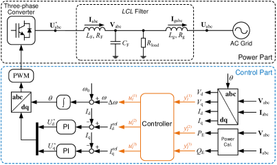
Figure 1: The one-line diagram of a grid-connected power converter [22, Fig. 1].

The AC grid in the power part of Fig. 1 is modeled as an infinite bus with fixed voltage ($1$ p.u.) and fixed frequency ($1$ p.u.). This model has $n=6$ states, $m=3$ inputs and $p=3$ outputs. The inputs are the angular frequency correction $\Delta\omega$ and current references $I^{\rm ref}_{\rm d}$ and $I^{\rm ref}_{\rm q}$ of d- and q-axes, respectively. The outputs to be controlled are the q-axis voltage $V_{\rm q}$, the active power $P_{\rm E}$ and the reactive power $Q_{\rm E}$. The LCL-filter parameters and the PI parameters in Fig. 1 are consistent with [22], whereas the load resistance $R_{\rm load}$ is chosen as a Gaussian signal with mean $4$ p.u. and noise power $10^{-3}$ p.u., which introduces process noise. The measurement noise on each output is normally distributed with variance $10^{-8}$ p.u..

4.1 Benchmark Control Methods

In this subsection, we review several existing receding-horizon control methods which are performed in our simulations and compared to our proposed SDDPC.

4.1.1 Stochastic MPC and (Deterministic) MPC

We investigate two model-based methods, namely Stochastic MPC (SMPC) (Subsection 2.1) and deterministic MPC (or MPC). For both SMPC and MPC, a system model $(A,B,C)$ is obtained through the N4SID system identification method [40], using offline data $u^{\rm d},y^{\rm d}$ collected from the system. MPC follows a similar receding-horizon control process as SMPC, whereas the optimization problem solves for control actions with no feedback policy, and considers deterministic safety constraints

$$E^{\sf u}u_{t}\leq f^{\sf u},\qquad E^{\sf y}y_{t}\leq f^{\sf y}.$$ (42)

The MPC optimization problem at control step $t=k$ is

$$\operatorname*{minimize}_{u,y}\quad \textstyle{\sum_{t=k}^{k+N-1}}J(u_{t},y_{t})$$

$$\mathrm{subject\;to}\quad \eqref{Eq:LTI_deterministic},\eqref{Eq:constraints_deterministic}\text{ for }t\in\mathbb{Z}_{[k,k+N)}\text{, and }x_{k}=\mu^{\sf x}_{k},$$

where the state estimate $\mu^{\sf x}_{k}\leftarrow\hat{x}^{\scalebox{1.2}[1.0]{-}}_{k}$ is obtained by applying Kalman filter (6).

4.1.2 DeePC and SPC

We investigate L2-regularized DeePC [22] and regularized SPC [14] as benchmark data-driven methods. In DeePC and SPC, the optimization problems directly compute control actions while accounting for deterministic safety constraints (42). Using offline data $u^{\rm d},y^{\rm d}$, we formulate data Hankel matrices $U_{\rm p},U_{\rm f},Y_{\rm p},Y_{\rm f}$ similar to $U_{1},U_{2},Y_{1},Y_{2}$ in (23), but matrices $U_{\rm p},U_{\rm f},Y_{\rm p},Y_{\rm f}$ have $mL,mN,pL,pN$ rows respectively. The regularized DeePC optimization problem at control step $t=k$,

$$\begin{aligned} \operatorname*{minimize}_{g,u_{\rm f},y_{\rm f},\sigma_{\rm y}}\quad&\Big{[}\textstyle{\sum_{t=k}^{k+N-1}}J(u_{t},y_{t})\Big{]}+\lambda_{\rm y}\|\sigma_{\rm y}\|^{2}_{2}+\lambda_{\rm g}\|g\|^{2}_{2}\\ \mathrm{subject\;to}\quad&\mathrm{col}(U_{\rm p},Y_{\rm p},U_{\rm f},Y_{\rm f})\;g=\mathrm{col}(u_{\rm ini},y_{\rm ini}\!+\!\sigma_{\rm y},u_{\rm f},y_{\rm f})\\ &\eqref{Eq:constraints_deterministic}\text{ for }t\in\mathbb{Z}_{[k,k+N)}\end{aligned}$$

where $u_{\rm ini}:=u_{[k-L,k)}$, $u_{\rm f}:=u_{[k,k+N)}$ and similarly for $y_{\rm ini}$ and $y_{\rm f}$; $\lambda_{\rm y}>0$ and $\lambda_{\rm g}>0$ are regularization parameters. The SPC optimization problem at control step $t=k$,

$$\operatorname*{minimize}_{u_{\rm f},y_{\rm f}}\quad \textstyle{\sum_{t=k}^{k+N-1}}J(u_{t},y_{t})$$

$$\mathrm{subject\;to}\quad y_{\rm f}=\widehat{\mathcal{P}}_{\sf spc}\;\mathrm{col}(u_{\rm ini},y_{\rm ini},u_{\rm f})$$

$$\eqref{Eq:constraints_deterministic}\text{ for }t\in\mathbb{Z}_{[k,k+N)}$$

where $\widehat{\mathcal{P}}_{\sf spc}$ is the Tikhonov regularization of the prediction matrix $\mathcal{P}_{\sf spc}:=Y_{\rm f}\,\mathrm{col}(U_{\rm p},Y_{\rm p},U_{\rm f})^{\dagger}$, obtained similarly as $\widehat{\mathcal{P}}$ in Subsection 3.1, with a regularization parameter $\lambda>0$.

4.2 Offline Data Collection

Offline data is required in all our investigated control methods, for use in either data matrices (SDDPC, DeePC and SPC) or for system identification (MPC and SMPC). In our simulation, the data collection process lasted for $1$ second and produced a data trajectory of length $T_{\rm d}=1000$ with a sampling period of $1$ms. The input data was generated as follows: $\Delta\omega$ (input 1) was set as the phase-locked loop (PLL) control action (see e.g. [18]) plus a white-noise signal, $I^{\rm ref}_{\rm d}$ (input 2) was set as $0.4$ p.u. plus a white-noise signal, and $I^{\rm ref}_{\rm q}$ (input 3) was set at $0$ p.u. plus a white-noise signal. Each white noise signal had noise power of $10^{-6}$ p.u..

Table 1: Control Parameters

Time Horizon Lengths
Initial-condition horizon length	$L=10$
Prediction horizon length	$N=30$
Control horizon length	$N_{\rm c}=10$
Problem Setup Parameters
Sampling Period	$T_{\rm s}=1$ms
Cost matrices	$Q=10^{4}I_{p}$, $R=I_{m}$
Input constraint coefficients	$E^{\sf u}=I_{m}\otimes\begin{bmatrix}1\\ -1\end{bmatrix}$
	$f^{\sf u}=0.6\times\mathbf{1}_{2m\times 1}$
Output constraint coefficients	$E^{\sf y}=I_{p}\otimes\begin{bmatrix}1\\ -1\end{bmatrix}$
	$f^{\sf y}=0.4\times\mathbf{1}_{2p\times 1}$
Risk probability bounds	$p^{\sf u}=0.2$, $p^{\sf y}=0.2$
Variance of $v_{t}$ for SMPC/SDDPC	$\Sigma^{\sf v}=10^{-8}I_{p}$
Variance of $\rho_{t}$ for SDDPC	$\Sigma^{\rho}=10^{-4}I_{pL}$
Variance of $w_{t}$ for SMPCa	$\Sigma^{\sf w}=\mathcal{O}^{\dagger}\Sigma^{\rho}\mathcal{O}^{\dagger{\sf T}}$
Regularization Parameters
DeePC regularization	$\lambda_{\rm y}=10^{6}$,   $\lambda_{\rm g}=10^{3}$
Regularization of $\mathcal{P}$ in SDDPC	$\lambda=10^{-3}$
Regularization of $\mathcal{P}_{\sf spc}$ in SPC	$\lambda=10^{-3}$
a  In computation of $\Sigma^{\sf w}$, matrix $\mathcal{O}$ is obtained given the
identified system $(A,B,C)$ in SMPC.

4.3 Results

All controller parameters are reported in Table 1. Our simulation consists of two parts. In the first part, we compare the tracking performances of the different controllers. In the second part, we examine the ability of the controllers to maintain safety constraints.

4.3.1 Tracking Performance

For each controller, we perform the following control process. From time $0$s to time $0.2$s, the controller is switched off, and the inputs $I_{\rm d}^{\rm ref}$ and $I_{\rm q}^{\rm ref}$ are set to zero, with $\Delta\omega$ generated from the PLL. After time $0.2$s, the controller is switched on, and the output reference signal is $r_{t}=[0,0,0]^{\sf T}$ before time $0.5$s and $r_{t}=[0,0.3,0]^{\sf T}$ after time $0.5$s. To quantitatively compare the results, Fig. 2 shows the stage cost accumulated over the first two seconds for each controller. The result shows that the stochastic control methods (SMPC and SDDPC) outperformed the deterministic control methods (DeePC, SPC and MPC) in terms of their cumulative costs. This observation aligns with our expectation that stochastic control performs better with stochastic systems, since the stochastic control methods receive feedback at each time step – more frequently than the deterministic control methods which receive feedback only at each control step, i.e., every $N_{\rm c}=10$ time steps. However, this benefit of stochastic control vanishes when we select shorter control horizons. Fig. 3 shows the cumulative stage costs when the control horizon has length $N_{\rm c}=1$, where we no longer observe a performance gap between all stochastic methods and all deterministic methods. SDDPC and SPC outperformed other controllers. Although we showed the results with different $N_{\rm c}$, we emphasize significance of the $N_{\rm c}=10$ setting, which requires less computation since the optimization problems are solved less frequently.

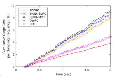
Figure 2: Cumulative stage cost with different controllers, $N_{\rm c}=10$.

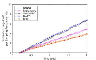
Figure 3: Cumulative stage cost with different controllers, $N_{\rm c}=1$.

4.3.2 Output Constraint Satisfaction

We next evaluate for each controller its ability to meet the output safety constraints. We repeat the control process above, but the reference signal becomes $r_{t}=[0,0,0]^{\sf T}$ before time $0.5$s and $r_{t}=[0,0.5,0]^{\sf T}$ after time $0.5$s. Note that the reference value $0.5$ for the second output channel after time $0.5$s is beyond the range of output safety constraint (with $E^{\sf y},f^{\sf y}$ in TABLE 1), which restricts all output channels within the range of $[-0.4,0.4]$. As a result, in our simulations, the second output channel remained close to the upper safety bound of $0.4$ after time $0.5$s for all controllers; for example, the trace of the second output under SPC and SDDPC is displayed in Fig. 4.

To quantify the constraint satisfaction with each controller, from time $0.5$s to time $2.0$s ($1500$ time steps), we count the number and compute the rate of time steps where the measurement of the second output channel violates the safety constraint. As a second metric, we sum the amount of constraint violation that occurs between $0.5$s to $2.0$s for each controller. The results are displayed in TABLE 2, where we also displayed the results of SMPC and SDDPC with parameter $p^{\sf y}$ changed from $0.2$ (as in TABLE 1) to $0.05$. As the result shows, both violation rates of SMPC and SDDPC declined as we decrease $p^{\sf y}$, while the violation rate of SDDPC shrank more effectively than that of SMPC. The total violation amounts of SMPC and SDDPC also reduced when we decrease $p^{\sf y}$. Among the methods using deterministic safety constraint, DeePC had a lower violation rate and a smaller violation amount than MPC and SPC.

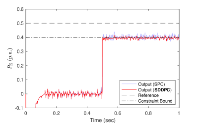
Figure 4: The second output signals with SPC (light blue) and SDDPC (red) in the constraint satisfaction test.

Table 2: Statistics of Constraint Violation
of the Second Output Channel from $0.5$s to $2.0$s

Controller	Violation Rate	Total Violation Amount
SDDPC ($p^{\sf y}=0.2$)	$0.15$	1.10
SDDPC ($p^{\sf y}=0.05$)	$0.03$	0.05
SysID+SMPC ($p^{\sf y}=0.2$)	$0.19$	1.55
SysID+SMPC ($p^{\sf y}=0.05$)	$0.11$	0.52
SysID+MPC	$0.57$	6.79
DeePC	$0.20$	1.46
SPC	$0.49$	8.42

5 Conclusions

We introduced a novel direct data-driven control framework named Stochastic Data-Driven Predictive Control (SDDPC). Analogous to Stochastic MPC (SMPC), SDDPC accounts for process and measurement noise in the control design, and produces closed-loop control policies through optimization. On the theoretical front, we proved that SDDPC can produce control inputs equivalent to those of SMPC under specific conditions. Simulation results indicate that the proposed approach provides benefits in terms of both cumulative stage cost and output constraint violation. Future work will explore recursive feasibility and closed-loops stability of the control scheme, and seek to improve the computational efficiency of the approach. Other important directions include extension to non-Gaussian noise, optimization over the feedback gain $K$, and restriction of violation amount through, e.g., CVaR safety constraints.

[]Ruiqi Li (S’22) received the B.Sc. degree in Honours Physics from the University of Waterloo, ON, Canada in 2019 and the B.Sc. degree in physics from Beijing Institute of Technology, Beijing, China in 2019. He is currently working towards the Ph.D. degree in Electrical and Computer Engineering at the University of Waterloo, ON, Canada. His research interest includes data-driven control, model predictive control and optimization.

[]John W. Simpson-Porco (S’10–M’15–SM’22) received the B.Sc. degree in engineering physics from Queen’s University, Kingston, ON, Canada in 2010, and the Ph.D. degree in mechanical engineering from the University of California at Santa Barbara, Santa Barbara, CA, USA in 2015.

He is currently an Assistant Professor of Electrical and Computer Engineering at the University of Toronto, Toronto, ON, Canada. He was previously an Assistant Professor at the University of Waterloo, Waterloo, ON, Canada and a visiting scientist with the Automatic Control Laboratory at ETH Zürich, Zürich, Switzerland. His research focuses on feedback control theory and applications of control in modernized power grids.

Prof. Simpson-Porco is a recipient of the Automatica Paper Prize, the Center for Control, Dynamical Systems and Computation Best Thesis Award, and the IEEE PES Technical Committee Working Group Recognition Award for Outstanding Technical Report. He is currently an Associate Editor for the IEEE Transactions on Smart Grid.

[]Stephen L. Smith (S’05–M’09–SM’15) received the B.Sc. degree in engineering physics from Queen’s University, Canada, in 2003, the M.A.Sc. degree in electrical and computer engineering from the University of Toronto, Canada, in 2005, and the Ph.D. degree in mechanical engineering from the University of California, Santa Barbara, USA, in 2009.

He is currently a Professor in the Department of Electrical and Computer Engineering at the University of Waterloo, Canada, where he holds a Canada Research Chair in Autonomous Systems. He is also Co-Director of the Waterloo Artificial Intelligence Institute. From 2009 to 2011 he was a Postdoctoral Associate in the Computer Science and Artificial Intelligence Laboratory at MIT. He received the Early Researcher Award from the the Province of Ontario in 2016, the NSERC Discovery Accelerator Supplement Award in 2015, and Outstanding Performance Awards from the University of Waterloo in 2016 and 2019.

He is a licensed Professional Engineer (PEng), an Associate Editor of the IEEE Transactions on Robotics and the IEEE Open Journal of Control Systems. He was previously Associate Editor for the IEEE Transactions on Control of Network Systems (2017 - 2022), and was a General Chair of the 2021 30th IEEE International Conference on Robot and Human Interactive Communication (RO-MAN). His main research interests lie in control and optimization for autonomous systems, with a particular emphasis on robotic motion planning and coordination.

Appendix A Proof of (13)

Proof.

We first show for $t\in\mathbb{Z}_{[k,k+N)}$ that

$$\begin{bmatrix}\hat{x}_{t}\\ x_{t}\end{bmatrix}\;\sim\;\mathcal{N}\left(\begin{bmatrix}x_{t}^{\sf nom}\\ x_{t}^{\sf nom}\end{bmatrix},\Sigma^{\sf\hat{x}x}_{t}\right),$$ (43)

with $\Sigma^{\sf\hat{x}x}_{t}$ defined in (15). We prove this by induction on time $t$. Base case $t=k$. Observing that

$$\text{via \eqref{Eq:state_estimation:postetior},}\quad\hat{x}_{k}=(I_{n}-L_{k}C)\hat{x}^{\scalebox{1.2}[1.0]{-}}_{k}+L_{k}y_{k}$$

$$\text{via \eqref{Eq:state_estimation:initial},}\quad\hat{x}^{\scalebox{1.2}[1.0]{-}}_{k}=\mu^{\sf x}_{k}$$

$$\text{via \eqref{Eq:LTI:output},}\quad y_{k}=Cx_{k}+v_{k}$$

we can express $x_{k},\hat{x}_{k}$ in terms of $x_{k},v_{k},\mu^{\sf x}_{k}$ by eliminating $y_{k},\hat{x}^{\scalebox{1.2}[1.0]{-}}_{k}$, yielding

$$\small\begin{bmatrix}\hat{x}_{k}\\ x_{k}\end{bmatrix}=\begin{bmatrix}L_{k}C\\ I_{n}\end{bmatrix}x_{k}+\begin{bmatrix}L_{k}\\ 0\end{bmatrix}v_{k}+\begin{bmatrix}(I_{n}-L_{k}C)\mu^{\sf x}_{k}\\ 0\end{bmatrix},$$ (44)

where we know that $x_{k}\sim\mathcal{N}(\mu^{\sf x}_{k},\Sigma^{\sf x}_{k})$ via (5) and $v_{k}\sim\mathcal{N}(0,\Sigma^{\sf v})$ via (2). Note that $x_{k}$ and $v_{k}$ are independent because $x_{k}$ via (1a) is only decided by $x_{0}$, $u_{[0,k)}$, $w_{[0,k)}$ which are all independent of $v_{k}$. Given (44) and the distribution of $x_{k},v_{k}$, one can compute that the mean of $\mathrm{col}(\hat{x}_{k},x_{k})$ is

$$\small\begin{bmatrix}L_{k}C\\ I_{n}\end{bmatrix}\mu^{\sf x}_{k}+\begin{bmatrix}L_{k}\\ 0\end{bmatrix}0+\begin{bmatrix}(I_{n}-L_{k}C)\mu^{\sf x}_{k}\\ 0\end{bmatrix}=\begin{bmatrix}\mu^{\sf x}_{k}\\[1.79997pt] \mu^{\sf x}_{k}\end{bmatrix}=\begin{bmatrix}x^{\sf nom}_{k}\\[1.79997pt] x^{\sf nom}_{k}\end{bmatrix},$$

where the first equality is direct calculation and the second equality is via (9c). Similarly, the variance of $\mathrm{col}(\hat{x}_{k},x_{k})$ can now be computed as

$$\small\begin{bmatrix}L_{k}C\\ I_{n}\end{bmatrix}\Sigma^{\sf x}_{k}\begin{bmatrix}L_{k}C\\ I_{n}\end{bmatrix}^{\sf T}+\begin{bmatrix}L_{k}\\ 0\end{bmatrix}\Sigma^{\sf v}\begin{bmatrix}L_{k}\\ 0\end{bmatrix}^{\sf T},$$

which is equal to $\begin{bmatrix}L_{k}(C\Sigma^{\sf x}_{k}C^{\sf T}+\Sigma^{\sf v})L_{k}^{\sf T}&L_{k}C\Sigma^{\sf x}_{k}\\ \Sigma^{\sf x}_{k}C^{\sf T}L_{k}^{\sf T}&\Sigma^{\sf x}_{k}\end{bmatrix}$ by matrix multiplication and can be verified equal to matrix $\Sigma^{\sf\hat{x}x}_{k}$ in (15b), given relations $L_{k}(C\Sigma^{\sf x}_{k}C^{\sf T}+\Sigma^{\sf v})=\Sigma^{\sf x}_{k}C^{\sf T}$ via (7a), (7d) and $L_{k}C\Sigma^{\sf x}_{k}=\Sigma^{\sf x}_{k}-P_{k}$ via (7b), (7d). Thus, the base case $t=k$ of (43) is covered. Inductive step. Assume (43) holds for $t=\tau\in\mathbb{Z}_{[k,k+N-2]}$. Using the following relations,

via (6a), $$\hat{x}_{\tau+1} =(I_{n}-L_{\tau+1}C)\hat{x}^{\scalebox{1.2}[1.0]{-}}_{\tau+1}+L_{\tau+1}y_{\tau+1}$$

via (6b), $$\hat{x}^{\scalebox{1.2}[1.0]{-}}_{\tau+1} =A\hat{x}_{\tau}+Bu_{\tau}$$

via (1b), $$y_{\tau+1} =Cx_{\tau+1}+v_{\tau+1}$$

via (1a), $$x_{\tau+1} =Ax_{\tau}+Bu_{\tau}+w_{\tau}$$

via (8), $$u_{\tau} =u^{\sf nom}_{\tau}+K(\hat{x}_{\tau}-x^{\sf nom}_{\tau})$$

we can express $\hat{x}_{\tau+1},x_{\tau+1}$ in terms of $\hat{x}_{\tau}$, $x_{\tau}$, $w_{\tau}$, $v_{\tau+1}$, $x^{\sf nom}_{\tau}$, $u^{\sf nom}_{\tau}$ by eliminating $\hat{x}^{\scalebox{1.2}[1.0]{-}}_{\tau+1},u_{\tau},y_{\tau+1}$,

$$\small\begin{aligned} \begin{bmatrix}\hat{x}_{\tau+1}\\ x_{\tau+1}\end{bmatrix}&=\Lambda_{\tau+1}\begin{bmatrix}\hat{x}_{\tau}\\ x_{\tau}\end{bmatrix}+\underbrace{\begin{bmatrix}L_{\tau+1}C\\ I_{n}\end{bmatrix}w_{\tau}+\begin{bmatrix}L_{\tau+1}\\ 0\end{bmatrix}v_{\tau+1}}_{=:\delta_{\tau+1}}\\ &\quad+\underbrace{\begin{bmatrix}B(u^{\sf nom}_{\tau}-Kx^{\sf nom}_{\tau})\\[1.79997pt] B(u^{\sf nom}_{\tau}-Kx^{\sf nom}_{\tau})\end{bmatrix}}_{=:\gamma_{\tau}}\end{aligned}$$ (45)

where we know $\mathrm{col}(\hat{x}_{\tau},x_{\tau})\sim\mathcal{N}\big{(}\mathrm{col}(x^{\sf nom}_{\tau},x^{\sf nom}_{\tau}),\Sigma^{\sf\hat{x}x}_{\tau}\big{)}$ from the inductive assumption, $\gamma_{\tau}$ is deterministic, and one can check $\delta_{\tau+1}\sim\mathcal{N}(0,\Delta_{\tau+1})$ by direct calculation, with $\Lambda_{\tau+1}$ defined in (16a) and $\Delta_{\tau+1}$ defined in (16b). Note that $\mathrm{col}(\hat{x}_{\tau},x_{\tau})$ and $\delta_{\tau+1}$ are independent, given the definition of $\delta_{\tau+1}$ and the fact that both $\hat{x}_{\tau}$ and $x_{\tau}$ are independent of $w_{\tau},v_{\tau+1}$. Hence, given (45) and the distributions of $\mathrm{col}(\hat{x}_{\tau},x_{\tau})$ and $\delta_{\tau+1}$, the mean of $\mathrm{col}(\hat{x}_{\tau+1},x_{\tau+1})$ is what follows,

$$\Lambda_{\tau+1}\begin{bmatrix}x^{\sf nom}_{\tau}\\ x^{\sf nom}_{\tau}\end{bmatrix}+\gamma_{\tau}=\begin{bmatrix}Ax^{\sf nom}_{\tau}+Bu^{\sf nom}_{\tau}\\ Ax^{\sf nom}_{\tau}+Bu^{\sf nom}_{\tau}\end{bmatrix}=\begin{bmatrix}x^{\sf nom}_{\tau+1}\\ x^{\sf nom}_{\tau+1}\end{bmatrix}$$

where the first equality above is direct substitution of $\Lambda_{\tau+1}$ and $\gamma_{\tau}$, and the second equality is via (9a). Similarly from (45), the variance of $\mathrm{col}(\hat{x}_{\tau+1},x_{\tau+1})$ is

$$\Lambda_{\tau+1}\Sigma^{\sf\hat{x}x}_{\tau}\Lambda_{\tau+1}^{\sf T}+\Delta_{\tau+1},$$

which equals the definition of $\Sigma^{\sf\hat{x}x}_{\tau+1}$ in (15a). This shows the $t=\tau+1$ case of (43). By induction on $t$, (43) holds for all $t\in\mathbb{Z}_{[k,k+N)}$.

Finally, we prove (13) with $\Sigma^{\sf u}_{t},\Sigma^{\sf y}_{t}$ in (14). Rewrite (1b) and (8) as follows,

$$\begin{aligned} &u_{t}\overset{\text{via \eqref{Eq:feedback_policy}}}{=}\big{[}K,0_{m\times n}\big{]}\,\mathrm{col}(\hat{x}_{t},x_{t})+(u^{\sf nom}_{t}-Kx^{\sf nom}_{t})\\ &y_{t}\overset{\text{via \eqref{Eq:LTI:output}}}{=}\big{[}0_{p\times n},C\big{]}\,\mathrm{col}(\hat{x}_{t},x_{t})+v_{t}\end{aligned}$$ (46)

where we have $\mathrm{col}(\hat{x}_{t},x_{t})\sim\mathcal{N}(\mathrm{col}(x^{\sf nom}_{t},x^{\sf nom}_{t}),\Sigma^{\sf\hat{x}x}_{k})$ via (43) and $v_{t}\sim\mathcal{N}(0,\Sigma^{\sf v})$ via (2). Also, $\mathrm{col}(\hat{x}_{t},x_{t})$ is independent of $v_{t}$. With (46) and the distributions of $\mathrm{col}(\hat{x}_{t},x_{t})$ and $v_{t}$, one can calculate that the means of $u_{t}$ and $y_{t}$ are $u^{\sf nom}_{t}$ and $Cx^{\sf nom}_{t}\overset{\text{via \eqref{Eq:nominal_state:output}}}{=}y^{\sf nom}_{t}$ respectively, and the variances of $u_{t}$ and $y_{t}$ are $\Sigma^{\sf u}_{t}$ and $\Sigma^{\sf y}_{t}$ given in (14) respectively. This indicates that (13) is correct. ∎

Appendix B Iterative Risk Allocation

We record here an efficient method for solving the convex problem (20), known as Iterative Risk Allocation [38], described in Algorithm 3.

To begin, note that if we fix all variables $p^{\sf u}_{i,t}$ and $p^{\sf y}_{i,t}$, then problem (20) is reduced into the quadratic problem

$$\begin{aligned} \operatorname*{minimize}_{u^{\sf nom}}\quad&\textstyle{\sum_{t=k}^{k+N-1}}J(u^{\sf nom}_{t},y^{\sf nom}_{t})\\ \mathrm{subject\;to}\quad&\text{\eqref{Eq:constraints_reduced:input_constraints}, \eqref{Eq:constraints_reduced:output_constraints} for all $t\in\mathbb{Z}_{[k,k+N)}$, and \eqref{Eq:nominal_state}}\end{aligned}$$ (47)

Algorithm 3 Iterative Risk Allocation for solving (20)

1:horizon length $N$, system matrices $A,B,C$, state mean $\mu^{\sf x}_{k}$, cost matrices $Q$, $R$, constraint coefficients $E^{\sf u}$, $E^{\sf y}$, $f^{\sf u}$, $f^{\sf y}$, probability bounds $p^{\sf u}$, $p^{\sf y}$, input-output variances $\Sigma^{\sf u}_{[k,k+N)}$, $\Sigma^{\sf y}_{[k,k+N)}$, shrinkage rate $\alpha$, termination threshold $\varepsilon$.

2:An approximate solution to (20), including the nominal input $u^{\sf nom}_{[k,k+N)}$ and output $y^{\sf nom}_{[k,k+N)}$ and the allocated probabilities $\{p^{\sf u}_{i,t}\}_{i=1}^{q^{\sf u}}$, $\{p^{\sf y}_{i,t}\}_{i=1}^{q^{\sf y}}$ for $t\in\mathbb{Z}_{[k,k+N)}$.

3:Initialize $p^{\sf u}_{i,t}\leftarrow p^{\sf u}/q^{\sf u}$ for all $i\in\{1,\ldots,q^{\sf u}\}$ and all $t\in\mathbb{Z}_{[k,k+N)}$.

4:Initialize $p^{\sf y}_{i,t}\leftarrow p^{\sf y}/q^{\sf y}$ for all $i\in\{1,\ldots,q^{\sf y}\}$ and all $t\in\mathbb{Z}_{[k,k+N)}$.

5:Initialize $J^{\star}_{\sf prev}\leftarrow+\infty$.

6:while true do

7:      Solve $u^{\sf nom}$, $y^{\sf nom}$ from problem (47) and obtain the cost value $J^{\star}$. Record whether the constraints (19a), (19b) are active or not for each $(i,t)$.

8:     if $|J^{\star}_{\sf prev}-J^{\star}|\leq\varepsilon$ then break else $J^{\star}_{\sf prev}\leftarrow J^{\star}$.

9:      For $t\in\mathbb{Z}_{[k,k+N)}$ and $i\in\{1,\ldots,q^{\sf u}\}$, let $a^{\sf u}_{i,t}\leftarrow 1$ if constraint (19a) is active for $(i,t)$, otherwise $a^{\sf u}_{i,t}\leftarrow 0$.

10:      For $t\in\mathbb{Z}_{[k,k+N)}$ and $i\in\{1,\ldots,q^{\sf y}\}$, let $a^{\sf y}_{i,t}\leftarrow 1$ if constraint (19b) is active for $(i,t)$, otherwise $a^{\sf y}_{i,t}\leftarrow 0$.

11:      $a^{\sf u,sum}_{t}\leftarrow\sum_{i=1}^{q^{\sf u}}a^{\sf u}_{i,t}$ and $a^{\sf y,sum}_{t}\leftarrow\sum_{i=1}^{q^{\sf y}}a^{\sf y}_{i,t}$ for all $t\in\mathbb{Z}_{[k,k+N)}$.

12:      if $a^{\sf u,sum}_{t}\in\{0,q^{\sf u}\}$ and $a^{\sf y,sum}_{t}\in\{0,q^{\sf y}\}$ for all $t\in\mathbb{Z}_{[k,k+N)}$ then break.

13:      $\{p^{\sf u}_{i,t}\}\leftarrow$ Update($\{p^{\sf u}_{i,t}\}$, $\{a^{\sf u}_{i,t}\}$, $u^{\sf nom}$, $\{\Sigma^{\sf u}_{t}\}$, $p^{\sf u}$, $q^{\sf u}$, $E^{\sf u}$, $f^{\sf u}$, $\alpha$)

14:      $\{p^{\sf y}_{i,t}\}\leftarrow$ Update($\{p^{\sf y}_{i,t}\}$, $\{a^{\sf y}_{i,t}\}$, $y^{\sf nom}$, $\{\Sigma^{\sf y}_{t}\}$, $p^{\sf y}$, $q^{\sf y}$, $E^{\sf y}$, $f^{\sf y}$, $\alpha$)

which can be efficiently solved. The optimal solution to (20) is the infimum of the solution to (47) over all $p^{\sf u}_{i,t}$ and $p^{\sf y}_{i,t}$ satisfying (19c) and (19d). Hence, we solve problem (47) repeatedly with updated $p^{\sf u}_{i,t}$ and $p^{\sf y}_{i,t}$, until the objective value converges with no significant change. The entire process shows in Algorithm 3, which extends [38, Algorithm 1] from their single-joint-chance-constraint case into our multiple-separate-chance-constraint case. Newly introduced parameters are the shrinkage rate $\alpha\in(0,1)$ and the termination threshold $\varepsilon>0$. From lines 9-10, we obtain indicators $a^{\sf u}_{i,t}$ and $a^{\sf y}_{i,t}$ showing whether constraints (19a) and (19b) are active or not for each $(i,t)$. Those indicators are utilized in the process of updating $p^{\sf u}_{i,t}$ and $p^{\sf y}_{i,t}$ in lines 13-14, where we use a subroutine Update shown in Algorithm 4. Note that, when the condition in line 12 is true, the subroutine Update no longer makes change on $p^{\sf u}_{i,t}$ and $p^{\sf y}_{i,t}$, so in this case the iteration terminates. In line 6 of Algorithm 4, $\mathrm{cdfn}(z):=\frac{1}{2}+\frac{1}{2}\mathrm{erf}(z/\sqrt{2})$ is the c.d.f. of the standard normal distribution, with $\mathrm{erf}$ the error function.

Similarly, problem (38) can also be solved by Algorithm 3 with $A$, $B$, $C$, $\mu^{\sf x}_{k}$, $\Sigma^{\sf u}_{t}$, $\Sigma^{\sf y}_{t}$, $y^{\sf nom}_{t}$ replaced by $\mathbf{A}$, $\mathbf{B}$, $\mathbf{C}$, $\boldsymbol{\mu}^{\sf x}_{k}$, $\mathbf{\Sigma}^{\sf u}_{t}$, $\mathbf{\Sigma}^{\sf y}_{t}$, $\mathbf{y}^{\sf nom}_{t}$ respectively.

Algorithm 4 Subroutine Update in Algorithm 3

1:$p^{\sf z}_{i,t}$ and $a^{\sf z}_{i,t}$ for $i\in\{1,\ldots,q^{\sf z}\}$ and $t\in\mathbb{Z}_{[k,k+N)}$, $z^{\sf nom}_{[k,k+N)}$, $\Sigma^{\sf z}_{[k,k+N)}$, $p^{\sf z}$, $q^{\sf z}$, $E^{\sf z}=\mathrm{col}(e^{\sf z{\sf T}}_{1},e^{\sf z{\sf T}}_{2},\ldots,e^{\sf z{\sf T}}_{q^{\sf z}})$, $f^{\sf z}=\mathrm{col}(f^{\sf z}_{1},f^{\sf z}_{2},\ldots,f^{\sf z}_{q^{\sf z}})$ and $\alpha$

2:updated values of $p^{\sf z}_{i,t}$ for $i\in\{1,\ldots,q^{\sf z}\}$ and $t\in\mathbb{Z}_{[k,k+N)}$

3:$a^{\sf z,sum}_{t}\leftarrow\sum_{i=1}^{q^{\sf z}}a^{\sf z}_{i,t}$ for all $t\in\mathbb{Z}_{[k,k+N)}$.

4:for $t\in\mathbb{Z}_{[k,k+N)}$ such that $0<a^{\sf z,sum}_{t}<q^{\sf z}$ do

5:     for all $i\in\{1,\ldots,q^{\sf z}\}$ such that $a^{\sf z}_{i,t}=0$ do

6:         $p^{\sf z}_{i,t}\leftarrow\alpha p^{\sf z}_{i,t}+(1-\alpha)\bigg{(}1-\mathrm{cdfn}\bigg{(}\displaystyle{\frac{f^{\sf z}_{i}-e^{\sf z{\sf T}}_{i}z^{\sf nom}_{t}}{\sqrt{e^{\sf z{\sf T}}_{i}\Sigma^{\sf z}_{t}e^{\sf z}_{i}}}}\bigg{)}\bigg{)}$.      

7:     $p^{\sf z,residual}_{t}\leftarrow p^{\sf z}-\sum_{i=1}^{q^{\sf z}}p^{\sf z}_{i,t}$.

8:     for all $i\in\{1,\ldots,q^{\sf z}\}$ such that $a^{\sf z}_{i,t}=1$ do

9:         $p^{\sf z}_{i,t}\leftarrow p^{\sf z}_{i,t}+p^{\sf z,residual}_{t}/a^{\sf z,sum}_{t}$.      

Appendix C Proof of Lemma 3

Proof.

Let $(x^{\rm d},u^{\rm d},y^{{\rm d}})$ be the state-input-output trajectory of (22), and define $X_{1},X_{2}\in{}^{n\times h}$ as

$$X_{1}:=\big{[}x^{\rm d}_{1},x^{\rm d}_{2},\ldots,x^{\rm d}_{h}\big{]},\;\;X_{2}:=\big{[}x^{\rm d}_{1+L},x^{\rm d}_{2+L},\ldots,x^{\rm d}_{h+L}\big{]}.$$

It follows by straightforward algebra that data matrices satisfy [14, eq. 3.20-3.22]

$$X_{2} =A^{L}X_{1}+\mathcal{C}U_{1}$$ (48a)

$$Y_{1} =\mathcal{O}X_{1}+\mathbf{G}U_{1}$$ (48b)

$$Y_{2} =\mathcal{O}X_{2}+\mathbf{G}U_{2}.$$ (48c)

Under our assumptions of controllability and persistency of excitation, it follows from [41, Corollary 2(iii)] that the matrix $\mathrm{col}(X_{1},U_{1},U_{2})$ has full row rank. Moreover, $\begin{bmatrix}I_{mL}\\ \mathbf{G}&\mathcal{O}\end{bmatrix}$ and $\begin{bmatrix}I_{mL}\\ \mathbf{G}&\mathcal{O}\\ &&I_{mL}\end{bmatrix}$ have full column rank, as they are block lower triangular and their diagonal blocks each has full column rank (Section 3.1).

First we show that $[\mathcal{P}_{1},\mathcal{P}_{2},\mathcal{P}_{3}]=[\mathbf{\Gamma}_{\sf U},\mathbf{\Gamma}_{\sf Y},\mathbf{G}]$. Recall that $[\mathcal{P}_{1},\mathcal{P}_{2},\mathcal{P}_{3}]$ is defined as $Y_{2}\,\mathrm{col}(U_{1},Y_{1},U_{2})^{\dagger}$. First, the matrix $Y_{2}$ can be represented in terms of $X_{1},U_{1},U_{2}$ by combining (48a) and (48c) and eliminating $X_{2}$,

$$Y_{2}=\big{[}\underbrace{\mathcal{O}\mathcal{C}}_{=\mathbf{H}}\,,\,\mathcal{O}A^{L}\,,\,\mathbf{G}\big{]}\footnotesize\begin{bmatrix}U_{1}\\ X_{1}\\ U_{2}\end{bmatrix},$$ (49)

where we have $\mathbf{H}=\mathcal{O}\mathcal{C}$ in (49) according to the definition of $\mathbf{H},\mathcal{O},\mathcal{C}$. We can also represent $\mathrm{col}(U_{1},Y_{1},U_{2})$ in terms of $X_{1},U_{1},U_{2}$ using (48b) as

$$\footnotesize\begin{bmatrix}U_{1}\\ Y_{1}\\ U_{2}\end{bmatrix}=\begin{bmatrix}I_{mL}&&\\ \mathbf{G}&\mathcal{O}&\\ &&I_{mL}\end{bmatrix}\begin{bmatrix}U_{1}\\ X_{1}\\ U_{2}\end{bmatrix}.$$

As we know that $\begin{bmatrix}I_{mL}&&\\ \mathbf{G}&\mathcal{O}&\\ &&I_{mL}\end{bmatrix}$ has full column rank and $\begin{bmatrix}U_{1}\\ X_{1}\\ U_{2}\end{bmatrix}$ has full row rank, the pseudo-inverse of above is [42]

$$\footnotesize\begin{bmatrix}U_{1}\\ Y_{1}\\ U_{2}\end{bmatrix}^{\dagger}=\begin{bmatrix}U_{1}\\ X_{1}\\ U_{2}\end{bmatrix}^{\dagger}\begin{bmatrix}I_{mL}&&\\ \mathbf{G}&\mathcal{O}&\\ &&I_{mL}\end{bmatrix}^{\dagger}.$$ (50)

Thus, by multiplying (49) and (50), we find that

$$\begin{aligned} \footnotesize[\mathcal{P}_{1},\mathcal{P}_{2},\mathcal{P}_{3}]&=Y_{2}\,\mathrm{col}(U_{1},Y_{1},U_{2})^{\dagger}\\ &=\big{[}\mathbf{H},\mathcal{O}A^{L},\mathbf{G}\big{]}\footnotesize\begin{bmatrix}I_{mL}\\ \mathbf{G}&\mathcal{O}\\ &&I_{mL}\end{bmatrix}^{\dagger}\\ &=\begin{bmatrix}\big{[}\mathbf{H},\mathcal{O}A^{L}\big{]}\footnotesize\begin{bmatrix}I_{mL}\\ \mathbf{G}&\mathcal{O}\end{bmatrix}^{\dagger}&\mathbf{G}\end{bmatrix}\\ &\!\!\!\!\!\overset{\text{via \eqref{Eq:GammaMatrix:entire}}}{=}[\mathbf{\Gamma}_{\sf U},\mathbf{\Gamma}_{\sf Y},\mathbf{G}].\end{aligned}$$ (51)

Finally, given (25a) with $\begin{bmatrix}I_{mL}\\ \mathbf{G}&\mathcal{O}\end{bmatrix}$ of full column rank, we have

$$\footnotesize[\mathbf{H},\mathcal{O}A^{L}] =[\mathbf{\Gamma}_{\sf U},\mathbf{\Gamma}_{\sf Y}]\footnotesize\begin{bmatrix}I_{mL}\\ \mathbf{G}&\mathcal{O}\end{bmatrix}$$ (52)

$$=[\mathbf{\Gamma}_{\sf U}+\mathbf{\Gamma}_{\sf Y}\mathbf{G},\;\mathbf{\Gamma}_{\sf Y}\mathcal{O}]$$

$$\!\!\!\!\overset{\text{via \eqref{Eq:PROOF:data_representation:result_1}}}{=}[\mathcal{P}_{1}+\mathcal{P}_{2}\mathcal{P}_{3},\;\mathbf{\Gamma}_{\sf Y}\mathcal{O}],$$

which shows that $\mathbf{H}=\mathcal{P}_{1}+\mathcal{P}_{2}\mathcal{P}_{3}$ and completes the proof. ∎

Appendix D Proof of Lemma 4

Proof.

We first show that we can construct a matrix $\Phi\in{}^{n\times n_{\sf aux}}$ such that $x_{t}=\Phi\mathbf{x}_{t}$. Given the system model (1), the state $x_{t}$ and noise-free output $y^{\circ}_{[t-L,t)}$ can be expressed in terms of a previous state $x_{t-L}$, previous inputs $u_{[t-L,t)}$ and previous disturbances $w_{[t-L,t)}$ via

$$x_{t} =A^{L}\,x_{t-L}+\mathcal{C}\,u_{[t-L,t)}+\mathcal{C}_{\sf W}\,w_{[t-L,t)}$$ (53a)

$$y^{\circ}_{[t-L,t)} =\mathcal{O}\,x_{t-L}+\mathbf{G}\,u_{[t-L,t)}+\mathbf{G}_{\sf W}\,w_{[t-L,t)},$$ (53b)

where $\mathcal{C}_{\sf W}:=[A^{L-1},\ldots,A,I_{n}]\in{}^{n\times nL}$, and $\mathbf{G}_{\sf W}\in{}^{pL\times nL}$ is defined as

$$\mathbf{G}_{\sf W}:=\footnotesize\begin{bmatrix}0_{p\times n}\\ C&0_{p\times n}\\[-4.0pt] \vdots&\ddots&\ddots\\ CA^{L-2}&\cdots&C&0_{p\times n}\end{bmatrix}.$$

Define $[\Phi_{\sf U},\Phi_{\sf Y}]:=[\mathcal{C},A^{L}]\begin{bmatrix}I_{mL}\\ \mathbf{G}&\mathcal{O}\end{bmatrix}^{\dagger}\in{}^{n\times(m+p)L}$. Since $\mathcal{O}$ has full column rank, so does $\begin{bmatrix}I_{mL}\\ \mathbf{G}&\mathcal{O}\end{bmatrix}$, and therefore

$$\begin{aligned} =[\Phi_{\sf U},\Phi_{\sf Y}]\small\begin{bmatrix}I_{mL}\\ \mathbf{G}&\mathcal{O}\end{bmatrix}=[\Phi_{\sf U}+\Phi_{\sf Y}\mathbf{G},\Phi_{\sf Y}\mathcal{O}].\end{aligned}$$ (54)

Left-multiply (53b) by $\Phi_{\sf Y}$, and we have

$$\begin{aligned} &\quad\Phi_{\sf Y}(-\mathbf{G}u_{[t-L,t)}+y^{\circ}_{[t-L,t)}-\mathbf{G}_{\sf W}w_{[t-L,t)})\\ &=\Phi_{\sf Y}\mathcal{O}x_{t-L}\overset{\text{via \eqref{Eq:PROOF:DDModel:Phi_relation}}}{=}A^{L}x_{t-L}.\end{aligned}$$ (55)

Substituting (55) into (53a), we eliminate $A^{L}x_{t-L}$ and express $x_{t}$ in terms of $u$, $y^{\circ}$ and $w$ as

$$x_{t} =\underbrace{(\mathcal{C}-\Phi_{\sf Y}\mathbf{G})}_{=\Phi_{\sf U}\text{ via \eqref{Eq:PROOF:DDModel:Phi_relation}}}u_{[t-L,t)}+\Phi_{\sf Y}\,y^{\circ}_{[t-L,t)}$$

$$\quad+\underbrace{(\mathcal{C}_{\sf W}-\Phi_{\sf Y}\mathbf{G}_{\sf W})}_{=:\,\Phi_{\sf W}}w_{[t-L,t)}.$$

Define $\Phi_{\rho}:=\Phi_{\sf W}\,(I_{L}\otimes\mathcal{O}^{\dagger})$. Then, we write the last term above as $\Phi_{\sf W}\,w_{[t-L,t)}=\Phi_{\sf W}\,(I_{L}\otimes\mathcal{O}^{\dagger})\,\rho_{[t-L,t)}=\Phi_{\rho}\,\rho_{[t-L,t)}$, where the first equality used the fact $w_{[t-L,t)}=(I_{L}\otimes\mathcal{O}^{\dagger})\,\rho_{[t-L,t)}$ given the definition $\rho_{t}:=\mathcal{O}w_{t}$ with $\mathcal{O}$ of full column rank. Hence, the above equation can be written as $x_{t}=\Phi\,\mathbf{x}_{t}$ with $\Phi:=[\Phi_{\sf U},\Phi_{\sf Y},\Phi_{\rho}]$, given the definition of $\mathbf{x}_{t}$ in (26).

Next, we show the relation (27b). Given (25b), the definition of $\Phi_{\sf U},\Phi_{\sf Y}$ and the fact that $C\mathcal{C}=\mathbf{H_{1}}$ (which can be verified given the definition of $\mathcal{C}$ and $\mathbf{H_{1}}$), we know that

$$C[\Phi_{\sf U},\Phi_{\sf Y}]=[\mathbf{\Gamma}_{\sf U\bf 1},\mathbf{\Gamma}_{\sf Y\bf 1}].$$ (56)

Given the definition $\Phi_{\sf W}:=\mathcal{C}_{\sf W}-\Phi_{\sf Y}\mathbf{G}_{\sf W}$, we have

$$\begin{aligned} C\Phi_{\sf W}&=C\mathcal{C}_{\sf W}-C\Phi_{\sf Y}\mathbf{G}_{\sf W}\overset{\text{via \eqref{Eq:PROOF:DDModel:c_relation_uy}}}{=}C\mathcal{C}_{\sf W}-\mathbf{\Gamma}_{\sf Y\bf 1}\mathbf{G}_{\sf W}\\ &=\mathbf{F}(I_{L}\otimes\mathcal{O})-\mathbf{\Gamma}_{\sf Y\bf 1}\mathbf{E}(I_{L}\otimes\mathcal{O})\end{aligned}$$ (57)

where the last equality used the facts that $C\mathcal{C}_{\sf W}=\mathbf{F}(I_{L}\otimes\mathcal{O})$ and $\mathbf{G}_{\sf W}=\mathbf{E}(I_{L}\otimes\mathcal{O})$ which both can be verified from the definition of $\mathbf{E},\mathbf{F},\mathcal{C}_{\sf W},\mathbf{G}_{\sf W}$. Given the definition $\Phi_{\rho}:=\Phi_{\sf W}(I_{L}\otimes\mathcal{O}^{\dagger})$, it follows from (57) that

$$C\Phi_{\rho}=(\mathbf{F}-\mathbf{\Gamma}_{\sf Y\bf 1}\mathbf{E})(I_{L}\otimes\mathcal{O}\mathcal{O}^{\dagger}).$$ (58)

Recall $\mathbf{C}:=[\mathbf{\Gamma}_{\sf U\bf 1},\mathbf{\Gamma}_{\sf Y\bf 1},\mathbf{F}-\mathbf{\Gamma}_{\sf Y\bf 1}\mathbf{E}]$ and $\Phi:=[\Phi_{\sf U},\Phi_{\sf Y},\Phi_{\rho}]$, so the horizontal stack of (56) and (58) can be written as

$$C\,\Phi=\mathbf{C}\underbrace{\begin{bmatrix}I_{mL}\\ &I_{pL}\\ &&I_{L}\otimes\mathcal{O}\mathcal{O}^{\dagger}\end{bmatrix}}_{=:\,J}.$$ (59)

Notice that $J\mathbf{x}_{t}=\mathbf{x}_{t}$ because $(I_{L}\otimes\mathcal{O}\mathcal{O}^{\dagger})\rho_{[t-L,t)}=\rho_{[t-L,t)}$, which follows from the fact that $\mathcal{O}\mathcal{O}^{\dagger}\rho_{t}=\mathcal{O}\mathcal{O}^{\dagger}\mathcal{O}w_{t}=\mathcal{O}w_{t}=\rho_{t}$. Thus, we obtain (27b).

$$y_{t} \overset{\text{via \eqref{Eq:LTI:output}}}{=}Cx_{t}+v_{t}=C\Phi\mathbf{x}_{t}+v_{t}\overset{\text{via \eqref{Eq:PROOF:DDModel:c_relation}}}{=}\mathbf{C}J\mathbf{x}_{t}+v_{t}$$

$$\;\;\;=\mathbf{C}\mathbf{x}_{t}+v_{t}$$

Last, we prove (27a). Using the definitions of $\mathbf{x}_{t},\mathbf{w}_{t}$ in (26) and the definitions of $\mathbf{A},\mathbf{B}$, by direct matrix multiplication, we have the following.

$$\small\begin{aligned} \mathbf{A}\mathbf{x}_{t}&=\left[\begin{array}[]{c}u_{[t-L+1,t)}\\ 0_{m\times 1}\\ \hline\cr y^{\circ}_{[t-L+1,t)}\\ \mathbf{C}\mathbf{x}_{t}\\ \hline\cr\rho_{[t-L+1,t)}\\ 0_{pL\times 1}\end{array}\right]\overset{\text{via \eqref{Eq:DDModel:output}}}{=}\left[\begin{array}[]{c}u_{[t-L+1,t)}\\ 0_{m\times 1}\\ \hline\cr y^{\circ}_{[t-L+1,t)}\\ y^{\circ}_{t}\\ \hline\cr\rho_{[t-L+1,t)}\\ 0_{pL\times 1}\end{array}\right],\\ \mathbf{B}u_{t}&=\left[\begin{array}[]{c}0_{m(L-1)\times 1}\\ u_{t}\\ \hline\cr 0_{pL\times 1}\\ \hline\cr 0_{pL^{2}\times 1}\end{array}\right],\quad\mathbf{w}_{t}=\left[\begin{array}[]{c}0_{mL\times 1}\\ \hline\cr 0_{pL\times 1}\\ \hline\cr 0_{pL(L-1)\times 1}\\ \rho_{t}\end{array}\right].\end{aligned}$$

Adding the above equalities together, the left-hand side yields $\mathbf{A}\mathbf{x}_{t}+\mathbf{B}u_{t}+\mathbf{w}_{t}$, and the right-hand side is $\mathbf{x}_{t+1}$ by definition, so (27a) is obtained. ∎

Appendix E Proof of Lemma 5

Proof.

The pair $(\mathbf{A},\mathbf{C})$ is detectable by definition since there exists a matrix $\mathbf{L}^{\prime}:=\mathrm{col}(0_{mL\times p},0_{p(L-1)\times p},I_{p},0_{pL^{2}\times p})$ such that $\mathbf{A}-\mathbf{L}^{\prime}\mathbf{C}$ equal to

$$\left[\footnotesize\begin{array}[]{c|c|c}\begin{matrix}&I_{m(L-1)}\\ 0_{m\times m}\end{matrix}&0&0\\ \hline\cr 0&\begin{matrix}&I_{p(L-1)}\\ 0_{p\times p}\end{matrix}&0\\ \hline\cr 0&0&\begin{matrix}&I_{pL(L-1)}\\ 0_{pL\times pL}\end{matrix}\end{array}\right]$$

is Schur stable. We prove that $(\mathbf{A},\mathbf{B})$ is stabilizable by constructing a stabilizing gain. Recall the definition $[\Phi_{\sf U},\Phi_{\sf Y}]:=[\mathcal{C},A^{L}]\begin{bmatrix}I_{mL}\\ \mathbf{G}&\mathcal{O}\end{bmatrix}^{\dagger}\in{}^{n\times(m+p)L}$ in Appendix D, and let $\mathbf{K}^{\prime}:=[K\Phi_{\sf U},K\Phi_{\sf Y},0_{m\times pL^{2}}]\in{}^{m\times n_{\sf aux}}$ where $K$ is the LQR gain in (10). Given the definition of $\mathbf{A},\mathbf{B}$ and the relation $[\mathbf{\Gamma}_{\sf U\bf 1},\mathbf{\Gamma}_{\sf Y\bf 1}]=[C\Phi_{\sf U},C\Phi_{\sf Y}]$ from (56), the closed-loop state matrix $\mathbf{A}_{\sf cl}:=\mathbf{A}+\mathbf{B}\mathbf{K}^{\prime}$ under the feedback $u_{t}=\mathbf{K}^{\prime}\mathbf{x}_{t}$ is

$$\mathbf{A}_{\sf cl}=\left[\small\begin{array}[]{c|c|c}\begin{matrix}\begin{matrix}0&I_{m(L-1)}\end{matrix}\\ \hline\cr K\Phi_{\sf U}\end{matrix}&\begin{matrix}0\\ K\Phi_{\sf Y}\end{matrix}&0\\ \hline\cr\begin{matrix}0\\ C\Phi_{\sf U}\end{matrix}&\begin{matrix}\begin{matrix}0&I_{p(L-1)}\end{matrix}\\ \hline\cr C\Phi_{\sf Y}\end{matrix}&\begin{matrix}0\\ \mathbf{F}-\mathbf{\Gamma}_{\sf Y\bf 1}\mathbf{E}\end{matrix}\\ \hline\cr 0&0&\begin{matrix}&I_{pL(L-1)}\\ 0_{pL\times pL}\end{matrix}\end{array}\right].$$

Since $\mathbf{A}_{\sf cl}$ is a block upper triangular matrix, with the block $\begin{bmatrix}&I_{pL(L-1)}\\ 0_{pL\times pL}\end{bmatrix}$ being Schur stable, $\mathbf{A}_{\sf cl}$ is Schur stable if and only if the sub-matrix

$$\mathbf{A}_{\sf sub}:=\left[\small\begin{array}[]{c|c}\begin{matrix}\begin{matrix}0&I_{m(L-1)}\end{matrix}\\ \hline\cr K\Phi_{\sf U}\end{matrix}&\begin{matrix}0\\ K\Phi_{\sf Y}\end{matrix}\\ \hline\cr\begin{matrix}0\\ C\Phi_{\sf U}\end{matrix}&\begin{matrix}\begin{matrix}0&I_{p(L-1)}\end{matrix}\\ \hline\cr C\Phi_{\sf Y}\end{matrix}\end{array}\right]\in{}^{(m+p)L\times(m+p)L}$$

is Schur stable.

As an intermediate step, we first show that $\mathbf{A}_{\sf sub}^{t}\begin{bmatrix}I_{mL}\\ \mathbf{G}&\mathcal{O}\end{bmatrix}\to 0$ as $t\to\infty$. Consider the deterministic system (22) from initial time $t=-L$, where the initial state $x_{-L}$ is arbitrary, the inputs $u_{[-L,0)}$ are arbitrary, and the inputs $u_{t}$ for $t\geq 0$ are generated by state feedback

$$u_{t} =Kx_{t}.$$ (60)

with $K$ the LQR gain. Combining (22a) and (60), we have $x_{t+1}=(A+BK)x_{t}$ for $t\geq 0$, and thus $x_{t}=(A+BK)^{t}\,x_{0}$ for $t\geq 0$. Since $A+BK$ Schur stable, it of course follows that $x_{t},y_{t},u_{t}\to 0$ as $t\to\infty$, given (60) and $y_{t}=Cx_{t}$ via (22b). Now define the noise-free auxiliary state $\mathbf{x}^{\circ}_{t}:=\mathrm{col}(u_{[t-L,t)},y_{[t-L,t)})\in{}^{(m+p)L}$, which correspondingly satisfies

$$\mathbf{x}^{\circ}_{t}\to 0\quad\text{as}\quad t\to\infty.$$ (61)

Recall the relationship $x_{t}=\Phi\mathbf{x}_{t}$ from Appendix D developed for the stochastic system (1); setting $w_{t}$ and $v_{t}$ as zero in system (1), this relationship reduces to $x_{t}=[\Phi_{\sf U},\Phi_{\sf Y}]\,\mathbf{x}^{\circ}_{t}$ for the deterministic system (22). It follows from (22b), (60) and $x_{t}=[\Phi_{\sf U},\Phi_{\sf Y}]\,\mathbf{x}^{\circ}_{t}$ that

$$u_{t}=[K\Phi_{\sf U},K\Phi_{\sf Y}]\,\mathbf{x}^{\circ}_{t},\quad y_{t}=[C\Phi_{\sf U},C\Phi_{\sf Y}]\,\mathbf{x}^{\circ}_{t},$$

for $t\geq 0$. With above relations and the definition of $\mathbf{A}_{\sf sub}$ and $\mathbf{x}^{\circ}_{t}$, we see that $\mathbf{x}^{\circ}_{t+1}=\mathbf{A}_{\sf sub}\,\mathbf{x}^{\circ}_{t}$ for $t\geq 0$ and therefore

$$\mathbf{x}^{\circ}_{t}=\mathbf{A}_{\sf sub}^{t}\,\mathbf{x}^{\circ}_{0},\quad t\geq 0.$$ (62)

Combining (61) and (62), we conclude that $\mathbf{A}_{\sf sub}^{t}\,\mathbf{x}^{\circ}_{0}\to 0$ as $t\to\infty$. Since $\mathbf{x}^{\circ}_{0}=\begin{bmatrix}I_{mL}\\ \mathbf{G}&\mathcal{O}\end{bmatrix}\,\mathrm{col}(u_{[-L,0)},x_{-L})$ where $x_{-L}$ and $u_{[-L,0)}$ were arbitrarily chosen, we conclude that $\mathbf{A}_{\sf sub}^{t}\begin{bmatrix}I_{mL}\\ \mathbf{G}&\mathcal{O}\end{bmatrix}\to 0$ as $t\to\infty$ which shows our intermediate result.

We now show that $\mathbf{A}_{\sf sub}^{t}\to 0$ as $t\to\infty$. Let $\mathcal{I}:=\lim_{t\to\infty}\mathbf{A}_{\sf sub}^{t}$ denote the limiting value. Notice that $\mathbf{A}_{\sf sub}$ can be expressed as $\mathbf{A}_{\sf sub}=D+E[\Phi_{\sf U},\Phi_{\sf Y}]$ where

$$\small\begin{aligned} D:=\left[\footnotesize\begin{array}[]{c|c}\begin{smallmatrix}&I_{m(L-1)}\\ 0_{m\times m}\end{smallmatrix}&0\\ \hline\cr 0&\begin{smallmatrix}&I_{p(L-1)}\\ 0_{p\times p}\end{smallmatrix}\end{array}\right],E:=\left[\footnotesize\begin{array}[]{c}0_{m(L-1)\times n}\\ K\\ \hline\cr 0_{p(L-1)\times n}\\ C\end{array}\right].\end{aligned}$$

From $[\Phi_{\sf U},\Phi_{\sf Y}]:=[\mathcal{C},A^{L}]\begin{bmatrix}I_{mL}\\ \mathbf{G}&\mathcal{O}\end{bmatrix}^{\dagger}$, it follows by substitution that $[\Phi_{\sf U},\Phi_{\sf Y}]\begin{bmatrix}I_{mL}\\ \mathbf{G}&\mathcal{O}\end{bmatrix}\begin{bmatrix}I_{mL}\\ \mathbf{G}&\mathcal{O}\end{bmatrix}^{\dagger}=[\Phi_{\sf U},\Phi_{\sf Y}]$, and thus

$$\quad\;\mathbf{A}_{\sf sub}\begin{bmatrix}I_{mL}\\ \mathbf{G}&\mathcal{O}\end{bmatrix}\begin{bmatrix}I_{mL}\\ \mathbf{G}&\mathcal{O}\end{bmatrix}^{\dagger}$$

$$=\mathbf{A}_{\sf sub}+\mathbf{A}_{\sf sub}\big{(}\begin{bmatrix}I_{mL}\\ \mathbf{G}&\mathcal{O}\end{bmatrix}\begin{bmatrix}I_{mL}\\ \mathbf{G}&\mathcal{O}\end{bmatrix}^{\dagger}-I\big{)}$$

$$=\mathbf{A}_{\sf sub}+(D+E[\Phi_{\sf U},\Phi_{\sf Y}])\big{(}\begin{bmatrix}I_{mL}\\ \mathbf{G}&\mathcal{O}\end{bmatrix}\begin{bmatrix}I_{mL}\\ \mathbf{G}&\mathcal{O}\end{bmatrix}^{\dagger}-I\big{)}$$

$$=\mathbf{A}_{\sf sub}+\big{(}D\begin{bmatrix}I_{mL}\\ \mathbf{G}&\mathcal{O}\end{bmatrix}\begin{bmatrix}I_{mL}\\ \mathbf{G}&\mathcal{O}\end{bmatrix}^{\dagger}-D\big{)}$$

$$\quad+E\underbrace{\big{(}[\Phi_{\sf U},\Phi_{\sf Y}]\begin{bmatrix}I_{mL}\\ \mathbf{G}&\mathcal{O}\end{bmatrix}\begin{bmatrix}I_{mL}\\ \mathbf{G}&\mathcal{O}\end{bmatrix}^{\dagger}-[\Phi_{\sf U},\Phi_{\sf Y}]\big{)}}_{=0}.$$

Left-multiplying the above by $\mathbf{A}_{\sf sub}^{t-1}$ and taking the limit as $t\to\infty$, we find that

$$\!\!\!\!\!\!\begin{aligned} &\quad\lim_{t\to\infty}\mathbf{A}_{\sf sub}^{t}\begin{bmatrix}I_{mL}\\ \mathbf{G}&\mathcal{O}\end{bmatrix}\begin{bmatrix}I_{mL}\\ \mathbf{G}&\mathcal{O}\end{bmatrix}^{\dagger}\\ &=\underbrace{\lim_{t\to\infty}\mathbf{A}_{\sf sub}^{t}}_{=\mathcal{I}}+\underbrace{\lim_{t\to\infty}\mathbf{A}_{\sf sub}^{t-1}}_{=\mathcal{I}}\big{(}D\begin{bmatrix}I_{mL}\\ \mathbf{G}&\mathcal{O}\end{bmatrix}\begin{bmatrix}I_{mL}\\ \mathbf{G}&\mathcal{O}\end{bmatrix}^{\dagger}-D\big{)}.\end{aligned}$$ (63)

Since we proved that $\lim_{t\to\infty}\mathbf{A}_{\sf sub}^{t}\begin{bmatrix}I_{mL}\\ \mathbf{G}&\mathcal{O}\end{bmatrix}=0$, the left-hand-side of (63) is zero, so (63) further reduces to

$$0=\mathcal{I}\underbrace{\big{(}I+D\begin{bmatrix}I_{mL}\\ \mathbf{G}&\mathcal{O}\end{bmatrix}\begin{bmatrix}I_{mL}\\ \mathbf{G}&\mathcal{O}\end{bmatrix}^{\dagger}-D\big{)}}_{=:\mathcal{Q}}.$$ (64)

We next show that the matrix $\mathcal{Q}$ in (64) is non-singular. Suppose there exists some vector $z\neq 0$ that is in $\mathrm{Null}(\mathcal{Q})$, and thus $\mathcal{Q}z=0$. Note that $\mathcal{Q}$ can be written as $I-DP$, where we let $P:=I-\begin{bmatrix}I_{mL}\\ \mathbf{G}&\mathcal{O}\end{bmatrix}\begin{bmatrix}I_{mL}\\ \mathbf{G}&\mathcal{O}\end{bmatrix}^{\dagger}$ which is a projection matrix. Substituting $\mathcal{Q}=I-DP$ into $\mathcal{Q}z=0$, we have $z=DPz$. If $z\notin\mathrm{Range}(P)$, then $\|Pz\|_{2}<\|z\|_{2}$ for a projection matrix $P$, and therefore we have

$$\|z\|_{2}=\|DPz\|_{2}\leq\underbrace{\|D\|_{2}}_{=1}\underbrace{\|Pz\|_{2}}_{<\|z\|_{2}}<\|z\|_{2},$$

which is a contradiction. Hence, we know that $z\in\mathrm{Range}(P)$, which implies that $Pz=z$ because $P$ is a projection matrix. Combining $z=DPz$ and $Pz=z$, we have $(I-D)z=0$, which implies that $z=0$ since $I-D$ is non-singular, and this contradicts with $z\neq 0$. Therefore, we conclude that $\mathrm{Null}(\mathcal{Q})=\{0\}$ and $\mathcal{Q}$ is non-singular. Right-multiplying (64) by $\mathcal{Q}^{-1}$, we have $\mathcal{I}=0$ which by definition means that $\mathbf{A}_{\sf sub}^{t}\to 0$ as $t\to\infty$. Thus, $\mathbf{A}_{\sf sub}$ is Schur stable and the proof is done . ∎

Appendix F Proof of (40)

Here, we prove (40) which is a critical result supporting the proof of Proposition 7. We will show $y^{\sf nom}_{t}=\mathbf{y}^{\sf nom}_{t}$ in Subsection B and show $\Sigma^{\sf u}_{t}=\mathbf{\Sigma}^{\sf u}_{t}$, $\Sigma^{\sf y}_{t}=\mathbf{\Sigma}^{\sf y}_{t}$ in Subsection D.

Appendix F.1 Preliminary Results

We begin by establishing some useful identities in Claim 0.1–0.4 that will be leveraged in the remainder of the proof. Recall the matrix $$\Phi=[\Phi_{\sf U},\Phi_{\sf Y},\Phi_{\rho}]\in{}^{n\times n_{\sf aux}}$$ used in Appendix D, defined as

$$\begin{aligned} &:=[\mathcal{C},A^{L}]\small\begin{bmatrix}I_{mL}\\ \mathbf{G}&\mathcal{O}\end{bmatrix}^{\dagger}\\ \Phi_{\rho}&:=(\mathcal{C}_{\sf W}-\Phi_{\sf Y}\mathbf{G}_{\sf W})\,(I_{L}\otimes\mathcal{O}^{\dagger}),\end{aligned}$$

and the matrices $$\Phi_{\sf orig}\in{}^{n\times n_{\sf aux}} \Phi_{\sf aux}\in{}^{n_{\sf aux}\times n_{\xi}} n_{\xi}:=mL+n(L+1)$$ and described in Lemma 6, with , defined as

$$\Phi_{\sf orig}:=[\mathcal{C},A^{L},\mathcal{C}_{\sf W}],\quad\Phi_{\sf aux}:=\footnotesize\begin{bmatrix}I_{mL}\\ \mathbf{G}&\mathcal{O}&\mathbf{G}_{\sf W}\\ &&I_{L}\otimes\mathcal{O}\end{bmatrix}.$$

Claim 0.1.

For the system (1) and auxiliary model (27), it holds for all $t\in\mathbb{N}_{\geq 0}$ that

$$x_{t}=\Phi\mathbf{x}_{t} A\Phi\Phi_{\sf aux}=\Phi\mathbf{A}\Phi_{\sf aux} B=\Phi\mathbf{B}$$

$$w_{t}=\Phi\mathbf{w}_{t} C\Phi\Phi_{\sf aux}=\mathbf{C}\Phi_{\sf aux} \Sigma^{\sf w}=\Phi\mathbf{\Sigma}^{\sf w}\Phi^{\sf T}.$$

Moreover, if $\mu^{\sf x}_{k},\Sigma^{\sf x}_{k},\boldsymbol{\mu}^{\sf x}_{k},\mathbf{\Sigma}^{\sf x}_{k}$ satisfy (30), then

$$\mu^{\sf x}_{k}=\Phi\boldsymbol{\mu}^{\sf x}_{k} \Sigma^{\sf x}_{k}=\Phi\mathbf{\Sigma}^{\sf x}_{k}\Phi^{\sf T}.$$

Proof.

The relation $x_{t}=\Phi\mathbf{x}_{t}$ has been proved in Appendix D, and $B=\Phi\mathbf{B}$ can be verified by simple direct calculation, as $\mathbf{B}$ is a zero-one matrix. The relation $C\Phi\Phi_{\sf aux}=\mathbf{C}J\Phi_{\sf aux}=\mathbf{C}\Phi_{\sf aux}$ follows from (59) and the fact that $J\Phi_{\sf aux}=\Phi_{\sf aux}$, which can be checked from the definition of $\Phi_{\sf aux}$. To show $w_{t}=\Phi\mathbf{w}_{t}$ and $\Sigma^{\sf w}=\Phi\mathbf{\Sigma}^{\sf w}\Phi^{\sf T}$, recall from the definition that $\mathbf{w}_{t}=J_{0}w_{t}$ and $\mathbf{\Sigma}^{\sf w}=J_{0}\Sigma^{\sf w}J_{0}^{\sf T}$ where $J_{0}:=\mathrm{col}(0_{(n_{\sf aux}-pL)\times n},\mathcal{O})$. By direct calculation one can verify that $\Phi J_{0}=I_{n}$, using which we obtain $w_{t}=\Phi\mathbf{w}_{t}$ given $\mathbf{w}_{t}=J_{0}w_{t}$ and obtain $\Sigma^{\sf w}=\Phi\mathbf{\Sigma}^{\sf w}\Phi^{\sf T}$ given $\mathbf{\Sigma}^{\sf w}=J_{0}\Sigma^{\sf w}J_{0}^{\sf T}$. To show $A\Phi\Phi_{\sf aux}=\Phi\mathbf{A}\Phi_{\sf aux}$, we first note that

$$A\Phi\mathbf{x}_{t} =Ax_{t}\overset{\text{via \eqref{Eq:LTI:state}}}{=}x_{t+1}-Bu_{t}-w_{t}$$

$$=\Phi\mathbf{x}_{t+1}-\Phi\mathbf{B}u_{t}-\Phi\mathbf{w}_{t}\overset{\text{via \eqref{Eq:DDModel:state}}}{=}\Phi\mathbf{A}\mathbf{x}_{t}.$$

Note that $\mathbf{x}_{t}=\Phi_{\sf aux}\xi_{t}$ with $\xi_{t}:=\mathrm{col}(u_{[t-L,t)},x_{t-L},w_{[t-L,t)})$, through (53b) and the definition of $\mathbf{x}_{t}$ in (26), and thus the above equality is written as $A\Phi\Phi_{\sf aux}\xi_{t}=\Phi\mathbf{A}\Phi_{\sf aux}\xi_{t}$. Since the relation holds for all possible $\xi_{t}$ and the entries of $\xi_{t}$ are independent, we have $A\Phi\Phi_{\sf aux}=\Phi\mathbf{A}\Phi_{\sf aux}$. The final relations $\mu^{\sf x}_{k}=\Phi\boldsymbol{\mu}^{\sf x}_{k}$, $\Sigma^{\sf x}_{k}=\Phi\mathbf{\Sigma}^{\sf x}_{k}\Phi^{\sf T}$ follow from (30), given the relation $\Phi_{\sf orig}=\Phi\Phi_{\sf aux}$ which can be verified given the definition of $\Phi,\Phi_{\sf orig},\Phi_{\sf aux}$. ∎

Moreover, as said in the following claim, both $\mathbf{A}\Phi_{\sf aux}$ and $\mathbf{B}$ have columns in the range of $\Phi_{\sf aux}$, and $\mathbf{\Sigma}^{\sf w}$ has rows and columns in the range of $\Phi_{\sf aux}$.

Claim 0.2.

For the auxiliary system (27), there exist matrices $\widetilde{A}\in{}^{n_{\xi}\times n_{\xi}}$, $\widetilde{B}\in{}^{n_{\xi}\times m}$ and $\widetilde{\Sigma}^{\sf w}\in\mathbb{S}^{n_{\xi}}_{+}$ such that

$$\mathbf{A}\Phi_{\sf aux}=\Phi_{\sf aux}\widetilde{A} \mathbf{B}=\Phi_{\sf aux}\widetilde{B} \mathbf{\Sigma}^{\sf w}=\Phi_{\sf aux}\widetilde{\Sigma}^{\sf w}\Phi_{\sf aux}^{\sf T}.$$

Proof.

Direct calculation, by selecting

$$\!\!\!\!\begin{aligned} \widetilde{A}&:=\footnotesize\left[\begin{array}[]{cc|c|cc}&I_{m(L-1)}&&&\\ 0_{m\times m}&&&&\\ \hline\cr B&0_{n\times m(L-1)}&A&I_{n}&0_{n\times n(L-1)}\\ \hline\cr&&&&I_{n(L-1)}\\ &&&0_{n\times n}&\end{array}\right],\\ \widetilde{B}&:=\footnotesize\left[\begin{array}[]{c}\begin{matrix}0_{m(L-1)\times m}\\ I_{m}\end{matrix}\\ \hline\cr 0_{n\times m}\\ \hline\cr 0_{nL\times m}\end{array}\right],\quad\widetilde{\Sigma}^{\sf w}:=\footnotesize\begin{bmatrix}0_{(n_{\xi}-n)\times(n_{\xi}-n)}\\ &\Sigma^{\sf w}\end{bmatrix}.\end{aligned}\!\!\!\!$$ (66)

∎

We also establish a relation between the feedback gains $K$ and $\mathbf{K}$ produced by LQR.

Claim 0.3.

For the system (1) and auxiliary model (27), it holds that $K\Phi\Phi_{\sf aux}=\mathbf{K}\Phi_{\sf aux}$.

Proof.

Define $\widetilde{C}:=C\Phi_{\sf orig}$ and let $\widetilde{A},\widetilde{B}$ be as in (66). We first show that the pair $(\widetilde{A},\widetilde{C})$ is detectable. For $\lambda\in\mathbb{C}$, define $H_{\sf obs}:=\mathrm{col}(\lambda I_{n_{\xi}}-\widetilde{A},\widetilde{C})$, which can be permuted into the form

$$\left[\small\begin{array}[]{c|c|c}\lambda I_{mL}-D_{m}&&\\ \hline\cr&\lambda I_{nL}-D_{n}&\\ \hline\cr\begin{matrix}-B&0_{n\times m(L-1)}\end{matrix}&\begin{matrix}-I_{n}&0_{n\times n(L-1)}\end{matrix}&\lambda I_{n}-A\\ \hline\cr C\mathcal{C}&C\mathcal{C}_{\sf W}&CA^{L}\end{array}\right],$$ (71)

wherein $D_{q}:=\begin{bmatrix}&I_{q(L-1)}\\ 0_{q\times q}\end{bmatrix}$. Note that $\lambda I_{mL}-D_{m}$ and $\lambda I_{nL}-D_{n}$ are non-singular for all $\lambda\neq 0$. Hence, to show that (71) has full column rank when $|\lambda|\geq 1$, we only need to verify the rank of the last block column in (71). Since $(A,C)$ is observable, $\mathcal{O}_{0}:=\mathrm{col}(C,CA,\ldots,CA^{n-1})$ has full column rank, so we have $\mathrm{Null}(\mathcal{O}_{0}A^{L})=\mathrm{Null}(A^{L})$ where $\mathrm{Null}$ denotes the null space. Note that $\mathcal{O}_{0}A^{L}$ is the observability matrix of the pair $(A,CA^{L})$, and thus $\mathrm{Null}(\mathcal{O}_{0}A^{L})$ is the unobservable space of the pair $(A,CA^{L})$. Given $\mathrm{Null}(\mathcal{O}_{0}A^{L})=\mathrm{Null}(A^{L})$, all unobservable states $x_{\sf nobs}$ of $(A,CA^{L})$ satisfy $A^{L}x_{\sf nobs}=0$ and hence are strictly stable, which implies that $(A,CA^{L})$ is detectable. From the Hautus lemma, $\mathrm{col}(\lambda I_{n}-A,CA^{L})$ has full column rank for all $\lambda$ that $|\lambda|\geq 1$. With diagonal blocks $\lambda I_{mL}-D_{m}$, $\lambda I_{nL}-D_{n}$ and $\mathrm{col}(\lambda I_{n}-A,CA^{L})$ having full column rank, the matrix (71) has full column rank when $|\lambda|\geq 1$, and so does the pre-permutational matrix $H_{\sf obs}$, which implies that $(\widetilde{A},\widetilde{C})$ is detectable through the Hautus lemma.

Next, we show $\widetilde{P}_{\sf lqr1}=\widetilde{P}_{\sf lqr2}$, wherein

$$\widetilde{P}_{\sf lqr1}:=\Phi_{\sf orig}^{\sf T}P_{\sf lqr}\Phi_{\sf orig},\qquad\widetilde{P}_{\sf lqr2}:=\Phi_{\sf aux}^{\sf T}\mathbf{P}_{\sf lqr}\Phi_{\sf aux}.$$

Recall that $P_{\sf lqr}$ and $\mathbf{P}_{\sf lqr}$ are the unique stabilizing solutions to the Algebraic Ricatti equations (11) and (36) respectively, reproduced here as

$$\begin{aligned} 0&=C^{\sf T}QC+A^{\sf T}P_{\sf lqr}A-P_{\sf lqr}\\ &\quad-A^{\sf T}P_{\sf lqr}B(R+B^{\sf T}P_{\sf lqr}B)^{-1}B^{\sf T}P_{\sf lqr}A\end{aligned}$$ (72a)

$$\begin{aligned} 0&=\mathbf{C}^{\sf T}Q\mathbf{C}+\mathbf{A}^{\sf T}\mathbf{P}_{\sf lqr}\mathbf{A}-\mathbf{P}_{\sf lqr}\\ &\quad-\mathbf{A}^{\sf T}\mathbf{P}_{\sf lqr}\mathbf{B}(R+\mathbf{B}^{\sf T}\mathbf{P}_{\sf lqr}\mathbf{B})^{-1}\mathbf{B}^{\sf T}\mathbf{P}_{\sf lqr}\mathbf{A}\end{aligned}$$ (72b)

Note the relation $\Phi_{\sf orig}=\Phi\Phi_{\sf aux}$ which can be verified from definitions of $\Phi,\Phi_{\sf orig},\Phi_{\sf aux}$. Left- and right-multiply (72a) by $\Phi_{\sf orig}^{\sf T}$ and $\Phi_{\sf orig}$ respectively, and we obtain that

$$0 \begin{aligned} &=\Phi_{\sf orig}^{\sf T}C^{\sf T}QC\Phi_{\sf orig}+\Phi_{\sf orig}^{\sf T}A^{\sf T}P_{\sf lqr}A\Phi_{\sf orig}-\Phi_{\sf orig}^{\sf T}P_{\sf lqr}\Phi_{\sf orig}\\ &\quad-\Phi_{\sf orig}^{\sf T}A^{\sf T}P_{\sf lqr}B(R+B^{\sf T}P_{\sf lqr}B)^{-1}B^{\sf T}P_{\sf lqr}A\Phi_{\sf orig}\end{aligned}$$

$$\begin{aligned} &=\widetilde{C}\,^{\sf T}Q\widetilde{C}+\widetilde{A}\,^{\sf T}\widetilde{P}_{\sf lqr1}\widetilde{A}-\widetilde{P}_{\sf lqr1}\\ &\quad-\widetilde{A}\,^{\sf T}\widetilde{P}_{\sf lqr1}\widetilde{B}(R+\widetilde{B}\,^{\sf T}\widetilde{P}_{\sf lqr1}\widetilde{B})^{-1}\widetilde{B}\,^{\sf T}\widetilde{P}_{\sf lqr1}\widetilde{A},\end{aligned}$$ (73)

where the second equality used the definitions $\widetilde{C}:=C\Phi_{\sf orig}$ and $\widetilde{P}_{\sf lqr1}:=\Phi_{\sf orig}^{\sf T}P_{\sf lqr}\Phi_{\sf orig}$ and the facts that

$$\Phi_{\sf orig}^{\sf T}A^{\sf T}P_{\sf lqr}A\Phi_{\sf orig} =\widetilde{A}\,^{\sf T}\Phi_{\sf orig}^{\sf T}P_{\sf lqr}\Phi_{\sf orig}\widetilde{A}=\widetilde{A}\,^{\sf T}\widetilde{P}_{\sf lqr1}\widetilde{A}$$ (74a)

$$B^{\sf T}P_{\sf lqr}A\Phi_{\sf orig} =\widetilde{B}\,^{\sf T}\Phi_{\sf orig}^{\sf T}P_{\sf lqr}\Phi_{\sf orig}\widetilde{A}=\widetilde{B}\,^{\sf T}\widetilde{P}_{\sf lqr1}\widetilde{A}$$ (74b)

$$B^{\sf T}P_{\sf lqr}B =\widetilde{B}\,^{\sf T}\Phi_{\sf orig}^{\sf T}P_{\sf lqr}\Phi_{\sf orig}\widetilde{B}=\widetilde{B}\,^{\sf T}\widetilde{P}_{\sf lqr1}\widetilde{B}$$ (74c)

in which we used relations $A\Phi_{\sf orig}=A\Phi\Phi_{\sf aux}=\Phi\mathbf{A}\Phi_{\sf aux}=\Phi\Phi_{\sf aux}\widetilde{A}=\Phi_{\sf orig}\widetilde{A}$ and $B=\Phi\mathbf{B}=\Phi\Phi_{\sf aux}\widetilde{B}=\Phi_{\sf orig}\widetilde{B}$, given the identities $A\Phi\Phi_{\sf aux}=\Phi\mathbf{A}\Phi_{\sf aux}$ and $B=\Phi\mathbf{B}$ from Claim 0.1 and $\mathbf{A}\Phi_{\sf aux}=\Phi_{\sf aux}\widetilde{A}$ and $\mathbf{B}=\Phi_{\sf aux}\widetilde{B}$ from Claim 0.2. Similarly, left- and right-multiply (72b) by $\Phi_{\sf aux}^{\sf T}$ and $\Phi_{\sf aux}$ respectively, and we have

$$0 \begin{aligned} &=\Phi_{\sf aux}^{\sf T}\mathbf{C}^{\sf T}Q\mathbf{C}\Phi_{\sf aux}+\Phi_{\sf aux}^{\sf T}\mathbf{A}^{\sf T}\mathbf{P}_{\sf lqr}\mathbf{A}\Phi_{\sf aux}-\Phi_{\sf aux}^{\sf T}\mathbf{P}_{\sf lqr}\Phi_{\sf aux}\\ &\quad-\Phi_{\sf aux}^{\sf T}\mathbf{A}^{\sf T}\mathbf{P}_{\sf lqr}\mathbf{B}(R+\mathbf{B}^{\sf T}\mathbf{P}_{\sf lqr}\mathbf{B})^{-1}\mathbf{B}^{\sf T}\mathbf{P}_{\sf lqr}\mathbf{A}\Phi_{\sf aux}\end{aligned}$$

$$\begin{aligned} &=\widetilde{C}\,^{\sf T}Q\widetilde{C}+\widetilde{A}\,^{\sf T}\widetilde{P}_{\sf lqr2}\widetilde{A}-\widetilde{P}_{\sf lqr2}\\ &\quad-\widetilde{A}\,^{\sf T}\widetilde{P}_{\sf lqr2}\widetilde{B}(R+\widetilde{B}\,^{\sf T}\widetilde{P}_{\sf lqr2}\widetilde{B})^{-1}\widetilde{B}\,^{\sf T}\widetilde{P}_{\sf lqr2}\widetilde{A},\end{aligned}$$ (75)

where the second equality above used the definition $\widetilde{P}_{\sf lqr2}:=\Phi_{\sf aux}^{\sf T}\mathbf{P}_{\sf lqr}\Phi_{\sf aux}$, the relation $\mathbf{C}\Phi_{\sf aux}=C\Phi\Phi_{\sf aux}=C\Phi_{\sf orig}=\widetilde{C}$ given $\mathbf{C}\Phi_{\sf aux}=C\Phi\Phi_{\sf aux}$ from Claim 0.1, and the facts that

$$\Phi_{\sf aux}^{\sf T}\mathbf{A}^{\sf T}\mathbf{P}_{\sf lqr}\mathbf{A}\Phi_{\sf aux} =\widetilde{A}\,^{\sf T}\Phi_{\sf aux}^{\sf T}P_{\sf lqr}\Phi_{\sf aux}\widetilde{A}=\widetilde{A}\,^{\sf T}\widetilde{P}_{\sf lqr2}\widetilde{A}$$ (76a)

$$\mathbf{B}^{\sf T}\mathbf{P}_{\sf lqr}\mathbf{A}\Phi_{\sf aux} =\widetilde{B}\,^{\sf T}\Phi_{\sf aux}^{\sf T}P_{\sf lqr}\Phi_{\sf aux}\widetilde{A}=\widetilde{B}\,^{\sf T}\widetilde{P}_{\sf lqr2}\widetilde{A}$$ (76b)

$$\mathbf{B}^{\sf T}\mathbf{P}_{\sf lqr}\mathbf{B} =\widetilde{B}\,^{\sf T}\Phi_{\sf aux}^{\sf T}P_{\sf lqr}\Phi_{\sf aux}\widetilde{B}=\widetilde{B}\,^{\sf T}\widetilde{P}_{\sf lqr2}\widetilde{B}$$ (76c)

given $\mathbf{A}\Phi_{\sf aux}=\Phi_{\sf aux}\widetilde{A}$ and $\mathbf{B}=\Phi_{\sf aux}\widetilde{B}$ from Claim 0.2. Observing (LABEL:Eq:PROOF:CLAIM:prerequisite_3:DARE:tilde_1) and (LABEL:Eq:PROOF:CLAIM:prerequisite_3:DARE:tilde_2), we know that both $\widetilde{P}_{\sf lqr1}$ and $\widetilde{P}_{\sf lqr2}$ are (positive semi-definite) solutions to the discrete-time Algebraic Ricatti equation of system $(\widetilde{A},\widetilde{B},\widetilde{C})$ with state cost $\widetilde{C}\,^{\sf T}Q\widetilde{C}$ and input cost $R$. Since the pair $(\widetilde{A},\widetilde{C})$ is detectable and $Q\succ 0$, the pair $(\widetilde{A},Q^{1/2}\widetilde{C})$ is also detectable, and thus the Ricatti equation has a unique (if existing) positive semi-definite solution [43, Thm. 7], which implies that $\widetilde{P}_{\sf lqr1}=\widetilde{P}_{\sf lqr2}$.

Finally, we obtain the result by noting that $B^{\sf T}P_{\sf lqr}A\Phi_{\sf orig}=\mathbf{B}^{\sf T}\mathbf{P}_{\sf lqr}\mathbf{A}\Phi_{\sf aux}$ and $B^{\sf T}P_{\sf lqr}B=\mathbf{B}^{\sf T}\mathbf{P}_{\sf lqr}\mathbf{B}$, given (74b), (74c), (76b), (76c) and the fact that $\widetilde{P}_{\sf lqr1}=\widetilde{P}_{\sf lqr2}$. It follows from the definitions (10) and (35) of $K$ and $\mathbf{K}$ that $K\Phi_{\sf orig}=\mathbf{K}\Phi_{\sf aux}$, which shows the result since $\Phi_{\sf orig}=\Phi\Phi_{\sf aux}$. ∎

We mention some useful identities in Claim 0.4 which follow after Claim 0.1–0.3 and will be used multiple times in the rest of the proof.

Claim 0.4.

If $v\in{}^{n}$, $\boldsymbol{v}\in{}^{n_{\sf aux}}$ and $\tilde{v}\in{}^{n_{\xi}}$ are such that $v=\Phi\boldsymbol{v}$ and $\boldsymbol{v}=\Phi_{\sf aux}\tilde{v}$, then

$$Cv =\mathbf{C}\boldsymbol{v}, Kv =\mathbf{K}\boldsymbol{v}, Av =\Phi\mathbf{A}\boldsymbol{v}, \mathbf{A}\boldsymbol{v} =\Phi_{\sf aux}\widetilde{A}\tilde{v}.$$

If $M\in\mathbb{S}^{n}_{+}$, $\mathbf{M}\in\mathbb{S}^{n_{\sf aux}}_{+}$ and $\widetilde{M}\in\mathbb{S}^{n_{\xi}}_{+}$ are such that $M=\Phi\mathbf{M}\Phi^{\sf T}$ and $\mathbf{M}=\Phi_{\sf aux}\widetilde{M}\Phi_{\sf aux}^{\sf T}$, then

$$CM =\mathbf{C}\mathbf{M}\Phi^{\sf T}, CMC^{\sf T} =\mathbf{C}\mathbf{M}\mathbf{C}^{\sf T},$$

$$KM =\mathbf{K}\mathbf{M}\Phi^{\sf T}, KMK^{\sf T} =\mathbf{K}\mathbf{M}\mathbf{K}^{\sf T},$$

$$AMA^{\sf T} =\Phi\mathbf{A}\mathbf{M}\mathbf{A}^{\sf T}\Phi^{\sf T}, \mathbf{A}\mathbf{M}\mathbf{A}^{\sf T} =\Phi_{\sf aux}\widetilde{A}\,\widetilde{M}\,\widetilde{A}\,^{\sf T}\Phi_{\sf aux}^{\sf T}.$$

Proof.

Using $C\Phi\Phi_{\sf aux}=\mathbf{C}\Phi_{\sf aux}$ from Claim 0.1, we have

$$Cv =C\Phi\boldsymbol{v}=C\Phi\Phi_{\sf aux}\tilde{v}=\mathbf{C}\Phi_{\sf aux}\tilde{v}=\mathbf{C}\boldsymbol{v},$$

$$CM =C\Phi\mathbf{M}\Phi^{\sf T}=C\Phi\Phi_{\sf aux}\widetilde{M}\Phi_{\sf aux}^{\sf T}\Phi^{\sf T}$$

$$=\mathbf{C}\Phi_{\sf aux}\widetilde{M}\Phi_{\sf aux}^{\sf T}\Phi^{\sf T}=\mathbf{C}\mathbf{M}\Phi^{\sf T},$$

$$CMC^{\sf T} =C\Phi\mathbf{M}\Phi^{\sf T}C^{\sf T}=C\Phi\Phi_{\sf aux}\widetilde{M}\Phi_{\sf aux}^{\sf T}\Phi^{\sf T}C^{\sf T}$$

$$=\mathbf{C}\Phi_{\sf aux}\widetilde{M}\Phi_{\sf aux}^{\sf T}\mathbf{C}^{\sf T}=\mathbf{C}\mathbf{M}\mathbf{C}^{\sf T}.$$

Similarly, using $K\Phi\Phi_{\sf aux}=\mathbf{K}\Phi_{\sf aux}$ from Claim 0.3, we prove $Kv=\mathbf{K}\boldsymbol{v}$, $KM=\mathbf{K}\mathbf{M}\Phi^{\sf T}$ and $KMK^{\sf T}=\mathbf{K}\mathbf{M}\mathbf{K}^{\sf T}$ in the same way by replacing $(C,\mathbf{C})$ into $(K,\mathbf{K})$. Using $A\Phi\Phi_{\sf aux}=\Phi\mathbf{A}\Phi_{\sf aux}$ from Claim 0.1, we can show that

$$Av =A\Phi\boldsymbol{v}=A\Phi\Phi_{\sf aux}\tilde{v}=\Phi\mathbf{A}\Phi_{\sf aux}\tilde{v}=\Phi\mathbf{A}\boldsymbol{v},$$

$$AMA^{\sf T} =A\Phi\mathbf{M}\Phi^{\sf T}A^{\sf T}=A\Phi(\Phi_{\sf aux}\widetilde{M}\Phi_{\sf aux}^{\sf T})\Phi^{\sf T}A^{\sf T}$$

$$=\Phi\mathbf{A}(\Phi_{\sf aux}\widetilde{M}\Phi_{\sf aux}^{\sf T})\mathbf{A}^{\sf T}\Phi^{\sf T}=\Phi\mathbf{A}\mathbf{M}\mathbf{A}^{\sf T}\Phi^{\sf T}.$$

Using $\mathbf{A}\Phi_{\sf aux}=\Phi_{\sf aux}\widetilde{A}$ from Claim 0.2, we finally have

$$\mathbf{A}\boldsymbol{v} =\mathbf{A}\Phi_{\sf aux}\tilde{v}=\Phi_{\sf aux}\widetilde{A}\tilde{v},$$

$$\mathbf{A}\mathbf{M}\mathbf{A}^{\sf T} =\mathbf{A}\Phi_{\sf aux}\widetilde{M}\Phi_{\sf aux}^{\sf T}\mathbf{A}^{\sf T}=\Phi_{\sf aux}\widetilde{A}\,\widetilde{M}\,\widetilde{A}^{\sf T}\Phi_{\sf aux}^{\sf T}.\qed$$

Appendix F.2 Proving the Equivalence on Nominal Output

We first prove $y^{\sf nom}_{t}=\mathbf{y}^{\sf nom}_{t}$ in (40) for $t\in\mathbb{Z}_{[k,k+N)}$, which is a corollary after the following claim.

Claim 0.5.

If $\mu^{\sf x}_{k}$ and $\boldsymbol{\mu}^{\sf x}_{k}$ satisfy (30a), then for $t\in\mathbb{Z}_{[k,k+N)}$ we have

1. $x^{\sf nom}_{t}=\Phi\,\mathbf{x}^{\sf nom}_{t}$, and

2. $\mathbf{x}^{\sf nom}_{t}=\Phi_{\sf aux}\,\tilde{x}^{\sf nom}_{t}$ for some vector $\tilde{x}^{\sf nom}_{t}\in{}^{n_{\xi}}$.

Proof.

We prove (a) and (b) together by induction on time $t$. Base Case $t=k$. We know $x^{\sf nom}_{k}:=\mu^{\sf x}_{k}$ via (9c) and $\mathbf{x}^{\sf nom}_{k}:=\boldsymbol{\mu}^{\sf x}_{k}$ via (34c). Recall $\mu^{\sf x}_{k}=\Phi\boldsymbol{\mu}^{\sf x}_{k}$ from Claim 0.1 and $\boldsymbol{\mu}^{\sf x}_{k}=\Phi_{\sf aux}\mu^{\xi}_{k}$ from (30a). Selecting $\tilde{x}^{\sf nom}_{k}:=\mu^{\xi}_{k}$, we have that

$$x^{\sf nom}_{k} =\mu^{\sf x}_{k}=\Phi\boldsymbol{\mu}^{\sf x}_{k}=\Phi\mathbf{x}^{\sf nom}_{k}$$

$$\mathbf{x}^{\sf nom}_{k} =\boldsymbol{\mu}^{\sf x}_{k}=\Phi_{\sf aux}\mu^{\xi}_{k}=\Phi_{\sf aux}\tilde{x}^{\sf nom}_{k}$$

which proves the base case. Inductive Step. Assume (a) $x^{\sf nom}_{\tau}=\Phi\mathbf{x}^{\sf nom}_{\tau}$ and (b) $\mathbf{x}^{\sf nom}_{\tau}=\Phi_{\sf aux}\tilde{x}^{\sf nom}_{\tau}$ for $t=\tau\in\mathbb{Z}_{[k,k+N-2]}$. With these relations, we apply Claim 0.4 with selection $(v,\boldsymbol{v},\tilde{v})\leftarrow(x^{\sf nom}_{\tau},\mathbf{x}^{\sf nom}_{\tau},\tilde{x}^{\sf nom}_{\tau})$, and obtain $Ax^{\sf nom}_{\tau}=\Phi\mathbf{A}\mathbf{x}^{\sf nom}_{\tau}$ and $\mathbf{A}\mathbf{x}^{\sf nom}_{\tau}=\Phi_{\sf aux}\widetilde{A}\tilde{x}^{\sf nom}_{\tau}$. Then, we are able to show (a) for $t=\tau+1$,

$$x^{\sf nom}_{\tau+1} \overset{\text{via \eqref{Eq:nominal_state:recursion}}}{=}Ax^{\sf nom}_{\tau}+Bu^{\sf nom}_{\tau}=\Phi\mathbf{A}\mathbf{x}^{\sf nom}_{\tau}+\Phi\mathbf{B}u^{\sf nom}_{\tau}$$

$$\overset{\text{via \eqref{Eq:DDModel:nominal_state:recursion}}}{=}\Phi\mathbf{x}^{\sf nom}_{\tau+1}$$

where the second equality used $Ax^{\sf nom}_{\tau}=\Phi\mathbf{A}\mathbf{x}^{\sf nom}_{\tau}$ and used $B=\Phi\mathbf{B}$ from Claim 0.1. Moreover, we obtain (b) for $t=\tau+1$, by selecting $\tilde{x}^{\sf nom}_{\tau+1}:=\widetilde{A}\tilde{x}^{\sf nom}_{\tau}+\widetilde{B}u^{\sf nom}_{\tau}$,

$$\mathbf{x}^{\sf nom}_{\tau+1} \overset{\text{via \eqref{Eq:DDModel:nominal_state:recursion}}}{=}\mathbf{A}\mathbf{x}^{\sf nom}_{\tau}+\mathbf{B}u^{\sf nom}_{\tau}=\Phi_{\sf aux}\widetilde{A}\tilde{x}^{\sf nom}_{\tau}+\Phi_{\sf aux}\widetilde{B}u^{\sf nom}_{\tau}$$

$$\quad=\Phi_{\sf aux}\tilde{x}^{\sf nom}_{\tau+1}$$

where the second equality used $\mathbf{A}\mathbf{x}^{\sf nom}_{\tau}=\Phi_{\sf aux}\widetilde{A}\tilde{x}^{\sf nom}_{\tau}$ and used $\mathbf{B}=\Phi_{\sf aux}\widetilde{B}$ from Claim 0.2. By induction on $t$, (a) and (b) hold for all $t\in\mathbb{Z}_{[k,k+N)}$. ∎

Given $x^{\sf nom}_{t}=\Phi\mathbf{x}^{\sf nom}_{t}$ and $\mathbf{x}^{\sf nom}_{t}=\Phi_{\sf aux}\tilde{x}^{\sf nom}_{t}$ from Claim 0.5, we can apply Claim 0.4 with selection $(v,\boldsymbol{v},\tilde{v})\leftarrow(x^{\sf nom}_{t},\mathbf{x}^{\sf nom}_{t},\tilde{x}^{\sf nom}_{t})$, and hence obtain $Cx^{\sf nom}_{t}=\mathbf{C}\mathbf{x}^{\sf nom}_{t}$. With definitions $y^{\sf nom}_{t}:=Cx^{\sf nom}_{t}$ via (9b) and $\mathbf{y}^{\sf nom}_{t}:=\mathbf{C}\mathbf{x}^{\sf nom}_{t}$ via (34b), we therefore have that

$$y^{\sf nom}_{t}=Cx^{\sf nom}_{t}=\mathbf{C}\mathbf{x}^{\sf nom}_{t}=\mathbf{y}^{\sf nom}_{t},$$

which shows the desired result.

Appendix F.3 Relation of Kalman Gains

We illustrate in Claim 0.6 a relation between the Kalman gains $L_{t}$ and $\mathbf{L}_{t}$. This result will be utilized to prove Claim 0.7 and Claim 0.8 in the next subsection.

Claim 0.6.

If $\Sigma^{\sf x}_{k}$ and $\mathbf{\Sigma}^{\sf x}_{k}$ satisfy (30b), then for $t\in\mathbb{Z}_{[k,k+N]}$ we have

1. $P^{\scalebox{1.2}[1.0]{-}}_{t}=\Phi\,\mathbf{P}^{\scalebox{1.2}[1.0]{-}}_{t}\,\Phi^{\sf T}$ and

2. $\mathbf{P}^{\scalebox{1.2}[1.0]{-}}_{t}=\Phi_{\sf aux}\,\widetilde{P}^{\scalebox{1.2}[1.0]{-}}_{t}\,\Phi_{\sf aux}^{\sf T}$ for some matrix $\widetilde{P}^{\scalebox{1.2}[1.0]{-}}_{t}\in\mathbb{S}^{n_{\xi}}_{+}$,

and for $t\in\mathbb{Z}_{[k,k+N)}$ we have

1. $L_{t}=\Phi\,\mathbf{L}_{t}$ and $P_{t}=\Phi\,\mathbf{P}_{t}\,\Phi^{\sf T}$ and

2. $\mathbf{L}_{t}=\Phi_{\sf aux}\,\widetilde{L}_{t}$ and $\mathbf{P}_{t}=\Phi_{\sf aux}\,\widetilde{P}_{t}\,\Phi_{\sf aux}^{\sf T}$ for some matrices $\widetilde{L}_{t}\in{}^{n_{\xi}\times p}$ and $\widetilde{P}_{t}\in\mathbb{S}^{n_{\xi}}_{+}$.

Proof.

We prove by induction on time $t$. In the base case, we show (a) and (b) for $t=k$. In each inductive step, we assume (a) and (b) for $t=\tau$, and prove (c), (d) for $t=\tau$ and (a), (b) for $t=\tau+1$.

Base Case. First, we show (a) and (b) for $t=k$. Recall definitions $P^{\scalebox{1.2}[1.0]{-}}_{k}:=\Sigma^{\sf x}_{k}$ via (7d) and $\mathbf{P}^{\scalebox{1.2}[1.0]{-}}_{k}:=\mathbf{\Sigma}^{\sf x}_{k}$ via (32d). Using $\Sigma^{\sf x}_{k}=\Phi\mathbf{\Sigma}^{\sf x}_{k}\Phi^{\sf T}$ from Claim 0.1, we have $P^{\scalebox{1.2}[1.0]{-}}_{k}=\Sigma^{\sf x}_{k}=\Phi\mathbf{\Sigma}^{\sf x}_{k}\Phi^{\sf T}=\Phi\mathbf{P}^{\scalebox{1.2}[1.0]{-}}_{k}\Phi^{\sf T}$, which is (a) for $t=k$. Using $\mathbf{\Sigma}^{\sf x}_{k}=\Phi_{\sf aux}\Sigma^{\xi}_{k}\Phi_{\sf aux}^{\sf T}$ from (30b), we have $\mathbf{P}^{\scalebox{1.2}[1.0]{-}}_{k}=\mathbf{\Sigma}^{\sf x}_{k}=\Phi_{\sf aux}\Sigma^{\xi}_{k}\Phi_{\sf aux}^{\sf T}$, which implies (b) for $t=k$ when we choose $\widetilde{P}^{\scalebox{1.2}[1.0]{-}}_{k}:=\Sigma^{\xi}_{k}$.

Inductive Step. Assume (a) $P^{\scalebox{1.2}[1.0]{-}}_{\tau}=\Phi\mathbf{P}^{\scalebox{1.2}[1.0]{-}}_{\tau}\Phi^{\sf T}$ and (b) $\mathbf{P}^{\scalebox{1.2}[1.0]{-}}_{\tau}=\Phi_{\sf aux}\widetilde{P}^{\scalebox{1.2}[1.0]{-}}_{\tau}\Phi_{\sf aux}^{\sf T}$ for $t=\tau\in\mathbb{Z}_{[k,k+N)}$. Given these relations, we apply Claim 0.4 with selection $(M,\mathbf{M},\widetilde{M})\leftarrow(P^{\scalebox{1.2}[1.0]{-}}_{\tau},\mathbf{P}^{\scalebox{1.2}[1.0]{-}}_{\tau},\widetilde{P}^{\scalebox{1.2}[1.0]{-}}_{\tau})$, and thus obtain $CP^{\scalebox{1.2}[1.0]{-}}_{\tau}=\mathbf{C}\mathbf{P}^{\scalebox{1.2}[1.0]{-}}_{\tau}\Phi^{\sf T}$ and $CP^{\scalebox{1.2}[1.0]{-}}_{\tau}C=\mathbf{C}\mathbf{P}^{\scalebox{1.2}[1.0]{-}}_{\tau}\mathbf{C}^{\sf T}$. Using all these relations, we show (c) for $t=\tau$,

$$L_{\tau}\overset{\text{via \eqref{Eq:variance_estimation:KalmanGain}}}{=}\underbracket{\;P^{\scalebox{1.2}[1.0]{-}}_{\tau}C^{\sf T}\;}_{=\Phi\mathbf{P}^{\scalebox{1.2}[1.0]{-}}_{\tau}\mathbf{C}^{\sf T}}(\underbracket{CP^{\scalebox{1.2}[1.0]{-}}_{\tau}C^{\sf T}}_{=\mathbf{C}\mathbf{P}^{\scalebox{1.2}[1.0]{-}}_{\tau}\mathbf{C}^{\sf T}}+\Sigma^{\sf v})^{-1}\overset{\text{via \eqref{Eq:DDModel:variance_estimation:KalmanGain}}}{=}\Phi\mathbf{L}_{\tau}$$

$$P_{\tau}\overset{\text{via \eqref{Eq:variance_estimation:posterior}}}{=}\underbracket{\quad P^{\scalebox{1.2}[1.0]{-}}_{\tau}\quad}_{=\Phi\mathbf{P}^{\scalebox{1.2}[1.0]{-}}_{\tau}\Phi^{\sf T}}-\underbracket{\;\;L_{\tau}\;\;}_{=\Phi\mathbf{L}_{\tau}}\underbracket{\;\;\;CP^{\scalebox{1.2}[1.0]{-}}_{\tau}\;\;\;}_{=\mathbf{C}\mathbf{P}^{\scalebox{1.2}[1.0]{-}}_{\tau}\Phi^{\sf T}}\overset{\text{via \eqref{Eq:DDModel:variance_estimation:posterior}}}{=}\Phi\mathbf{P}_{\tau}\Phi^{\sf T}$$

and we also obtain (d) of $t=\tau$ where we select $\widetilde{L}_{\tau}:=\widetilde{P}^{\scalebox{1.2}[1.0]{-}}_{\tau}\Phi_{\sf aux}^{\sf T}\mathbf{C}^{\sf T}(\mathbf{C}\mathbf{P}^{\scalebox{1.2}[1.0]{-}}_{\tau}\mathbf{C}^{\sf T}+\Sigma^{\sf v})^{-1}$ and $\widetilde{P}_{\tau}:=\widetilde{P}^{\scalebox{1.2}[1.0]{-}}_{\tau}-\widetilde{L}_{\tau}\mathbf{C}\Phi_{\sf aux}\widetilde{P}^{\scalebox{1.2}[1.0]{-}}_{\tau}$.

$$\mathbf{L}_{\tau} \overset{\text{via \eqref{Eq:DDModel:variance_estimation:KalmanGain}}}{=}\underbracket{\quad\mathbf{P}^{\scalebox{1.2}[1.0]{-}}_{\tau}\quad}_{=\Phi_{\sf aux}\widetilde{P}^{\scalebox{1.2}[1.0]{-}}_{\tau}\Phi_{\sf aux}^{\sf T}}\mathbf{C}^{\sf T}(\mathbf{C}\mathbf{P}^{\scalebox{1.2}[1.0]{-}}_{\tau}\mathbf{C}^{\sf T}+\Sigma^{\sf v})^{-1}=\Phi_{\sf aux}\widetilde{L}_{\tau}$$

$$\mathbf{P}_{\tau} \overset{\text{via \eqref{Eq:DDModel:variance_estimation:posterior}}}{=}\underbracket{\quad\mathbf{P}^{\scalebox{1.2}[1.0]{-}}_{\tau}\quad}_{=\Phi_{\sf aux}\widetilde{P}^{\scalebox{1.2}[1.0]{-}}_{\tau}\Phi_{\sf aux}^{\sf T}}-\underbracket{\;\;\mathbf{L}_{\tau}\;\;}_{=\Phi_{\sf aux}\widetilde{L}_{\tau}}\mathbf{C}\underbracket{\quad\mathbf{P}^{\scalebox{1.2}[1.0]{-}}_{\tau}\quad}_{=\Phi_{\sf aux}\widetilde{P}^{\scalebox{1.2}[1.0]{-}}_{\tau}\Phi_{\sf aux}^{\sf T}}=\Phi_{\sf aux}\widetilde{P}_{\tau}\Phi_{\sf aux}^{\sf T}$$

Given $P_{\tau}=\Phi\mathbf{P}_{\tau}\Phi^{\sf T}$ via (c) of $t=\tau$ and $\mathbf{P}_{\tau}=\Phi_{\sf aux}\widetilde{P}_{\tau}\Phi_{\sf aux}$ via (d) of $t=\tau$, we apply Claim 0.4 with $(M,\mathbf{M},\widetilde{M})\leftarrow(P_{\tau},\mathbf{P}_{\tau},\widetilde{P}_{\tau})$, and obtain

$$AP_{\tau}A^{\sf T} =\Phi\mathbf{A}\mathbf{P}_{\tau}\mathbf{A}^{\sf T}\Phi^{\sf T},$$ (77a)

$$\mathbf{A}\mathbf{P}_{\tau}\mathbf{A}^{\sf T} =\Phi_{\sf aux}\widetilde{A}\,\widetilde{P}_{\tau}\widetilde{A}\,^{\sf T}\Phi_{\sf aux}^{\sf T}.$$ (77b)

Then, we are able to show (a) for $t=\tau+1$,

$$P^{\scalebox{1.2}[1.0]{-}}_{\tau+1} \overset{\text{via \eqref{Eq:variance_estimation:prior}}}{=}AP_{\tau}A^{\sf T}+\Sigma^{\sf w}=\Phi\mathbf{A}\mathbf{P}_{\tau}\mathbf{A}^{\sf T}\Phi^{\sf T}+\Phi\mathbf{\Sigma}^{\sf w}\Phi^{\sf T}$$

$$\overset{\text{via \eqref{Eq:DDModel:variance_estimation:prior}}}{=}\Phi\mathbf{P}^{\scalebox{1.2}[1.0]{-}}_{\tau+1}\Phi^{\sf T}$$

where the second equality used (77a) and $\Sigma^{\sf w}=\Phi\mathbf{\Sigma}^{\sf w}\Phi^{\sf T}$ via Claim 0.1. We also obtain (b) for $t=\tau+1$,

$$\mathbf{P}^{\scalebox{1.2}[1.0]{-}}_{\tau+1} \overset{\text{via \eqref{Eq:DDModel:variance_estimation:prior}}}{=}\mathbf{A}\mathbf{P}_{\tau}\mathbf{A}^{\sf T}+\mathbf{\Sigma}^{\sf w}$$

$$\quad=\Phi_{\sf aux}\widetilde{A}\,\widetilde{P}_{\tau}\widetilde{A}\,^{\sf T}\Phi_{\sf aux}^{\sf T}+\Phi_{\sf aux}\widetilde{\Sigma}^{\sf w}\Phi_{\sf aux}^{\sf T}$$

$$\quad=\Phi_{\sf aux}\widetilde{P}^{\scalebox{1.2}[1.0]{-}}_{\tau+1}\Phi_{\sf aux}^{\sf T}$$

by selecting $\widetilde{P}^{\scalebox{1.2}[1.0]{-}}_{\tau+1}:=\widetilde{A}\widetilde{P}_{\tau}\widetilde{A}\,^{\sf T}+\widetilde{\Sigma}^{\sf w}$, where the second equality above used (77b) and $\mathbf{\Sigma}^{\sf w}=\Phi_{\sf aux}\widetilde{\Sigma}^{\sf w}\Phi_{\sf aux}^{\sf T}$ via Claim 0.2. Hence, we proved (c), (d) of $t=\tau$ and (a), (b) of $t=\tau+1$.

By induction on time $t$, we have (a), (b) for $t\in\mathbb{Z}_{[k,k+N]}$ and (c), (d) for $t\in\mathbb{Z}_{[k,k+N)}$, which show the result. ∎

Appendix F.4 Proving the Equivalence on Variance Matrices

Finally, we prove $\Sigma^{\sf u}_{t}=\mathbf{\Sigma}^{\sf u}_{t}$ and $\Sigma^{\sf y}_{t}=\mathbf{\Sigma}^{\sf y}_{t}$ in (40) for $t\in\mathbb{Z}_{[k,k+N)}$, which are obtained after Claim 0.8. Proving Claim 0.8 requires the results in Claim 0.7.

Claim 0.7.

If $\Sigma^{\sf x}_{k}$ and $\mathbf{\Sigma}^{\sf x}_{k}$ satisfy (30b), then for $t\in\mathbb{Z}_{[k,k+N)}$ we have

$$\Lambda_{t}\footnotesize\begin{bmatrix}\Phi\\ &\Phi\end{bmatrix}\footnotesize\begin{bmatrix}\Phi_{\sf aux}\\ &\Phi_{\sf aux}\end{bmatrix} =\footnotesize\begin{bmatrix}\Phi\\ &\Phi\end{bmatrix}\mathbf{\Lambda}_{t}\footnotesize\begin{bmatrix}\Phi_{\sf aux}\\ &\Phi_{\sf aux}\end{bmatrix},$$ (78a)

$$\Delta_{t} =\footnotesize\begin{bmatrix}\Phi\\ &\Phi\end{bmatrix}\mathbf{\Delta}_{t}\footnotesize\begin{bmatrix}\Phi^{\sf T}\\ &\Phi^{\sf T}\end{bmatrix},$$ (78b)

$$\mathbf{\Lambda}_{t}\footnotesize\begin{bmatrix}\Phi_{\sf aux}\\ &\Phi_{\sf aux}\end{bmatrix} =\footnotesize\begin{bmatrix}\Phi_{\sf aux}\\ &\Phi_{\sf aux}\end{bmatrix}\widetilde{\Lambda}_{t},$$ (78c)

$$\mathbf{\Delta}_{t} =\footnotesize\begin{bmatrix}\Phi_{\sf aux}\\ &\Phi_{\sf aux}\end{bmatrix}\widetilde{\Delta}_{t}\footnotesize\begin{bmatrix}\Phi_{\sf aux}^{\sf T}\\ &\Phi_{\sf aux}^{\sf T}\end{bmatrix},$$ (78d)

for some matrices $\widetilde{\Lambda}_{t}\in{}^{2n_{\xi}\times 2n_{\xi}}$ and $\widetilde{\Delta}_{t}\in\mathbb{S}^{2n_{\xi}}_{+}$.

Proof.

By definition of $\Lambda_{t}$ and $\mathbf{\Lambda}_{t}$, the two sides of (78a) are expanded as follows,

$$\eqref{Eq:CLAIM:Lambda_Delta:1}\;{\rm LHS} =\footnotesize\begin{bmatrix}A\Phi\Phi_{\sf aux}+BK\Phi\Phi_{\sf aux}-L_{t}CA\Phi\Phi_{\sf aux}&L_{t}CA\Phi\Phi_{\sf aux}\\ BK\Phi\Phi_{\sf aux}&A\Phi\Phi_{\sf aux}\end{bmatrix}$$

$$\eqref{Eq:CLAIM:Lambda_Delta:1}\;{\rm RHS} =\footnotesize\begin{bmatrix}\Phi\mathbf{A}\Phi_{\sf aux}+\Phi\mathbf{B}\mathbf{K}\Phi_{\sf aux}-\Phi\mathbf{L}_{t}\mathbf{C}\mathbf{A}\Phi_{\sf aux}&\Phi\mathbf{L}_{t}\mathbf{C}\mathbf{A}\Phi_{\sf aux}\\ \Phi\mathbf{B}\mathbf{K}\Phi_{\sf aux}&\Phi\mathbf{A}\Phi_{\sf aux}\end{bmatrix}\!\!\!$$

which can be shown equal, given $A\Phi\Phi_{\sf aux}=\Phi\mathbf{A}\Phi_{\sf aux}$ and $B=\Phi\mathbf{B}$ from Claim 0.1, $K\Phi\Phi_{\sf aux}=\mathbf{K}\Phi_{\sf aux}$ from Claim 0.3, $L_{t}=\Phi\mathbf{L}_{t}$ from Claim 0.6, and $CA\Phi\Phi_{\sf aux}=\mathbf{C}\mathbf{A}\Phi_{\sf aux}$ proved below,

$$CA\Phi\Phi_{\sf aux}=C\Phi\mathbf{A}\Phi_{\sf aux}=C\Phi\Phi_{\sf aux}\widetilde{A}=\mathbf{C}\Phi_{\sf aux}\widetilde{A}=\mathbf{C}\mathbf{A}\Phi_{\sf aux}$$

in which proof we used $\mathbf{A}\Phi_{\sf aux}=\Phi_{\sf aux}\widetilde{A}$ from Claim 0.2 and $A\Phi\Phi_{\sf aux}=\Phi\mathbf{A}\Phi_{\sf aux}$ and $C\Phi\Phi_{\sf aux}=\mathbf{C}\Phi_{\sf aux}$ from Claim 0.1.

By definition of $\Delta_{t}$ and $\mathbf{\Delta}_{t}$, both sides of (78b) are expanded as follows,

$$\eqref{Eq:CLAIM:Lambda_Delta:2}\;{\rm LHS} =\footnotesize\begin{bmatrix}L_{t}(\Sigma^{\sf v}+C\Sigma^{\sf w}C^{\sf T})L_{t}^{\sf T}\\ &\Sigma^{\sf w}\end{bmatrix}$$

$$\eqref{Eq:CLAIM:Lambda_Delta:2}\;{\rm RHS} =\footnotesize\begin{bmatrix}\Phi\mathbf{L}_{t}(\Sigma^{\sf v}+\mathbf{C}\mathbf{\Sigma}^{\sf w}\mathbf{C}^{\sf T})\mathbf{L}_{t}^{\sf T}\Phi^{\sf T}\\ &\Phi\mathbf{\Sigma}^{\sf w}\Phi^{\sf T}\end{bmatrix}$$

which quantities can be shown equal, given $L_{t}=\Phi\mathbf{L}_{t}$ from Claim 0.6, $\Sigma^{\sf w}=\Phi\mathbf{\Sigma}^{\sf w}\Phi^{\sf T}$ from Claim 0.1 and $C\Sigma^{\sf w}C^{\sf T}=\mathbf{C}\mathbf{\Sigma}^{\sf w}\mathbf{C}^{\sf T}$ obtained from Claim 0.4 with selection $(M,\mathbf{M},\widetilde{M})\leftarrow(\Sigma^{\sf w},\mathbf{\Sigma}^{\sf w},\widetilde{\Sigma}^{\sf w})$ where $\Sigma^{\sf w},\mathbf{\Sigma}^{\sf w},\widetilde{\Sigma}^{\sf w}$ satisfy $\Sigma^{\sf w}=\Phi\mathbf{\Sigma}^{\sf w}\Phi^{\sf T}$ via Claim 0.1 and $\mathbf{\Sigma}^{\sf w}=\Phi_{\sf aux}\widetilde{\Sigma}^{\sf w}\Phi_{\sf aux}^{\sf T}$ via Claim 0.2.

With the definition of $\mathbf{\Lambda}_{t}$, we obtain (78c),

$$\eqref{Eq:CLAIM:Lambda_Delta:3}\;{\rm LHS}=\footnotesize\begin{bmatrix}\mathbf{A}\Phi_{\sf aux}+\mathbf{B}\mathbf{K}\Phi_{\sf aux}-\mathbf{L}_{t}\mathbf{C}\mathbf{A}\Phi_{\sf aux}&\mathbf{L}_{t}\mathbf{C}\mathbf{A}\Phi_{\sf aux}\\ \mathbf{B}\mathbf{K}\Phi_{\sf aux}&\mathbf{A}\Phi_{\sf aux}\end{bmatrix}$$

$$=\footnotesize\begin{bmatrix}\Phi_{\sf aux}\widetilde{A}+\Phi_{\sf aux}\widetilde{B}\mathbf{K}\Phi_{\sf aux}-\Phi_{\sf aux}\widetilde{L}_{t}\mathbf{C}\mathbf{A}\Phi_{\sf aux}&\Phi_{\sf aux}\widetilde{L}_{t}\mathbf{C}\mathbf{A}\Phi_{\sf aux}\\ \Phi_{\sf aux}\widetilde{B}\mathbf{K}\Phi_{\sf aux}&\Phi_{\sf aux}\widetilde{A}\end{bmatrix}$$

$$=\eqref{Eq:CLAIM:Lambda_Delta:3}\;{\rm RHS}$$

where we select $\widetilde{\Lambda}_{t}:=\begin{bmatrix}\widetilde{A}+\widetilde{B}\mathbf{K}\Phi_{\sf aux}-\widetilde{L}_{t}\mathbf{C}\mathbf{A}\Phi_{\sf aux}&\widetilde{L}_{t}\mathbf{C}\mathbf{A}\Phi_{\sf aux}\\ \widetilde{B}\mathbf{K}\Phi_{\sf aux}&\widetilde{A}\end{bmatrix}$ on the right-hand-side of (78c), and the second equality above used $\mathbf{L}_{t}=\Phi_{\sf aux}\widetilde{L}_{t}$ in Claim 0.6 and $\mathbf{A}\Phi_{\sf aux}=\Phi_{\sf aux}\widetilde{A}$ and $\mathbf{B}=\Phi_{\sf aux}\widetilde{B}$ from Claim 0.2.

Finally, with the definition of $\mathbf{\Delta}_{t}$, we obtain (78d),

$$\eqref{Eq:CLAIM:Lambda_Delta:4}\;{\rm LHS} =\footnotesize\begin{bmatrix}\mathbf{L}_{t}(\Sigma^{\sf v}+\mathbf{C}\mathbf{\Sigma}^{\sf w}\mathbf{C}^{\sf T})\mathbf{L}_{t}^{\sf T}\\ &\mathbf{\Sigma}^{\sf w}\end{bmatrix}$$

$$=\footnotesize\begin{bmatrix}\Phi_{\sf aux}\widetilde{L}_{t}(\Sigma^{\sf v}+\mathbf{C}\mathbf{\Sigma}^{\sf w}\mathbf{C}^{\sf T})\widetilde{L}_{t}^{\sf T}\Phi_{\sf aux}^{\sf T}\\ &\Phi_{\sf aux}\widetilde{\Sigma}^{\sf w}\Phi_{\sf aux}^{\sf T}\end{bmatrix}$$

$$=\eqref{Eq:CLAIM:Lambda_Delta:4}\;{\rm RHS}$$

where we select $\widetilde{\Delta}_{t}:=\begin{bmatrix}\widetilde{L}_{t}(\Sigma^{\sf v}+\mathbf{C}\mathbf{\Sigma}^{\sf w}\mathbf{C}^{\sf T})\widetilde{L}_{t}^{\sf T}\\ &\widetilde{\Sigma}^{\sf w}\end{bmatrix}$ on the right-hand-side of (78d), and the second equality above used $\mathbf{L}_{t}=\Phi_{\sf aux}\widetilde{L}_{t}$ from Claim 0.6 and $\mathbf{\Sigma}^{\sf w}=\Phi_{\sf aux}\widetilde{\Sigma}^{\sf w}\Phi_{\sf aux}^{\sf T}$ from Claim 0.2. ∎

Claim 0.8.

If $\Sigma^{\sf x}_{k}$ and $\mathbf{\Sigma}^{\sf x}_{k}$ satisfy (30b), then for $t\in\mathbb{Z}_{[k,k+N)}$ we have

$$\Sigma^{\sf\hat{x}x}_{t} =\footnotesize\begin{bmatrix}\Phi\\ &\Phi\end{bmatrix}\mathbf{\Sigma}^{\sf\hat{x}x}_{t}\begin{bmatrix}\Phi^{\sf T}\\ &\Phi^{\sf T}\end{bmatrix},$$ (79a)

$$\mathbf{\Sigma}^{\sf\hat{x}x}_{t} =\footnotesize\begin{bmatrix}\Phi_{\sf aux}\\ &\Phi_{\sf aux}\end{bmatrix}\widetilde{\Sigma}^{\sf\hat{x}x}_{t}\begin{bmatrix}\Phi_{\sf aux}^{\sf T}\\ &\Phi_{\sf aux}^{\sf T}\end{bmatrix},$$ (79b)

for some matrix $\widetilde{\Sigma}^{\sf\hat{x}x}_{t}\in\mathbb{S}^{2n_{\xi}}_{+}$.

Proof.

We prove (79a) and (79b) altogether by induction on time $t$. Base Case $t=k$. By definition of $\Sigma^{\sf\hat{x}x}_{k}$ and $\mathbf{\Sigma}^{\sf\hat{x}x}_{k}$, both sides of (79a) of the case $t=k$ are expanded as follows,

$$\eqref{Eq:CLAIM:variance_estimate_state:1}\;{\rm LHS} =\footnotesize\begin{bmatrix}\Sigma^{\sf x}_{k}-P_{k}&\Sigma^{\sf x}_{k}-P_{k}\\[1.59998pt] \Sigma^{\sf x}_{k}-P_{k}&\Sigma^{\sf x}_{k}\end{bmatrix}$$

$$\eqref{Eq:CLAIM:variance_estimate_state:1}\;{\rm RHS} =\footnotesize\begin{bmatrix}\Phi\mathbf{\Sigma}^{\sf x}_{k}\Phi^{\sf T}-\Phi\mathbf{P}_{k}\Phi^{\sf T}&\Phi\mathbf{\Sigma}^{\sf x}_{k}\Phi^{\sf T}-\Phi\mathbf{P}_{k}\Phi^{\sf T}\\[1.59998pt] \Phi\mathbf{\Sigma}^{\sf x}_{k}\Phi^{\sf T}-\Phi\mathbf{P}_{k}\Phi^{\sf T}&\Phi\mathbf{\Sigma}^{\sf x}_{k}\Phi^{\sf T}\end{bmatrix}$$

which can be shown equal given $\Sigma^{\sf x}_{k}=\Phi\mathbf{\Sigma}^{\sf x}_{k}\Phi^{\sf T}$ from Claim 0.1 and $P_{k}=\Phi\mathbf{P}_{k}\Phi^{\sf T}$ from Claim 0.6. With the definition of $\mathbf{\Sigma}^{\sf\hat{x}x}_{k}$, we obtain (79b) of the case $t=k$,

$$\eqref{Eq:CLAIM:variance_estimate_state:2}\;{\rm LHS}=\footnotesize\begin{bmatrix}\mathbf{\Sigma}^{\sf x}_{k}-\mathbf{P}_{k}&\mathbf{\Sigma}^{\sf x}_{k}-\mathbf{P}_{k}\\[1.59998pt] \mathbf{\Sigma}^{\sf x}_{k}-\mathbf{P}_{k}&\mathbf{\Sigma}^{\sf x}_{k}\end{bmatrix}$$

$$=\footnotesize\begin{bmatrix}\Phi_{\sf aux}\Sigma^{\xi}_{k}\Phi_{\sf aux}^{\sf T}-\Phi_{\sf aux}\widetilde{P}_{k}\Phi_{\sf aux}^{\sf T}&\Phi_{\sf aux}\Sigma^{\xi}_{k}\Phi_{\sf aux}^{\sf T}-\Phi_{\sf aux}\widetilde{P}_{k}\Phi_{\sf aux}^{\sf T}\\[1.59998pt] \Phi_{\sf aux}\Sigma^{\xi}_{k}\Phi_{\sf aux}^{\sf T}-\Phi_{\sf aux}\widetilde{P}_{k}\Phi_{\sf aux}^{\sf T}&\Phi_{\sf aux}\Sigma^{\xi}_{k}\Phi_{\sf aux}^{\sf T}\end{bmatrix}$$

$$=\eqref{Eq:CLAIM:variance_estimate_state:2}\;{\rm RHS}$$

where we select $\widetilde{\Sigma}^{\sf\hat{x}x}_{k}:=\begin{bmatrix}\Sigma^{\xi}_{k}-\widetilde{P}_{k}&\Sigma^{\xi}_{k}-\widetilde{P}_{k}\\ \Sigma^{\xi}_{k}-\widetilde{P}_{k}&\Sigma^{\xi}_{k}\end{bmatrix}$ on the right-hand-side of (79b), and the second equality above used $\mathbf{\Sigma}^{\sf x}_{k}=\Phi_{\sf aux}\Sigma^{\xi}_{k}\Phi_{\sf aux}^{\sf T}$ via (30) and $\mathbf{P}_{k}=\Phi_{\sf aux}\widetilde{P}_{k}\Phi_{\sf aux}^{\sf T}$ via Claim 0.6. Inductive Step. Assume (79a) and (79b) of the case $t=\tau\in\mathbb{Z}_{[k,k+N-2]}$. Given the recursion (15a) of $\Sigma^{\sf\hat{x}x}_{t}$ and the similar recursion of $\mathbf{\Sigma}^{\sf\hat{x}x}_{t}$, we can express $\Sigma^{\sf\hat{x}x}_{\tau+1},\mathbf{\Sigma}^{\sf\hat{x}x}_{\tau+1}$ in terms of $\Sigma^{\sf\hat{x}x}_{\tau},\mathbf{\Sigma}^{\sf\hat{x}x}_{\tau}$. Thus, the two sides of (79a) of the case $t=\tau+1$ are written as follows,

$$\begin{aligned} \eqref{Eq:CLAIM:variance_estimate_state:1}\;{\rm LHS}&=\Lambda_{\tau+1}\Sigma^{\sf\hat{x}x}_{\tau}\Lambda_{\tau+1}^{\sf T}+\Delta_{\tau+1}\\ \eqref{Eq:CLAIM:variance_estimate_state:1}\;{\rm RHS}&=\begin{bmatrix}\Phi\\ &\Phi\end{bmatrix}\mathbf{\Lambda}_{\tau+1}\mathbf{\Sigma}^{\sf\hat{x}x}_{\tau}\mathbf{\Lambda}_{\tau+1}^{\sf T}\begin{bmatrix}\Phi\\ &\Phi\end{bmatrix}^{\sf T}\!\!+\!\begin{bmatrix}\Phi\\ &\Phi\end{bmatrix}\mathbf{\Delta}_{\tau+1}\begin{bmatrix}\Phi\\ &\Phi\end{bmatrix}^{\sf T}\end{aligned}$$

which can be shown equal, given (78b) from Claim 0.7 and the relation below, which uses (78a) from Claim 0.7.

$$\Lambda_{\tau+1}\Sigma^{\sf\hat{x}x}_{\tau}\Lambda_{\tau+1}^{\sf T}\overset{\text{via \eqref{Eq:CLAIM:variance_estimate_state:1}}}{=}\Lambda_{\tau+1}\begin{bmatrix}\Phi\\ &\Phi\end{bmatrix}\mathbf{\Sigma}^{\sf\hat{x}x}_{\tau}\begin{bmatrix}\Phi\\ &\Phi\end{bmatrix}^{\sf T}\Lambda_{\tau+1}^{\sf T}$$

$$\overset{\text{via \eqref{Eq:CLAIM:variance_estimate_state:2}}}{=}\Lambda_{\tau+1}\begin{bmatrix}\Phi\\ &\Phi\end{bmatrix}\begin{bmatrix}\Phi_{\sf aux}\\ &\Phi_{\sf aux}\end{bmatrix}\widetilde{\Sigma}^{\sf\hat{x}x}_{\tau}\begin{bmatrix}\Phi_{\sf aux}\\ &\Phi_{\sf aux}\end{bmatrix}^{\sf T}\begin{bmatrix}\Phi\\ &\Phi\end{bmatrix}^{\sf T}\Lambda_{\tau+1}^{\sf T}$$

$$\overset{\text{via \eqref{Eq:CLAIM:Lambda_Delta:1}}}{=}\begin{bmatrix}\Phi\\ &\Phi\end{bmatrix}\mathbf{\Lambda}_{\tau+1}\begin{bmatrix}\Phi_{\sf aux}\\ &\Phi_{\sf aux}\end{bmatrix}\widetilde{\Sigma}^{\sf\hat{x}x}_{\tau}\begin{bmatrix}\Phi_{\sf aux}\\ &\Phi_{\sf aux}\end{bmatrix}^{\sf T}\mathbf{\Lambda}_{\tau+1}^{\sf T}\begin{bmatrix}\Phi\\ &\Phi\end{bmatrix}^{\sf T}$$

$$\overset{\text{via \eqref{Eq:CLAIM:variance_estimate_state:2}}}{=}\begin{bmatrix}\Phi\\ &\Phi\end{bmatrix}\mathbf{\Lambda}_{\tau+1}\mathbf{\Pi}_{\tau}\mathbf{\Lambda}_{\tau+1}^{\sf T}\begin{bmatrix}\Phi\\ &\Phi\end{bmatrix}^{\sf T}$$

As we can express $\mathbf{\Sigma}^{\sf\hat{x}x}_{\tau+1}$ in terms of $\mathbf{\Sigma}^{\sf\hat{x}x}_{\tau}$ through the recursion, we show (79b) of the case $t=\tau+1$,

$$\eqref{Eq:CLAIM:variance_estimate_state:2}\;{\rm LHS} =\mathbf{\Lambda}_{\tau+1}\mathbf{\Sigma}^{\sf\hat{x}x}_{\tau}\mathbf{\Lambda}_{\tau+1}^{\sf T}+\mathbf{\Delta}_{\tau+1}$$

$$=\mathbf{\Lambda}_{\tau+1}\begin{bmatrix}\Phi_{\sf aux}\\ &\Phi_{\sf aux}\end{bmatrix}\widetilde{\Sigma}^{\sf\hat{x}x}_{\tau}\begin{bmatrix}\Phi_{\sf aux}\\ &\Phi_{\sf aux}\end{bmatrix}^{\sf T}\mathbf{\Lambda}_{\tau+1}^{\sf T}+\mathbf{\Delta}_{\tau+1}$$

$$=\begin{bmatrix}\Phi_{\sf aux}\\ &\Phi_{\sf aux}\end{bmatrix}\widetilde{\Lambda}_{\tau+1}\widetilde{\Sigma}^{\sf\hat{x}x}_{\tau}\widetilde{\Lambda}_{\tau+1}^{\sf T}\begin{bmatrix}\Phi_{\sf aux}\\ &\Phi_{\sf aux}\end{bmatrix}^{\sf T}$$

$$\quad+\begin{bmatrix}\Phi_{\sf aux}\\ &\Phi_{\sf aux}\end{bmatrix}\widetilde{\Delta}_{\tau+1}\begin{bmatrix}\Phi_{\sf aux}\\ &\Phi_{\sf aux}\end{bmatrix}^{\sf T}$$

$$=\eqref{Eq:CLAIM:variance_estimate_state:2}\;{\rm RHS}$$

where we choose $\widetilde{\Sigma}^{\sf\hat{x}x}_{\tau+1}:=\widetilde{\Lambda}_{\tau+1}\widetilde{\Sigma}^{\sf\hat{x}x}_{\tau}\widetilde{\Lambda}_{\tau+1}^{\sf T}+\widetilde{\Delta}_{\tau+1}$ on the right-hand-side of (79b), the second equality above used (79b) of the case $t=\tau$, and the third equality above used (78c) and (78d) from Claim 0.7. Hence, we proved (79a) and (79b) for $t=\tau+1$. By induction on $t$, (79a) and (79b) holds for all $t\in\mathbb{Z}_{[k,k+N)}$. ∎

Let $\Sigma^{\sf\hat{x}x1}_{t},\Sigma^{\sf\hat{x}x2}_{t}\in\mathbb{S}^{n}_{+}$ denote the diagonal blocks of $\Sigma^{\sf\hat{x}x}_{t}$, let $\mathbf{\Sigma}^{\sf\hat{x}x2}_{t},\mathbf{\Sigma}^{\sf\hat{x}x2}_{t}\in\mathbb{S}^{n_{\sf aux}}_{+}$ denote the diagonal blocks of $\mathbf{\Sigma}^{\sf\hat{x}x}_{t}$, and let $\widetilde{\Sigma}^{\sf\hat{x}x1}_{t},\widetilde{\Sigma}^{\sf\hat{x}x2}_{t}\in\mathbb{S}^{n_{\xi}}_{+}$ denote the diagonal blocks of $\widetilde{\Sigma}^{\sf\hat{x}x}_{t}$,

$$\Sigma^{\sf\hat{x}x}_{t}=:\begin{bmatrix}\Sigma^{\sf\hat{x}x1}_{t}&*\\ *&\Sigma^{\sf\hat{x}x2}_{t}\end{bmatrix},\;\;\mathbf{\Sigma}^{\sf\hat{x}x}_{t}=:\begin{bmatrix}\mathbf{\Sigma}^{\sf\hat{x}x1}_{t}&*\\ *&\mathbf{\Sigma}^{\sf\hat{x}x2}_{t}\end{bmatrix},\;\;\widetilde{\Sigma}^{\sf\hat{x}x}_{t}=:\begin{bmatrix}\widetilde{\Sigma}^{\sf\hat{x}x1}_{t}&*\\ *&\widetilde{\Sigma}^{\sf\hat{x}x2}_{t}\end{bmatrix}$$

so the definitions (14) and (37) can be written as

$$\Sigma^{\sf u}_{t} =K\Sigma^{\sf\hat{x}x1}_{t}K^{\sf T}, \mathbf{\Sigma}^{\sf u}_{t} =\mathbf{K}\mathbf{\Sigma}^{\sf\hat{x}x1}_{t}\mathbf{K}^{\sf T},$$ (80a)

$$\Sigma^{\sf y}_{t} =C\Sigma^{\sf\hat{x}x2}_{t}C^{\sf T}, \mathbf{\Sigma}^{\sf y}_{t} =\mathbf{C}\mathbf{\Sigma}^{\sf\hat{x}x2}_{t}\mathbf{C}^{\sf T}.$$ (80b)

Recall (79a) and (79b) from Claim 0.8, and take the diagonal blocks on both sides of each relation, yielding

$$\Sigma^{\sf\hat{x}x1}_{t} =\Phi\mathbf{\Sigma}^{\sf\hat{x}x1}_{t}\Phi^{\sf T}, \mathbf{\Sigma}^{\sf\hat{x}x1}_{t} =\Phi_{\sf aux}\widetilde{\Sigma}^{\sf\hat{x}x1}_{t}\Phi_{\sf aux}^{\sf T},$$ (81a)

$$\Sigma^{\sf\hat{x}x2}_{t} =\Phi\mathbf{\Sigma}^{\sf\hat{x}x2}_{t}\Phi^{\sf T}, \mathbf{\Sigma}^{\sf\hat{x}x2}_{t} =\Phi_{\sf aux}\widetilde{\Sigma}^{\sf\hat{x}x2}_{t}\Phi_{\sf aux}^{\sf T}.$$ (81b)

Given (81), we are able to apply Claim 0.4 with $(M,\mathbf{M},\widetilde{M})$ chosen as $(\Sigma^{\sf\hat{x}x1}_{t},\mathbf{\Sigma}^{\sf\hat{x}x1}_{t},\widetilde{\Sigma}^{\sf\hat{x}x1}_{t})$ and $(\Sigma^{\sf\hat{x}x2}_{t},\mathbf{\Sigma}^{\sf\hat{x}x2}_{t},\widetilde{\Sigma}^{\sf\hat{x}x2}_{t})$ respectively, yielding

$$K\Sigma^{\sf\hat{x}x1}_{t}K^{\sf T}=\mathbf{K}\mathbf{\Sigma}^{\sf\hat{x}x1}_{t}\mathbf{K}^{\sf T},\quad C\Sigma^{\sf\hat{x}x2}_{t}C^{\sf T}=\mathbf{C}\mathbf{\Sigma}^{\sf\hat{x}x2}_{t}\mathbf{C}^{\sf T}.$$ (82)

Hence we obtain $\Sigma^{\sf u}_{t}=\mathbf{\Sigma}^{\sf u}_{t}$ and $\Sigma^{\sf y}_{t}=\mathbf{\Sigma}^{\sf y}_{t}$ by combining (80) and (82). In conclusion of the entire section, all equalities in (40) have been proved.  

Appendix G Proof of Claim 9.1

Proof.

We first show an extended result Claim 0.2 which implies Claim 9.1. Recall the matrices $\Phi\in{}^{n\times n_{\sf aux}}$, $\Phi_{\sf orig}\in{}^{n\times n_{\sf aux}}$ and $\Phi_{\sf aux}\in{}^{n_{\sf aux}\times n_{\xi}}$ used in Appendix F.

Claim 0.2.

At control step $\kappa$ in processes a) and b), if

1. the states $x^{\sf a}_{\kappa}=x^{\sf b}_{\kappa}$ are equal in processes a) and b), and

2. the parameters $\mu^{\sf x}_{\kappa},\Sigma^{\sf x}_{\kappa}$ in process a) and parameters $\boldsymbol{\mu}^{\sf x}_{\kappa},\mathbf{\Sigma}^{\sf x}_{\kappa}$ in process b) satisfy (30) at $k=\kappa$,

then, for $t\in\mathbb{Z}_{[\kappa,\kappa+N_{\rm c}]}$,

1. the states are equal $x^{\sf a}_{t}=x^{\sf b}_{t}$ in processes a) and b),

2. the variable $\hat{x}^{\scalebox{1.2}[1.0]{-}}_{t}$ in process a) and the variable $\hat{\mathbf{x}}^{\scalebox{1.2}[1.0]{-}}_{t}$ in process b) satisfy $\hat{x}^{\scalebox{1.2}[1.0]{-}}_{t}=\Phi\hat{\mathbf{x}}^{\scalebox{1.2}[1.0]{-}}_{t}$ and $\hat{\mathbf{x}}^{\scalebox{1.2}[1.0]{-}}_{t}=\Phi_{\sf aux}\widetilde{\hat{x}^{\scalebox{1.2}[1.0]{-}}_{t}}$ for some $\widetilde{\hat{x}^{\scalebox{1.2}[1.0]{-}}_{t}}\in{}^{n_{\xi}}$,

and, for $t\in\mathbb{Z}_{[\kappa,\kappa+N_{\rm c})}$,

1. the outputs $y^{\sf a}_{t}=y^{\sf b}_{t}$ are equal in processes a) and b),

2. the variable $\hat{x}_{t}$ in process a) and the variable $\hat{\mathbf{x}}_{t}$ in process b) satisfy $\hat{x}_{t}=\Phi\hat{\mathbf{x}}_{t}$ and $\hat{\mathbf{x}}_{t}=\Phi_{\sf aux}\widetilde{\hat{x}_{t}\,}$ for some $\widetilde{\hat{x}_{t}\,}\in{}^{n_{\xi}}$,

3. the inputs $u^{\sf a}_{t}=u^{\sf b}_{t}$ are equal in processes a) and b).

Proof.

We prove results (a)-(e) altogether by induction on time $t$. Base Case. We show (a) and (b) for $t=k$. Result (a) of $t=\kappa$ follows from condition i). Recall definitions $\hat{x}^{\scalebox{1.2}[1.0]{-}}_{\kappa}:=\mu^{\sf x}_{\kappa}$ via (6c) and $\hat{\mathbf{x}}^{\scalebox{1.2}[1.0]{-}}_{\kappa}:=\boldsymbol{\mu}^{\sf x}_{\kappa}$ via (31c). Given condition ii), we also have $\mu^{\sf x}_{\kappa}=\Phi\boldsymbol{\mu}^{\sf x}_{\kappa}$ via Claim 0.1 and $\boldsymbol{\mu}^{\sf x}_{\kappa}=\Phi_{\sf aux}\mu^{\xi}_{\kappa}$ via (30a). Thus, we obtain (b) of $t=\kappa$ by choosing $\widetilde{\hat{x}^{\scalebox{1.2}[1.0]{-}}_{\kappa}}:=\mu^{\xi}_{\kappa}$.

$$\hat{x}^{\scalebox{1.2}[1.0]{-}}_{\kappa} =\mu^{\sf x}_{\kappa}=\Phi\boldsymbol{\mu}^{\sf x}_{\kappa}=\Phi\hat{\mathbf{x}}^{\scalebox{1.2}[1.0]{-}}_{\kappa},$$

$$\hat{\mathbf{x}}^{\scalebox{1.2}[1.0]{-}}_{\kappa} =\boldsymbol{\mu}^{\sf x}_{\kappa}=\Phi_{\sf aux}\mu^{\xi}_{\kappa}=\Phi_{\sf aux}\widetilde{\hat{x}^{\scalebox{1.2}[1.0]{-}}_{\kappa}}$$

Inductive Step. We assume (a) and (b) for $t=\tau\in\mathbb{Z}_{[k,k+N_{\rm c})}$, and then prove (c), (d), (e) for $t=\tau$ and (a), (b) for $t=\tau+1$. Result (c) of $t=\tau$ follows directly from (a) of $t=\tau$, given $y^{\sf a}_{t}=Cx^{\sf a}_{t}+v_{t}$ and $y^{\sf b}_{t}=Cx^{\sf b}_{t}+v_{t}$ via (1b). Then, we are able to show (d) for $t=\tau$ with selection $\widetilde{\hat{x}_{\tau}}:=\widetilde{\hat{x}^{\scalebox{1.2}[1.0]{-}}_{\tau}}+\widetilde{L}_{\tau}(y^{\sf b}_{\tau}-\mathbf{C}\hat{\mathbf{x}}^{\scalebox{1.2}[1.0]{-}}_{\tau})$,

$$\hat{x}_{\tau} \overset{\text{\;via \eqref{Eq:state_estimation:postetior}\;}}{=}\hat{x}^{\scalebox{1.2}[1.0]{-}}_{\tau}+L_{\tau}(y^{\sf a}_{\tau}-C\hat{x}^{\scalebox{1.2}[1.0]{-}}_{\tau})$$

$$\quad=\Phi\hat{\mathbf{x}}^{\scalebox{1.2}[1.0]{-}}_{\tau}+\Phi\mathbf{L}_{\tau}(y^{\sf b}_{\tau}-\mathbf{C}\hat{\mathbf{x}}^{\scalebox{1.2}[1.0]{-}}_{\tau})\overset{\text{via \eqref{Eq:DDModel:state_estimation:postetior}}}{=}\Phi\hat{\mathbf{x}}_{\tau}$$

$$\hat{\mathbf{x}}_{\tau} \overset{\text{via \eqref{Eq:DDModel:state_estimation:postetior}}}{=}\hat{\mathbf{x}}^{\scalebox{1.2}[1.0]{-}}_{\tau}+\mathbf{L}_{\tau}(y^{\sf b}_{\tau}-\mathbf{C}\hat{\mathbf{x}}^{\scalebox{1.2}[1.0]{-}}_{\tau})$$

$$\quad=\Phi_{\sf aux}\widetilde{\hat{x}^{\scalebox{1.2}[1.0]{-}}_{\tau}}+\Phi_{\sf aux}\widetilde{L}_{\tau}(y^{\sf b}_{\tau}-\mathbf{C}\hat{\mathbf{x}}^{\scalebox{1.2}[1.0]{-}}_{\tau})=\Phi_{\sf aux}\widetilde{\hat{x}_{\tau}}$$

where we used $y^{\sf a}_{\tau}=y^{\sf b}_{\tau}$ from (c) of $t=\tau$, $\hat{x}^{\scalebox{1.2}[1.0]{-}}_{\tau}=\Phi\hat{\mathbf{x}}^{\scalebox{1.2}[1.0]{-}}_{\tau}$ and $\hat{\mathbf{x}}^{\scalebox{1.2}[1.0]{-}}_{\tau}=\Phi_{\sf aux}\widetilde{\hat{x}^{\scalebox{1.2}[1.0]{-}}_{\tau}}$ from (b) of $t=\tau$, $L_{\tau}=\Phi\mathbf{L}_{\tau}$ and $\mathbf{L}_{\tau}=\Phi_{\sf aux}\widetilde{L}_{\tau}$ from Claim 0.6, and $C\hat{x}^{\scalebox{1.2}[1.0]{-}}_{\tau}=\mathbf{C}\mathbf{\hat{x}}^{\scalebox{1.2}[1.0]{-}}_{\tau}$ by applying Claim 0.4 with selection $(v,\boldsymbol{v},\tilde{v})\leftarrow(\hat{x}^{\scalebox{1.2}[1.0]{-}}_{\tau},\hat{\mathbf{x}}^{\scalebox{1.2}[1.0]{-}}_{\tau},\widetilde{\hat{x}^{\scalebox{1.2}[1.0]{-}}_{\tau}})$ given (b) of $t=\tau$. The control inputs $u^{\sf a}_{\tau}$, $u^{\sf b}_{\tau}$ are obtained through (8) and (33) respectively, where the nominal inputs $u^{\sf nom}_{\tau}$ are the same according to Proposition 7 and the fact that both problems (20), (38) produce a unique optimal $u^{\sf nom}$.

$$u^{\sf a}_{\tau} \overset{\text{\;via \eqref{Eq:feedback_policy}\;}}{=}u^{\sf nom}_{\tau}+K\hat{x}_{\tau}-Kx^{\sf nom}_{\tau}$$

$$u^{\sf b}_{\tau} \overset{\text{via \eqref{Eq:DDModel:feedback_policy}}}{=}u^{\sf nom}_{\tau}+\mathbf{K}\hat{\mathbf{x}}_{\tau}-\mathbf{K}\mathbf{x}^{\sf nom}_{\tau}$$

Thus we obtain (e) for $t=\tau$, provided that $K\hat{x}_{\tau}=\mathbf{K}\hat{\mathbf{x}}_{\tau}$ by applying Claim 0.4 with $(v,\boldsymbol{v},\tilde{v})\leftarrow(\hat{x}^{\scalebox{1.2}[1.0]{-}}_{\tau},\hat{\mathbf{x}}^{\scalebox{1.2}[1.0]{-}}_{\tau},\widetilde{\hat{x}^{\scalebox{1.2}[1.0]{-}}_{\tau}})$ given (b) of $t=\tau$, and $Kx^{\sf nom}_{\tau}=\mathbf{K}\mathbf{x}^{\sf nom}_{\tau}$ by applying Claim 0.4 with $(v,\boldsymbol{v},\tilde{v})\leftarrow(x^{\sf nom}_{\tau},\mathbf{x}^{\sf nom}_{\tau},\tilde{x}^{\sf nom}_{\tau})$ given $x^{\sf nom}_{\tau}=\Phi\mathbf{x}^{\sf nom}_{\tau}$ and $\mathbf{x}^{\sf nom}_{\tau}=\Phi_{\sf aux}\tilde{x}^{\sf nom}_{\tau}$ via Claim 0.5. As a result of (a) and (e) of $t=\tau$, we immediately have (a) of $t=\tau+1$, since $x^{\sf a}_{\tau+1}=Ax^{\sf a}_{\tau}+Bu^{\sf a}_{\tau}+w_{\tau}$ and $x^{\sf b}_{\tau+1}=Ax^{\sf b}_{\tau}+Bu^{\sf b}_{\tau}+w_{\tau}$ via (1a). Finally, we prove (b) for $t=\tau+1$, with selection $\widetilde{\hat{x}^{\scalebox{1.2}[1.0]{-}}_{\tau}}_{+1}:=\widetilde{A}\,\widetilde{\hat{x}_{\tau}}+\widetilde{B}u^{\sf b}_{\tau}$,

$$\hat{x}^{\scalebox{1.2}[1.0]{-}}_{\tau+1} \overset{\text{\;via \eqref{Eq:state_estimation:prior}\;}}{=}A\hat{x}_{\tau}+Bu^{\sf a}_{\tau}$$

$$\quad=\Phi\mathbf{A}\hat{\mathbf{x}}_{\tau}+\Phi\mathbf{B}u^{\sf b}_{\tau}\overset{\text{via \eqref{Eq:DDModel:state_estimation:prior}}}{=}\Phi\hat{\mathbf{x}}^{\scalebox{1.2}[1.0]{-}}_{\tau+1}$$

$$\hat{\mathbf{x}}^{\scalebox{1.2}[1.0]{-}}_{\tau+1} \overset{\text{via \eqref{Eq:DDModel:state_estimation:prior}}}{=}\mathbf{A}\hat{\mathbf{x}}_{\tau}+\mathbf{B}u^{\sf b}_{\tau}$$

$$\quad=\Phi_{\sf aux}\widetilde{A}\,\widetilde{\hat{x}_{\tau}}+\Phi_{\sf aux}\widetilde{B}u^{\sf b}_{\tau}=\Phi_{\sf aux}\widetilde{\hat{x}^{\scalebox{1.2}[1.0]{-}}_{\tau}}_{+1}$$

where we used $u^{\sf a}_{\tau}=u^{\sf b}_{\tau}$ from (e) of $t=\tau$, $B=\Phi\mathbf{B}$ from Claim 0.1, $\mathbf{B}=\Phi_{\sf aux}\widetilde{B}$ from Claim 0.2, and relations $A\hat{x}_{\tau}=\Phi\mathbf{A}\hat{\mathbf{x}}_{\tau}$ and $\mathbf{A}\hat{\mathbf{x}}_{\tau}=\Phi_{\sf aux}\widetilde{A}\,\widetilde{\hat{x}_{\tau}}$ obtained from Claim 0.4 with selection $(v,\boldsymbol{v},\tilde{v})\leftarrow(\hat{x}_{\tau},\hat{\mathbf{x}}_{\tau},\widetilde{\hat{x}_{\tau}})$ given (d) of $t=\tau$. Hence, we proved (c), (d), (e) for $t=\tau$ and (a), (b) for $t=\tau+1$.

By induction on $t$, we have (a), (b) for all $t\in\mathbb{Z}_{[\kappa,\kappa+N_{\rm c}]}$ and (c), (d), (e) for all $t\in\mathbb{Z}_{[\kappa,\kappa+N_{\rm c})}$, showing the result. ∎

The result 1) in Claim 9.1 is covered by (a), (c), (e) of Claim 0.2. The rest of the proof shows the result 2) in Claim 9.1. From (b) of Claim 0.2 with $t=\kappa+N_{\rm c}$ and (a), (b) of Claim 0.6 with $t=\kappa+N_{\rm c}$, we have

$$\hat{x}^{\scalebox{1.2}[1.0]{-}}_{\kappa+N_{\rm c}} =\Phi\hat{\mathbf{x}}^{\scalebox{1.2}[1.0]{-}}_{\kappa+N_{\rm c}}, P^{\scalebox{1.2}[1.0]{-}}_{\kappa+N_{\rm c}} =\Phi\mathbf{P}^{\scalebox{1.2}[1.0]{-}}_{\kappa+N_{\rm c}}\Phi^{\sf T}$$

$$\hat{\mathbf{x}}^{\scalebox{1.2}[1.0]{-}}_{\kappa+N_{\rm c}} =\Phi_{\sf aux}\widetilde{\hat{x}^{\scalebox{1.2}[1.0]{-}}_{\kappa}}_{+N_{\rm c}}, \mathbf{P}^{\scalebox{1.2}[1.0]{-}}_{\kappa+N_{\rm c}} =\Phi_{\sf aux}\widetilde{P^{\scalebox{1.2}[1.0]{-}}_{\kappa}}_{+N_{\rm c}}\Phi_{\sf aux}^{\sf T}$$

Recall that $\mu^{\sf x}_{k+N_{\rm c}}$, $\Sigma^{\sf x}_{k+N_{\rm c}}$ in Algorithm 1 and $\boldsymbol{\mu}^{\sf x}_{k+N_{\rm c}}$, $\mathbf{\Sigma}^{\sf x}_{k+N_{\rm c}}$ in Algorithm 2 are obtained through (21) and (41) respectively. Combine the above relations with (21) and (41) at $k=\kappa$, and then we have the relations below, where we select $\mu^{\xi}_{\kappa+N_{\rm c}}:=\widetilde{\hat{x}^{\scalebox{1.2}[1.0]{-}}_{\kappa}}_{+N_{\rm c}}$ and $\Sigma^{\xi}_{\kappa+N_{\rm c}}:=\widetilde{P^{\scalebox{1.2}[1.0]{-}}_{\kappa}}_{+N_{\rm c}}$.

$$\mu^{\sf x}_{\kappa+N_{\rm c}} =\Phi\boldsymbol{\mu}^{\sf x}_{\kappa+N_{\rm c}}, \Sigma^{\sf x}_{\kappa+N_{\rm c}} =\Phi\mathbf{\Sigma}^{\sf x}_{\kappa+N_{\rm c}}\Phi^{\sf T}$$ (83a)

$$\boldsymbol{\mu}^{\sf x}_{\kappa+N_{\rm c}} =\Phi_{\sf aux}\mu^{\xi}_{\kappa+N_{\rm c}}, \mathbf{\Sigma}^{\sf x}_{\kappa+N_{\rm c}} =\Phi_{\sf aux}\Sigma^{\xi}_{\kappa+N_{\rm c}}\Phi_{\sf aux}^{\sf T}$$ (83b)

Combining (83a) and (83b), we eliminate $\boldsymbol{\mu}^{\sf x}_{\kappa+N_{\rm c}}$, $\mathbf{\Sigma}^{\sf x}_{\kappa+N_{\rm c}}$ and obtain what follows,

$$\begin{aligned} \mu^{\sf x}_{\kappa+N_{\rm c}}=\underbracket{\Phi\Phi_{\sf aux}}_{=\Phi_{\sf orig}}\mu^{\xi}_{\kappa+N_{\rm c}},\;\;\Sigma^{\sf x}_{\kappa+N_{\rm c}}=\underbracket{\Phi\Phi_{\sf aux}}_{=\Phi_{\sf orig}}\Sigma^{\xi}_{\kappa+N_{\rm c}}\underbracket{\Phi_{\sf aux}^{\sf T}\Phi^{\sf T}}_{=\Phi_{\sf orig}^{\sf T}}\end{aligned}$$ (84)

in which we used a relation $\Phi_{\sf orig}=\Phi\Phi_{\sf aux}$ which can be verified from the definition of $\Phi,\Phi_{\sf orig},\Phi_{\sf aux}$. Notice that (84) and (83b) are same as (30) at $k=\kappa+N_{\rm c}$, and thus the result 2) of Claim 9.1 is proved. ∎

References

- [1] D. Q. Mayne, “Model predictive control: Recent developments and future promise,” Automatica, vol. 50, no. 12, pp. 2967–2986, 2014.
- [2] I. Markovsky, L. Huang, and F. Dörfler, “Data-driven control based on the behavioral approach: From theory to applications in power systems,” IEEE Control Syst., 2022.
- [3] Z.-S. Hou and Z. Wang, “From model-based control to data-driven control: Survey, classification and perspective,” Inf. Sci., vol. 235, pp. 3–35, 2013.
- [4] A. Mesbah, “Stochastic model predictive control: An overview and perspectives for future research,” IEEE Control Syst. Mag., vol. 36, no. 6, pp. 30–44, 2016.
- [5] T. A. N. Heirung, J. A. Paulson, J. O’Leary, and A. Mesbah, “Stochastic model predictive control–how does it work?” Comput Chem Eng, vol. 114, pp. 158–170, 2018.
- [6] M. Farina, L. Giulioni, and R. Scattolini, “Stochastic linear model predictive control with chance constraints–a review,” J. Process Control, vol. 44, pp. 53–67, 2016.
- [7] R. Kumar, J. Jalving, M. J. Wenzel, M. J. Ellis, M. N. ElBsat, K. H. Drees, and V. M. Zavala, “Benchmarking stochastic and deterministic mpc: A case study in stationary battery systems,” AIChE Journal, vol. 65, no. 7, p. e16551, 2019.
- [8] A. Bemporad and M. Morari, “Robust model predictive control: A survey,” in Robustness in identification and control. Springer, 2007, pp. 207–226.
- [9] I. Markovsky and P. Rapisarda, “Data-driven simulation and control,” Int J Control, vol. 81, no. 12, pp. 1946–1959, 2008.
- [10] J. Coulson, J. Lygeros, and F. Dörfler, “Data-enabled predictive control: In the shallows of the deepc,” in Proc. ECC. IEEE, 2019, pp. 307–312.
- [11] ——, “Regularized and distributionally robust data-enabled predictive control,” in Proc. IEEE CDC. IEEE, 2019, pp. 2696–2701.
- [12] ——, “Distributionally robust chance constrained data-enabled predictive control,” IEEE Trans. Autom. Control, vol. 67, no. 7, pp. 3289–3304, 2021.
- [13] W. Favoreel, B. De Moor, and M. Gevers, “Spc: Subspace predictive control,” IFAC Proceedings Volumes, vol. 32, no. 2, pp. 4004–4009, 1999.
- [14] B. Huang and R. Kadali, Dynamic modeling, predictive control and performance monitoring: a data-driven subspace approach. Springer, 2008.
- [15] E. Elokda, J. Coulson, P. N. Beuchat, J. Lygeros, and F. Dörfler, “Data-enabled predictive control for quadcopters,” Int. J. Robust & Nonlinear Control, vol. 31, no. 18, pp. 8916–8936, 2021.
- [16] P. G. Carlet, A. Favato, S. Bolognani, and F. Dörfler, “Data-driven predictive current control for synchronous motor drives,” in ECCE. IEEE, 2020, pp. 5148–5154.
- [17] P. Mahdavipour, C. Wieland, and H. Spliethoff, “Optimal control of combined-cycle power plants: A data-enabled predictive control perspective,” IFAC-PapersOnLine, vol. 55, no. 13, pp. 91–96, 2022.
- [18] L. Huang, J. Coulson, J. Lygeros, and F. Dörfler, “Data-enabled predictive control for grid-connected power converters,” in Proc. IEEE CDC. IEEE, 2019, pp. 8130–8135.
- [19] ——, “Decentralized data-enabled predictive control for power system oscillation damping,” IEEE Trans. Control Syst. Tech., vol. 30, no. 3, pp. 1065–1077, 2021.
- [20] Y. Zhao, T. Liu, and D. J. Hill, “A data-enabled predictive control method for frequency regulation of power systems,” in ISGT Europe. IEEE, 2021, pp. 01–06.
- [21] F. Fiedler and S. Lucia, “On the relationship between data-enabled predictive control and subspace predictive control,” in Proc. ECC. IEEE, 2021, pp. 222–229.
- [22] L. Huang, J. Zhen, J. Lygeros, and F. Dörfler, “Quadratic regularization of data-enabled predictive control: Theory and application to power converter experiments,” IFAC-PapersOnLine, vol. 54, no. 7, pp. 192–197, 2021.
- [23] ——, “Robust data-enabled predictive control: Tractable formulations and performance guarantees,” IEEE Trans. Autom. Control, 2023.
- [24] J. Berberich, J. Köhler, M. A. Müller, and F. Allgöwer, “Data-driven model predictive control with stability and robustness guarantees,” IEEE Trans. Autom. Control, vol. 66, no. 4, pp. 1702–1717, 2020.
- [25] ——, “Robust constraint satisfaction in data-driven mpc,” in Proc. IEEE CDC. IEEE, 2020, pp. 1260–1267.
- [26] ——, “Data-driven tracking mpc for changing setpoints,” IFAC-PapersOnLine, vol. 53, no. 2, pp. 6923–6930, 2020.
- [27] L. Huang, J. Lygeros, and F. Dörfler, “Robust and kernelized data-enabled predictive control for nonlinear systems,” arXiv preprint arXiv:2206.01866, 2022.
- [28] G. Pan, R. Ou, and T. Faulwasser, “On a stochastic fundamental lemma and its use for data-driven optimal control,” IEEE Trans. Autom. Control, 2022.
- [29] ——, “Towards data-driven stochastic predictive control,” arXiv preprint arXiv:2212.10663, 2022.
- [30] Y. Wang, C. Shang, and D. Huang, “Data-driven control of stochastic systems: An innovation estimation approach,” arXiv preprint arXiv:2209.08995, 2022.
- [31] S. Kerz, J. Teutsch, T. Brüdigam, D. Wollherr, and M. Leibold, “Data-driven stochastic model predictive control,” arXiv preprint arXiv:2112.04439, 2021.
- [32] M. Cannon, Q. Cheng, B. Kouvaritakis, and S. V. Raković, “Stochastic tube mpc with state estimation,” Automatica, vol. 48, no. 3, pp. 536–541, 2012.
- [33] M. Farina, L. Giulioni, L. Magni, and R. Scattolini, “An approach to output-feedback mpc of stochastic linear discrete-time systems,” Automatica, vol. 55, pp. 140–149, 2015.
- [34] E. Joa, M. Bujarbaruah, and F. Borrelli, “Output feedback stochastic mpc with hard input constraints,” arXiv preprint arXiv:2302.10498, 2023.
- [35] J. Ridderhof, K. Okamoto, and P. Tsiotras, “Chance constrained covariance control for linear stochastic systems with output feedback,” in Proc. IEEE CDC. IEEE, 2020, pp. 1758–1763.
- [36] P. Hokayem, E. Cinquemani, D. Chatterjee, F. Ramponi, and J. Lygeros, “Stochastic receding horizon control with output feedback and bounded controls,” Automatica, vol. 48, no. 1, pp. 77–88, 2012.
- [37] P. J. Goulart, E. C. Kerrigan, and J. M. Maciejowski, “Optimization over state feedback policies for robust control with constraints,” Automatica, vol. 42, no. 4, pp. 523–533, 2006.
- [38] M. Ono and B. C. Williams, “Iterative risk allocation: A new approach to robust model predictive control with a joint chance constraint,” in Proc. IEEE CDC. IEEE, 2008, pp. 3427–3432.
- [39] D. Alpago, F. Dörfler, and J. Lygeros, “An extended kalman filter for data-enabled predictive control,” IEEE Control Syst. Let., vol. 4, no. 4, pp. 994–999, 2020.
- [40] P. Van Overschee and B. De Moor, “N4sid: Subspace algorithms for the identification of combined deterministic-stochastic systems,” Automatica, vol. 30, no. 1, pp. 75–93, 1994.
- [41] J. C. Willems, P. Rapisarda, I. Markovsky, and B. L. De Moor, “A note on persistency of excitation,” IFAC Syst & Control L, vol. 54, no. 4, pp. 325–329, 2005.
- [42] T. N. E. Greville, “Note on the generalized inverse of a matrix product,” Siam Review, vol. 8, no. 4, pp. 518–521, 1966.
- [43] V. Kučera, “The discrete riccati equation of optimal control,” Kybernetika, vol. 8, no. 5, pp. 430–447, 1972.
[![[Uncaptioned image]](/html/2312.15177/assets/x5.jpg) ]Ruiqi Li (S’22) received the B.Sc. degree in Honours Physics from the University of Waterloo, ON, Canada in 2019 and the B.Sc. degree in physics from Beijing Institute of Technology, Beijing, China in 2019. He is currently working towards the Ph.D. degree in Electrical and Computer Engineering at the University of Waterloo, ON, Canada.
His research interest includes data-driven control, model predictive control and optimization.