The Hierarchical Structure of Galactic Haloes:
Differentiating Clusters from Stochastic Clumping with AstroLink

Abstract

We present AstroLink, an efficient and versatile clustering algorithm designed to hierarchically classify astrophysically-relevant structures from both synthetic and observational data sets. We build upon CluSTAR-ND, a hierarchical galaxy/(sub)halo finder, so that AstroLink now generates a two-dimensional representation of the implicit clustering structure as well as ensuring that clusters are statistically distinct from the noisy density fluctuations implicit within the $n$-dimensional input data. This redesign replaces the three cluster extraction parameters from CluSTAR-ND with a single parameter, $S$ – the lower statistical significance threshold of clusters, which can be automatically and reliably estimated via a dynamical model-fitting process. We demonstrate the robustness of this approach compared to AstroLink’s predecessors by applying each algorithm to a suite of simulated galaxies defined over various feature spaces. We find that AstroLink delivers a more powerful clustering performance without suffering from computational drawbacks. With these improvements, AstroLink is ideally suited to extracting a meaningful set of hierarchical and arbitrarily-shaped astrophysical clusters from both synthetic and observational data sets – lending itself as a great tool for morphological decomposition within the context of hierarchical structure formation.

1 Introduction

Correctly classifying astrophysically-relevant structures in observational data sets is crucial for advancing our understanding of the Universe. Identifying spatial, kinematic, and chemical overdensities within these data sets allows us to make predictions about structure formation and evolution. With an ever-increasing volume of data, it is essential to adopt data-mining approaches for astrophysical structure identification, as manual inspection methods cannot reliably be used to identify all relevant structure.

Data mining algorithms that find structure are referred to as clustering algorithms. Clustering algorithms, used for identifying astrophysical structures in observational data, often incorporate physical models to classify groups. These models commonly include constraints on orbital motion influenced by the parent structure’s gravitational potential, as seen in algorithms such as StreamFinder (Malhan & Ibata, 2018) and the xGC3 suite (Johnston et al., 1996; Mateu et al., 2011; Mateu et al., 2017). They may also apply data projections or transformations to target specific structure types, e.g. StarGO (Yuan et al., 2018), HSS (Pearson et al., 2022), and Via Machinae (Shih et al., 2021). While these algorithms effectively reveal the structures they are designed to target, these constraints limit their ability to discover a broad range of structure types and their inter-relationships.

Clustering algorithms built for application to synthetic data – often called galaxy/(sub)halo finders – can be categorized into three types: configuration space finders e.g. SubFind (Springel et al., 2001), AHF (Knollmann & Knebe, 2009), and CompaSO (Hadzhiyska et al., 2021), phase space finders e.g. 6DFOF (Diemand et al., 2006), HSF (Maciejewski et al., 2009), ROCKSTAR (Behroozi et al., 2012), and VELOCIraptor (Elahi et al., 2019), and tracking finders e.g. SURV (Tormen et al., 2004; Giocoli et al., 2008) and HBT+ (Han et al., 2017). Configuration space finders primarily use 3D spatial particle positions to identify physical overdensities, particle velocities are also often incorporated to refine these self-bound haloes. Phase space finders use both 3D spatial positions and 3D velocities of particles to find clusters. While tracking finders use either configuration or phase space to construct haloes but are assisted by particle tracking in their determination of such groups at later times.

While simulation-specific astrophysical clustering algorithms have evolved over recent decades, many still rely on the Spherical Overdensity (SO; Press & Schechter, 1974) or the Friends-Of-Friends (FOF; Davis et al., 1985) algorithms at their core. The SO algorithm constructs galaxies and (sub)haloes by locating spatial density peaks and expanding spherical volumes from them until a specified overdensity is reached. The FOF algorithm groups particles connected by distances less than the linking length ($l_{x}$), often set at $0.2l_{\mathrm{mean}}$ (corresponding to overdensities with $\Delta\approx 200$), where $l_{\mathrm{mean}}$ is the mean particle separation within the simulation box. These algorithms have established themselves as the primary means of defining galaxies and (sub)haloes, especially within synthetic data. This isn’t inherently negative, as structures identified by these methods, followed by an unbinding process, represent true self-bound groups. Moreover, numerous comparative studies have shown strong agreement among modern galaxy/(sub)halo finders, including those built on the SO and FOF algorithms (Knebe et al., 2011; Knebe et al., 2013; Onions et al., 2012, 2013; Elahi et al., 2013; Avila et al., 2014; Lee et al., 2014; Behroozi et al., 2015). However, the SO and FOF algorithms may overlook diffuse debris or anisotropic clusters and do not produce hierarchical clusterings. This often necessitates their iterative application in order to identify clusters from structure with diverse characteristics. Consequently, modern galaxy/(sub)halo finders may struggle to capture all relevant structures, though some are better able to identify more that just self-bound objects Elahi et al. (2013).

A versatile clustering algorithm is needed to overcome the limitations of both observation-specific and simulation-specific astrophysical clustering methods while preserving their advantages. Such an algorithm should be applicable to both observational and synthetic data sets of varying sizes and feature types, without imposing model constraints. It should also provide an adaptive measure of hierarchical clustering structure, accommodating the discovery of structures at different overdensity levels. Generalised algorithms such as OPTICS (Ankerst et al., 1999) and HDBSCAN (Campello et al., 2015; McInnes et al., 2017) have recently gained popularity in astrophysical structure discovery – e.g. Costado et al. (2016); McConnachie et al. (2018); Canovas et al. (2019); Massaro et al. (2019); Ward et al. (2020); Higgs et al. (2021); Jensen et al. (2021); Soto et al. (2022) for OPTICS and Ruiz et al. (2018); Mahajan et al. (2018); Koppelman et al. (2019); Jayasinghe et al. (2019); Kounkel & Covey (2019); Webb et al. (2020); Kamdar et al. (2021); Walmsley et al. (2022); Lövdal et al. (2022); Casamiquela et al. (2022) for HDBSCAN. However, neither OPTICS nor HDBSCAN are designed with astrophysics specifically in mind – in fact, few generalised codes have been e.g. EnLink (Sharma & Johnston, 2009), FOPTICS (Fuentes et al., 2017), and CluSTAR-ND (Oliver et al., 2022).

We develop a novel and almost entirely data driven astrophysical clustering algorithm AstroLink by improving upon the CluSTAR-ND algorithm. First, we briefly summarise the CluSTAR-ND algorithm in Sec. 2. We then describe the AstroLink algorithm throughout Sec. 3. In Sec. 4 we show the algorithm in practice and compare it to its predecessors, CluSTAR-ND and Halo-OPTICS (Oliver et al., 2021). Then finally, we make our conclusions and present our ideas for future work in Sec. 5.

2 An Overview of the CluSTAR-ND Algorithm

The Clustering Structure via Transformative Aggregation and Rejection in N-Dimensions algorithm (CluSTAR-ND; Oliver et al., 2022) generates a hierarchical clustering that represents galaxies and their substructures from input data of any size and number of features. This algorithm improves on Halo-OPTICS (Oliver et al., 2021) by enhancing its computational efficiency and extending its applicability to $n$-dimensional data sets. Halo-OPTICS suitably adapts the OPTICS algorithm (Ankerst et al., 1999) for use with astrophysical data sets. Furthermore, OPTICS is itself a hierarchical extension of the DBSCAN algorithm (Ester et al., 1996), which is conceptually an extension of the FOF algorithm, substituting the point-point linking scheme for the more robust neighbourhood-neighbourhood linking scheme. Due to this chain of algorithm succession, CluSTAR-ND exhibits elements from each of these algorithms in the following approach that:

1. Optionally identifies FOF field haloes from the input data (otherwise treating the input data as a single FOF halo);

2. Optionally transforms the $n$-dimensional field halo data via a Principle Component Analysis (PCA) transformation;

3. Estimates the local density field from the transformed data;

4. Initiates groups with points at local maxima within this field;

5. Aggregates points in order of decreasing density to the group whose members belong to that point’s neighbourhood;

6. Merges groups when at least one of each of their members are part of a next-to-be-aggregated point’s neighbourhood;

7. Concurrently monitors whether a group, just prior to merging, meets cluster criteria;

8. Removes outliers from clusters;

9. And then optionally repeats steps 2 – 9 using the first level of the hierarchy as input data.

Step 1 allows users to ensure that root-level clusters in the hierarchy are galaxies/field haloes. While step 2 optionally removes any unwanted global (intra-galaxy/halo) over-dependencies on a subset of features before searching for substructure – i.e. if $adaptive\geq 1$, a PCA transformation is applied and the components are re-scaled with unit variance per component. Step 3 uses each point’s $k_{\mathrm{den}}$ nearest neighbours to estimate the local density – reducing the complexity of an $n$-dimensional data set to the simplicity of a scalar value. The set of each point’s $k_{\mathrm{link}}$ ($\leq k_{\mathrm{den}}$) nearest neighbours are then used in steps 4 – 6 to perform neighbourhood linkage.

In effect, steps 3 – 6 enable CluSTAR-ND to construct an analogue of the OPTICS reachability plot. Step 7 then ensures that the clustering hierarchy closely resembles subhaloes within galaxies. The clustering hierarchy of CluSTAR-ND (and of Halo-OPTICS) is designed to reflect the cluster extraction processes of Sander et al. (2003), Zhang et al. (2013), and McConnachie et al. (2018) that act on the OPTICS reachability plot. As such;

1. All clusters must have at least $k_{\mathrm{link}}$ points;

2. All clusters must have median densities that are at least $\rho_{\mathrm{threshold}}$ times that at their boundaries;

3. The hierarchy must not contain any lone leaf clusters;

4. And any parent-child pair of clusters must not share more than $f_{\mathrm{reject}}$ of the parent’s points.

Here, clusters cannot be smaller than the neighbourhood size, $k_{\mathrm{link}}$, and $\rho_{\mathrm{threshold}}$ is the overdensity factor by which a cluster must be denser than its surrounds. CluSTAR-ND automatically optimizes and selects these parameters based on the user’s choice of $k_{\mathrm{den}}$ as well as the dimensionality of the input data. The parameter $f_{\mathrm{reject}}$ is set at $0.9$ following the analysis performed in Sec. 3.3 in Oliver et al. (2021).

After constructing the hierarchy, step 8 eliminates outliers from each cluster, ensuring that all remaining points have a density greater than $\rho_{\mathrm{cut}}\coloneq\mathrm{min}\{\rho_{i}\mid\mathrm{lof}(\rho_{i})<S_{\mathrm{outlier}}\}$. Here $\mathrm{lof}(\rho_{i})$ is defined in Eq. 8 of Oliver et al. (2022) and serves as a kernel density analogue of the local-outlier-factor formalised in Breunig et al. (1999). The parameter $S_{\mathrm{outlier}}$ is optimally set to $2.5$, allowing for a moderate level of outlier removal without compromising the algorithm’s clustering capability. Finally, if $adaptive=2$, step 9 can be used to adjust the governing distance metric for each level of substructure in the hierarchy so that clusters are dense relative to their parent cluster. For more details on CluSTAR-ND, please refer to Oliver et al. (2022).

3 AstroLink: Building upon CluSTAR-ND

CluSTAR-ND performs well in many scenarios, but its cluster extraction process lacks the adaptability required to produce meaningful results from data sets with high or fluctuating noise levels. In these cases, users would be forced to manually adjust CluSTAR-ND parameters, which is non-trivial due to the complex relationship between these parameters and the output. As such, we design AstroLink to remedy these drawbacks so that it can extract clusters with a single data-driven parameter, $S$ – the lower threshold of statistical significance of clusters. This approach gives AstroLink the adaptability to accommodate different noise levels in the data while offering users an intuitive means of controlling the output. To maintain algorithmic transparency and for completeness, we now present each step of the AstroLink algorithm as shown in Figs. 1 & 2, some of which is the same as is presented in Oliver et al. (2022) regarding CluSTAR-ND.

3.1 Root-level Clusters

In CluSTAR-ND, the root-level clusters are found first using the FOF algorithm over the spatial positions – ensuring that root-level clusters of the output are physically defined as galaxies/haloes. We have eliminated this step from AstroLink so that it can be seamlessly applied to various types of astrophysical data, including those that do not necessitate halo identification based on spatial coordinates before identifying substructure. Consequently, the output of AstroLink can be interpreted as a natural and mathematical clustering of the input data. If the user still requires the identification of galaxies/haloes prior to finding substructure, they should first apply an implementation of the FOF algorithm before then providing these results to AstroLink. Ordinarily, the input data is labelled as the root-level cluster – making the hierarchy labelling of AstroLink compatible with CluSTAR-ND.

3.2 Transforming the Input Data

The first step of AstroLink is optional such that if $adaptive=1$ (default), the input data ($P$) is re-scaled so that each component has unit variance. This is used to remove any unwanted global over-dependencies (due to unit choice or otherwise) on a subset of $P$’s features before a search for substructure is conducted. This functions the same as the PCA transformation in step 2 of CluSTAR-ND, but is faster as no rotation is being made (the output is unaffected by this since the Euclidean distance is rotation-invariant). Hence by calculating Euclidean distances on the transformed data, AstroLink effectively calculates Mahalanobis distances (Mahalanobis, 1936) on the input data – which guarantees that any resultant substructures will be dense with respect to the global shape of the input data – although this may be sub-optimal if the input data is strongly multi-modal in a subset of the input data’s feature space. To skip this step, the user can set $adaptive=0$, which may improve clustering results if the relative-scaling between dimensions is meaningful. Unlike in CluSTAR-ND, AstroLink does not provide the option to set $adaptive=2$ and use a recursive PCA transformation (i.e. step 9) as this was not shown to consistently increase clustering power.

Figure 1: An activity chart for AstroLink. An optional transformation of the data is taken (Sec. 3.2), the nearest neighbour lists are found, and then from them the scaled log-density of each point is calculated (Sec. 3.3). Following this, the ordered list and the groups of the input data are found (Fig. 2, & Sec. 3.4). The set of prominences is found for each group using Eq. 3, and a distribution is then fit to this distribution for the subgroups (Sec. 3.5.2). The hierarchy of substructure is then determined by those subgroups whose prominences are $\geq S\sigma_{\mathrm{noise}}$ outliers to this fitted distribution (Eq. 4 & Sec. 3.5.3). Lastly, an optional correction to the hierarchy is made (Sec. 3.5.4).

3.3 Estimating Local Density

After the transformation step, AstroLink estimates the local density of each point in a similar way to CluSTAR-ND. First the set of $k_{\mathrm{den}}$ nearest neighbours, $N_{k_{\mathrm{den}}}$, are found for each data point – the default value of which is $k_{\mathrm{den}}=20$. The local density is then estimated by using these sets in conjunction with a multivariate Epanechnikov kernel (Epanechnikov, 1969) and a balloon estimator (Sain, 2002) such that;

$$\rho_{i}\propto\frac{1}{h_{i}^{d}}\sum_{j\in N_{k_{\mathrm{den}}}}K\left(\frac{s(x_{i},x_{j})}{h_{i}}\right)\ \mathrm{where}$$

$$h_{i}=\mathrm{max}\{s(x_{i},x_{j})\mid j\in N_{k_{\mathrm{den}}}\},\ \mathrm{and}$$

$$K(u)\propto(1-u^{2}).$$ (1)

Here $d$ is the dimensionality of the feature space, and $s(x_{i},x_{j})$ is the Euclidean distance between points $i$ and $j$ which, if $adaptive=1$, corresponds to the Mahalanobis distance on the input data. Note that $K(u)\coloneq 0$ for $u>1$.

Figure 2: Activity chart for AstroLink’s improved aggregation process that constructs the hierarchy of subgroups and there complementary groups, as well as a point ordering analogous to the OPTICS reachability plot. First, the $k_{\mathrm{den}}$ nearest neighbour lists are reduced to $k_{\mathrm{link}}$ and the edges $E$ are computed. The edges are then used to manipulate the active aggregations ($A$) by initiating new aggregations, adding points to existing aggregations, or merging existing aggregations and adding to $P$’s subgroups ($G$) and their complementary groups $G_{\mathrm{comp}}$. Following this, remaining active aggregations are added to $G$ (except the largest) and concatenated to form the ordered point list $O$. The function, $f(i)=\log\hat{\rho}_{i},\ \forall i\in O$, serves as AstroLink’s equivalent of the OPTICS reachability plot (shown in Fig. 3), and the subgroup and complementary group hierarchy is represented by $g\in G$ and $g_{\mathrm{comp}}\in G_{\mathrm{comp}}$ and their corresponding merger tree (shown in Fig. 4).

In CluSTAR-ND this estimate of the density was used directly, however in AstroLink we take its logarithm and re-scale it between $0$ and $1$ such that

$$\log\hat{\rho}_{i}\coloneq\frac{\log(\rho_{i}/\rho_{\mathrm{min}})}{\log(\rho_{\mathrm{max}}/\rho_{\mathrm{min}})}.$$ (2)

This transform renders all noisy fluctuations on the same scale regardless of their real density and it also allows us to see how large the affect of these fluctuations are compared to the range of densities within the data. For simplicity, we now refer to the set of these scaled log-density values for all points as $\log\hat{\rho}$.

3.4 Improving the Aggregation Process

With the measure of local density computed, AstroLink aggregates the data points together to form a hierarchy of groups. For AstroLink to be adaptable to varying levels of noise contamination, it can only identify clusters once it has found and compared each group in order to judge them as either more noise-like or more cluster-like (refer to Sec. 3.5 for these details). This is different to CluSTAR-ND which identifies clusters during its aggregation process. As such, we simplify the aggregation process but also take the opportunity to improve its effectiveness. This process is shown in Fig. 2.

3.4.1 Connectivity during the Aggregation Process

The first step of the aggregation process is to reduce the nearest neighbour lists from $k_{\mathrm{den}}$ to $k_{\mathrm{link}}$. Oliver et al. (2022) found that choosing $k_{\mathrm{link}}=\mathrm{max}\{\mathrm{ceil}(12.0d^{-2.2}-23.0{k_{\mathrm{den}}}^{-0.6}+10.0),\ 7\}$ maximises subgroup/cluster resolution and algorithm speed whilst minimising the production of artificial disconnections during the aggregation process (refer to Sec. 6.1 of Oliver et al. (2022) for further details). The role of the $k_{\mathrm{link}}$ parameter is the same in AstroLink as in CluSTAR-ND and so its value will be automatically chosen as above ($k_{\mathrm{link}}=auto$, default) unless the user specifies otherwise.

3.4.2 Aggregation

Next, the edges ($E$) between points are computed so that $E_{ij}=\mathrm{min}\{\log\hat{\rho}_{i},\log\hat{\rho}_{j}\}$ where $p_{i}\in P$ and $p_{j}\in N_{k_{\mathrm{link}},i}$. Empty sets are also initialised for the input data subgroups ($G$), $G$’s complementary groups ($G_{\mathrm{comp}}$), and the active aggregations ($A$). Then the edges are processed in order of descending weight such that for each edge, $E_{ij}$, an action is taken according to which condition is satisfied by the two points at the edge’s vertices, $p_{i}$ and $p_{j}$, such that:

1. If neither point belongs to an active aggregation, begin a new active aggregation with them.

2. If both points belong to the same active aggregation, take no action.

3. If only one point belongs to an active aggregation, add the other point to it.

4. If both points belong to separate active aggregations, add the smaller of them to $G$ and the larger to $G_{\mathrm{comp}}$, then merge them.

Notice that $A$ always contains groups that are still actively being appended to (i.e. active aggregations) and that for every saddle point in the density field the two active aggregations positioned uphill from it are appended to $G$ (the smaller group, i.e. a subgroup) and $G_{\mathrm{comp}}$ (the larger group, i.e. the subgroup’s complementary group). Separating the active aggregations into subgroups and their complementary groups helps to ensure an accurate description of the noisy density fluctuations – as is detailed in Sec. 3.5. This process resembles Kruskal’s minimum spanning tree (MST) (Kruskal, 1956) interwoven with additional steps for tracking $P$’s subgroups and their hierarchy as it utilises connecting edges. However, instead of producing a minimal-weight tree it produces a maximal-weight forest since it uses density measures rather than distances to compute edge weights for $n(k_{\mathrm{link}}-1)$ edges – i.e. much less than $n(n-1)$ edges. Following this, the largest of the remaining active aggregations is removed and used to begin the ordered list ($O$), then the others are processed in descending order of size so that for each $A_{i}\in A$; $A_{i}$ is appended to $G$, $O$ is appended to $G_{\mathrm{comp}}$, and then $A_{i}$ is appended to $O$. The aggregation process used by AstroLink is distinct from CluSTAR-ND and helps it to increase the resolution of subgroups/clusters.

3.4.3 The Ordered-Density Plot

The ordered list, $O$, can be used to construct the AstroLink analogue of the OPTICS reachability plot – the ordered-density plot. The ordered-density plot is a simple visualisation of the clustering structure as the complexity of the $n$-dimensional feature space has reduced to the simplicity of a $2$-dimensional dendrogram. To construct the ordered-density plot, we need to compose the set of scaled log-densities with the ordered list which gives a function such that $f(i)=\log\hat{\rho}_{i},\ \forall i\in O$. Fig. 3 depicts the ordered-density plots for a series of input data sets consisting of two $1$-dimensional standard normal distributions at various separations.

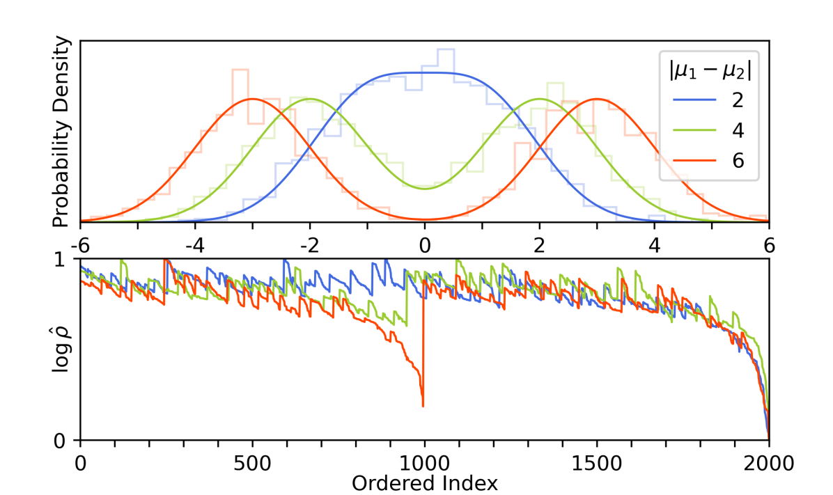
Figure 3: Examples of ordered-density plots (bottom) generated by AstroLink (using default settings) for three $1$-dimensional data sets that have been randomly sampled from two standard normal distributions with varying separations between them (top). We can see that as the separation grows, it becomes easier to distinguish the two distributions as individual clusters.

The ordered-density plot reveals the input data points linked by decreasing density and based on their shared neighbourhood connectivity. Peaks in the plot represent overdensities as the points within them are both denser than their surrounds and ordered consecutively due to being locally connectable to each other. Fig. 3 portrays two main peaks that become increasingly prominent as the separation between the distributions grows. Within these peaks are a series of smaller peaks that correspond to the stochastic clumping that arises whenever a data set contains spatial randomness – as is the case here due to the data sets being created via random sampling. As the distribution separation increases, these smaller peaks become far less prominent than the two main peaks which indicates that a set of meaningful clusters is identifiable using the ordered-density plot.

3.4.4 The Merger Tree

The hierarchies of the subgroups ($G$) and of the complementary groups ($G_{\mathrm{comp}}$) are also generated during the aggregation process. For every subgroup there is exactly one (larger) complementary group, as these two groups are merged whenever a saddle point in the density field is found during the aggregation process. An example of these two components can be seen in Fig. 4.

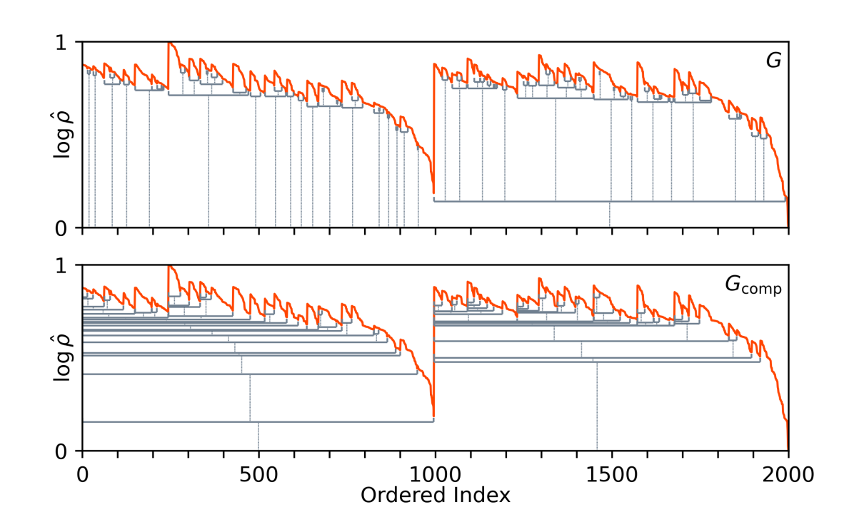
Figure 4: The AstroLink merger tree and its relation to the ordered-density plot for the $1$-dimensional data set with the largest separation from Fig. 3. The grey markings denote the subgroups, $G$ (top), and their complementary groups, $G_{\mathrm{comp}}$ (bottom), found during the aggregation process.

The subgroup hierarchy is akin to that of the SUBFIND (Springel et al., 2001) and EnLink (Sharma & Johnston, 2009) algorithms. While this is suitable for some clustering scenarios, as evident in Fig. 4, it alone can only capture one of the two standard normal distributions. Thus, in many scenarios, the complementary group hierarchy is essential for identifying all relevant clusters. As such, AstroLink uses it to correct the final cluster hierarchy so that it meets some basic expectations – refer to Sec. 3.5.4 for details on this correction.

3.5 Identifying Clusters

AstroLink now identifies clusters by assessing the statistical distinctiveness of groups from the merger tree within the ordered-density plot. By measuring the clusteredness of each group and fitting a model to the distribution of this measure for all subgroups, subgroups are then classified as inliers (noise) or outliers (clusters) from this distribution. An optional hierarchy correction can then also be performed by incorporating the complementary groups that correspond to the identified clusters.

3.5.1 The Clusteredness of a Group

Intuitively, the measure of a group’s clusteredness should consider its overdensity and also account for the magnitude of intra-group noise. Due to the logarithmic scaling of densities from Eq. 2, vertical differences on the ordered-density plot represent the logarithm of a ratio of densities. As such, we can calculate the logarithm of a group’s overdensity factor by finding the difference between some characteristic $\log\hat{\rho}$ value of that group and the $\log\hat{\rho}$ value of its surrounds. The $\log\hat{\rho}$ value at its surrounds is taken as the $\log\hat{\rho}$ saddle-point that was used to merge the group into the merger tree – which is the maximum $\log\hat{\rho}$ that can be found at the group’s boundary. The group’s characteristic $\log\hat{\rho}$ value is taken to be maximum $\log\hat{\rho}$ found within the group minus a measure of the intra-group noise. As such, we construct a statistical measure of clusteredness, which we call the prominence, such that for any group, $g$;

$$\mathcal{P}_{g}=\log\hat{\rho}_{\mathrm{max},g}-\log\hat{\rho}_{\mathrm{boundary},g}-\log\hat{\rho}_{\mathrm{noise,g}}.$$ (3)

Here $\log\hat{\rho}_{\mathrm{max},g}$ is the maximum value of $\log\hat{\rho}$ within $g$, $\log\hat{\rho}_{\mathrm{boundary},g}$ is the value of $\log\hat{\rho}$ at the saddle point that connects that $g$ to another, and $\log\hat{\rho}_{\mathrm{noise,g}}$ is a term that accounts for intra-group noise. The noise-correction term is calculated as the root-mean-square of the $\log\hat{\rho}_{\mathrm{max},\mathrm{child}}-\log\hat{\rho}_{\mathrm{boundary},\mathrm{child}}$ values for each of the direct children (excluding children of children) subgroups of $g$. As such, this measure is akin to the logarithm of a signal to noise ratio. The top panel of Fig. 5 shows a visualisation of the calculation of $\mathcal{P}_{g}$ for the largest subgroup shown in Fig. 4.

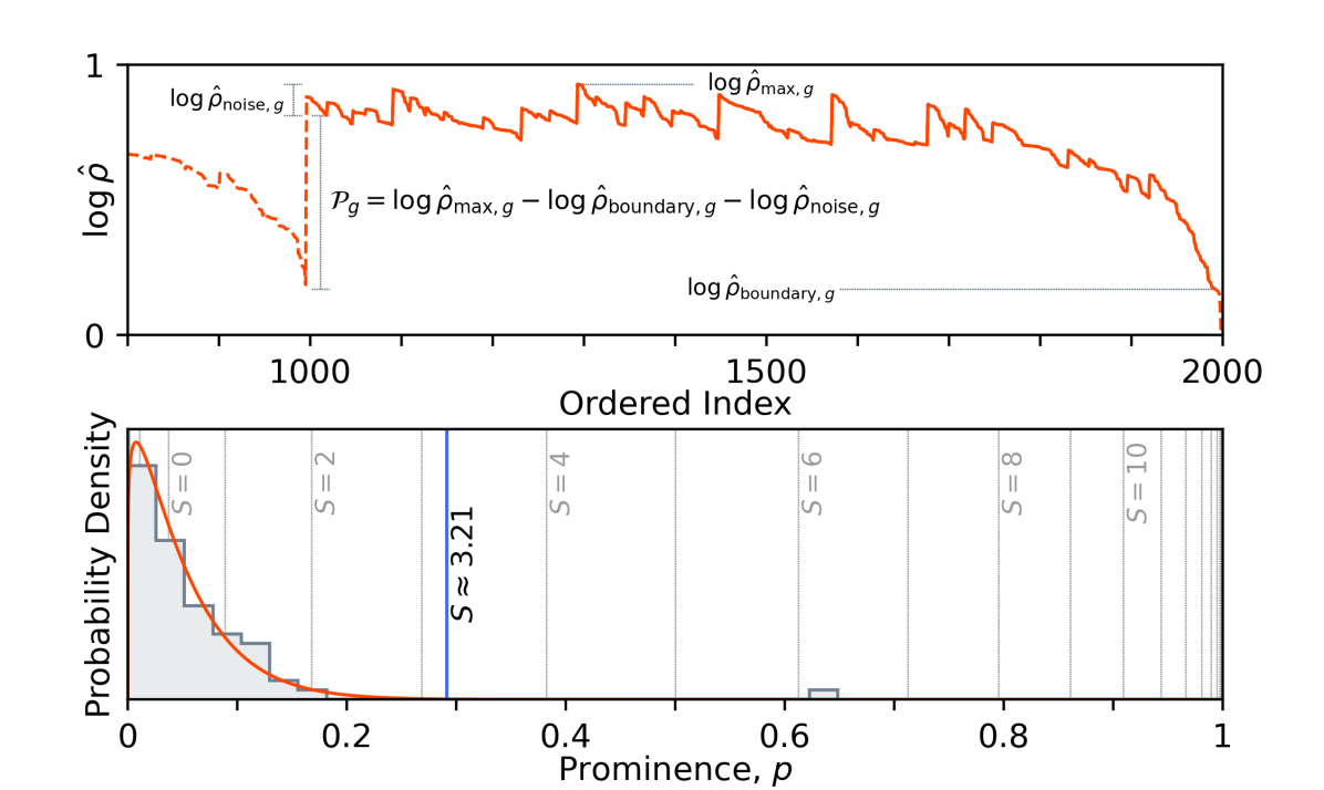
Figure 5: An illustration of the prominence calculation (top) for the largest subgroup and the resulting prominence distribution (bottom) for all subgroups (subgroups are shown in Fig. 4). The largest subgroup is objectively more clustered, and hence is a clear outlier ($S>6$), from the other subgroups. The solid red line indicates the model for subgroup prominences (detailed in Sec. 3.5.2) and the solid blue line, positioned at $p=c$, is labelled with the corresponding data-driven estimate of $S$ (detailed in Sec. 3.5.3).

3.5.2 A Model for Subgroup Prominences

AstroLink now fits a descriptive model, $M$, on a case-by-case basis to the prominences of the subgroups by minimising the corresponding negative log-likelihood. For density estimates of Poisson noise computed with a fixed number of nearest neighbours, the probability distribution of $\rho$ should be approximately Gaussian (Sharma & Johnston, 2009). As such, the prominence (which is effectively an absolute difference of these estimates) should belong to a half-normal distribution. With real data however, some critical assumptions are violated; i.e. generally the nearest neighbours are not drawn from homogeneous Poisson noise; the density estimation and aggregation processes impose small-scale smoothing effects on the density field that suppress the production of groups with fewer points than $N_{k_{\mathrm{den}}}$ and $N_{k_{\mathrm{link}}}$ respectively; etc. As such, we construct $M$ to be a combination of two probability distributions – one for noise and one for clusters – such that $M(p)=H(c-p)M_{\mathrm{noise}}(p)+H(p-c)M_{\mathrm{clusters}}(p)$ where $p$ is a random variable representing prominence, $H(x)$ is the Heaviside step function, and $c\in[0,1]$ is a parameter of the model.

For $M_{\mathrm{noise}}$, we have used the second-order correction estimate of the Akaike information criterion (AIC & AICc; Akaike, 1974; Hurvich & Tsai, 1989) and the Bayesian information criterion (BIC; Schwarz, 1978) to assess the suitability of the Log-Normal, Inverse Gaussian, Gamma, Beta, Beta-Prime, Generalised Gamma, and Generalised Beta-Prime distributions when AstroLink is applied to a range of $n$-point $d$-dimensional uniform distributions on the unit hypercube (for various combinations of $n$ and $d$). With both criteria, we found that using the Beta distribution for $M_{\mathrm{noise}}$ is best (with parameters $a,b\geq 1$ and typically $b\gg a$, i.e. uni-modal with a positively-skewed tail). We also found that using a Uniform distribution for $M_{\mathrm{clusters}}$ provides enough shape flexibility so that $M_{\mathrm{noise}}$ remains largely unaffected by the presence of outliers. This can be seen in the bottom panel of Fig. 5 as the presence of a $S>6$ outlier does not detract from the fitting-quality of $M_{\mathrm{noise}}$. Using the model parameters ($a,b,c$), $M_{\mathrm{noise}}(p)$ and $M_{\mathrm{clusters}}(p)$ are also weighted so that $M(p)$ is normalised and continuous on the interval $p\in[0,1]$.

Figure 6: Clusters identified from the toy example of Fig. 3 using AstroLink with default settings. Shown here is the $1$-dimensional probability distribution alongside the input data that was sampled from it (top) and the ordered-density plot, the final hierarchy tree, and the clusters’ significances (bottom). This data is coloured according to the cluster that it has been allocated to by AstroLink. AstroLink has differentiated the two Gaussian distributions from the noisy density fluctuations within them with a statistical significance of $7.24\sigma_{\mathrm{noise}}$ and $6.28\sigma_{\mathrm{noise}}$ respectively.

3.5.3 The Statistical Significance of Clusters

To label subgroups as clusters, AstroLink now simply identifies all subgroups that have a statistical significance ($\mathcal{S}$) that is greater than $S\sigma_{\mathrm{noise}}$. To be clear, any subgroup ($g$) will now be labelled as a cluster if its prominence ($\mathcal{P}_{g}$) satisfies

$$\mathcal{S}_{g}\coloneq{F_{\mathcal{N}(0,1)}}^{-1}\left[F_{\beta(a,b)}(\mathcal{P}_{g})\right]\geq S,$$ (4)

where $F_{\mathcal{N}(0,1)}$ and $F_{\beta(a,b)}$ are the standard normal and Beta cumulative distribution functions respectively. The parameters $a$ and $b$ are derived by fitting the model outlined in Sec. 3.5.2 to the distribution of subgroup prominences. With this, the subgroup prominences are transformed so that the subgroup significances follow a standard normal with a long positive tail of outliers containing the significances of increasingly more clustered subgroups. The $S$ parameter is therefore a measure of how clustered – relative to the noise present within the data – the resultant clusters are. The value of $S$ may be chosen by the user but the default value is $S=auto$, in which case AstroLink calculates it according to the model parameter, $c$, i.e. $S={F_{\mathcal{N}(0,1)}}^{-1}\left[F_{\beta(a,b)}(c)\right]$. Since $c$ marks the prominence value for which the subgroups transition from noise to clusters, it can therefore be used to automatically estimate an appropriate value for $S$.

3.5.4 Correcting the Hierarchy

To ensure all relevant clusters are included in the final hierarchy, AstroLink can optionally label the complementary groups as clusters as well as those from the subgroups. If $h\_style=1$ (default), then for each cluster already found it’s complementary group is considered if it also satisfies Eq. 4. Then for each of these cluster-like complementary groups, AstroLink labels it a cluster if it is the smallest cluster-like complementary group that shares its starting position within the ordered list, $O$. The latter condition simplifies and reduces the depth of the resultant hierarchy by eliminating clusters-within-clusters that only differ by a small number of points. With these additional clusters the resultant hierarchy is similarly styled to CluSTAR-ND, however now each cluster is a more meaningful and statistically interpretable group. Fig. 6 now depicts the final hierarchy of clusters extracted from the same toy data set shown in Figs. 3 – 5. This step can be ignored by setting $h\_style=0$.

4 Performance Analysis

We now assess the performance of AstroLink by applying it to a series of synthetic galaxies each with a set of ground-truth labels. We analyse the time and space complexity of AstroLink as well as it’s ability to produce a meaningful set of astrophysical clusters in comparison to its algorithmic predecessors – CluSTAR-ND and Halo-OPTICS. Lastly, we show some of these outputs visually.

4.1 Synthetic Data

To assess AstroLink’s performance we use Galaxia (Sharma et al., 2011) to produce random samples of the $11$ $\Lambda$CDM stellar haloes from Bullock & Johnston (2005) and the complementary $6$ artificial stellar haloes from Johnston et al. (2008). Each of the original $\Lambda$CDM stellar haloes are simulated using a hybrid semi-analytical and hydrodynamic $N$-body approach. Satellites are first modelled as $N$-body dark matter systems within a parent galaxy whose disk, bulge, and halo are defined by time dependent semi-analytic functions. The simulation uses a $\Lambda$CDM cosmology with parameters $\Omega_{m}=0.3$, $\Omega_{\Lambda}=0.7$, $\Omega_{b}h^{2}=0.024$, $h=0.7$, and $\sigma_{8}=0.9$. Semi-analytical models then assign stellar populations to each satellite while a chemical enrichment model (Robertson et al., 2005; Font et al., 2006) calculates age-appropriate metallicities for the star particles. This process yields satellites whose structural properties are in agreement with the Local Group’s dwarf galaxies.

With this regime each satellite has three main model parameters; the time since accretion ($t_{\mathrm{acc}}$), the luminosity ($L_{\mathrm{sat}}$), and the orbital circularity ($\epsilon=J/J_{\mathrm{circ}}$). The distribution of these parameters specify the accretion history of a halo and as such a further $6$ artificial haloes were created in Johnston et al. (2008) for the purpose of studying the effects of different accretion histories on the properties of haloes. These $6$ artificial haloes are characterised by accretion histories that are predominantly radial ($\epsilon<0.2$); circular ($\epsilon>0.7$); old ($t_{\mathrm{acc}}>11$ Gyr); young ($t_{\mathrm{acc}}<8$ Gyr); high luminosity ($L_{\mathrm{sat}}>10^{7}L_{\mathrm{\odot}}$); and low luminosity ($L_{\mathrm{sat}}<10^{7}L_{\mathrm{\odot}}$).

For these galaxies, Galaxia provides spatial (${\bf x}=(x,y,z)$), kinematic (${\bf v}=(v_{x},v_{y},v_{z})$), and chemical (${\bf m}=($[Fe/H],[$\alpha$/Fe]$)$) quantities for each particle, along with ground-truth labels indicating the particle’s satellite of origin and also whether each satellite is self-bound. More details on these simulations can be found in Sec. 3.4 of Sharma et al. (2011) and references therein. With this information, we apply AstroLink to the various galaxies and assess its performance.

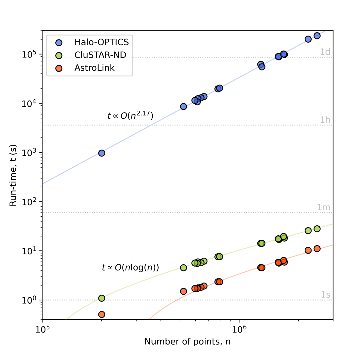
Figure 7: The run-times and time-complexities of AstroLink, CluSTAR-ND, and Halo-OPTICS when applied to the spatial positions ($\bf{x}$) of particles within the synthetic galaxies from Galaxia. The curves of best fit correspond to the time complexities for the algorithms. AstroLink and CluSTAR-ND both exhibit a run-time improvement of many orders of magnitude over Halo-OPTICS, and even though their time complexities are the same, AstroLink’s smaller constant factor means that (asymptotically) it is an additional $\sim 3$ times faster than CluSTAR-ND. Furthermore, since AstroLink may be run in parallel for a larger portion of its computation, it is the most-suitable of the three algorithms for applications to large data sets.

4.2 Time Complexity

We now compare the run-time of AstroLink to that of CluSTAR-ND and Halo-OPTICS. Fig. 7 shows the run-times of the three algorithms when applied to the spatial positions of the synthetic galaxies from Galaxia. All runs were performed using a single CPU and all codes are written using Python3 – each making use of optimised numerical packages such as NumPy (Harris et al., 2020), SciPy (Virtanen et al., 2020), Scikit-learn (Pedregosa et al., 2011), and Numba (AstroLink & CluSTAR-ND only; Lam et al., 2015) to differing degrees.

It is clear from Fig. 7 that AstroLink outperforms its predecessors in terms of running time. The time complexities of AstroLink and CluSTAR-ND are $\mathcal{O}(n\mathrm{log}(n))$ while Halo-OPTICS exhibits super-quadratic time complexity at $\mathcal{O}(n^{2.17})$. For Halo-OPTICS, this results from a combination of it performing a radial search about every data point and that the cuspyness of the haloes increase with their size – this is discussed further in Oliver et al. (2022). This does not impact AstroLink or CluSTAR-ND, as they only perform a $k_{\mathrm{den}}$ nearest neighbour search for each data point. While this $k_{\mathrm{den}}$ nearest neighbour search still contributes the largest portion of their total run-time.

These run-times can be further improved by using multiple CPUs in parallel. For AstroLink, all steps are parallelised over over shared memory – except the part of the aggregation process resembling Kruskal’s MST. However, the majority of the computation in this step can also be parallelised (Bader & Cong, 2006) by combining Prim’s MST algorithm (Jarník, 1930; Prim, 1957; Dijkstra, 2022) Boruvska’s MST algorithm (Borůvka, 1926; Choquet, 1938; Sollin, 1965) – an implementation we leave as future work.

4.3 Space Complexity

In terms of memory footprint, each algorithm has $O(n)$ space complexity, although with differing constant factors. CluSTAR-ND has the largest of these factors since it stores lists of indices for each cluster, while AstroLink and Halo-OPTICS compute an ordered list and then only store the start and end positions of each cluster within this list. Conversely, Halo-OPTICS has the smallest constant factor, as it only stores indices of the radial nearest neighbours for one point at a time – whereas AstroLink and CluSTAR-ND keep copies of the $k_{\mathrm{den}}$ nearest neighbours of every point. Consequently, AstroLink boasts the median constant factor and thus it presents a trade-off between time and space complexity while improving interpretability and reliability.

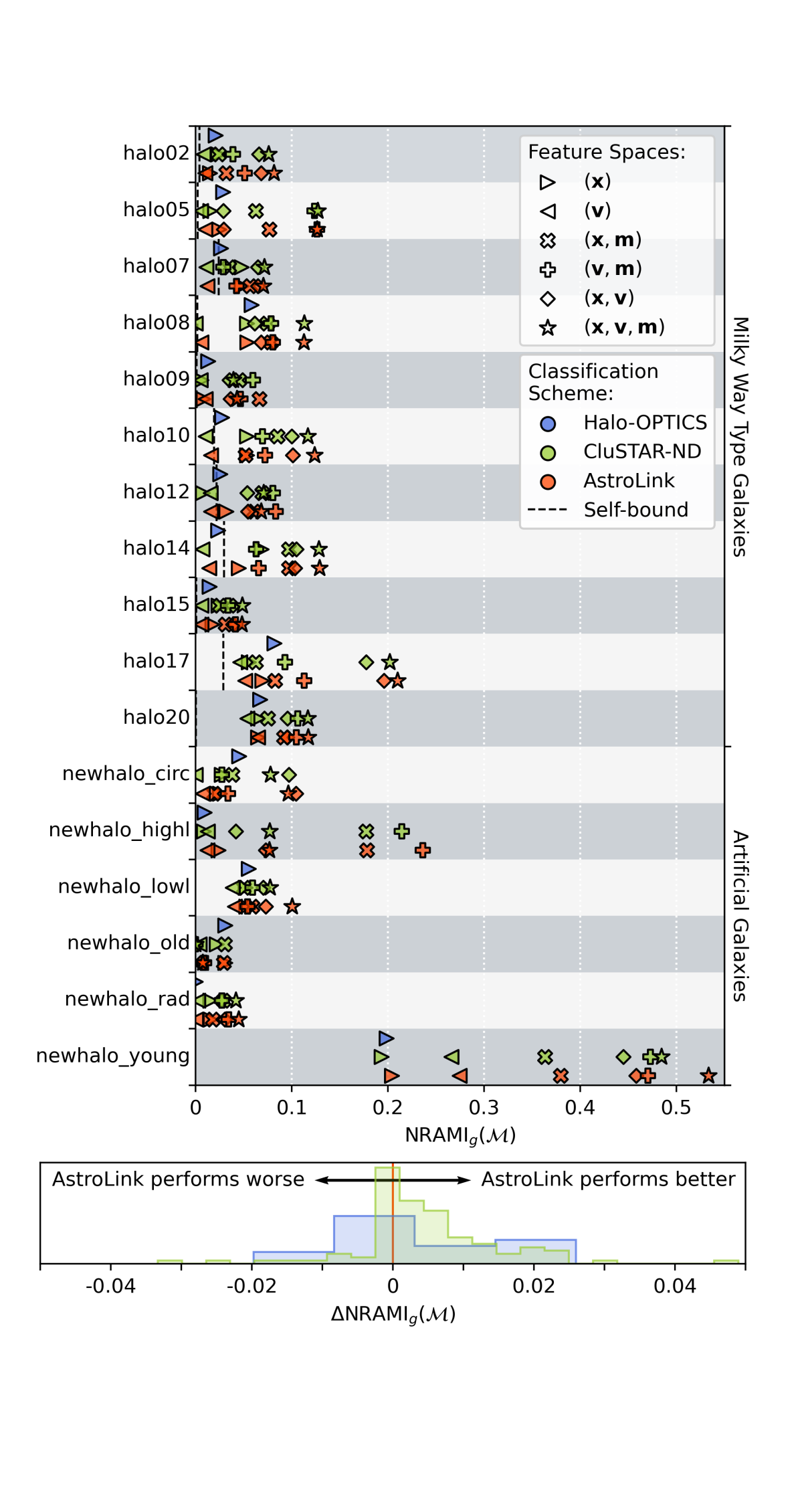
Figure 8: The NRAMI between for the AstroLink, CluSTAR-ND, and Halo-OPTICS algorithms when applied to each synthetic galaxy and feature space combination (top) and the differences in the NRAMI between the AstroLink algorithm and its predecessors for each of these clustering scenarios (bottom). The NRAMI of a hypothetical set of clusterings that exactly classify the self-bound satellites within each MW type galaxy are also shown in the top panel as a reference. AstroLink outperforms CluSTAR-ND in $\sim 75\%$ of comparisons and Halo-OPTICS in $\sim 50\%$ of comparisons.

4.4 Clustering Power

We now assess the capability of AstroLink to retrieve a set of astrophysical clusters in comparison to CluSTAR-ND and Halo-OPTICS. We first define an information-based statistic that represents the portion of meaningful classification that has been made by the algorithms, we then run each algorithm over the synthetic galaxies, before finally comparing their outputs.

4.4.1 Measuring Clustering Power

We use the normalised random-adjusted mutual-information presented (NRAMI) in Sec. 5.1.1 of Oliver et al. (2022) to assess the goodness-of-fit between a clustering ($C_{g}$) produced by AstroLink/CluSTAR-ND/Halo-OPTICS and the ground-truth labels ($T_{g}$) provided by Galaxia for a given galaxy $g$. To prepare the hierarchy of clusters from these algorithms for comparison to the flat ground-truth labels, we first assign a unique label to every point of the input data that corresponds to the smallest cluster that it is predicted to be a part of – we refer to this flattened set of labels as $C_{g}^{*}$. The knowledge gained about a galaxy’s satellites from a clustering algorithm can then be quantified by the mutual information (Shannon, 1948) between $C_{g}^{*}$ and $T_{g}$, such that

$$I(C_{g}^{*};T_{g})=H(T_{g})-H(C_{g}^{*}|T_{g}),\ \mathrm{where}$$

$$H(T_{g})\equiv-\sum_{t\in T_{g}}P(t)\ \mathrm{log}(P(t)),\ \mathrm{and}$$

$$H(C_{g}^{*}|T_{g})\equiv-\sum_{c\in C_{g}^{*},\ t\in T_{g}}P(c,t)\ \mathrm{log}\bigg{(}\frac{P(c,t)}{P(t)}\bigg{)}.$$ (5)

Here $H(T_{g})$ is the entropy of $T_{g}$ and $H(C_{g}^{*}|T_{g})$ is the conditional entropy of $C_{g}^{*}$ given $T_{g}$. The portion of relevant information learnt can then be calculated by normalising this to ensure that the expected knowledge gained about $T_{g}$ from a random re-clustering of $C_{g}^{*}$ (i.e. a set of randomly assigned labels with equal sizes as those in $C_{g}^{*}$) is represented by a value of $0$, and that similarly, the knowledge gained from a perfect clustering ($C_{g}^{*}=T_{g}$) is represented by a value of $1$. Hence, if $\mathcal{M}$ represents some feature space combination upon which the predicted clusters are dependent, the measure we use to assess an algorithm’s clustering power is defined as

$$\mathrm{NRAMI}_{g}(\mathcal{M})=\frac{I(C_{g}^{*}(\mathcal{M});T_{g})-E[I(R_{g}^{*}(\mathcal{M});T_{g})]}{H(T_{g})-E[I(R_{g}^{*}(\mathcal{M});T_{g})]},$$ (6)

where $E[I(R_{g}^{*}(\mathcal{M});T_{g})]$ is the expected mutual information between a random re-clustering, $R_{g}^{*}(\mathcal{M})$, and $T_{g}$. Refer to Sec. 5.1.1 of Oliver et al. (2022) for more details on this measure.

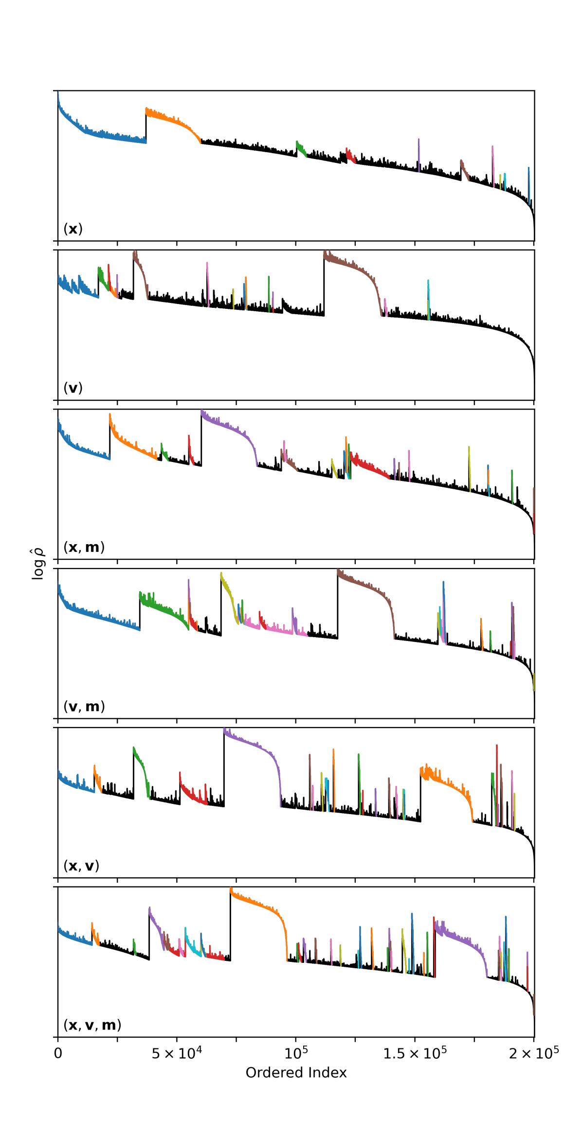
Figure 9: Ordered density plots produced by AstroLink when applied to the artificial galaxy, newhalo_young, over various feature space combinations. Clusters are represented with a colour cycle of nine colours (also depicted in Fig. 10) and have been identified with AstroLink’s default settings (unlike in Fig. 8, $S$ is now estimated from the data)

.

Figure 10: Illustrations of the spatial positions of clusters found by applying AstroLink to the artificial galaxy, newhalo_young, over various feature spaces. Clusters found by AstroLink are shown with the same colours as in the ordered-density plots of Fig. 9.

4.4.2 Comparison

We now compare each algorithm’s clustering power by applying them to each synthetic galaxy over various combinations of the available feature space. We select $\mathcal{M}$ from the combinations of the spatial (${\bf x}$), kinematic (${\bf v}$), and chemical (${\bf m}$) feature spaces, i.e. $({\bf x})$, $({\bf v})$, $({\bf x},{\bf m})$, $({\bf v},{\bf m})$, $({\bf x},{\bf v})$, and $({\bf x},{\bf v},{\bf m})$. We apply CluSTAR-ND and Halo-OPTICS using their default settings (refer to Oliver et al., 2022), but since their cluster extraction parameters have been optimised for these galaxies we alter the significance threshold parameter, $S$, of AstroLink in this comparison.

For values of $S$ in the range of $\sim 3$ to $\sim 6$, the NRAMI between the AstroLink output and the ground-truth hovers around values that are consistent with the CluSTAR-ND output. By default ($S=auto$), the data-driven value of $S$ falls within this range for all clustering scenarios – and so naively one can expect to achieve a roughly equal clustering power when using AstroLink’s default settings. However since the output of AstroLink is more easily interpretable and the significance parameter is intuitive to adjust, we set the $S$ parameter on a case-by-case basis in order to produce the best possible value of the $\mathrm{NRAMI}_{g}(\mathcal{M})$. This allows us to see what AstroLink is realistically capable of achieving in a practical use-case/data-exploration scenario.

Fig. 8 depicts the clustering performance of each algorithm when applied to each galaxy and feature space combination as well as the difference in clustering power for each algorithm. Here AstroLink is shown to generally outperform the other algorithms, and even when it does not, the difference is most-often negligible. It is also important to note that AstroLink is effectively being penalised by the NRAMI measure – since it tends to produce a shallower hierarchy than the other two codes. With fewer levels to the hierarchy there are fewer groupings at high densities which improves the interpretability of the AstroLink output but in this case imposes a penalty to AstroLink in this comparison. Within this figure, it can also be noted that if the feature space of the input data has a larger number of more informative dimensions then the clustering power will generally be improved. Additionally, the type of clusters within the galaxy has a large effect on the clustering power – young or high luminosity satellites are well-matched whereas those that are old or that are orbiting on predominantly radial trajectories are more difficult to recover.

4.5 Visualising Clustering Structure

We now also visually present the AstroLink output in order to further demonstrate its performance and usability. The ordered-density plot produced by AstroLink holds the information attainable from the estimated density field, so in Fig. 9 we illustrate how this information varies for the predominantly young artificial galaxy from Johnston et al. (2008) when using different feature spaces to find the clustering of the data. Here it can be seen that the complexity of the clustering structure increases with the number of informative dimensions and hence visualising the ordered-density plot provides valuable insight to the user. Furthermore, the ordered-density plot can be used as a guide to the user when fine-tuning the significance threshold ($S$) – as unclassified structure can be classified by lowering $S$ and, vice versa, classified noise can be declassified by raising $S$.

Fig. 10 depicts the spatial distributions of those clusters shown coloured in the corresponding ordered density plots of Fig. 9. Each panel gives an indication as to which types of clusters AstroLink can retrieve given that the input data is expressed through certain feature space combinations. We see here that spatially compact clusters are best described by spatial features, stream-like clusters are best described by kinematic and chemical features, and combining these feature sets tends to give good results for various cluster types – permitting their retrieval simultaneously. Notably, the addition of chemical abundances to the input data’s feature space gives AstroLink more knowledge about otherwise phase-mixed clusters. These observations agree with theoretical and intuitive predictions about how one would expect a generalised astrophysical clustering algorithm to perform.

5 Conclusions

We have presented AstroLink, a generalised astrophysical clustering algorithm that produces a set of arbitrarily-shaped hierarchical clusters from an arbitrarily-shaped point-based data set such that the clusters found are statistical outliers from noisy density fluctuations. The algorithm is unsupervised, requires little to no input from the user (other than the trivial requirement to supply the data), and has an intuitive set of hyperparameters that can be quickly and intuitively adjusted to ensure that the resulting clusters meet the user’s needs.

We have also demonstrated the robustness of AstroLink’s performance in comparison to its predecessors, CluSTAR-ND and Halo-OPTICS. We find that AstroLink classifies satellites from simulated galaxies with greater accuracy while requiring less run-time and memory allocation. Similarly to Halo-OPTICS, it also produces a visual representation of the input data’s implicit clustering structure. However unlike Halo-OPTICS, the ordered-density plot is determinable and more easily interpretable – owing to the fact that absolute vertical differences correspond directly to overdensity factors.

While there are still ways to improve AstroLink’s output (e.g. defining a locally-adaptive metric before estimating density, propagating data point uncertainties into cluster uncertainties, using an supplementary model-based approach that attributes additional data points to the AstroLink clusters, etc.). AstroLink is well-suited to the clustering problem of finding astrophysically relevant groups from large-scale data sets in both simulated and observational settings.

Data Availability

The data underlying this article may be made available on reasonable request to the corresponding author. The AstroLink code will be made available on GitHub upon acceptance of this paper.

References

- Akaike (1974) Akaike H., 1974, IEEE transactions on automatic control, 19, 716
- Ankerst et al. (1999) Ankerst M., Breunig M. M., Kriegel H.-P., Sander J., 1999, in ACM Sigmod record. ACM, pp 49–60, doi:10.1145/304182.304187
- Avila et al. (2014) Avila S., et al., 2014, Monthly Notices of the Royal Astronomical Society, 441, 3488
- Bader & Cong (2006) Bader D. A., Cong G., 2006, Journal of Parallel and Distributed Computing, 66, 1366
- Behroozi et al. (2012) Behroozi P. S., Wechsler R. H., Wu H.-Y., 2012, The Astrophysical Journal, 762, 109
- Behroozi et al. (2015) Behroozi P., et al., 2015, Monthly Notices of the Royal Astronomical Society, 454, 3020
- Borůvka (1926) Borůvka O., 1926, O jistém problému minimálním
- Breunig et al. (1999) Breunig M. M., Kriegel H.-P., Ng R. T., Sander J., 1999. Principles of Data Mining and Knowledge Discovery. Springer Berlin Heidelberg, pp 262–270, doi:10.1145/342009.335388
- Bullock & Johnston (2005) Bullock J. S., Johnston K. V., 2005, The Astrophysical Journal, 635, 931
- Campello et al. (2015) Campello R. J. G. B., Moulavi D., Zimek A., Sander J., 2015, ACM Trans. Knowl. Discov. Data, 10
- Canovas et al. (2019) Canovas H., et al., 2019, A&A, 626
- Casamiquela et al. (2022) Casamiquela L., et al., 2022, arXiv preprint arXiv:2206.03777
- Choquet (1938) Choquet G., 1938, Comptes Rendus Hebdomadaires des Séances de l’Académie des Sciences, 206, 310
- Costado et al. (2016) Costado M. T., Alfaro E. J., González M., Sampedro L., 2016, Monthly Notices of the Royal Astronomical Society, 465, 3879
- Davis et al. (1985) Davis M., Efstathiou G., Frenk C. S., White S. D., 1985, The Astrophysical Journal, 292, 371
- Diemand et al. (2006) Diemand J., Kuhlen M., Madau P., 2006, The Astrophysical Journal, 649, 1
- Dijkstra (2022) Dijkstra E. W., 2022, in , Edsger Wybe Dijkstra: His Life, Work, and Legacy. pp 287–290
- Elahi et al. (2013) Elahi P. J., et al., 2013, Monthly Notices of the Royal Astronomical Society, 433, 1537
- Elahi et al. (2019) Elahi P. J., Canas R., Poulton R. J. J., Tobar R. J., Willis J. S., Lagos C. d. P., Power C., Robotham A. S. G., 2019, Publications of the Astronomical Society of Australia, 36, e021
- Epanechnikov (1969) Epanechnikov V. A., 1969, Theory of Probability & Its Applications, 14, 153
- Ester et al. (1996) Ester M., Kriegel H.-P., Sander J., Xu X., 1996, in Kdd. pp 226–231
- Font et al. (2006) Font A. S., Johnston K. V., Bullock J. S., Robertson B. E., 2006, The Astrophysical Journal, 638, 585
- Fuentes et al. (2017) Fuentes S. S., De Ridder J., Debosscher J., 2017, Astronomy & Astrophysics, 599, A143
- Giocoli et al. (2008) Giocoli C., Tormen G., van den Bosch F. C., 2008, MNRAS, 386, 2135
- Hadzhiyska et al. (2021) Hadzhiyska B., Eisenstein D., Bose S., Garrison L. H., Maksimova N., 2021, Monthly Notices of the Royal Astronomical Society, 509, 501
- Han et al. (2017) Han J., Cole S., Frenk C. S., Benitez-Llambay A., Helly J., 2017, Monthly Notices of the Royal Astronomical Society, 474, 604
- Harris et al. (2020) Harris C. R., et al., 2020, Nature, 585, 357
- Higgs et al. (2021) Higgs C., McConnachie A., Annau N., Irwin M., Battaglia G., Côté P., Lewis G., Venn K., 2021, Monthly Notices of the Royal Astronomical Society, 503, 176
- Hurvich & Tsai (1989) Hurvich C. M., Tsai C.-L., 1989, Biometrika, 76, 297
- Jarník (1930) Jarník V., 1930, O jistém problému minimálním.(Z dopisu panu O. Borůvkovi)
- Jayasinghe et al. (2019) Jayasinghe T., et al., 2019, Monthly Notices of the Royal Astronomical Society, 488, 1141
- Jensen et al. (2021) Jensen J., et al., 2021, Monthly Notices of the Royal Astronomical Society, 507, 1923
- Johnston et al. (1996) Johnston K. V., Hernquist L., Bolte M., 1996, ApJ, 465, 278
- Johnston et al. (2008) Johnston K. V., Bullock J. S., Sharma S., Font A., Robertson B. E., Leitner S. N., 2008, The Astrophysical Journal, 689, 936
- Kamdar et al. (2021) Kamdar H., Conroy C., Ting Y.-S., 2021, arXiv preprint arXiv:2106.02050
- Knebe et al. (2011) Knebe A., et al., 2011, Monthly Notices of the Royal Astronomical Society, 415, 2293
- Knebe et al. (2013) Knebe A., et al., 2013, Monthly Notices of the Royal Astronomical Society, 428, 2039
- Knollmann & Knebe (2009) Knollmann S. R., Knebe A., 2009, ApJS, 182, 608
- Koppelman et al. (2019) Koppelman H. H., Helmi A., Massari D., Price-Whelan A. M., Starkenburg T. K., 2019, Astronomy & Astrophysics, 631, L9
- Kounkel & Covey (2019) Kounkel M., Covey K., 2019, The Astronomical Journal, 158, 122
- Kruskal (1956) Kruskal J. B., 1956, Proceedings of the American Mathematical society, 7, 48
- Lam et al. (2015) Lam S. K., Pitrou A., Seibert S., 2015, in Proceedings of the Second Workshop on the LLVM Compiler Infrastructure in HPC. pp 1–6
- Lee et al. (2014) Lee J., et al., 2014, Monthly Notices of the Royal Astronomical Society, 445, 4197
- Lövdal et al. (2022) Lövdal S. S., Ruiz-Lara T., Koppelman H. H., Matsuno T., Dodd E., Helmi A., 2022, arXiv preprint arXiv:2201.02404
- Maciejewski et al. (2009) Maciejewski M., Colombi S., Springel V., Alard C., Bouchet F. R., 2009, MNRAS, 396, 1329
- Mahajan et al. (2018) Mahajan S., Singh A., Shobhana D., 2018, Monthly Notices of the Royal Astronomical Society, 478, 4336
- Mahalanobis (1936) Mahalanobis P. C., 1936.
- Malhan & Ibata (2018) Malhan K., Ibata R. A., 2018, Monthly Notices of the Royal Astronomical Society, 477, 4063
- Massaro et al. (2019) Massaro F., Alvarez-Crespo N., Capetti A., Baldi R., Pillitteri I., Campana R., Paggi A., 2019, The Astrophysical Journal Supplement Series, 240, 20
- Mateu et al. (2011) Mateu C., Bruzual G., Aguilar L., Brown A. G. A., Valenzuela O., Carigi L., Velázquez H., Hernández F., 2011, Monthly Notices of the Royal Astronomical Society, 415, 214
- Mateu et al. (2017) Mateu C., Read J. I., Kawata D., 2017, Monthly Notices of the Royal Astronomical Society, 474, 4112
- McConnachie et al. (2018) McConnachie A. W., et al., 2018, The Astrophysical Journal, 868, 55
- McInnes et al. (2017) McInnes L., Healy J., Astels S., 2017, Journal of Open Source Software, 2, 205
- Oliver et al. (2021) Oliver W. H., Elahi P. J., Lewis G. F., Power C., 2021, Monthly Notices of the Royal Astronomical Society, 501, 4420
- Oliver et al. (2022) Oliver W. H., Elahi P. J., Lewis G. F., 2022, Monthly Notices of the Royal Astronomical Society, 514, 5767
- Onions et al. (2012) Onions J., et al., 2012, Monthly Notices of the Royal Astronomical Society, 423, 1200
- Onions et al. (2013) Onions J., et al., 2013, Monthly Notices of the Royal Astronomical Society, 429, 2739
- Pearson et al. (2022) Pearson S., Clark S. E., Demirjian A. J., Johnston K. V., Ness M. K., Starkenburg T. K., Williams B. F., Ibata R. A., 2022, The Astrophysical Journal, 926, 166
- Pedregosa et al. (2011) Pedregosa F., et al., 2011, Journal of Machine Learning Research, 12, 2825
- Press & Schechter (1974) Press W. H., Schechter P., 1974, The Astrophysical Journal, 187, 425
- Prim (1957) Prim R. C., 1957, Bell System Technical Journal, 36, 1389
- Robertson et al. (2005) Robertson B., Bullock J. S., Font A. S., Johnston K. V., Hernquist L., 2005, The Astrophysical Journal, 632, 872
- Ruiz et al. (2018) Ruiz A., Corral A., Mountrichas G., Georgantopoulos I., 2018, Astronomy & Astrophysics, 618, A52
- Sain (2002) Sain S. R., 2002, Computational Statistics & Data Analysis, 39, 165
- Sander et al. (2003) Sander J., Qin X., Lu Z., Niu N., Kovarsky A., 2003, in Whang K.-Y., Jeon J., Shim K., Srivastava J., eds, Advances in Knowledge Discovery and Data Mining. Springer Berlin Heidelberg, pp 75–87
- Schwarz (1978) Schwarz G., 1978, The annals of statistics, pp 461–464
- Shannon (1948) Shannon C. E., 1948, The Bell System Technical Journal, 27, 379
- Sharma & Johnston (2009) Sharma S., Johnston K. V., 2009, The Astrophysical Journal, 703, 1061
- Sharma et al. (2011) Sharma S., Bland-Hawthorn J., Johnston K. V., Binney J., 2011, The Astrophysical Journal, 730, 3
- Shih et al. (2021) Shih D., Buckley M. R., Necib L., Tamanas J., 2021, Monthly Notices of the Royal Astronomical Society, 509, 5992
- Sollin (1965) Sollin M., 1965, Programming, Games, and Transportation Networks
- Soto et al. (2022) Soto M., et al., 2022, Monthly Notices of the Royal Astronomical Society, 513, 2747
- Springel et al. (2001) Springel V., White S. D. M., Tormen G., Kauffmann G., 2001, Monthly Notices of the Royal Astronomical Society, 328, 726
- Tormen et al. (2004) Tormen G., Moscardini L., Yoshida N., 2004, Monthly Notices of the Royal Astronomical Society, 350, 1397
- Virtanen et al. (2020) Virtanen P., et al., 2020, Nature Methods, 17, 261
- Walmsley et al. (2022) Walmsley M., et al., 2022, Monthly Notices of the Royal Astronomical Society, 509, 3966
- Ward et al. (2020) Ward J. L., Kruijssen J. D., Rix H.-W., 2020, Monthly Notices of the Royal Astronomical Society, 495, 663
- Webb et al. (2020) Webb S., et al., 2020, Monthly Notices of the Royal Astronomical Society, 498, 3077
- Yuan et al. (2018) Yuan Z., Chang J., Banerjee P., Han J., Kang X., Smith M. C., 2018, ApJ, 863, 26
- Zhang et al. (2013) Zhang A. X., Noulas A., Scellato S., Mascolo C., 2013, in 2013 International Conference on Social Computing. IEEE, pp 69–74