Extrapolating semileptonic form factors using Bayesian-inference fits regulated by unitarity and analyticity

Abstract

We discuss our recently proposed [1] model-independent framework for fitting hadronic form-factor data, which are often only available at discrete kinematical points, using parameterisations based on unitarity and analyticity. The accompanying dispersive bound on the form factors (unitarity constraint) is used to regulate the ill-posed fitting problem and allow model-independent predictions over the entire physical range. Kinematical constraints, for example for the vector and scalar form factors in semileptonic meson decays, can be imposed exactly. The core formulae are straight-forward to implement with standard math libraries. We demonstrate the method for the exclusive semileptonic decay $B_{s}\to K\ell\nu$, an example requiring one to use a generalisation of the original Boyd Grinstein Lebed (BGL) unitarity constraint. We further present a first application of the method to $B\to D^{*}\ell\nu$ decays.

1 Introduction

In the study of semileptonic $B_{(s)}$-meson decays on the lattice one still faces the difficulty of reconciling all relevant physical scales at the same time, while keeping systematic uncertainties at bay. For instance, the heavy mass of the $b$ quark and the requirement to induce large spatial final-state momenta both require fine lattice spacings. There is also the requirement of large physical lattice volumes to limit finite-size effects. Besides these regulator-dependent limitations, there is also the problem of the deteriorating signal-to-noise ratio when including data for larger final-state momenta, data which is required to cover a larger fraction of the kinematically allowed momentum transfer between the initial and final state hadrons.

While accommodating all the above constraints remains a long-term goal, a widely used strategy in the meantime is to create lattice data for (near-)physical simulation parameters (in particular quark masses), and to restrict predictions to relatively large momentum transfer $q^{2}$. In order to make predictions for hadronic form factors over the entire physical semileptonic region one then requires reliable and model-independent extrapolation methods constrained by the available lattice data and any further input quantum-field theory provides. The ideas presented here have previously been published in Ref. [1] and applied in Ref. [3].

2 Fit ansatz

Boyd, Grinstein and Lebed (BGL) proposed one such model-independent ansatz [4],

$$f_{X}(q_{i}^{2})=\frac{1}{B_{X}(q_{i}^{2})\phi_{X}(q_{i}^{2},t_{0})}\sum_{n=0}^{K_{X}-1}a_{X,n}z(q^{2}_{i})^{n}=\sum_{n=0}^{K_{X}-1}Z_{XX,in}a_{X,n},$$ (1)

with the unitarity constraint for the coefficients, $|{\bf a}_{X}|^{2}\leq 1$, derived from dispersion theory. $\phi_{X}(q^{2},t_{0})$ is a known “outer function” and the Blaschke factor $B_{X}(q^{2})$ is chosen to vanish at the positions of sub-threshold poles $M^{X}_{i}$. Similar ideas underlie the approaches in for example [5, 6]. The subscript $X$ specifies the form factor, e.g. $X=+,0$ for the vector and scalar form factor in tree-level pseudoscalar-to-pseudoscalar decay $B_{s}\to K\ell\nu$. To the very right of the equation we introduce a vector-matrix notation for the ansatz. The objective is then to determine the coefficients $a_{X,n}$ from a finite number $N_{\rm data}$ of experimental or theory data points.

Within a frequentist fitting strategy the constraint on the number of degrees of freedom, $N_{\rm dof}=N_{\rm data}-K_{X}\geq 1$, often limits one’s ability to estimate the truncation error reliably. Moreover, a meaningful implementation and interpretation of the unitarity constraint within the Frequentist framework is not straight forward. Here instead we propose to fit the parameterisation using Bayesian inference. This provides a conceptually clean way to implement the unitarity constraint and also to determine coefficients of the parameterisation beyond the Frequentist bound on $N_{\rm dof}$. In particular, we propose to use the unitarity constraint as a regulator for the higher-order coefficients. In essence, the unitarity constraint forces all coefficients to lie within a limited $K_{X}$-dimensional space. Together with the fact that $|z|\leq 1$ in Eq. (1), this leads to a suppression of higher-order terms, allowing us to probe from which point on the statistical error dominates over the truncation error.

3 An aside on the unitarity constraint

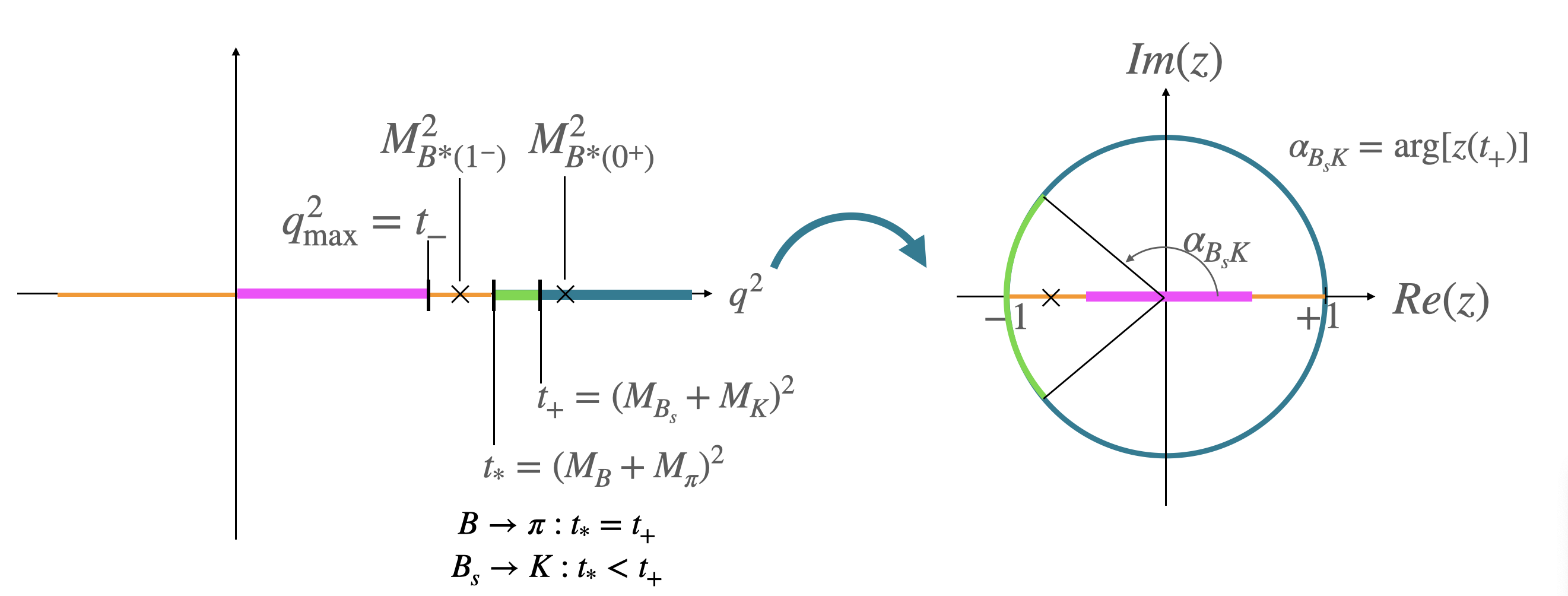
Figure 1: Illustration of the mapping $q^{2}\to z(q^{2})$, showing the physical semileptonic region (magenta), poles (crosses) and branch cuts (light and dark green).

In Fig. 1 we illustrate how the real $q^{2}$ axis maps onto the complex unit disk where the $z$ parameter in Eq. (1) is defined. The physical semileptonic region is mapped to a range on the real $z$ axis around zero, and the branch cut is mapped onto the unit circle. For the $b\to u$ transition in $B\to\pi\ell\nu$ and $B_{s}\to K\ell\nu$ there are two qualitatively different situations: for $B\to\pi\ell\nu$ the relevant two-particle production threshold and lower limit of integration for the corresponding unitarity constraint is at $q^{2}=(M_{B}+M_{\pi})^{2}$, while the relevant threshold for $B_{s}\to K\ell\nu$ is at $(M_{B_{s}}+M_{K})^{2}$, which is the part corresponding to the arc $[-\alpha_{B_{s}K},+\alpha_{B_{s}K}]$ in the $z$-plane, as indicated in the figure (see also [7, 8, 9]). As a result, the corresponding unitarity constraints are

$$\frac{1}{2\pi i}\oint_{C}\frac{dz}{z}\theta_{z}|B_{X}(q^{2})\phi_{X}(q^{2},t_{0})f_{X}(q^{2})|^{2}\leq 1\,,$$ (2)

where the step function $\theta_{z}=\theta(\alpha_{B_{s}K}-|{\rm arg}[z]|)$ in the $B_{s}\to K$ case restricts the integration over the unit circle to the relevant segment, i.e. the one corresponding to the branch cut above the $B_{s}K$ threshold $t_{+}$. Inserting the BGL expansion Eq. (1), the unitarity constraint takes the compact form [1]

$$\sum\limits_{i,j\geq 0}a_{X,i}^{\ast}\langle z^{i}|z^{j}\rangle_{\alpha_{B_{s}K}}a_{X,j}\equiv|{\bf a}_{X}|^{2}_{\alpha_{B_{s}K}}\leq 1\,,$$ (3)

where the inner product is known analytically,

$$\langle z^{i}|z^{j}\rangle_{\alpha}=\frac{1}{2\pi}\int\limits_{-\alpha}^{\alpha}d\phi(z^{i})^{\ast}z^{j}|_{z=e^{i\phi}}=\begin{cases}\displaystyle\frac{\sin(\alpha(i-j))}{\pi(i-j)}&i\neq j\,,\\ \displaystyle\frac{\alpha}{\pi}&i=j\,.\end{cases}$$ (4)

4 Frequentist fit

We begin with the discussion of fits to lattice results for the $B_{s}\to\ K\ell\nu$ scalar $(f_{0}(q_{i}^{2}))$ and vector $(f_{+}(q_{i}^{2}))$ form factors, where we assume that we have data for $N_{0}$ and $N_{+}$ data points respectively. We collect all results in the data vector

$${\bf f}^{\,T}=({\bf f}_{+}^{T},{\bf f}_{0}^{T})=(f_{+}(q^{2}_{0}),f_{+}(q^{2}_{1}),\dots,f_{+}(q^{2}_{N_{+}-1}),f_{0}(q^{2}_{0}),f_{0}(q^{2}_{1}),\dots,f_{0}(q^{2}_{N_{0}-1}))\,.$$ (5)

Correspondingly, we collect the BGL parameters into the parameter vector

$${\bf a}^{T}=({\bf a}_{+}^{T},{\bf a}_{0}^{T})=(a_{+,0},a_{+,1},a_{+,2},...,a_{+,K_{+}-1},a_{0,1},...,a_{0,K_{0}-1})\,.$$ (6)

With this notation the Frequentist fit is defined as the minimisation of

$$\chi^{2}({\bf a},{\bf f})=\left[{\bf f}-Z{\bf a}\right]^{T}C_{\bf f}^{-1}\left[{\bf f}-Z{\bf a}\right]\,,$$ (7)

with respect to the parameters, where $C_{\bf f}$ is the correlation matrix of the input data ${\bf f}$. Details on how the kinematical constraint $f_{+}(0)=f_{0}(0)$ can be implemented through the matrix $Z_{XX}$ can be found in Ref. [1]. Note that we chose to use this constraint to eliminate the parameter $a_{0,0}$, which is therefore missing from the definition of ${\bf a}$ in Eq. (6). The solution for the Frequentist fit is

$${\bf a}=\left(Z^{T}C_{\bf f}^{-1}Z\right)^{-1}ZC_{\bf f}^{-1}{\bf f}\,,\qquad C_{\bf a}=\left(Z^{T}C_{\bf f}^{-1}Z\right)^{-1}\,,$$ (8)

where $C_{\bf a}$ is the covariance matrix of the fit parameters ${\bf a}$.

5 Bayesian fit

Within the Bayesian framework the fit is defined in terms of the expectation value

$$\langle g({\bf a})\rangle=\mathcal{N}\int d{\bf a}\,g({\bf a})\,\pi({\bf a}|{\bf f},C_{\bf f})\,\pi_{\bf a}\,,$$ (9)

where $g({\bf a})$ is a function defined in terms of the BGL parameters. The probability density for the integral is given as

$$\pi_{\bf a}({\bf a}|{\bf f},C_{{\bf f}_{p}})\pi_{\bf a}\propto{\rm exp}\left(-\frac{1}{2}\chi^{2}({\bf a},{\bf f}_{p})\right)\theta(1-|{\bf a}_{+}|_{\alpha}^{2})\theta(1-|{\bf a}_{0}|_{\alpha}^{2})\,,$$ (10)

where the two Heaviside functions restrict the integration to parameters compatible with the unitarity constraint. In Ref. [1] we explain how to estimate the integral in Eq. (9) by means of sampling from a multivariate normal distribution.

6 Results for $B_{s}\to K\ell\nu$

Table 1 shows, as an example, the results for Frequentist fits to the HPQCD 14 data of [10]. The first two columns indicate the order of the fit in a given row for the vector and scalar form factor, respectively. Acceptable fits (see $p$-values in the 3rd-last column) are achieved only for $K_{+}\geq 3$ and $K_{0}\geq 2$. Based on the results in this table, which shows various possible fits with $N_{\rm dof}\geq 1$, solid conclusions about convergence cannot be drawn. Tab. 2 shows the results of the Bayesian fit with $K_{+,0}\leq 8$, where the convergence of the fit parameters is clearly visible. The higher-order coefficients are constrained by the unitarity constraint, which acts as regulator – without this the parameters would not be well constrained.

$K_{+}$	$K_{0}$	$a_{0,0}$	$a_{0,1}$	$a_{0,2}$	$a_{+,0}$	$a_{+,1}$	$a_{+,2}$	$p$	$\chi^{2}_{\rm red}$	$N_{\rm dof}$
2	2	0.0883(44)	-0.250(17)	-	0.0270(13)	-0.0792(50)	-	0.03	2.93	3
2	3	0.0880(44)	-0.242(19)	0.053(65)	0.0273(13)	-0.0760(63)	-	0.02	4.06	2
3	2	0.0906(45)	-0.240(17)	-	0.0257(14)	-0.0805(50)	0.068(31)	0.15	1.89	2
3	3	0.0908(46)	-0.215(22)	0.138(71)	0.0262(14)	-0.0727(64)	0.096(34)	0.97	0.00	1

Table 1: Frequentist fit results for HPQCD 14 data, where $\chi^{2}_{\rm red}=\chi^{2}/N_{\rm dof}$.

$K_{+}$	$K_{0}$	$a_{0,0}$	$a_{0,1}$	$a_{0,2}$	$a_{0,3}$	$a_{0,4}$	$a_{0,5}$	$a_{0,6}$	$a_{0,7}$
2	2	0.0883(44)	-0.250(17)	-	-	-	-	-	-
2	3	0.0880(44)	-0.243(19)	0.052(65)	-	-	-	-	-
3	2	0.0907(46)	-0.240(17)	-	-	-	-	-	-
3	3	0.0906(44)	-0.215(22)	0.137(73)	-	-	-	-	-
3	4	0.0907(47)	-0.215(22)	0.14(11)	-0.01(31)	-	-	-	-
4	3	0.0907(45)	-0.214(22)	0.139(72)	-	-	-	-	-
4	4	0.0907(46)	-0.215(25)	0.12(19)	-0.08(60)	-	-	-	-
5	5	0.0909(46)	-0.218(25)	0.10(19)	-0.12(55)	0.04(63)	-	-	-
6	6	0.0907(45)	-0.217(25)	0.10(19)	-0.11(53)	0.06(66)	-0.02(66)	-	-
7	7	0.0907(46)	-0.217(26)	0.11(20)	-0.08(51)	0.03(73)	0.03(81)	-0.04(70)	-
8	8	0.0908(46)	-0.217(25)	0.11(20)	-0.08(50)	-0.01(84)	0.1(1.0)	-0.09(96)	0.08(74)

Table 2: Results for BGL coefficients for the scalar form factor (results for the vector form factor can be found in [1]).

While the Frequentist fit can provide important information about the compatibility of the fit function with the data, the Bayesian fit allows for a meaningful imposition of the unitarity constraint and also to study the convergence of the BGL parameterisation. We think that future analyses of form-factor data should take advantage of this complementarity.

7 $B\to D^{\ast}\ell\nu$ fit

The method can be extended to other decay channels such as the semileptonic decay of a pseudo-scalar to a vector particle. We consider the case of $B\to D^{\ast}\ell\nu$ for which lattice data exists from FNAL/MILC [11], HPQCD [12] and JLQCD [13].

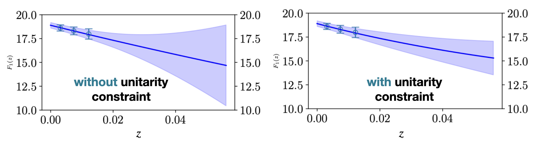
Figure 2: Result for BGL fit to JLQCD data [13] for the $B\to D^{\ast}\ell\nu$ form factor $\mathcal{F}_{1}$. Fit without (left) and with (right) unitarity constraint.

Fig. 2 shows the result for the form factor $\mathcal{F}_{1}$ from a simultaneous fit to the JLQCD data over all four form factors $f,\,g,\,\mathcal{F}_{1},\,\mathcal{F}_{2}$, including kinematical constraints between $\mathcal{F}_{1}$ and $f$, and $\mathcal{F}_{1}$ and $\mathcal{F}_{2}$, respectively. The plots show the fit results once without imposing unitarity and once with. The result of imposing unitarity is a substantial reduction in the statistical error in the extrapolation of the lattice data towards zero momentum transfer (towards the right-hand side of the plots).

8 Conclusions

We presented novel ideas for fitting model- and truncation-independent parametersations to data for semileptonic decay form factors. The combination of information from Frequentist and Bayesian fits allows for a comprehensive understanding of fit-quality and truncation dependence. Moreover, the Bayesian framework allows for a meaningful imposition of the unitarity constraint to regulate the determination of fit parameters and, as demonstrated for the case of $B\to D^{\ast}\ell\nu$, to reduce the statistical error in form-factor extrapolations. The code underlying the results of [1] is publicly available under [14].

References

- [1] J. M. Flynn, A. Jüttner, and J. T. Tsang, Bayesian inference for form-factor fits regulated by unitarity and analyticity, arXiv:2303.11285.
- [2] J. T. Tsang and M. Della Morte, B-physics from Lattice Gauge Theory, arXiv:2310.02705.
- [3] RBC/UKQCD Collaboration, J. M. Flynn, R. C. Hill, A. Jüttner, A. Soni, J. T. Tsang, and O. Witzel, Exclusive semileptonic →K decays on the lattice, Phys. Rev. D 107 (2023), no. 11 114512, [arXiv:2303.11280].
- [4] C. G. Boyd, B. Grinstein, and R. F. Lebed, Constraints on form-factors for exclusive semileptonic heavy to light meson decays, Phys. Rev. Lett. 74 (1995) 4603–4606, [hep-ph/9412324].
- [5] I. Caprini, L. Lellouch, and M. Neubert, Dispersive bounds on the shape of form-factors, Nucl. Phys. B530 (1998) 153–181, [hep-ph/9712417].
- [6] C. Bourrely, I. Caprini, and L. Lellouch, Model-independent description of decays and a determination of , Phys. Rev. D79 (2009) 013008, [arXiv:0807.2722]. erratum: Phys. Rev. D82 (2010) 099902.
- [7] N. Gubernari, D. van Dyk, and J. Virto, Non-local matrix elements in , JHEP 02 (2021) 088, [arXiv:2011.09813].
- [8] N. Gubernari, M. Reboud, D. van Dyk, and J. Virto, Improved theory predictions and global analysis of exclusive processes, JHEP 09 (2022) 133, [arXiv:2206.03797].
- [9] T. Blake, S. Meinel, M. Rahimi, and D. van Dyk, Dispersive bounds for local form factors in transitions, arXiv:2205.06041.
- [10] C. Bouchard, G. P. Lepage, C. Monahan, H. Na, and J. Shigemitsu, form factors from lattice QCD, Phys.Rev. D90 (2014), no. 5 054506, [arXiv:1406.2279].
- [11] Fermilab Lattice, MILC, Fermilab Lattice, MILC Collaboration, A. Bazavov et al., Semileptonic form factors for at nonzero recoil from -flavor lattice QCD: Fermilab Lattice and MILC Collaborations, Eur. Phys. J. C 82 (2022), no. 12 1141, [arXiv:2105.14019]. [Erratum: Eur.Phys.J.C 83, 21 (2023)].
- [12] J. Harrison and C. T. H. Davies, vector, axial-vector and tensor form factors for the full range from lattice QCD, arXiv:2304.03137.
- [13] JLQCD Collaboration, Y. Aoki, B. Colquhoun, H. Fukaya, S. Hashimoto, T. Kaneko, R. Kellermann, J. Koponen, and E. Kou, semileptonic form factors from lattice QCD with Möbius domain-wall quarks, arXiv:2306.05657.
- [14] A. Jüttner, BFF – Bayesian Form factor Fit code https://github.com/andreasjuettner/BFF, https://doi.org/10.5281/zenodo.7799543, .