Timing Performance of the CMS High Granularity Calorimeter Prototype

Abstract

This paper describes the experience with the calibration, reconstruction and evaluation of the timing capabilities of the CMS HGCAL prototype in the beam tests in 2018. The calibration procedure includes multiple steps and corrections ranging from tens of nanoseconds to a few hundred picoseconds. The timing performance is studied using signals from positron beam particles with energies between 20 GeV and 300 GeV. The performance is studied as a function of particle energy against an external timing reference as well as standalone by comparing the two different halves of the prototype. The timing resolution is found to be 60 for single-channel measurements and better than 20 for full showers at the highest energies, setting excellent perspectives for the HGCAL calorimeter performance at the HL-LHC.

1 Introduction

In recent years there has been a growing interest in precision timing for uses beyond the traditional time-of-flight measurements for particle identification. In anticipation of the very large number of simultaneous interactions that will occur in a single bunch crossing (pile up) at the High-Luminosity LHC (HL-LHC), both the CMS and ATLAS Collaborations are developing specialized detectors that can measure the time of the passage of a charged particle with a precision of a few 10. These detectors will allow the separation of different proton-proton interactions within a single bunch crossing, which occurs over an interval of about 350.

As part of the detector upgrade for the HL-LHC, the CMS Collaboration will replace the two endcap calorimeters with new, high-granularity, sampling calorimeters (HGCAL, or CE for Calorimeter Endcap). The electromagnetic sections of HGCAL will be instrumented entirely with silicon sensors, while the hadronic sections will be equipped with silicon sensors in the regions of the calorimeter where the total fluence is expected to be above 5e13$\mathrm{n_{eq}}/\mathrm{cm}^{2}$, and with plastic scintillators read out by silicon photomultipliers (SiPMs) elsewhere. Full details of the CMS endcap calorimeter upgrade may be found in Ref. [1].

In the development program for the HGCAL, a series of tests with single components and prototypes of the calorimeter have been conducted using early versions of the readout electronics [2]. We report here on the results obtained on the time development of electromagnetic showers based on data collected with a prototype calorimeter in the H2 beam line of the CERN Super Proton Synchrotron (SPS) in 2018. Although the prototype did not fully represent the final detector and electronics components, it allowed the main performance features of the final system to be studied. In 2016, in a beam test with single prototype silicon diode sensors at the SPS the intrinsic timing resolution of the silicon sensors was evaluated [2]. In the beam test reported here, the timing performance of a 28-layer electromagnetic calorimeter with a full analog read-out chain with precision timing in each channel was measured.

Previous publications have described the construction and the data acquisition system of this prototype calorimeter [3, 4], and the energy resolution, linearity, and position and angular resolutions for both positrons and charged pions [5, 6].

2 Experimental setup

2.1 Infrastructure at the SPS H2 beam line

Data were collected in October 2018 at the H2 beamline [7] at the CERN-SPS North Area. Full details of the beamline may be found in Ref. [5]. This study used a secondary beam of positrons with a momentum of up to 300 GeV/c.

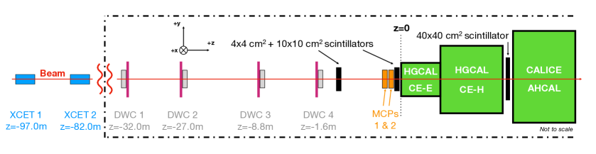
Figure 1: The HGCAL prototype experimental setup used during the 2018 test beam. The electromagnetic section, which is the focus of this paper, is denoted as CE-E. It is preceded (to the left) by multiple ancillary beam instrumentation detectors, and is followed by detector prototypes dedicated to the study of hadron showers.

The experimental setup is sketched in Figure 1. Two micro-channel plate (MCP) detectors [8] were placed immediately upstream of the CE-E prototype to provide a reference measurement of the time-of-arrival of the incident particles. The sensitive area of the MCP detectors was about 1 cm , defining the transverse extent of the accepted events. One of the MCP detectors (MCP 1) was used as a timing reference, while the second one was used for cross-calibration to obtain the timing resolution as a function of the signal amplitude, shown in Figure 2. The MCP timing resolution depends on the deposited charge and the asymptotic timing resolution of a single MCP was found to be about 9. The average resolution for positrons selected for this study was measured to be about 25 corresponding to MCP signals of about 700ADC counts.

Figure 2: Single MCP time resolution estimated as $\sigma/\sqrt{2}$, where $\sigma$ comes from a Gaussian fit to the distribution of time differences between the two MCPs operated in front of the HGCAL prototype calorimeter. Given the identical structure of the two MCP detectors, their timing resolution was assumed to be identical.

Two scintillators, used to generate the event trigger, were placed before and after the MCP detectors. Four delay wire chambers used to determine the impact position of beam particles were placed upstream of the trigger scintillators. Further details of the experimental setup can be found in Ref. [5].

2.2 2018 HGCAL prototype

Full details of the detector construction and its readout electronics can be found in Refs. [3, 4]. In summary, the calorimeter prototype comprised three sections shown in Figure 1: the silicon electromagnetic calorimeter (CE-E), the silicon hadronic calorimeter (CE-H), and the tile hadronic calorimeter (AHCAL). The electromagnetic calorimeter was constructed with $28$ hexagonal detector modules, each of which was assembled as a glued stack, consisting of a sintered copper-tungsten baseplate, a silicon sensor, and a printed circuit board with the front-end readout electronics. The hexagonal silicon sensor was sub-divided into 128 hexagonal pads, each with a surface of about 1.1 cm . To bias the sensor and shield it from electromagnetic interference, two metalized polyimide layers were used between the sensor and the base plate. The $28$ modules in the electromagnetic calorimeter were mounted in pairs on either side of copper cooling plates and these were interleaved with lead absorber plates. The first $26$ layers of the electromagnetic section featured 300 thick sensors, while the last two used 200 thick sensors. The CE-E was approximately 50 cm long totaling about $28$ radiation lengths, to ensure sufficient longitudinal containment of electromagnetic showers.

2.2.1 Time measurement with the SKIROC2-CMS ASIC

A 64-channel front-end readout ASIC was used to read out the modules. The ASIC, SKIROC2-CMS, was developed specifically for these tests by the OMEGA microelectronics group [9]. The overall ASIC architecture and the data and control handling are described in detail in Refs. [3, 4]. The ASIC measured both the amplitude and the time of arrival of the signals in each of the 64 channels. The signal amplitude was measured with two preamplifiers, with high and low gains, and a shaping time of 40, whose outputs were digitized with separate Wilkinson ADCs. For the largest amplitude signals, a time-over-threshold (TOT) circuit was used.

The signal time was determined using a time-of-arrival (TOA) measurement relative to a common 40 MHz system clock. The output of the preamplifier was fed into a fast shaper, with a shaping time of 5, to remove high-frequency noise, and to shape the signal for input to a constant-threshold discriminator. The shaping time was chosen for optimal noise performance and to minimize time-walk effects, and the discriminator threshold was set to an energy corresponding to approximately 15, where 1 corresponds to the average energy deposited by a minimum ionizing particle in the silicon sensor. The output of the discriminator triggered two separate time-to-amplitude converter (TAC) circuits each with a voltage ramp, one of which was stopped on the subsequent rising edge of the clock, and the other on the falling edge, as illustrated in Figure 3. The first clock edge was skipped to avoid the strong non-linearity at the start of the voltage ramps. When the ramps were stopped, the voltage levels were stored in an analog memory and later digitized with a 12-bit Wilkinson ADC, similar to the one used in the gain measurements. Due to the operation mode of the TACs, targeting the best possible time resolution of about 50, the time measurement became non-linear for the last 12. This was compensated by combining the rising and falling edge measurements, as described in Section 3.

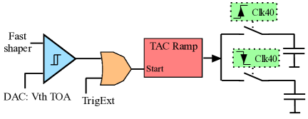
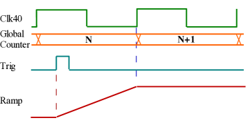
Figure 3: Block diagram of the SKIROC2-CMS time-of-arrival (TOA) analog circuit (left) and an illustration of the time-to-amplitude converter (TAC) ramp (right) that is stopped by a clock edge. An external trigger signal can be used to perform characterization and calibration of the TAC circuitry. Reproduced from Ref. [10].

2.2.2 Clock path in the DAQ system

The 40 system clock was generated with an oven-controlled quartz crystal oscillator (OCXO) on a custom-designed synchronization board (SB), which distributed the clock via HDMI cables to 14 custom-designed readout boards (RB). These, in turn, distributed the clock to seven detector modules via interposer boards, as shown in Figure 4. The overall architecture is described in Ref. [3]. A copy of the 40 clock was also sent via an RG157 cable to a CAEN v1742 digitizer, which was also used to read out the analog signals from the two MCP detectors.

The jitter of the clock distribution system, from the clock-generating SB to the RBs, was measured in laboratory to be less than 10. However, the jitter of the clock between SB and the CAEN v1742 could not be determined in laboratory tests and was estimated to be $50\text{\,}\mathrm{ps}$ from in situ measurements, as discussed below in Section 4.1.

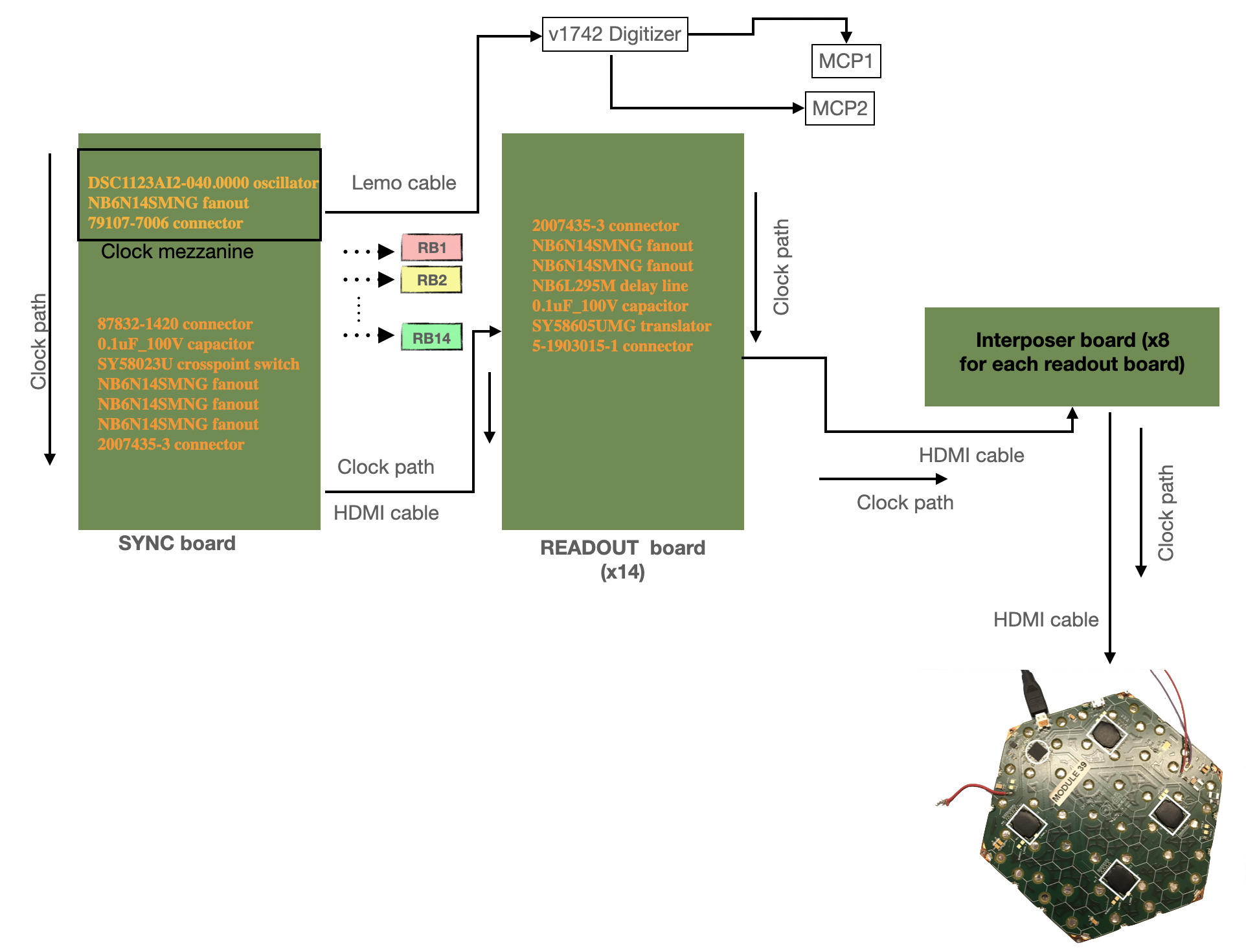
Figure 4: Schematic view of the clock distribution tree in the experimental setup. All components on the clock path are explicitly mentioned. Laboratory measurements of the jitter from the synchronization board to the readout board outputs was measured to be less than 10 as expected.

2.3 Datasets

Data were collected with the HGCAL prototype with beams of positrons with energies between 20 GeV and 300 GeV, with approximately $50\,000$ events collected at twelve different energies.

A Geant4 [11] model of the experimental setup, including ancillary devices in the beam line, was used to simulate the detector response. This model is the same one used in Ref. [5], where it is described in detail.

In order to obtain a realistic time resolution in the simulation, the time of the signal was convoluted with a Gaussian that had a width determined empirically for each channel. Still, the model does not include the response of electronics components or the digitization, and thus any response non-linearities or similar effects are not simulated.

3 Reconstruction of the timing information

The sequence of the time measurement in the ASIC is shown schematically in Figure 5. When the signal goes above a fixed threshold, the TAC ramps are started, and after skipping the first clock edge, the ramps are stopped: one on the rising edge of the clock, and the second one on the falling edge of the clock. This yields two time measurements, TOA-rise and TOA-fall, from which two separate signal times are estimated, $T_{\text{rise}}$ and $T_{\text{fall}}$. These times are referenced to the system clock after corrections for the non-linearity of the TAC ramp, the time-walk that depends on the hit energy, and the deposited energy in the full module.

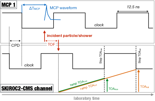
Figure 5: Timing measurements used in the calibration of the calorimeter hit timestamps. $CPD$ denotes an arbitrary but constant clock-phase-difference between a given readout channel and the reference clock. TOF refers to the time-of-flight between the MCP and silicon sensor.

3.1 Signal time reconstruction

To estimate the signal time, $T$, the procedure for both TOA measurements was as follows:

1. The measured TOA values were normalized to the unit interval to take into account their pedestal values,

2. the TOAs were corrected for the non-linearity of the TAC ramp ($f_{\text{TOA}}$),

3. an amplitude-dependent time walk correction ($f_{\text{TW}}$) was applied, and

4. a correction for small signals ($f_{\text{R}}$) that depends on the total energy deposited in the module containing the channel ($E_{\text{module}}$) was applied.

It is worth noting that the first two steps operate on TOA values and their distribution, whereas the last two steps operate on individual signal times. Accordingly, the signal time, $T$, for each channel has three contributions, as shown in Equation 3.1:

$$T_{\text{rise/fall}}~{}=~{}f_{\text{TOA}}(TOA_{\text{rise/fall}})~{}+~{}f_{\text{TW}}(E_{\text{hit}})~{}+~{}f_{\text{R}}(E_{\text{module}},E_{\text{hit}}).$$ (3.1)

The signal time $T$ in any given channel is estimated separately from both TOA-rise and TOA-fall.

3.2 Derivation of the corrected time

As the beam particles were asynchronous with respect to the 40 system clock, the signal arrival times were uniformly distributed within the 25 clock period. This resulted in the full range of possible TOA values being available for the determination of the non-linearity corrections.

The signal from MCP1 was required to have an amplitude greater than 500ADC counts, where the time resolution was better than 40, as shown in Figure 2. Also, only readout channels with more than $1000$ hits with $E_{\text{dep}}\geq\qty{250}{}$ and with $30\,000$ or more hits in total were considered. The first requirement selects a large sample of measurements where the energy is estimated from the TOT measurement, i.e. not from the ADC measurement. As the beam was focused on the center of the calorimeter, only $116$ readout channels, or 3% of all channels, met these requirements.

3.2.1 Correction of the non-linearity of the TOA

First, variations in pedestals ($TOA^{\text{min}}$) were corrected, and the values were scaled by the full range ($\Delta TOA$), yielding $TOA_{\text{norm}}$ normalized to unity, thus corresponding to the relative location of the TOA value in the clock period:

$$TOA_{\text{norm}}~{}\coloneqq~{}\frac{TOA-TOA^{\text{min}}}{\Delta TOA}.$$ (3.2)

After this normalization, the non-linear response of $TOA_{\text{norm}}$ was corrected using the MCP measurement, which was considered linear. For each channel the response was modelled using

$${f}_{TOA}(TOA_{\text{norm}}|\vec{\Theta})~{}=~{}\Theta_{1}\cdot x+\Theta_{2}+\frac{\Theta_{3}}{x-\Theta_{4}},$$ (3.3)

where $\vec{\Theta}$ is a set of parameters describing the response of the TOA measurement.

The accuracy of this response linearization is improved by using separate $\vec{\Theta}$ parameter sets in the linear ($TOA_{\text{norm}}<0.65$) and non-linear regions ($TOA_{\text{norm}}\geq 0.65$).

The result of the linearization step is shown in Figure 6(a) for the normalized TOA-rise of a representative channel, where the full 25 range is presented. This method is found to be in agreement with the previous response correction presented in Ref. [10], that did not rely on the MCP reference but on the asynchronous nature of the beam particles.

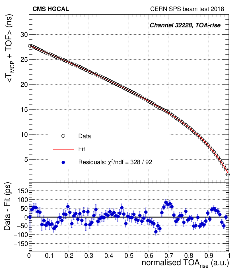
(a) TOA linearization, Section 3.2.1.

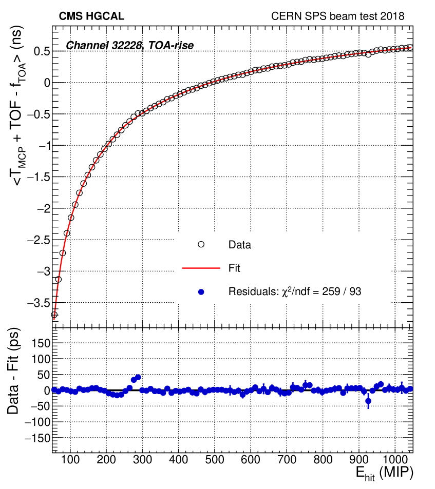
(b) Time-walk correction, Section 3.2.2.

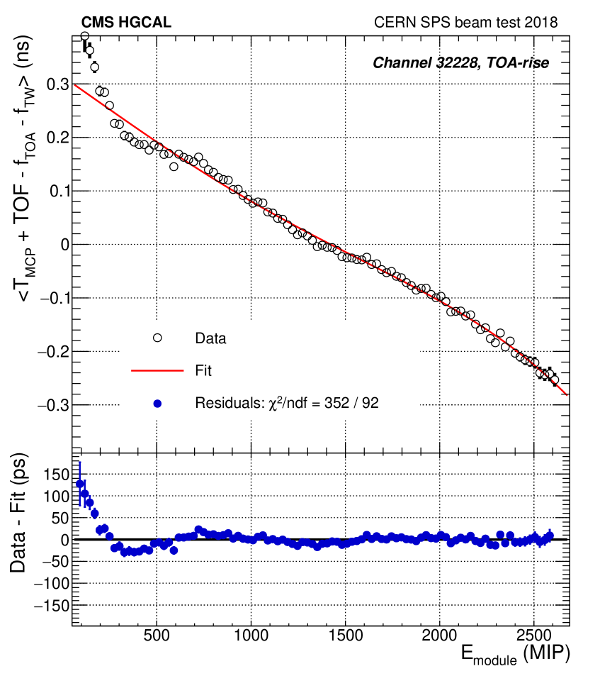
(c) Residual correction, Section 3.2.3.

Figure 6: The three TOA calibration steps (TOA-rise in this case) of a representative channel, centrally located inside the HGCAL prototype: (a) Linearization of the normalized TOA, (b) assessment of the signal-induced time-walk correction, and (c) assessment of the residual correction, a smaller time-walk that depends on the total energy in the module of the given channel. The magnitude of the time-walk corrections is about one and two orders of magnitude smaller than the calibrated time range, respectively. The additive TOF term represents the constant time offset between the MCP and the readout channel.

3.2.2 Time-walk correction

The $f_{\text{TOA}}$ linearization corrections were followed by an amplitude-dependent correction for the time-walk effect. This correction is derived from a fit to the TOA time difference to the MCP as a function of the reconstructed signal amplitude, $E_{\text{hit}}$ using the same functional form as in Equation 3.3. It was also found that the fit was improved by separately fitting two regions of the signal amplitude depending on whether the ADC ($E_{\text{hit}}<E_{\text{TOT}}$) or the TOT is used ($E_{\text{hit}}\geq E_{\text{TOT}}$) to estimate the hit energy:

$$f_{\text{TW}}(E_{\text{hit}})~{}\coloneqq~{}\begin{cases}{f}_{TOA}(E_{\text{hit}}|\vec{\Theta}_{1}^{TW})&\text{for }E_{\text{hit}}<E_{\text{TOT}}.\\ {f}_{TOA}(E_{\text{hit}}|\vec{\Theta}_{2}^{TW})&\text{for }E_{\text{hit}}\geq E_{\text{TOT}}.\end{cases}$$ (3.4)

The value of $E_{\text{TOT}}$ was determined channel-by-channel and is typically a few hundred MIPs [4]. As can be seen in Figure 6(b), the time-walk is found to reach several nanoseconds for hit energies below a few 100.

3.2.3 Residual time-walk correction depending on module energy

After the linearization and time-walk corrections, timing corrections of the order of a few 100 were needed for small energies. This effect depended on the total energy deposited in the module that channel belonged to, $E_{\text{module}}$. It is likely that this effect is due to the common-mode estimation procedure [4] that is applied only to small signals measured with the ADC signals and not to large ones measured with the TOT. We found that this residual correction can be well modeled by

$$f_{\text{R}}(E_{\text{module}},E_{\text{hit}})~{}\coloneqq~{}\begin{cases}\mathcal{P}_{4}(E_{\text{module}})&\text{for }E_{\text{hit}}<E_{\text{TOT}},\\ 0&\text{for }E_{\text{hit}}\geq E_{\text{TOT}},\end{cases}$$ (3.5)

where $\mathcal{P}_{4}$ represents a fourth-degree polynomial whose parameters are determined from a fit to the average of the reference timestamps corrected by $f_{\text{TOA}}+f_{\text{TW}}$, as a function of $E_{\text{module}}$. Figure 6(c) shows the residual correction determined for a representative channel.

3.2.4 Combination of TOA-rise and TOA-fall

If both TOA-rise and TOA-fall values are within their linear region, the time is computed from the average of the two timing estimates. Otherwise, the variant in, or closest to, its linear region is retained.

After all corrections were applied the estimated precision of the time measurement among the 116 channels for which the time calibration procedure was possible is about 50.

The fitted calibration parameter values for the example channel illustrated in Figure 6 are provided in Appendix A. The parameter values vary by about 10% over the calibrated channels. The analysis of the timing performance of the detector discussed below is restricted to those channels, that are located centrally in the prototype.

To illustrate the results of the timing reconstruction and calibration procedure, Figures 7(a), 7(b) and 7(c) show the time evolution of the hits from a 250 GeV positron showering in the calorimeter. A subset of the calibrated channels is visible along the core of the shower, and a clear correlation is observed between the reconstructed time and the spatial development of the shower, as expected. For this event, the reconstructed hit energies vary by a factor of about 20.

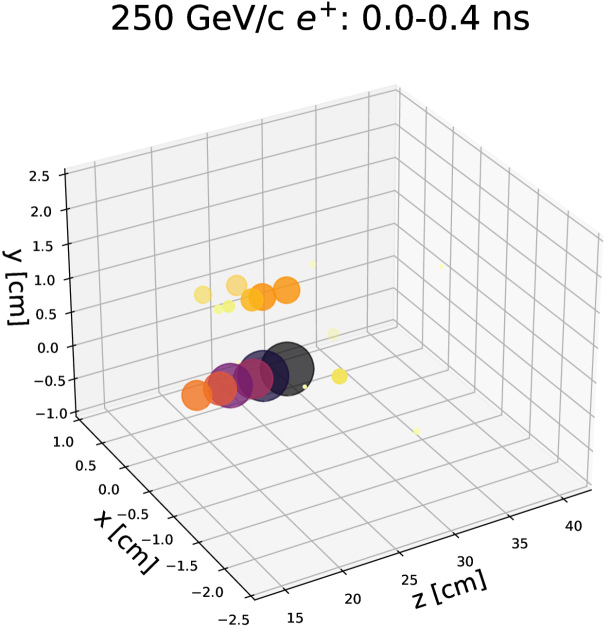
(a) $\qty{0}{}\leq T\leq\qty{0.4}{}$.

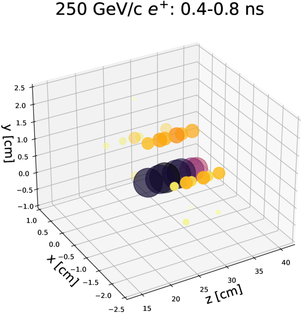
(b) $\qty{0.4}{}<T\leq\qty{0.8}{}$.

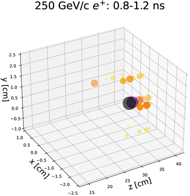
(c) $\qty{0.8}{}<T\leq\qty{1.2}{}$.

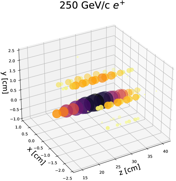
(d) Full shower.

Figure 7: Time evolution (a–c) of a shower (d) induced by a 250 GeV positron in the HGCAL prototype. Data are shown for $81$ hits with reconstructed timestamps in this event. Hit energies are proportional to larger and darker markers, and are provided solely for illustration purposes.

4 Timing performance of single channels and full showers in the HGCAL prototype

In this section we describe the time performance from the single channel level to full showers in the prototype. First, the time resolution is determined for individual channels using the MCPs as an external reference. Then, this resolution model is injected into the simulation and compared to the shower timing as measured in the particle data. Further studies of the HGCAL-only full shower time resolution conclude this section.

4.1 Single channel performance

The per-cell timing performance is a fundamental ingredient to build a realistic simulation with which one can gauge the shower timing measurements obtained in data.

The average per-cell timing performance of the calibrated TOA values is quantified as a function of the corresponding energy deposit. For this purpose, the TOA values are compared to a reference time measurement in bins of energy, and fitted using a Gaussian resolution function. The measured average time is found to be rather flat as a function of the energy, with deviations up to about 20 in the very low energy region (below 300), that are consistent with the outcome of the calibration procedure described in Section 3. The measured resolution as a function of the deposited energy is shown in Figure 8 for two different choices of reference time measurement: in Figure 8(a) (black) the reference time is provided by the MCP system, while in Figure 8(b) it is provided by one silicon cell within the HGCAL. In Figure 8(b), results are shown for pairs of cells from different modules (orange) and in the same module and different ASICs (blue). The measurements in Figure 8 are fitted with $\sigma^{2}(E)=(a/E)^{2}+c^{2}$, where $E$ represents the energy, $a$ is a constant that represents the improvement in resolution with energy, and $c$ is a constant term.

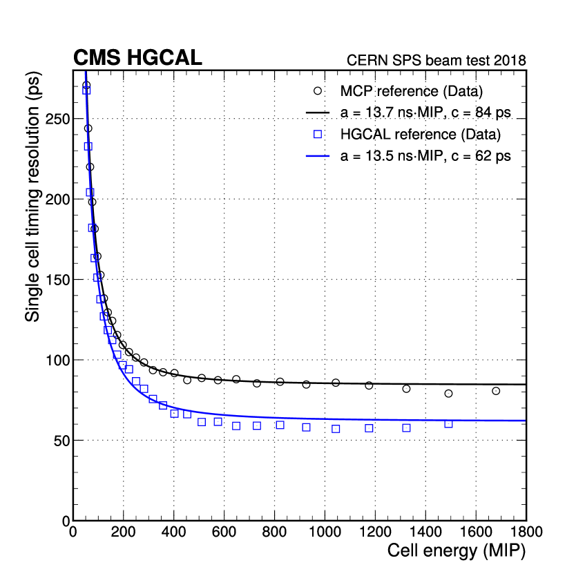
(a) Single-channel timing performance taking the MCP (black circles) or the HGCAL shower measurement (blue squares) as reference.

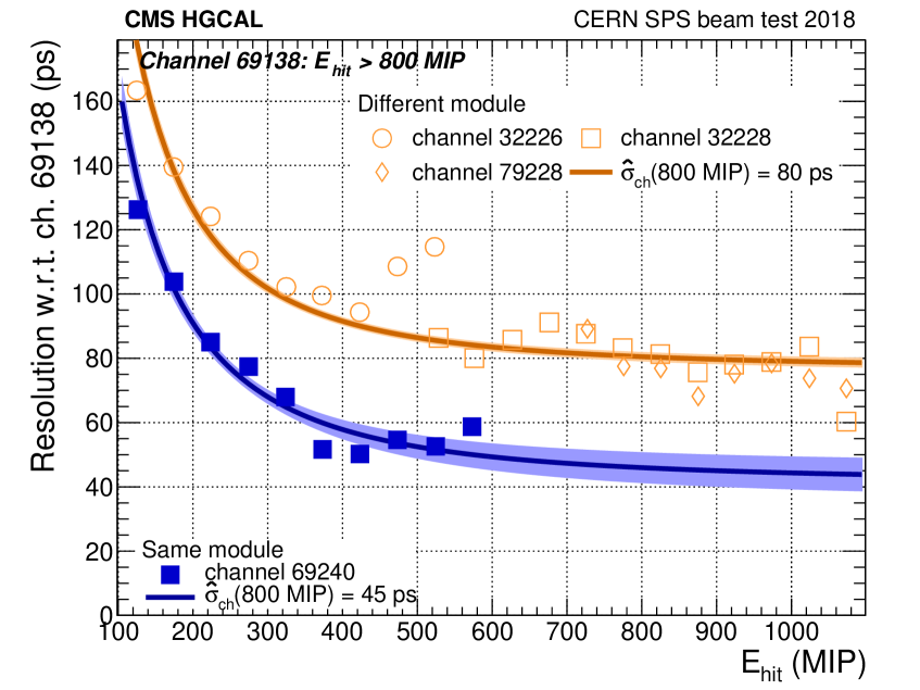
(b) Single-channel timing performance taking as the reference a different silicon channel from a different module (orange, open) or from a different ASIC on the same module (blue, filled).

Figure 8: Single-cell time resolution as a function of the cell energy in data, computed against different timing references: In (a) the MCP measurement or the average time of the shower measured with the HGCAL prototype are used. The difference in performance between the MCP and HGCAL references is evidence of a jitter between the two systems. In (b) a reference silicon channel is used, that is chosen from a different module or from a different ASIC of the same module. The difference in performance between the same-module and different-module references is evidence of a correlation between the timing measurements of different channels.

The constant term of the black curve in Figure 8(a) includes the contribution of ∼25 due to the intrinsic timing resolution of the MCP system used as reference (Figure 2), providing a measurement of the average per-cell asymptotic timing resolution of about 80.
In Figure 8(b), the difference between the constant terms determined from the same-module and different-module pairs indicates strong correlations in the timing measurement of different channels within the same module. To estimate this correlation, we fit to the data a model that assumes the same timing resolution for all silicon cells and one single correlation coefficient independent of the cell energy or its position within the module. The fit yields a constant term for uncorrelated cells of about 60 and a correlation coefficient $\rho\sim 0.8$ between the timing measurements of cells in the same module. This correlation was found to have a negligible impact on the results, as discussed in Appendix B. The difference between the per-cell constant terms when measured with the MCP and a with a silicon cell reference, indicates the presence of an additional smearing of about 50 between the HGCAL prototype and the MCP system. Although the source of this extra jitter could not be identified, we believe that it is constant and random, and thereby does not affect the performance of the calibration procedure of Section 3.

To measure the intrinsic timing performance of the HGCAL prototype, the calibrated TOA values are compared to an internal timing reference provided by the average time of the shower measured with the calorimeter prototype, as described in Section 4.2. Such a quantity is independent of any offset between the HGCAL prototype and the MCP system and is dominated by the per-cell timing resolution. The corresponding result is shown in Figure 8(a) (blue squares) and fitted with the same resolution function. The resulting energy-dependent term is essentially the same as that obtained when using the MCP as the reference, while the difference between the two constant terms is consistent with the intrinsic timing resolution of the MCP system plus the inferred extra global event jitter.

As a summary of Figure 8, the timing resolution representative of the average per-channel performance, measured with the full readout chain, can be expressed as a function of the deposited energy as:

$$\sigma^{2}(\mbox{E})\approx\left(\frac{\qty{13.5}{\cdot}}{\mbox{E}}\right)^{2}+(\qty{62}{})^{2}$$ (4.1)

This resolution agrees with the electronics specifications of the SKIROC2-CMS ASIC and is used for the smearing of the Geant4-simulated hit timestamps for the analysis presented in the following sections.

4.2 Full shower performance

The timing performance measured for full showers in data is compared to the Geant4 simulation introduced in Section 2.3. Realistic timing values are simulated by smearing the TOA values from Geant4 with the average per-cell time resolution as discussed in Section 4.1 and given in Equation 4.1, including a term dependent on the energy deposited in the cell that is uncorrelated among the cells, and a constant term of about 60. This constant term includes a contribution from the MCP measurement of 25 and an additional jitter, discussed in Section 4.1, of about 50. Both contributions to the constant term are correlated over all the cells.

The average time of a shower, $\bar{t}$, is estimated as the weighted average over the times, $t_{i}$, of the ($n$) contributing cells:

$$\bar{t}=\frac{\Sigma^{n}_{i=1}{w_{i}t_{i}}}{\Sigma^{n}_{i=1}{w_{i}}}\mbox{, where }w_{i}=\frac{1}{\sigma^{2}\left(E_{hit}\right)}$$ (4.2)

These shower time values are then fitted with a Gaussian function in bins of the particle beam energy. This allows to extract the average time and its standard deviation as a function of the impinging particle energy. The standard deviation from this fit is referred to in the following as the fitted resolution. For comparison, the average of the per-event uncertainty is also computed, and referred to as expected resolution, $\sigma_{\bar{t}}$, in the following:

$$\sigma_{\bar{t}}=\frac{1}{\sqrt{\Sigma^{n}_{i=1}{w_{i}}}}$$ (4.3)

Figure 9 shows the results for the average shower time and the fitted and expected resolutions, as well as a good agreement between data and simulation, when including all previously-discussed smearing terms. The presence of the additional jitter between the calorimeter prototype and the MCP detectors clearly deteriorates the observed timing resolution performance for full showers. The constant term of about 58 is compatible with the sum in quadrature of the MCP intrinsic resolution of about 25 (Figure 2), the expected calorimeter performance of about 16 (Figure 9(b)), and an additional jitter of about 50.

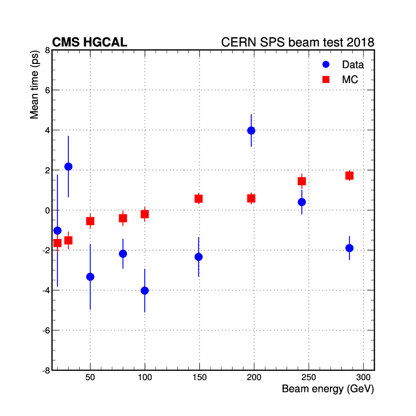
(a) Average shower time showing an accuracy better than 10 across the full range of energies probed.

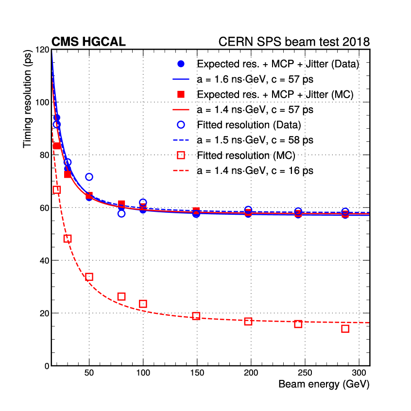
(b) Fitted and expected shower timing resolutions. The fitted resolution in data is dominated by the additional jitter between the calorimeter prototype and the MCP detectors.

Figure 9: For positron showers contained in the HGCAL prototype, their (a) average time and (b) timing resolution as a function of the beam energy, for both beam data and simulated Monte Carlo (MC) data. For beam data, both the fitted and the expected resolutions are shown, as discussed in the text.

4.2.1 Intrinsic timing resolution of the HGCAL prototype

The intrinsic timing performance of the HGCAL prototype can be characterized in spite of the experimental jitter observed between the calorimeter and the MCP devices. This is achieved by splitting the calorimeter into two equivalent halves for analysis purposes, each half acting as a reference and a target timing measurement, respectively. Even and odd layers are considered separately, and the time difference between the two half-showers reconstructed in each of the halves of the calorimeter is taken on an event-by-event basis. The intrinsic time resolution is then determined under the assumption of similar time resolution of both halves, by taking the standard deviation of the time difference between the halves divided by $\sqrt{2}$.

Figure 10 shows the half-shower timing resolution as a function of the beam energy. The estimated value of the energy-dependent term, $a$, is a factor of $\sqrt{2}$ larger than what is found in Figure 9(b), which is consistent with the using half the number of sampling layers. The constant term, on the other hand, is almost twice smaller than when using the MCP as reference, due to the absence of the jitter between the MCP and the HGCAL prototype and the green markers in Figure 10 illustrate the estimated performance when using all layers for the shower timing determination.

The constant term of about 16 for the full calorimeter prototype estimates in Figure 10 is consistent with the constant term for simulated data that does not include the 50 correlated jitter that is shown in Figure 9(b).

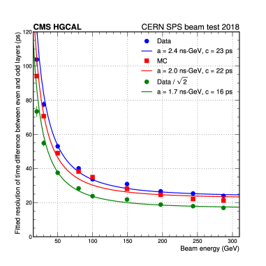
Figure 10: Resolution of the event-by-event difference between the time of positron half-showers computed with only even layers and only odd layers separately, as obtained for beam data (blue) and simulated Monte Carlo (MC) data (red). The green markers correspond to beam data resolutions divided by $\sqrt{2}$, and are an estimate of the performance expected if all the layers were used for the shower time estimation. These measurements are not affected by the jitter between MCP and HGCAL, as discussed in the text.

4.2.2 Timing properties of the shower

Since the timing resolution of a shower depends both on the energy of the hits and on the number of hits, the time resolution is studied as a function of these two quantities. The results for beam data are shown in Figure 11 for reconstructed showers using all layers. The resolution is observed to scale according to the expectation, with a continuous trend across different beam particle energies and hit multiplicities. The smooth trends observed in Figure 11 are all the more relevant when considering the underlying variety of beam conditions, such as the beam profile that changes substantially with the beam energy.

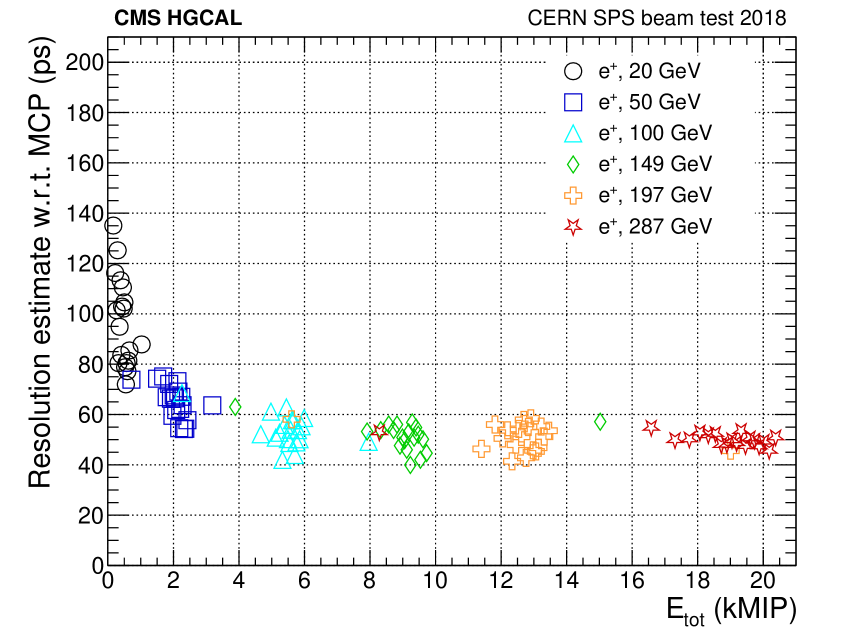
(a)

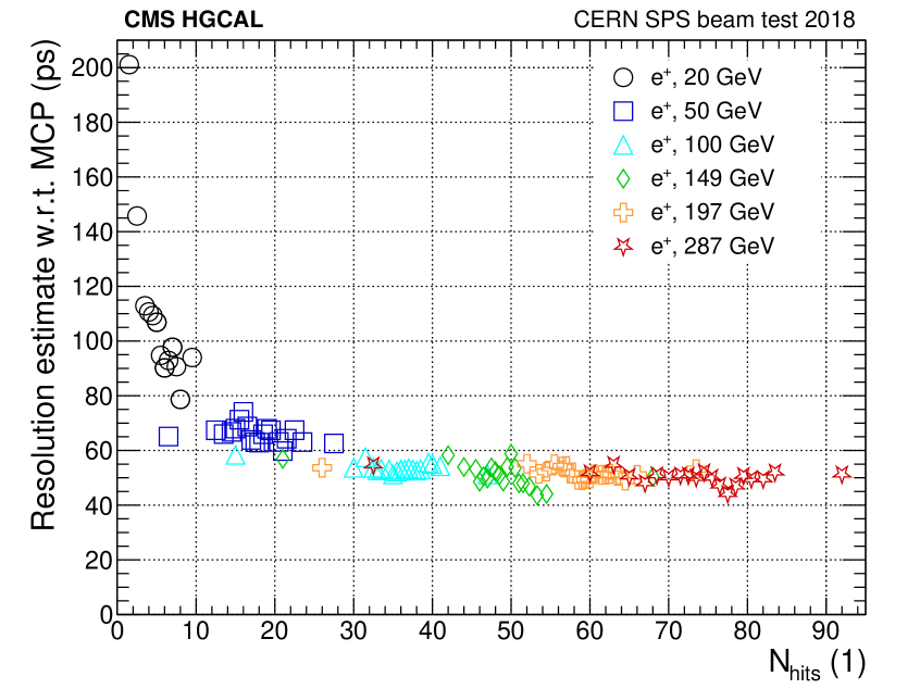
(b)

Figure 11: Time resolution of the reconstructed positron showers as a function of (a) the energy sum and of (b) the number of hits. The smooth variation of the resolution with these two quantities shows that the shower time determination is stable with respect to varying beam conditions, including different beam profiles.

The time distribution of the fraction of hits that were calibrated and used in the reconstruction of 300 GeV positron showers is displayed in Figure 12(a) for both beam data and simulated data, showing a good agreement between the two. For the same showers, Figure 12(b) shows the energy distribution average and standard deviation of the hits as a function of their calibrated time. One can see that the most energetic component of the shower is deposited at times around zero by construction of the calibration. Also in this case a reasonable agreement is found between data and simulation.

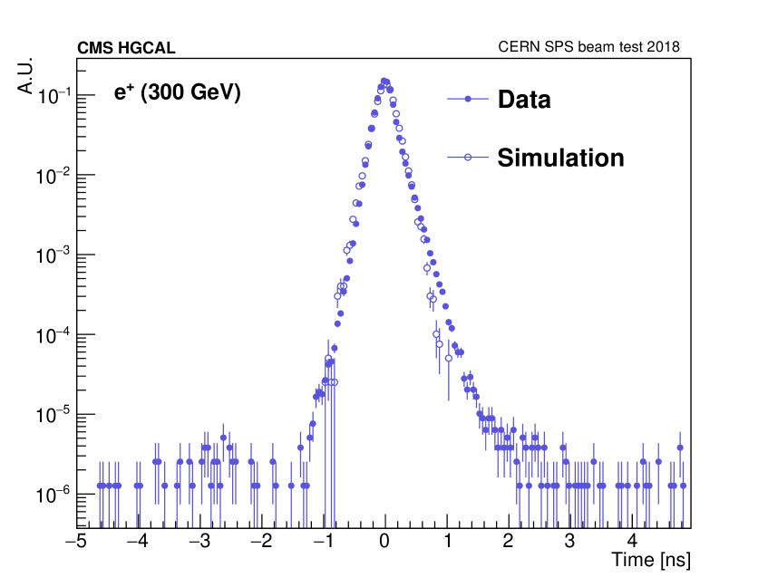
(a)

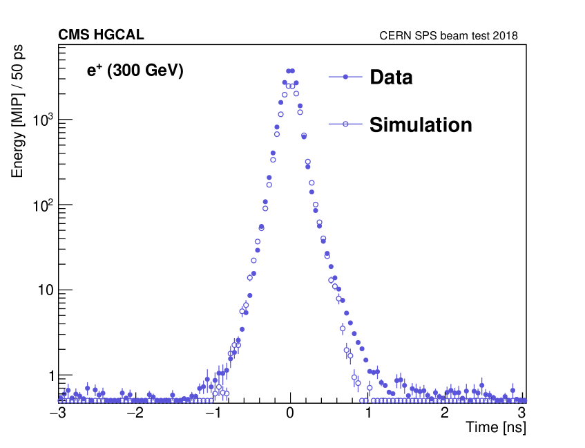
(b)

Figure 12: For the hits used in the reconstruction of the same 300 GeV positron showers, (a) time distribution of the fraction of hits and (b) the average and standard deviation of the energy of hits as a function of their calibrated time. Beam data in full markers and simulated data in empty markers.

5 Discussion and conclusion

We presented the timing performance of the first HGCAL prototype for positron showers. The focus of the analysis was to characterize the timing performance of single channels, perform measurement with full showers, and compare the results to Geant4 simulation.

After the multi-step calibration of the TOA response, $116$ readout channels in the central electromagnetic section could be fully calibrated, with an average asymptotic per-channel timing resolution of about 60, consistent with the electronics specifications. The time measurement provided by the MCP system was exploited as a reference throughout the calibration process. The MCP detector itself was measured to have a time resolution of the order of 25 for the average energy of selected positrons. An additional jitter of about 50 between the MCP and HGCAL systems was found, and its origin could not be identified. This jitter is assumed to be constant and random, such that its presence does not compromise the calibration. The timing of full positron showers was measured and compared with a simulation where the ideal timing information was smeared according to the single-channel resolution model derived from data.

The intrinsic performance of the HGCAL setup was tested by splitting the calorimeter prototype in two equivalent halves and taking the time difference between the two halves when reconstructing the same shower. The measured time resolution was found to be in agreement with simulation.

Figure 13 summarizes the measured resolution for positron showers, showing good agreement after taking into consideration the observed jitter between the MCP and HGCAL systems.

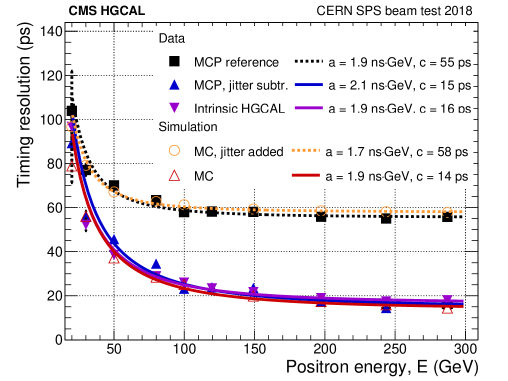
Figure 13: Comparison of the HGCAL prototype timing resolution for positron showers in data and simulated samples. For data, the resolution is measured for all layers using the MCP as a reference (black squares) as well as using only half the layers with respect to the other half and assuming they have identical resolution (purple triangles). Other measurements in the figure allow to cross-check and confirm the hypothesis that a global jitter between the MCP and HGCAL systems was present in the data.

This work represents the first measurement of HGCAL timing performance with a precision of tens of picoseconds. It also demonstrates the stability of the clock distribution used in this prototype. The results can be understood as experimental evidence of the possibility to achieve $\mathcal{O}(\qty{10}{})$ timing resolutions with the new CMS high-granularity endcap calorimeter. This timing performance is expected to enable effective separation of pile-up interactions and, with it, contribute towards a successful operation of the CMS detector at the HL-LHC.

Appendix A Example of hit timestamp calibration constants

Table 1: Example of fitted calibration constants from Equations 3.3, 3.4 and 3.5. The corresponding functions are plotted in Figures 6(a), 6(b) and 6(c). Values are rounded to their least significant digits.

Parameter	Value	Parameter	Value	Parameter	Value
$\Theta_{1,1}^{\text{TOA}}$	-14.21	$\Theta_{1,1}^{\text{TW}}$	2.97	$p_{0}$	314
$\Theta_{1,2}^{\text{TOA}}$	30.70	$\Theta_{1,2}^{\text{TW}}$	-0.73	$p_{1}$	-0.24
$\Theta_{1,3}^{\text{TOA}}$	3.62	$\Theta_{1,3}^{\text{TW}}$	-177	$p_{2}$	-2e-5□
$\Theta_{1,4}^{\text{TOA}}$	$1.253$	$\Theta_{1,4}^{\text{TW}}$	-0.8	$p_{3}$	4e-8
$\Theta_{2,1}^{\text{TOA}}$	-10.00	$\Theta_{2,1}^{\text{TW}}$	$0.05\text{\,}\mathrm{ps}\text{\,}{\mathrm{MIP}}^{-1}$	$p_{4}$	-1.2e-114
$\Theta_{2,2}^{\text{TOA}}$	$\hat{f}\left(0.65\middle|\vec{\Theta}_{1}^{TOA}\right)$	$\Theta_{2,2}^{\text{TW}}$	$\hat{f}\left(E_{\text{TOT}}\middle|\vec{\Theta}_{1}^{TW}\right)$
$\Theta_{2,3}^{\text{TOA}}$	5.53	$\Theta_{2,3}^{\text{TW}}$	-730
$\Theta_{2,4}^{\text{TOA}}$	$1.298$	$\Theta_{2,4}^{\text{TW}}$	-150

Appendix B Correlation effects

To evaluate the impact of the large in-module timing correlation discussed in Section 4.1, the full shower performance was re-evaluated by replacing Equations 4.2 and 4.3 with the more general:

$$\bar{t}=\sigma^{2}_{\bar{t}}\left(J^{T}WX\right)\mbox{ and }\sigma_{\bar{t}}^{2}=\left(J^{T}WJ\right)^{-1},$$ (B.1)

where $X=[t_{1},...,t_{n}]$, $J=[1,...,1]^{T}$, and $W=C^{-1}$, where $C$ is the covariance matrix among the $t_{i}$ measurements:

$$C=\begin{pmatrix}[c]\sigma_{1}^{2}&\ldots&\sigma_{ij}\\ \vdots&\ddots&\vdots\\ \sigma_{ij}&\ldots&\sigma_{n}^{2}\\ \end{pmatrix}\text{ , where }\sigma_{ij}=\rho\cdot\sigma_{i}\sigma_{j}=0.8\cdot\sigma_{i}^{2}\text{ for off-diagonal terms.}$$ (B.2)

The analysis was repeated following the same procedures and the obtained results differ from those shown in Figure 9 by only a few picoseconds.

The observed large correlation has a small impact on the quoted performance, and the remainder of the results reported in this paper does not include the correlation model discussed in this section.

References

- [1] CMS collaboration, The Phase-2 Upgrade of the CMS Endcap Calorimeter, Tech. Rep. CERN, Geneva (Nov, 2017), DOI.
- [2] CMS HGCAL collaboration, First beam tests of prototype silicon modules for the CMS High Granularity Endcap Calorimeter, JINST 13 (2018) P10023.
- [3] CMS HGCAL collaboration, The DAQ system of the 12,000 channel CMS high granularity calorimeter prototype, JINST 16 (2021) T04001 [2012.03876].
- [4] CMS HGCAL collaboration, Construction and commissioning of CMS CE prototype silicon modules, JINST 16 (2021) T04002 [2012.06336].
- [5] CMS HGCAL collaboration, Response of a CMS HGCAL silicon-pad electromagnetic calorimeter prototype to 20–300 GeV positrons, JINST 17 (2022) P05022 [2111.06855].
- [6] CMS, CALICE collaboration, Performance of the CMS High Granularity Calorimeter prototype to charged pion beams of 20–300 GeV/c, JINST 18 (2023) P08014 [2211.04740].
- [7] N. Charitonidis and B. Rae, “The H2 Secondary Beam Line of EHN1/SPS.” http://sba.web.cern.ch/sba/BeamsAndAreas/h2/H2manual.html, 2017.
- [8] L. Brianza et al., Response of microchannel plates to single particles and to electromagnetic showers, NIM A 797 (2015) 216.
- [9] J. Borg, S. Callier, D. Coko, F. Dulucq, C. de La Taille, L. Raux et al., SKIROC2_CMS an ASIC for testing CMS HGCAL, JINST 12 (2017) C02019.
- [10] A. Lobanov, Precision timing calorimetry with the CMS HGCAL, JINST 15 (2020) C07003.
- [11] GEANT4 collaboration, Geant4 - a simulation toolkit, NIM A 506 (2003) 250.