A fixed-point algorithm for matrix projections with applications in quantum information
Abstract
We develop a simple fixed-point iterative algorithm that computes the matrix projection with respect to the Bures distance on the set of positive definite matrices that are invariant under some symmetry. We prove that the fixed-point iteration algorithm converges exponentially fast to the optimal solution in the number of iterations. Moreover, it numerically shows fast convergence compared to the off-the-shelf semidefinite program solvers. Our algorithm, for the specific case of matrix barycenters, recovers the fixed-point iterative algorithm originally introduced in (Álvarez-Esteban et al., 2016). Compared to previous works, our proof is more general and direct as it is based only on simple matrix inequalities. Finally, we discuss several applications of our algorithm in quantum resource theories and quantum Shannon theory.
1 Introduction
Convex optimization problems play a pivotal role in various disciplines due to their mathematical structure and practical utility. In this work, we focus on a specific problem, namely computing the matrix projection with respect to the Bures distance of a positive definite matrix onto the set of positive semidefinite matrices that are invariant under a projective unitary representation of a group. We propose a simple fixed-point algorithm that recovers as a special case the fixed-point iterative algorithm for matrix barycenters in Wasserstein space originally introduced in [2]. In that work, the authors also provided the first proof of convergence for this specific case. Subsequently, in [6], a simpler proof of convergence is given, and in [10], the exponentially fast convergence in the number of iterations was proven.
The matrix barycenter problem has been studied as part of the multi-marginal transport problem or -coupling problem. Indeed, the 2-Wasserstein distance between two Gaussian measures equals the Bures distance between their covariance matrices. Moreover, the 2-Wasserstein distance is an important special case of the optimal transport problem [6]. However, our algorithm is more general and applies to several problems encountered in quantum information theory. Indeed, in quantum information theory, we are often concerned with the maximization of the fidelity function (or minimization of the Bures distance) over some constrained set.
Semidefinite programs (SDP) are a specific class of convex optimization problems with linear objective and inequality constraint functions that find several applications in many areas of research. Semidefinite programs have been widely studied during the past years and many off-the-shelf SDP solvers are available for commercial use. The matrix projection with respect to the Bures distance can be formulated as an SDP using the methods in [34]. Hence, it can be solved using SDP solvers. Moreover, the above-mentioned problem can be solved using standard mirror descent approaches such as projected gradient descent [30]. However, in its most naive application, in the range of theoretical convergence guarantees in the number of iterations, they involve the computation of a step size based on the smoothness of the function. Estimating a bound for this constant can pose a considerable challenge, as discussed, for instance, in [7, Chapter 9]. Furthermore, it typically tends to zero as the condition number diverges, making these algorithms impractical when dealing with ill-conditioned matrices. Some interesting recent works apply variations of standard mirror descent algorithms to solve very general convex problems [20, 38]. However, in their analysis, the authors do not provide convergence guarantees in the number of iterations. Nonetheless, these algorithms show very fast convergence in practice. We also mention that in [38, Section 6], inspired by the work [23], the authors consider a fixed-point algorithm that is similar to the one we develop below and they argue that it looks competitive for some specific problems and parameter ranges.
Overall, we believe that the strength of our approach is that it combines fast numerical convergence and a very simple analysis of convergence which yields strong convergence guarantees. Indeed, one inequality (Hölder’s inequality) is enough to prove convergence, and a standard strong convexity inequality (The Polyak-Łojasiewicz inequality) yields a quantitative statement in the number of iterations. Notably, the latter inequality can be employed in numerical computations to guarantee proximity to the optimal solution (see Section 7 for more details). We summarize our main contributions as follows.
-
•
In Section 3, we develop a fixed-point iterative algorithm that computes the minimum Bures distance between a positive definite matrix and a set of matrices that are invariant under a projective unitary representation of a group.
-
•
In Section 5 we provide theoretical convergence guarantees. In particular, we prove that the algorithm converges to the optimal value exponentially fast in the number of iterations. Our proof, for the specific case of matrix barycenters, recovers and greatly simplifies the one given in previous works [2, 6, 10]. Indeed, our proof is only based on simple matrix inequalities and does not involve any optimal transport inequalities.
-
•
In Section 6, we discuss several applications of our algorithms for problems in quantum resource theories and quantum Shannon theory.
- •
2 Notation
A Hermitian matrix is positive semidefinite if all its eigenvalues are nonnegative. We denote with the set of positive semidefinite matrices on a Hilvert space and we often use the notation . A Hermitian matrix is positive definite if all its eigenvalues are positive. In this case, we write . Moreover, we denote with the set of quantum states, i.e., the subset of with unit trace. The fidelity between two positive semidefinite matrices is [33]
| (1) |
The Bures distance is [8]
| (2) |
We denote with the Hilbert-Schmidt product between two Hermitian matrices . The Frobenius norm is and the fully mixed state is where is the dimension of the space. We call and the maximum and minimum eigenvalue of a positive semidefinite matrix , respectively. Given a group with projective unitary representation , we say that a matrix is symmetric if it is invariant under a projective unitary representation of a group, i.e., for any . We denote the set of symmetric positive matrices and symmetric quantum states as and , respectively.
3 Fixed-point algorithm for matrix projections with respect to the Bures distance
In this section, we introduce the matrix projection problem and the fixed-point algorithm. We also state our main theorem.
Let be a group with projective unitary representation and be a positive semidefinite matrix. Throughout this work, we want to find the positive symmetric matrix that minimizes the Bures distance to , i.e, we want to find
| (3) |
The positive symmetric matrix that solves the above optimization problem gives the projection with respect to the Bures distance of onto the set of positive symmetric matrices. We denote the group twirling
| (4) |
The fixed-point algorithm is given as follows:
In Appendix A we show that the initial point is the solution of (3) when . Moreover, we observe numerically that it generally gives a close approximation of the true solution. The main contribution of our work is to establish a theoretical convergence guarantee on the convergence of Algorithm 1.
Theorem 1.
It then follows from standard strong convexity arguments that the sequence converges to the optimal solution . We refer to subsection 5.2 and in particular to equation (23) for a discussion about the strong convexity of the Bures distance. Indeed, if we note that the gradient is zero at the minimum, -strong convexity of the Bures distance together with Theorem 1 gives
| (6) |
Here, is the strong convexity parameter of the Bures distance (see subsection 5.2).
In Theorem 1, we assume that the input positive matrix is positive, i.e., it is full-rank. If is rank-one, it is straightforward to see that the solution of (3) is given by the eigenvector corresponding to the maximum eigenvalue of multiplied by which yields the value . For non-full-rank positive semidefinite definite matrices that are not rank-one, the solution can be approximated arbitrarily well by choosing a close positive definite matrix for which we prove strong convergence guarantees. We refer to Appendix B for more details.
Remark 1.
Algorithm 1, for the specific case of matrix barycenters, recovers the fixed-point iterative algorithm originally introduced in [2]. Given a set of positive semidefinite matrices and a weight vector ; i.e., and , the matrix barycenter problem is (see [6])
| (7) |
By choosing , and where the form a one-design (e.g., the Heisenberg-Weyl operators), the optimizer of the problem (3) coincides with the matrix barycenter (7).
4 The fixed-point equation
In this section, we show that the solution of (3) for full-rank states satisfies a fixed-point equation. We note that, since the Bures distance is strongly convex in this case, the solution is unique (see Section 5.2 for more details). The fixed-point equation satisfied by the optimizer motivates the fixed-point Algorithm 1. Indeed, the optimizer is the fixed-point of the algorithm’s update.
Lemma 2.
Let be a positive definite matrix. Then is the solution of the problem (3) if and only if is positive definite and
| (8) |
Proof.
The result follows from the necessary and sufficient conditions satisfied by the optimal solution of the problem (3). We apply [26, Theorem 4] for since it is straightforward to check that the optimizer of the Bures distance problem (3) is proportional to the solution of the maximum fidelity of asymmetry of quantum states (see Section 6 for more details). Below, for completeness, we derive again the second part of the necessary and sufficient conditions of [26, Theorem 4] and show how these conditions lead to the fixed-point equation (we will now prove the support conditions). The optimizer of (3) must satisfy the support condition , where is the projection onto the support of . Since we assume that is full-rank, the support implies that the optimum is also full-rank. Hence, the optimum is achieved in the interior of the set. Since the optimizer is achieved in the set’s interior, the Frechét derivative along any symmetric Hermitian direction at the optimum is equal to zero. We introduce the shorthand . The Frechét derivative along a symmetric Hermitian direction in the symmetric point is
| (9) | ||||
| (10) |
We use that for any function and set to rewrite
| (11) |
Hence, we obtain
| (12) |
From the definition of the gradient and from the latter expression we read . To find the fixed point equation, we set the derivative in the optimal point equal to zero. Since for some Hermitian matrix , using the cyclicity of the trace, we can rewrite the condition as
| (13) |
for all Hermitain . Since this must hold for all Hermitian , we obtain the fixed-point relation
| (14) |
where we used that a symmetric positive semidefinite matrix commutes with each of the unitaries of the twirling. We then multiply both terms by on the left and the right, take the square, and multiply left and right by . This gives us the fixed-point equation for the optimum
| (15) |
∎
We now show a remarkably simple proof of convergence. In particular, we show that starting from any symmetric point, the fixed-point iteration Algorithm 1 converges to the fixed point.
5 Proof of Theorem 1
We first separately derive two inequalities. The first inequality is based on Hölder’s inequality and proves a quantitative monotonicity statement of the Bures distance to the input matrix of each iterate under the action of the fixed-point iteration. This provides a more general and simpler proof for this inequality than the one provided in [2] and [6] for the specific case of matrix barycenters which involve optimal transport inequalities. We remark that this inequality alone is sufficient to show convergence as shown in [2] and [6]. The second one is a Polyak-Łojasiewicz-type inequality which holds for strongly convex functions. We then combine these two inequalities to prove Theorem 1. Finally, we note that we actually prove a slightly stronger statement; namely, the algorithm converges to the optimum starting from any initial positive symmetric matrix.
5.1 First inequality
We have that for two Hermitian matrices and it holds
| (16) |
The equality is proved in [35, Lemma 3.21]. The inequality is a consequence of Holder’s inequality when one of the matrices is the identity (see [35, Equation 1.173]). We then set
| (17) |
so that , and . For compactness, we denote . The inequality (16) gives
| (18) | ||||
| (19) |
In the first inequality, we used that is symmetric, i.e, it commutes with any unitaries of the twirling. Hence, an additional twirling could be attached to . In the second inequality, we used that . Since the Bures distance on the left-hand side is always positive, inequality (19) also shows that the sequence produced by the fixed-point iteration has a monotonically decreasing Bures distance to .
In the following, we show that by combining the latter inequality with strong convexity arguments it is possible to derive a quantitative statement about the convergence in the number of iterations.
5.2 Second inequality
We recall that a function where is -strongly convex if it satisfies . Analogously, one can define strong convexity in the space of positive definite matrices [4]. For positive definite matrices, the Bures distance is strongly convex in the space of positive definite matrices. Indeed, we have
Theorem 3 ([5, Theorem 1]).
Let . Then for all and any Hermitian , we have
| (20) |
This means that the Bures distance is -strongly convex with and we write .
We observe that the condition is always satisfied at any step of the iteration. Indeed, we have that implies
| (21) | ||||
| (22) |
In the last step, we used that at each iteration, is symmetric and hence commutes with each unitary. Similarly, we also get that . This shows that for any and the problem does not get arbitrarily ill-conditioned. This also shows that the inverses are always well-defined at each step of the iteration since all the matrices are full-rank.
The Polyak-Łojasiewicz (PL) inequality gives the second inequality. The PL inequality for strongly convex functions bounds the difference between the function in a point with its optimal value in terms of the norm of the gradient evaluated at that point. We follow a similar approach to [16, Appendix B]. However, in our case, the optimization is performed over all symmetric matrices and it is not an unconstrained problem over . Nevertheless, we show below that the same inequality can be derived also in this context.
From Theorem 3 we know that for positive definite matrices in the compact interval , the Bures distance is strongly convex
| (23) |
Here, . We then minimize both sides of the equation with respect to in the set of positive symmetric semidefinite matrices. Note that the minimization does not change the direction of the inequality. We lower bound the minimization on the r.h.s with a minimization over the symmetric Hermitian matrices . The derivative of the r.h.s. of (23) along a Hermitian symmetric gives
| (24) |
We have that if . Therefore, the function will have only one minimum. To find the minimum, since the set of Hermitian matrices is open, we can set the derivative equal to zero. It is easy to see that the minimum in the set of Hermitian symmetric matrices is achieved by . The twirling is to ensure that is symmetric (we can also take out a twirling from ). Upon substitution, the r.h.s. becomes
| (25) |
The l.h.s just yields . We then obtain
| (26) |
where we denoted with is the optimal point and .
5.3 Combining the inequalities
Here, we show that the inequalities (19) and (26) imply that the algorithm converges exponentially fast in the number of iterations. We first note that implies that
| (27) |
We then obtain
| (28) | ||||
| (29) | ||||
| (30) |
where we denoted with the condition number of . The first inequality follows from (26), the second inequality from (27), and in the last inequality we used (19). If we denote we can rewrite the above inequality as . The latter recursive relation gives
| (31) |
which proves an exponentially fast convergence of the value of the Bures distance in the number of iterations.
Remark 2.
The constants appearing on the r.h.s. of equation (31) result from a worst-case argument. We observe that the actual constants are much smaller in practice. Whether or not a tighter analysis, at least in some regimes, could lead to better constant is still an important open problem. In particular, we note numerically that the convergence is still very fast even for very small minimum eigenvalues (and even in the limit of vanishing minimum eigenvalue).
6 Application to quantum information theory
In quantum information theory, we are often concerned with the maximization of the fidelity function over some constrained convex set. We show below that since the fidelity is connected to the Bures distance, our algorithm finds several applications in quantum information theory. In the remainder of this section, we want to find the optimal symmetric quantum state that solves the problem
| (32) |
We first show that the solutions of the problems (3) and (32) are the same up to a normalization factor. Let us set where is a positive constant and is a quantum state, i.e., . Let be a quantum state. The Bures distance between and the set of positive symmetric matrices can be written as
| (33) | ||||
| (34) |
where for the second equality we used that, for any , the optimal is given by . Therefore, the solution of the Bures minimization (3) and the solution of the fidelity maximization (32), are connected through the relationship where .
We now list some applications in quantum information theory
-
•
Fidelity of asymmetry. In resource theories, the above quantity is known as the fidelity of asymmetry. The fidelity of asymmetry quantifies the asymmetry resource of a quantum state with respect to the fidelity distance between the state and the set of symmetric states. In [18] the authors propose a quantum algorithm to test the symmetry of a quantum state whose acceptance probability is given by the fidelity of asymmetry. This endows the latter quantity with an operational meaning.
A particular instance is given by the resource theory of coherence [37] which plays a prominent role in quantum resource theories. The fidelity of coherence is an important resource measure in this resource theory [27, 21]. Explicitly, if we choose to be the cyclic group over elements with unitary representation , where is the generalized Pauli phase-shift unitary defined as , we obtain the fidelity of coherence.
-
•
Max-conditional entropy. The max-conditional entropy is a common occurrence in quantum Shannon theory [17, 31]. If we choose a one-design (e.g., the Heisenberg-Weyl operators) on the first party of a bipartite system, we obtain the max-conditional entropy [17, 31]
(35) Indeed, the action of the one-design is equivalent to the action . Moreover, the max-conditional entropy is closely related to the order- sandwiched Rényi mutual information [3, 14]
(36) Indeed, we can write
(37) (38) (39) Therefore the solution of the max-conditional entropy for the state solves the order- sandwiched Rényi mutual information of the state .
Since the matrix barycenter problem corresponds to the max-conditional entropy one for classical-quantum states as discussed at the end of Section 3, the former could be seen as a ‘fully quantum’ version of the latter.
-
•
Geometric measure of entanglement of maximally correlated states. The maximally correlated states generalize the notation of pure bipartite states and are often considered in the literature due to their properties. For example, the distillable entanglement has a closed-form expression [15] and several resource monotones become additive if at least one of the two states is of this form [26]. A maximally correlated state is a bipartite state of the form [24]
(40) The geometric measure of entanglement is , where is the fidelity of separability [36] (see also [29] for its connection with the convex-roof formulation). Here, we denoted with SEP the set of separable states.
The max-conditional entropy and the geometric measure of entanglement of maximally correlated states are connected through the relation [40, Theorem 1]. The problem is then equivalent to the computation of the max-conditional entropy discussed above.
-
•
Quantum mean state problem. We first define the quantum mean state problem introduced in [1]. Given a collection of quantum states and a probability vector , the quantum mean state problem is
(41) The quantum mean state is therefore the closest state (with respect to the fidelity) to an ensemble of quantum states. In [1], the authors discuss some applications in Bayesian quantum tomography. Moreover, in [1, Section 4.2] they show that the matrix barycenter problem is equivalent to the quantum mean state problem. As already discussed in the introduction and the remark at the end of Section 3, our analysis recovers and greatly simplifies previous proofs given for matrix barycenters and hence also applies to the quantum mean state problem.
-
•
Quantum error precompensation for group twirling channels. We first define the quantum error precompensation problem introduced in [39]. Given a quantum channel and a target state , the quantum error precompensation problem is
(42) This is the task of finding the best state to input into a quantum channel such that the corresponding output state is the closest in fidelity to a fixed target state [39]. We can use the fixed-point algorithm to find the optimal input state for the quantum error precompensation problem in the case of group twirling channels (e.g.,, the dephasing channel).
-
•
Maximum guessing probability. Let us consider a state and its purification . Moreover, let us assume that Alice holds the system and Eve holds . The fidelity of coherence of in a fixed basis gives Eve’s maximum guessing probability about Alice’s outcome after she measures in the same fixed basis [12, Section B].
7 Numerical comparison with SDP and Iterative Algorithm
In this section, we provide a numerical comparison between our fixed-point iterative algorithm and SDPT3, an off-the-shelf commercial solver available in MATLAB’s CVX package [13] that utilizes the dual interior-point method. For the fixed-point algorithm, we use the PL inequality (26) to certify the solution within an error margin. Namely, at each iteration, we compute the norm of the gradient after the group twirling which gives us an upper bound for the distance to the optimal value. We study and compare the performance of the SDP and the iterative algorithm for the max-conditional entropy and the fidelity of coherence (see Section 6 for a more detailed discussion). Explicitly, we compute the values
| (43) |
respectively. Here, is the diagonal matrix containing the elements of the diagonal of on the main diagonal. We use the SDP formulation of the fidelity given in [34] and simplify the SDP using representation theory (Schur’s lemma) [18, Section 5]. We considered bipartite quantum systems with subsystem dimensions ranging from 2 to 7 for the max-conditional entropy, and quantum states of dimensions ranging from 4 to 36 for the fidelity of coherence. For each value of the dimension, we test both algorithms on the same 100 randomly generated quantum states. The SDP solver returns a value with precision . To match the same precision, we set to the accuracy of the fixed-point algorithm. This follows from the arguments of Section 6 that relate the fidelity and the Bures distance optimizations and from the fact that the maximum fidelity to the set of symmetric states is upper bounded by the inverse of the dimension and we consider dimensions smaller than . The code is available at this link. We run both algorithms in a personal laptop with 8 GB RAM and a 2.42 GHz CPU. We compare the runtimes in Fig. 1.
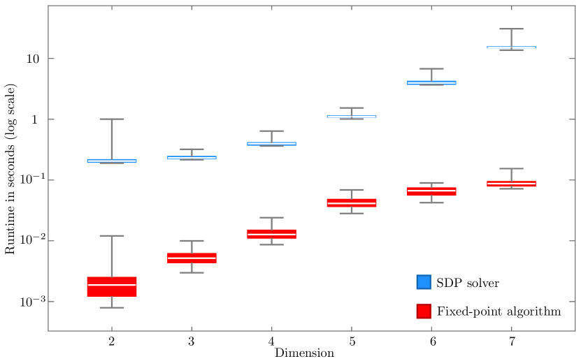
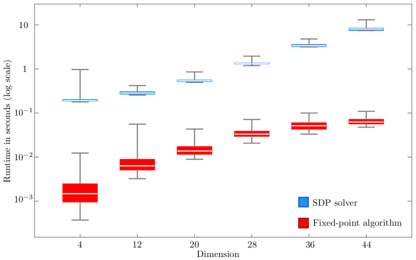
We noticed that the SDPT3 solver sometimes fails to converge within and returns an inaccurate solution. However, the fixed-point algorithm always converges. We decided to discard these samples. Fig. 1 shows that the fixed-point iterative algorithm outperforms the SDP by several orders of magnitude. Moreover, we observe that the SDP algorithm requires significantly more memory than the fixed-point one. As further evidence of the performance of our algorithm, we consider subsystem dimension in the max-conditional entropy. The SDP takes around twenty minutes while the fixed-point algorithm takes less than a second. We could not run the SDP for larger system sizes due to insufficient memory.
We also compared our map with respect to projected gradient descent [30]. According to the standard theory, we chose the step size equal to the inverse of the smoothness parameter (see e.g., [30]). We use the lower bound on the parameter in [5, Theorem 1]. We note that even though the performance is similar to the SDP one for small dimensions, for higher dimensions it performs worse.
8 Further directions
Our numerical simulations suggest that similar algorithms could be used to solve analogous problems for different families of quantum Rényi divergences [31], double optimization problems as the Rényi mutual information in [19], and quantum error precompensation for more general quantum channels [39] (e.g., depolarizing channel). Finally, one could try to include more general constraints in the analysis by similarly projecting at each iteration onto the set of feasible solutions. We have numerical evidence that such fixed-point algorithms perform well in practice; however, it appears that a theoretical investigation of convergence guarantees for such problems requires additional techniques and we leave this as an open question.
9 Acknowledgment
The authors would like to thank Hao-Chung Cheng, Mario Berta, Richard Kueng, Ian George, Erkka Haapasalo, and Antonios Varvitsiotis for discussions. In particular, we thank Christoph Hirche for suggestions at an earlier stage of the project. SB, RR, and MT were supported by the National Research Foundation, Singapore, and A*STAR under its CQT Bridging Grant. In the latter stages of the work, SB was supported by Duke University’s ECE Departmental fellowship. MT is also supported by the National Research Foundation, Singapore, and A*STAR under its Quantum Engineering Programme (NRF2021-QEP2-01-P06). This research is also supported by the Quantum Engineering Programme grant NRF2021-QEP2-02-P05.
References
- [1] A. Afham, R. Kueng, and C. Ferrie. “Quantum mean states are nicer than you think: fast algorithms to compute states maximizing average fidelity”. arXiv:2206.08183 , (2022).
- [2] P. C. Álvarez-Esteban, E. Del Barrio, J. Cuesta-Albertos, and C. Matrán. “A fixed-point approach to barycenters in Wasserstein space”. Journal of Mathematical Analysis and Applications 441(2): 744–762 (2016).
- [3] S. Beigi. “Sandwiched Rényi divergence satisfies data processing inequality”. Journal of Mathematical Physics 54(12) (2013).
- [4] R. Bhatia. “Matrix analysis, volume 169 of”. Graduate texts in mathematics , (1997).
- [5] R. Bhatia, T. Jain, and Y. Lim. “Strong convexity of sandwiched entropies and related optimization problems”. Reviews in Mathematical Physics 30(09): 1850014 (2018).
- [6] R. Bhatia, T. Jain, and Y. Lim. “On the Bures–Wasserstein distance between positive definite matrices”. Expositiones Mathematicae 37(2): 165–191 (2019).
- [7] S. P. Boyd and L. Vandenberghe. Convex optimization. Cambridge university press (2004).
- [8] D. Bures. “An extension of Kakutani’s theorem on infinite product measures to the tensor product of semifinite -algebras”. Transactions of the American Mathematical Society 135: 199–212 (1969).
- [9] E. Carlen. “Trace inequalities and quantum entropy: an introductory course”. Entropy and the quantum 529: 73–140, (2010).
- [10] S. Chewi, T. Maunu, P. Rigollet, and A. J. Stromme. “Gradient descent algorithms for Bures-Wasserstein barycenters”. In Conference on Learning Theory, pages 1276–1304, (2020).
- [11] E. Chitambar and G. Gour. “Comparison of incoherent operations and measures of coherence”. Physical Review A 94(5): 052336 (2016).
- [12] P. J. Coles. “Unification of different views of decoherence and discord”. Physical Review A 85(4): 042103 (2012).
- [13] M. Grant and S. Boyd. “CVX: Matlab software for disciplined convex programming, version 2.1”, (2014).
- [14] M. K. Gupta and M. M. Wilde. “Multiplicativity of completely bounded p-norms implies a strong converse for entanglement-assisted capacity”. Communications in Mathematical Physics 334: 867–887 (2015).
- [15] M. Horodecki, P. Horodecki, and R. Horodecki. “Limits for entanglement measures”. Physical Review Letters 84(9): 2014 (2000).
- [16] H. Karimi, J. Nutini, and M. Schmidt. “Linear convergence of gradient and proximal-gradient methods under the polyak-łojasiewicz condition”. In Machine Learning and Knowledge Discovery in Databases: European Conference, ECML PKDD 2016, Riva del Garda, Italy, September 19-23, 2016, Proceedings, Part I 16, pages 795–811, (2016).
- [17] R. Konig, R. Renner, and C. Schaffner. “The operational meaning of min-and max-entropy”. IEEE Transactions on Information theory 55(9): 4337–4347 (2009).
- [18] M. L. LaBorde, S. Rethinasamy, and M. M. Wilde. “Testing symmetry on quantum computers”. arXiv:2105.12758 (2021).
- [19] K. Li and Y. Yao. “Operational Interpretation of the Sandwiched Rényi Divergences of Order 1/2 to 1 as Strong Converse Exponents”. arXiv:2209.00554 , (2022).
- [20] Y.-H. Li and V. Cevher. “Convergence of the exponentiated gradient method with Armijo line search”. Journal of Optimization Theory and Applications 181(2): 588–607 (2019).
- [21] C. Liu, D.-J. Zhang, X.-D. Yu, Q.-M. Ding, and L. Liu. “A new coherence measure based on fidelity”. Quantum Information Processing 16: 1–10 (2017).
- [22] A. Marwah and F. Dupuis. “Uniform continuity bound for sandwiched Rényi conditional entropy”. Journal of Mathematical Physics 63(5): 052201 (2022).
- [23] B. Nakiboğlu. “The Augustin capacity and center”. Problems of Information Transmission 55: 299–342, (2019).
- [24] E. M. Rains. “Bound on distillable entanglement”. Phys. Rev. A 60(1): 179 (1999).
- [25] R. Rubboli and M. Tomamichel. “Fundamental limits on correlated catalytic state transformations”. Physical Review Letters 129(12): 120506 (2022).
- [26] R. Rubboli and M. Tomamichel. “New additivity properties of the relative entropy of entanglement and its generalizations”. arXiv:2211.12804 , (2022).
- [27] L.-H. Shao, Z. Xi, H. Fan, and Y. Li. “Fidelity and trace-norm distances for quantifying coherence”. Physical Review A 91(4): 042120 (2015).
- [28] N. Sharma and N. A. Warsi. “Fundamental bound on the reliability of quantum information transmission”. Physical review letters 110(8): 080501 (2013).
- [29] A. Streltsov, H. Kampermann, and D. Bruß. “Linking a distance measure of entanglement to its convex roof”. New. J. Phys. 12(12): 123004 (2010).
- [30] M. Teboulle. “A simplified view of first order methods for optimization”. Mathematical Programming 170(1): 67–96 (2018).
- [31] M. Tomamichel. Quantum information processing with finite resources: mathematical foundations. volume 5, Springer (2015).
- [32] M. Tomamichel, M. Berta, and M. Hayashi. “Relating different quantum generalizations of the conditional Rényi entropy”. Journal of Mathematical Physics 55(8) (2014).
- [33] A. Uhlmann. “The Transition Probability for States of Star- Algebras”. Annalen der Physik 497(4-6): 524–532 (1985).
- [34] J. Watrous. “Simpler semidefinite programs for completely bounded norms”. arXiv:1207.5726 , (2012).
- [35] J. Watrous. The theory of quantum information. Cambridge university press (2018).
- [36] T.-C. Wei and P. M. Goldbart. “Geometric measure of entanglement and applications to bipartite and multipartite quantum states”. Phys. Rev. A 68(4): 042307 (2003).
- [37] A. Winter and D. Yang. “Operational resource theory of coherence”. Physical review letters 116(12): 120404 (2016).
- [38] J.-K. You, H.-C. Cheng, and Y.-H. Li. “Minimizing quantum Rényi divergences via mirror descent with Polyak step size”. In 2022 IEEE International Symposium on Information Theory (ISIT), pages 252–257, (2022).
- [39] C. Zhang, L. Li, G. Lu, H. Yuan, and R. Duan. “Quantum error precompensation for quantum noisy channels”. Physical Review A 106(4): 042440 (2022).
- [40] H. Zhu, M. Hayashi, and L. Chen. “Coherence and entanglement measures based on Rényi relative entropies”. J. Phys. A: Mathematical and Theoretical 50(47): 475303 (2017).
Appendices
A Optimal choice of the initial point
In this appendix, we show that the initial point of our fixed-point algorithm is the solution of a quantity that is closely related to the Bures distance. Our choice is motivated by the fact that, as we describe below, in some special cases the two problems are equal. Moreover, we numerically observe that the initial point often provides a good approximation of the optimizer of the original problem. Let . We define
| (44) |
This quantity is related to the Petz Rényi relative entropy of order (see e.g., [31] for a review) and is equal to the Bures distance if the two matrices commute. In the remaining part of this appendix, we will be concerned with the minimization problem
| (45) |
The problem (45) is similar to the one in (3) where is replaced by . However, the above problem admits a closed-form solution; the optimal positive semidefinite matrix is given by . We now prove this statement. As usual, we also use the notation . Following a similar approach to Section 6, it is straightforward to prove that the solution of (45) is proportional to a similar minimization problem which involves the Petz Rényi relative entropy of order . We can then use the results of [26, Theorem 4]. The necessary and sufficient conditions of the optimizer are and
| (46) |
for any Hermitian and symmetric . We then use the ansatz . Here, denotes the projector onto the support of . Note that the ansatz always satisfies the support condition since the group twirling contains the identity element. Using the ansatz, inequality (46) becomes for any Hermitian . The latter inequality is always satisfied since . This proves that the ansatz is the optimizer. This generalizes the known result for the Petz conditional entropies of order [28, 32] and the Petz coherence measures of order [11]. In the specific case that the input matrix commutes with its optimizer, i.e., , the necessary and sufficient conditions for the optimizer of the problem (45) and the original one for the Bures distance (3) become the same [26, Corollary 5]. Hence, in this situation, the solution of the two problems coincide. In other words, whenever , the positive semidefinite matrix is the solution of the original Bures problem (3). As an explicit example, let us consider the matrix barycenter problem when all the matrices commute among themselves. In this case, the latter commutation relation is satisfied and hence the solution coincides with the initial point of our algorithm. The solution is the power means as already pointed out in [6].
B Continuity bound for non-full-rank input positive semidefinite matrices
If the input matrix is not full-rank, we cannot apply Theorem 1. However, we could consider full-rank matrices that are arbitrarily close to it for which the theorem still holds. Indeed, for these matrices, we can give strong convergence guarantees. In the following, we derive a continuity bound that bounds the error we make using this approximation. Explicitly, we can run the algorithm on a slightly depolarized matrix and approximate the true value arbitrarily well. Here, is the dimension of . We note that for a small value of the condition number gets very large. This could make the convergence to the solution very slow. However, in practice, as discussed at the end of Section 5.3, we find that even for small values of the algorithm converges to the solution very fast. It is easy to check that the trace distance can be bounded as
| (47) |
We then have
Proposition 4.
Let . Then for any such that and we have
| (48) |
Proof.
We follow a similar proof to the one given in [25, Supplemental material - Corollary 4]. We first note that
| (49) |
where we denoted with the optimizer of . Since the upper bound in the proposition is a function of we can assume the worst-case scenario and set . We set where and are the positive and negative parts, respectively. We then have
| (50) | ||||
| (51) |
where in the last equality of (51) we used (50). It follows that . We define the normalized positive semidefinite matrix . We then use that and we obtain
| (52) | ||||
| (53) | ||||
| (54) | ||||
| (55) |
where in (53) we used that the trace functional inherits the monotonicity from (see e.g., [9]) and in (54) we used that for two positive semidefinite matrices and and it holds [4, 22]. The last implication (55) follows from the inequality
| (56) |
since the fidelity of two states is upper-bounded by and, as we show in Section 6, . Here, we denoted . The above relation also holds if we exchange and . ∎