Likelihood for a Network of Gravitational-Wave Detectors with Correlated Noise

Abstract

The Einstein Telescope faces a critical data analysis challenge with correlated noise, often overlooked in current parameter estimation analyses. We address this issue by presenting the statistical formulation of the likelihood function that includes correlated noise for the Einstein Telescope or any detector network. Neglecting these correlations may significantly reduce parameter estimation accuracy, even leading to the failure to reconstruct otherwise resolvable signals. This emphasizes how critical a proper treatment of correlated noise is, as presented in this work, to unlocking the wealth of results promised by the Einstein Telescope.

I Introduction

The second-generation of interferometers has detected a large number of coalescing binaries [1, 2, 3, 4, 5], enabling groundbreaking scientific results. The next-generation of gravitational-wave (GW) detectors promises to open up new frontiers in the exploration of the Universe, making it possible to address a variety of problems in astrophysics, fundamental physics, and cosmology [16, 24, 8, 18, 6].
The European proposal for a third-generation ground-based detector is represented by Einstein Telescope (ET) [26]. The proposed geometry for ET consists of six-in-one co-located interferometers (three specialized in the low-frequency observations, three in the high-frequency), with an opening angle of $\pi/3$, disposed underground in a triangular shape.
Due to the small distance between the input/output test masses of different interferometers [17], non-negligible correlations in the noise among its detectors are expected. These correlations arise mainly in the form of magnetic [22, 23], seismic and Newtonian noise [21], and could highly limit all kinds of unmodeled searches which rely on cross-correlating data, such as searches for the stochastic GW background [27, 9].
Although the presence of correlated noise has been widely recognized by the GW community, it is usually neglected in the context of parameter estimation (PE) analysis, where different detectors forming a network are assumed to be uncorrelated [28, 10]. Several techniques have been developed to subtract these correlations or mitigate their impact [11, 12, 7], improving the detector sensitivity and the subsequent estimation of source parameters [15, 13].

The flagship results for ET necessitate precise PE analysis, such as testing General Relativity, probing neutron star equations of state or inferring cosmological parameters. Similarly, searches for a stochastic background of GWs, signals from core-collapse supernovae and rotating neutron stars rely on an accurate identification of resolved signals. Nevertheless, the presence of correlated noise will have a significant impact on achieving this. Without proper treatment, we may threaten the scientific potential of ET.
Differently from the existing literature, we address the issue of including correlated noise directly in the PE analysis. We present a statistical derivation of the likelihood function, both in its time and frequency-domain, for analyzing GW data with a network of correlated detectors. We investigate the consequences of neglecting correlated noise in ET by considering the scenario of interferometers (almost) maximally correlated. Importantly, we show a significant drop in the PE accuracy for a simulated signal close to the detection threshold. The main goal of this paper is to emphasize that ignoring correlations in PE analysis can undermine the wealth of results expected from ET, stressing the importance of using a likelihood function that accounts for correlations.

II Likelihood Function Formulation

In the context of GW data analysis, one of the pivotal elements is the likelihood function $p(\boldsymbol{d}|\boldsymbol{\theta})$, which represents the probability density function of the observed data $\boldsymbol{d}$ given a set of parameters $\boldsymbol{\theta}$. Failing in an accurate construction endangers robust PE and hypothesis testing. Here, we present a statistical formulation of the likelihood function for ET addressing the issue of including noise correlations among different detectors. For the purpose of the analysis, we ignore the details of the xylophone configuration [20] and treat ET as consisting of three interferometers. However, the following derivation and results can be generalized straightforwardly to any network of GW interferometers.

II.1 Time-domain representation of the likelihood function for correlated noise

Within a network of GW interferometers, we indicate with $\boldsymbol{n}_{j}=[n_{j}(t_{N-1}),\dots,n_{j}(t_{0})]^{T}$ the noise time series for the $j\text{-th}$ interferometer, assuming a sampling frequency of $1/\Delta t$. In particular, we consider the time-reversed version of the standard time series definition for consistency with other definitions. We make the usual assumption that the noise in each interferometer is Gaussian and wide-sense stationary, meaning that it is fully described by its mean $\mathbb{E}[\boldsymbol{n}_{j}]$, which can be arbitrarily set to zero, and by its covariance, which depends only on the time lag between two noise realizations.

Conventionally, the noise time series of multiple interferometers are expressed as a matrix $\boldsymbol{N}\in\mathbb{R}^{3\times N}$, with each row $j$ corresponding to the time series of the $j\text{-th}$ interferometer. To facilitate the characterization of the spatial and temporal correlation, we introduce the vectorized noise time series defined as follows

$$\boldsymbol{n}\coloneq\text{vec}(\boldsymbol{N}^{T})=\begin{bmatrix}\boldsymbol{n}_{1}\\ \boldsymbol{n}_{2}\\ \boldsymbol{n}_{3}\end{bmatrix}$$ (1)

where $\boldsymbol{n}\in\mathbb{R}^{3N}$. We define the cross covariance between the noise in the $j\text{-th}$ and the $j^{\prime}\text{-th}$ detectors as $C_{jj^{\prime},n}=\mathbb{E}[n_{j}(t)\hskip 2.0ptn_{j^{\prime}}(t+t_{n})]$, from which

$$\boldsymbol{\Sigma}_{jj^{\prime}}\hskip 3.0pt \coloneq\mathbb{E}\left[\boldsymbol{n}_{j}^{T}\boldsymbol{n}_{j^{\prime}}\right]$$ (2a)

$$=\begin{pmatrix}C_{jj^{\prime},0}&C_{jj^{\prime},-1}&\dots&C_{jj^{\prime},-(N-1)}\\ C_{jj^{\prime},1}&C_{jj^{\prime},0}&\dots&C_{jj^{\prime},-(N-2)}\\ \vdots&\vdots&\ddots&\vdots\\ C_{jj^{\prime},N-1}&C_{jj^{\prime},N-2}&\dots&C_{jj^{\prime},0}\\ \end{pmatrix}$$ (2b)

$\boldsymbol{\Sigma}_{jj^{\prime}}$ is the $N\times N$ noise (cross)covariance matrix. It assumes a Toeplitz form for $j\neq j^{\prime}$ and a symmetric Toeplitz form for $j=j^{\prime}$. The spatial and temporal correlation of the noise process $\boldsymbol{n}$ are characterized by the $3N\times 3N$ network covariance matrix $\boldsymbol{\Sigma}$, given by

$$\boldsymbol{\Sigma} :=\mathbb{E}\left[\boldsymbol{n}^{T}\boldsymbol{n}\right]$$ (3a)

$$=\begin{bmatrix}\mathbb{E}\left[\boldsymbol{n}_{1}^{T}\boldsymbol{n}_{1}\right]&\mathbb{E}\left[\boldsymbol{n}_{1}^{T}\boldsymbol{n}_{2}\right]&\mathbb{E}\left[\boldsymbol{n}_{1}^{T}\boldsymbol{n}_{3}\right]\\ \mathbb{E}\left[\boldsymbol{n}_{2}^{T}\boldsymbol{n}_{1}\right]&\mathbb{E}\left[\boldsymbol{n}_{2}^{T}\boldsymbol{n}_{2}\right]&\mathbb{E}\left[\boldsymbol{n}_{2}^{T}\boldsymbol{n}_{3}\right]\\ \mathbb{E}\left[\boldsymbol{n}_{3}^{T}\boldsymbol{n}_{1}\right]&\mathbb{E}\left[\boldsymbol{n}_{3}^{T}\boldsymbol{n}_{2}\right]&\mathbb{E}\left[\boldsymbol{n}_{3}^{T}\boldsymbol{n}_{3}\right]\end{bmatrix}$$ (3b)

$$=\begin{bmatrix}\boldsymbol{\Sigma}_{11}&\boldsymbol{\Sigma}_{12}&\boldsymbol{\Sigma}_{13}\\ \boldsymbol{\Sigma}_{21}&\boldsymbol{\Sigma}_{22}&\boldsymbol{\Sigma}_{23}\\ \boldsymbol{\Sigma}_{31}&\boldsymbol{\Sigma}_{32}&\boldsymbol{\Sigma}_{33}\end{bmatrix}$$ (3c)

The diagonal blocks characterize the temporal correlation of the noise process in each detector, and the off-diagonal blocks characterize the spatial correlation of the noise processes between different detectors. For the off-diagonals blocks $\boldsymbol{\Sigma}_{jj^{\prime}}=\boldsymbol{\Sigma}_{j^{\prime}j}^{T}$.

Let us consider the hypothesis that the data $\boldsymbol{d}$ recorded by ET contain a GW signal depending on a set of source parameters $\boldsymbol{\theta}$. We model the output as

$$\boldsymbol{d}=\boldsymbol{s}(\boldsymbol{\theta})+\boldsymbol{n}$$ (4)

where $\boldsymbol{s}(\boldsymbol{\theta})$ and $\boldsymbol{n}$ are the GW signal component and the noise component, respectively. For such a hypothesis, the time-domain likelihood function of observing the data set $\boldsymbol{d}$ follows the distribution of the noise. In particular, it is given by a multivariate normal distribution

$$p(\boldsymbol{d}|\boldsymbol{\theta})=\dfrac{1}{|2\pi\boldsymbol{\Sigma}|^{1/2}}\exp{\bigg{[}-\frac{1}{2}(\boldsymbol{d}}-\boldsymbol{s}(\boldsymbol{\theta}))^{T}\boldsymbol{\Sigma}^{-1}(\boldsymbol{d}-\boldsymbol{s}(\boldsymbol{\theta}))\bigg{]}$$ (5)

which corresponds to the maximum entropy distribution of the zero-mean noise processes constrained by the network covariance matrix $\boldsymbol{\Sigma}$.

II.2 Frequency-domain representation of the likelihood function for correlated noise

Although the time domain formulation is essential for understanding the data as it is recorded, given the reduced complexity it is useful to present the frequency-domain version of Eq. (5). Let $\boldsymbol{S}$ be the spectral matrix defined as follows

$$\boldsymbol{S}\coloneq\begin{bmatrix}\boldsymbol{S}_{11}&\boldsymbol{S}_{12}&\boldsymbol{S}_{13}\\ \boldsymbol{S}_{21}&\boldsymbol{S}_{22}&\boldsymbol{S}_{23}\\ \boldsymbol{S}_{31}&\boldsymbol{S}_{32}&\boldsymbol{S}_{33}\end{bmatrix}$$ (6)

where

$$S_{jj^{\prime}}(f_{k})=2\Delta t\sum_{n=0}^{N-1}C_{jj^{\prime},n}\hskip 3.0pte^{-2\pi ikn/N}$$ (7a)

$$\boldsymbol{S}_{jj^{\prime}}=\text{diag}(S_{jj^{\prime}}(f_{0}),\dots,S_{jj^{\prime}}(f_{N-1}))$$ (7b)

In particular, $S_{jj}(f_{k})$ is the $k\text{-th}$ component of the one-sided Power Spectral Density (PSD) for the $j\text{-th}$ interferometer, and $S_{jj^{\prime}}(f_{k})$ the $k\text{-th}$ component of the one-sided Cross Power Spectral Density (CSD) between the $j\text{-th}$ and the $j^{\prime}\text{-th}$ interferometers. Note that $\boldsymbol{S}_{jj^{\prime}}=\boldsymbol{S}_{j^{\prime}j}^{*}$.
It can be shown [19] that each (cross)covariance Toeplitz matrix $\boldsymbol{\Sigma}_{jj^{\prime}}$ is asymptotically equivalent to a circulant matrix, meaning that its eigenvalues are the Discrete Fourier Transform (DFT) of the first column. In other words, each block of $\boldsymbol{\Sigma}$ can be independently diagonalized by the DFT basis, resulting in the corresponding (Cross)PSD matrix. This yields the following frequency-domain representation of the likelihood function

$$p(\boldsymbol{d}|\boldsymbol{\theta})=\dfrac{1}{|\pi\boldsymbol{S}/2\Delta f|^{1/2}}\exp{\bigg{[}-2\Delta f(\tilde{\boldsymbol{d}}}-\tilde{\boldsymbol{s}}(\boldsymbol{\theta}))^{\dagger}\hskip 3.0pt\boldsymbol{S}^{-1}\hskip 3.0pt(\tilde{\boldsymbol{d}}-\tilde{\boldsymbol{s}}(\boldsymbol{\theta}))\bigg{]}$$ (8)

where $\Delta f=1/N\Delta t$ is the frequency resolution, the dagger $(\dagger)$ represents the conjugate transpose, and the tilde on $\tilde{\boldsymbol{d}}$ denotes that the DFT is applied on each individual row of the matrix $\boldsymbol{D}\in\mathbb{R}^{3\times N}$ (the same applies for $\tilde{\boldsymbol{s}}(\boldsymbol{\theta})$). Since the entries of $\boldsymbol{S}$ are diagonal matrices, the inverse of $\boldsymbol{S}$ also follows the same structure.
One can rewrite Eq. (8) in the more compact form

$$p(\boldsymbol{d}|\boldsymbol{\theta})=\dfrac{1}{|\pi\boldsymbol{S}/2\Delta f|^{1/2}}\hskip 5.0pte^{-\frac{1}{2}(\boldsymbol{d}-\boldsymbol{s}(\boldsymbol{\theta})\hskip 1.0pt|\hskip 1.0pt\boldsymbol{d}-\boldsymbol{s}(\boldsymbol{\theta}))}$$ (9)

where $\big{(}\boldsymbol{x}\hskip 1.0pt|\hskip 1.0pt\boldsymbol{x}\big{)}$ is the noise-weighted inner product of the network time series $\boldsymbol{x}$ with itself, defined as

$$\big{(}\boldsymbol{x}\hskip 1.0pt|\hskip 1.0pt\boldsymbol{x}\big{)}:=4\Delta f\hskip 4.0pt\Re\Bigg{(}\sum_{j,j^{\prime}=1}^{3}\sum_{k}\tilde{x}_{j}^{*}(f_{k})\hskip 3.0pt(\boldsymbol{S}^{-1})_{jj^{\prime}}(f_{k})\hskip 3.0pt\tilde{x}_{j^{\prime}}(f_{k})\Bigg{)}$$ (10)

In particular, $(\boldsymbol{S}^{-1})_{jj^{\prime}}(f_{k})$ denotes the $k\text{-th}$ diagonal entry of the block $jj^{\prime}$ of the inverse of $\boldsymbol{S}$. The index $k$ varies from the DC frequency at $k=0$ to the Nyquist frequency at $k=N/2-1$, both extremes excluded.

II.3 Likelihood function for uncorrelated noise

In the case of uncorrelated detectors, the off-diagonal blocks in the network covariance matrix $\boldsymbol{\Sigma}$ and in the spectral matrix $\boldsymbol{S}$ vanish, that is

$$\boldsymbol{\Sigma}^{\text{uncorr}} \coloneq\begin{bmatrix}\boldsymbol{\Sigma}_{11}&\boldsymbol{0}&\boldsymbol{0}\\ \boldsymbol{0}&\boldsymbol{\Sigma}_{22}&\boldsymbol{0}\\ \boldsymbol{0}&\boldsymbol{0}&\boldsymbol{\Sigma}_{33}\end{bmatrix}$$ (11a)

$$\boldsymbol{S}^{\text{uncorr}} \coloneq\begin{bmatrix}\boldsymbol{S}_{11}&\boldsymbol{0}&\boldsymbol{0}\\ \boldsymbol{0}&\boldsymbol{S}_{22}&\boldsymbol{0}\\ \boldsymbol{0}&\boldsymbol{0}&\boldsymbol{S}_{33}\end{bmatrix}$$ (11b)

For this specific case, the time-domain representation of the likelihood function in Eq. (5) is simply given by the product of the single detector likelihoods

$$p(\boldsymbol{d}|\boldsymbol{\theta})\propto\prod_{j=1}^{3}\exp{\bigg{[}-\frac{1}{2}(\boldsymbol{d}_{j}-\boldsymbol{s}_{j}(\boldsymbol{\theta}))^{T}(\boldsymbol{\Sigma}_{jj})^{-1}(\boldsymbol{d}_{j}-\boldsymbol{s}_{j}(\boldsymbol{\theta}))\bigg{]}}$$ (12)

The same goes for the frequency-domain representation in Eq. (8), which reduces to the product of the Whittle likelihoods for each detector $j$

$$p(\boldsymbol{d}|\boldsymbol{\theta})\propto\prod_{j=1}^{3}\exp{\bigg{[}-2\Delta f(\tilde{\boldsymbol{d}}_{j}-\tilde{\boldsymbol{s}}_{j}(\boldsymbol{\theta}))^{\dagger}(\boldsymbol{S}_{jj})^{-1}(\tilde{\boldsymbol{d}}_{j}-\tilde{\boldsymbol{s}}_{j}(\boldsymbol{\theta}))\bigg{]}}$$ (13)

III Parameter Estimation in the presence of correlated noise

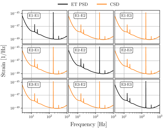
Figure 1: Graphical representation of the spectral matrix $\boldsymbol{S}$ used in the analysis. In particular, we refer to the three ET interferometers as E1, E2 and E3. The diagonal blocks of $\boldsymbol{S}$ contain ET PSD for each detector (black), while the off-diagonal blocks contain the CSD used in the analysis for each detector pair (orange), corresponding to the $90\%$ of ET PSD. Since we are assuming the noise to be in-phase among every interferometer, the off-diagonal blocks are real-valued and the spectral matrix is symmetric.

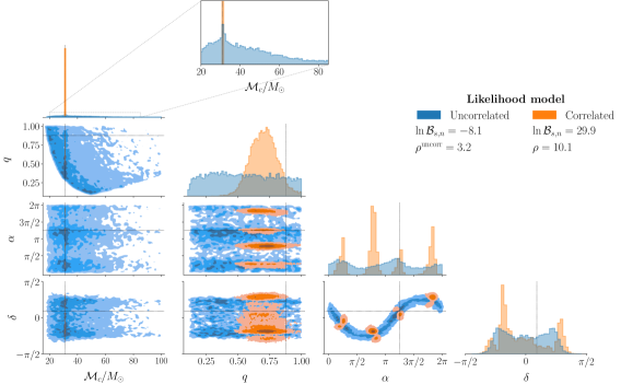
Figure 2: Posterior distributions for the chirp mass $\mathcal{M}_{c}$, the mass ratio $q$, the right ascension $\alpha$ and the declination $\delta$, for different likelihood models (color). Contours in the 2D plots enclose the 10%, 50% and 90% of the probability mass, and the dashed lines represent the injected values. The inset displays a zoom of the chirp mass’ posterior distribution. Only the analysis performed with the correlated likelihood reconstructs the GW signal.

To demonstrate the impact of ignoring correlated noise, we consider the scenario in which ET interferometers are (almost) maximally correlated. We perform a PE analysis of a synthetic binary black hole (BBH) signal with the ‘correlated’ likelihood (Eq. (8)) and the ‘uncorrelated’ likelihood (Eq. (13)), to investigate how the GW signal is reconstructed by the two models. The analysis is performed in the frequency domain by means of the software package granite [14]

III.1 Spectral matrix setup

In a realistic scenario for ET, the $\boldsymbol{S}$ matrix is composed of the estimated PSDs for each interferometer and of the estimated CSDs for each interferometer pair. Estimating the PSDs involves auto-correlating the strain from each individual detector; similarly, to obtain an estimate of the CSDs all that is needed, in principle, is to cross-correlate the strain of data measured by each detector. In our simulation, we assume the same PSD for every detector, equivalent to the design sensitivity of the xylophone configuration [20], $S_{\text{ET}}$, i.e.

$$S_{jj}(f_{k})=S_{\text{ET}}(f_{k})\hskip 20.0ptj=1,2,3$$ (14)

We express the CSD in terms of the correlation coefficients as follows

$$S_{jj^{\prime}}(f_{k})=c_{jj^{\prime}}(f_{k})\hskip 2.0pt\sqrt{S_{jj}(f_{k})\hskip 3.0ptS_{j^{\prime}j^{\prime}}(f_{k})}$$ (15)

where $c_{jj^{\prime}}(f_{k})\in\mathbb{C}$ describe the correlation between the detectors $j$ and $j^{\prime}$. We assume the noise in the interferometers to be (almost) fully correlated and in-phase all over the sensitivity frequency band, that is

$$|c_{jj^{\prime}}| =0.9$$ (16a)

$$\angle c_{jj^{\prime}} =1$$ (16b)

for each frequency component $k$. In particular, the value of $0.9$ is selected to avoid unwanted numerical effects in the inversion of $\boldsymbol{S}$. With the expression for $S_{jj}(f_{k}),\hskip 3.0ptS_{jj^{\prime}}(f_{k})$ we construct the $\boldsymbol{S}_{jj},\hskip 3.0pt\boldsymbol{S}_{jj^{\prime}}$ matrices and the spectral matrix $\boldsymbol{S}$ as in Eq. (6). Similarly, we construct $\boldsymbol{S}^{\text{uncorr}}$, defined in Eq. (11b). A graphical representation of the spectral matrix used in the analysis is sketched in Fig. 1.

III.2 Mock data generation

We produce the mock data for ET generating the correlated noise from a zero-mean multivariate normal distribution, with $\boldsymbol{S}/2$ as the covariance matrix. The real and imaginary parts are generated independently, and summed to obtain the network frequency series $\tilde{\boldsymbol{n}}$. Precisely, we select a sampling frequency of $1/\Delta t=512\text{ Hz}$ and we discard all the frequencies below $6\text{ Hz}$ and above the Nyquist frequency $1/2\Delta t$. Finally, we generate a synthetic BBH signal with the IMRPhenomXPHM frequency-domain model [25], and we inject it into the noise series $\tilde{\boldsymbol{n}}$.

III.3 Network Signal-to-Noise Ratio (SNR) for correlated noise

In the context of matched filtering, the optimal value of the SNR for a single detector analysis is defined as

$$\rho_{j}=\sqrt{4\Delta f\hskip 4.0pt\Re\Bigg{(}\sum_{k}\dfrac{|\tilde{s}_{j}(f_{k})|^{2}}{S_{jj}(f_{k})}\Bigg{)}}$$ (17)

where $\tilde{s}_{j}(f_{k})$ is the $k\text{-th}$ frequency component of the GW signal detected in the $j\text{-th}$ interferometer. From Eq. (10), we generalize the expression to the case of a network analysis with correlated noise as follows

$$\rho\coloneq\big{(}\boldsymbol{s}\hskip 1.0pt|\hskip 1.0pt\boldsymbol{s}\big{)}^{1/2}$$ (18)

where $\boldsymbol{s}(\boldsymbol{\theta})$ is the network time series of the detected GW signal. Note once again that for uncorrelated detectors, Eq. (18) reduces to the usual quadrature sum of the SNR for each detector, $\rho^{\text{uncorr}}=\big{(}\sum_{j=1}^{3}\rho_{j}^{2}\big{)}^{1/2}$.

Using the above expressions, we calculate the injected SNR for the analyzed GW signal. Specifically, we find $\rho=10.1$ accounting for noise correlations among ET interferometers and $\rho^{\text{uncorr}}=3.2$ under the assumption of uncorrelated detectors. The disparity between these values is due to the nature of correlated noise itself, which enhances the collective information about noise processes, akin to a network of witness sensors measuring the same physical phenomenon. This implies the better efficacy of spectral component weighting in the SNR calculation. One can regard this finding as an indication of the higher accuracy of the correlated likelihood in the PE analysis, as detailed in the next section.

III.4 Comparison between correlated and uncorrelated likelihood function

Fig. 2 shows the reconstructed 1D and 2D posterior distributions for the mass and the localization parameters of the injected BBH signal. In particular, the blue posteriors are reconstructed with the uncorrelated likelihood, while the orange with the correlated one.
The computed Bayes factor of the signal versus pure noise hypothesis indicates that there is no evidence of GW signal in the analysis performed with the uncorrelated likelihood, as $\ln\mathcal{B}_{s,n}=-8.1$. In contrast, the analysis performed with the correlated likelihood confidently retrieves the source parameters, and $\ln\mathcal{B}_{s,n}=29.9$. The significant difference in the PE accuracy of the two models is particularly evident in the chirp mass reconstruction, which is the most sensitive parameter at leading order. The correlated model recovers the injected value with an error $<0.5\%$, while the posterior distribution for the uncorrelated model spans all over the chirp mass parameter space $\mathcal{M}_{c}\in[1,100]M_{\odot}$. Note also the 2D posterior distribution for the right ascension $\alpha$ and the declination $\delta$ in the uncorrelated model analysis, which mimics the regions with the lowest sensitivity in ET antenna pattern function [17]. This aligns with expectations from the likelihood function in the signal hypothesis, where, in the absence of a GW detection, the most likely source locations correspond to those with the worst detector sensitivity.
The recovered SNR for the correlated likelihood analysis is $\rho=12.2$, exceeding the injected value due to the location of the $\alpha,\delta$ posterior-distribution median values in regions with higher sensitivity of the ET antenna pattern function. Regardless, the ratio of the Bayes factors for the two analyses favours the correlated model over the uncorrelated one, as $\ln\mathcal{B}_{s^{\text{corr}},s^{\text{uncorr}}}=38.0$. A complete plot of the posterior distribution for the intrinsic and extrinsic parameters can be found in Fig.3 of the Appendix.

IV Conclusions

In the era of ET, handling correlated noise is key to unlocking its full scientific potential. We have presented the time and frequency-domain likelihood functions for a network of GW interferometers when correlated noise is present. We have shown that the accuracy of the PE drops significantly when ignoring such correlations, possibly failing to reconstruct GW signals when the optimal SNR is close to the conventional detection threshold of $\sim 8$.
This example shows the crucial role of accounting for correlations in PE analysis, enabling precise studies such as tests of General Relativity, neutron star equations of state reconstruction, and cosmological parameter inference. Neglecting correlations may also lead to imprecise identification of resolved signals, critical for searches of stochastic GWs background, core-collapse supernovae, and rotating neutron stars. Future work will focus on assessing the full impact of the correlated versus the uncorrelated likelihood on ET science case. We advocate abandoning the assumption of uncorrelated detectors that does not fully exploit the information content in the data (such as their correlations) by using the correlated likelihood in Eq. (8).

Appendix A Corner Plots

We report below the corner plot for the intrinsic and extrinsic parameters of the BBH signal analysed.

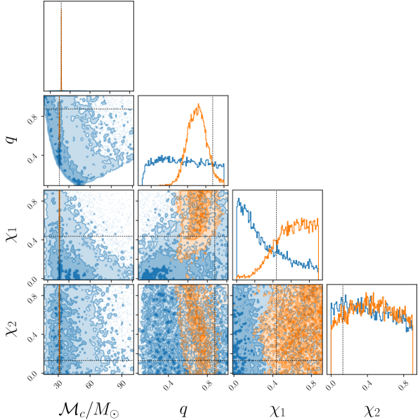
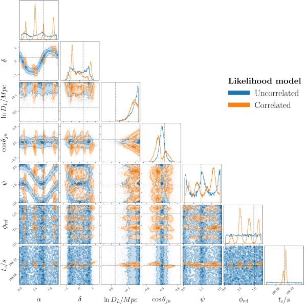
Figure 3: Posterior distributions for the intrinsic (left) and extrinsic parameters (right) of the simulated BBH signal. Contours in the 2D plots enclose the 10%, 50% and 90% of the probability mass. The dashed lines represent the injected values.

References

- Abbott et al. [2016] Abbott, B. P., Abbott, R., Abbott, T. D., et al. 2016, Phys. Rev. Lett., 116, 061102, doi: 10.1103/PhysRevLett.116.061102
- Abbott et al. [2017a] —. 2017a, Phys. Rev. Lett., 119, 141101, doi: 10.1103/PhysRevLett.119.141101
- Abbott et al. [2017b] —. 2017b, Phys. Rev. Lett., 119, 161101, doi: 10.1103/PhysRevLett.119.161101
- Abbott et al. [2020] Abbott, R., Abbott, T. D., Abraham, S., et al. 2020, Phys. Rev. Lett., 125, 101102, doi: 10.1103/PhysRevLett.125.101102
- Abbott et al. [2023] Abbott, R., Abbott, T. D., Acernese, F., et al. 2023, Phys. Rev. X, 13, 041039, doi: 10.1103/PhysRevX.13.041039
- Amaro-Seoane et al. [2023] Amaro-Seoane, P., Andrews, J., Arca Sedda, M., et al. 2023, Living Reviews in Relativity, 26, doi: 10.1007/s41114-022-00041-y
- Badaracco & Harms [2019] Badaracco, F., & Harms, J. 2019, Classical and Quantum Gravity, 36, 145006, doi: 10.1088/1361-6382/ab28c1
- Branchesi et al. [2023] Branchesi, M., Maggiore, M., Alonso, D., et al. 2023, Journal of Cosmology and Astroparticle Physics, 2023, 068, doi: 10.1088/1475-7516/2023/07/068
- Christensen [2018] Christensen, N. 2018, Reports on Progress in Physics, 82, 016903, doi: 10.1088/1361-6633/aae6b5
- Christensen & Meyer [2022] Christensen, N., & Meyer, R. 2022, Rev. Mod. Phys., 94, 025001, doi: 10.1103/RevModPhys.94.025001
- Coughlin et al. [2016] Coughlin, M. W., Christensen, N. L., Rosa, R. D., et al. 2016, Classical and Quantum Gravity, 33, 224003, doi: 10.1088/0264-9381/33/22/224003
- Coughlin et al. [2018] Coughlin, M. W., Cirone, A., Meyers, P., et al. 2018, Phys. Rev. D, 97, 102007, doi: 10.1103/PhysRevD.97.102007
- Davis et al. [2019] Davis, D., Massinger, T., Lundgren, A., et al. 2019, Classical and Quantum Gravity, 36, 055011, doi: 10.1088/1361-6382/ab01c5
- Del Pozzo et al. [2022] Del Pozzo, W., Pagano, G., Carullo, G., & Cireddu, F. 2022, Granite - a software package for gravitational-wave Bayesian parameter estimation, GitHub. https://github.com/wdpozzo/granite
- Driggers et al. [2019] Driggers, J. C., Vitale, S., Lundgren, A. P., et al. 2019, Phys. Rev. D, 99, 042001, doi: 10.1103/PhysRevD.99.042001
- ET steering committee [2020a] ET steering committee. 2020a, Einstein Telescope: Science Case, Design Study and Feasibility Report. https://apps.et-gw.eu/tds/ql/?c=15662
- ET steering committee [2020b] —. 2020b, ET Design Report Update 2020. https://apps.et-gw.eu/tds/ql/?c=15418
- Evans et al. [2021] Evans, M., Adhikari, R. X., Afle, C., et al. 2021, A Horizon Study for Cosmic Explorer: Science, Observatories, and Community. https://arxiv.org/abs/2109.09882
- Gray [2006] Gray, R. M. 2006, Foundations and Trends in Communications and Information Theory, 2, 155, doi: 10.1561/0100000006
- Hild et al. [2011] Hild, S., Abernathy, M., Acernese, F., et al. 2011, Classical and Quantum Gravity, 28, 094013, doi: 10.1088/0264-9381/28/9/094013
- Janssens et al. [2022] Janssens, K., Boileau, G., Christensen, N., Badaracco, F., & van Remortel, N. 2022, Phys. Rev. D, 106, 042008, doi: 10.1103/PhysRevD.106.042008
- Janssens et al. [2021] Janssens, K., Martinovic, K., Christensen, N., Meyers, P. M., & Sakellariadou, M. 2021, Phys. Rev. D, 104, 122006, doi: 10.1103/PhysRevD.104.122006
- Janssens et al. [2023] Janssens, K., Ball, M., Schofield, R. M. S., et al. 2023, Phys. Rev. D, 107, 022004, doi: 10.1103/PhysRevD.107.022004
- Maggiore et al. [2020] Maggiore, M., Broeck, C. V. D., Bartolo, N., et al. 2020, Journal of Cosmology and Astroparticle Physics, 2020, 050, doi: 10.1088/1475-7516/2020/03/050
- Pratten et al. [2021] Pratten, G., García-Quirós, C., Colleoni, M., et al. 2021, Phys. Rev. D, 103, 104056, doi: 10.1103/PhysRevD.103.104056
- Punturo et al. [2010] Punturo, M., Abernathy, M., Acernese, F., et al. 2010, Classical and Quantum Gravity, 27, 194002, doi: 10.1088/0264-9381/27/19/194002
- Thrane et al. [2013] Thrane, E., Christensen, N., & Schofield, R. M. S. 2013, Phys. Rev. D, 87, 123009, doi: 10.1103/PhysRevD.87.123009
- Veitch & Vecchio [2010] Veitch, J., & Vecchio, A. 2010, Phys. Rev. D, 81, 062003, doi: 10.1103/PhysRevD.81.062003