Gain enhanced metal nanoshells: below and above the emission threshold

Abstract

Nanotechnology has revolutionized our ability to control matter at the nanoscale, with metallic nanostructures offering remarkable versatility. Metallic nanoparticles (MNs) find compelling applications when metal losses are balanced by optical gain elements, including visible-frequency metamaterial cloaking and sensitive bio-molecular sensors. Prior studies of the electromagnetic response of these nano-systems have focused on single spherical MNs within infinite gain media, facing non-uniformity challenges beyond emission thresholds. To overcome this issue, we propose transitioning to spherical nanoshells incorporating gain elements, facilitating field homogeneity and offering a comprehensive spectral description using a hybrid quasi-static model. This system enables us to describe the electromagnetic behavior of the MN below as well as above the emission threshold. Interestingly, we found that the steady-state emission of a gain enhanced nanoshell is not the single line emission predicted by other authors, but instead it involves a range of frequencies whose span is governed by physical and morphological parameters that can be chosen at the stage of synthesis to design an optimal emitter.

I Introduction

In the rapidly evolving landscape of scientific discovery, nanotechnology has emerged as a revolutionary field, promising unprecedented control over matter at the nanoscale. Within this scope, metallic nanostructures are particularly interesting as they open up endless application possibilities. To give some examples, metallic nanoparticles (MNs) can be used as catalysts in chemical reactions [1], as contrast agents in medical imaging techniques [2], as carriers for drug delivery [3], and can be integrated into electronic devices, contributing to advancements in miniaturization, energy storage, and the development of flexible and stretchable electronics [4]. Moreover, a new pathway opens up when metal losses are balanced out with optical gain elements pumped with an external field. Applications for these gain-assisted MNs include the potential for creating metamaterial-based cloaking devices operating at visible frequencies  [5, 6, 7], enhancing nano-sensors for detecting drugs and diseases [8], enabling ultra-sensitive bio-molecular sensors [9], and even facilitating the development of plasmon lasers [10], among others. What is more, when metal losses are not only compensated but outgrown by the external pump, a phenomenon called SPASER takes place, and consists on emission coming from the MN in the local field  [11, 12, 13, 14]. If we add an external field to this system, it undergoes an amplification effect.

In previous works, we have studied SPASER and amplification effects on the simplest system possible: a single spherical metal nanoparticle, much smaller than the wavelength of the resonant optical field, immersed in an infinite gain medium  [15, 16]. However, this system configuration led to a phenomenon of non-uniformity of the amplified field, similar to the Spatial Hole Burning phenomenon in Laser Physics, when the gain considered exceeded the emission threshold. This non-uniformity, stemming from the energy transferred from the pump through the gain medium, led to non-uniform consumption in the population inversion of the gain medium and, consequently, non-uniform field amplification, resulting in a cascade of undesirable modes. To address this problem, we propose transitioning from a spherical metal nanoparticle surrounded by a gain medium to a spherical nanoshell incorporating gain elements in its core (see figure 1). In this configuration, especially in the quasi-static limit (where the size of the nanoshell is much smaller than the resonant plasmon frequency), the field in the core becomes homogeneous, as does the depletion of population inversion in the gain medium.

In this paper, we present a hybrid (quantum and classical), quasi-static model that utilizes dynamic constitutive equations, similar to those introduced in former works  [16]. However, in this model, these equations are coupled through boundary conditions specific to the spherical nanoshell geometry. This approach leverages the field’s uniformity in the gain region to provide a comprehensive spectral description of the electromagnetic response of these systems, even beyond the emission threshold.

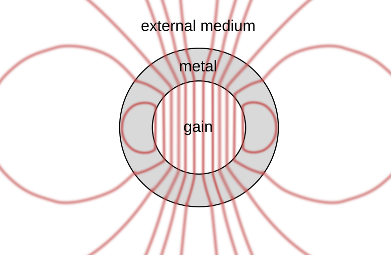
Figure 1: A spherical nanoshell particle, with a gain medium filling the core and a metallic shell, placed into an external medium.

II Dynamical equations for materials

To ensure that our model is able to capture spatial and temporal variations of the fields, our first step is to formulate dynamical constitutive equations for the materials comprised in the nanoshell, i.e., for the metal and the gain medium. This formalism has been described in [16], and the interested reader is referred to the Supplementary Material for detailed derivations [17].

The electron gas in the metal is classically modelled using the free-electron equation of motion [16, 17], with a collision rate $\gamma$ and and a plasma frequency $\omega_{\text{pl}}$. The gain medium is described as a continuum composed of a background host material inside which gain elements (emitters), like dye molecules or quantum dots, are dispersed randomly. The internal dynamics of the emitters is described with the help of an effective two-level approach, which is a phenomenological reduction capturing the essentials of more complete, multiple-level dynamics commonly used in laser physics. We label as levels 1 and 2 the lower and upper states of the resonant transition in the emitters, and call $\omega_{12}$ the angular frequency associated to this transition: $\omega_{12}=(E_{2}-E_{1})/\hbar$. The emitters are provided with energy by some optical pumping process, which details are left out: it is just assumed that the emitters are pumped with some tunable, effective pump rate, at a frequency far from all phenomena of interest. The population dynamics of this gain medium is then obtained with the help of the optical Bloch equations and the matrix density formalism [16, 17].

Denoting $\mathbf{r}$ and $t$ as the spatial and time coordinates, the polarization ${\bf P}_{m}$ in the metal and ${\bf P}_{g}$ in the gain medium can be written as the sum of two contributions:

$${\bf P}_{g}(\mathbf{r},t)=\varepsilon_{0}\chi_{b}{\bf E}_{g}(\mathbf{r},t)+{\bf\Pi}_{g}(\mathbf{r},t),$$ (1)

$${\bf P}_{m}(\mathbf{r},t)=\varepsilon_{0}\chi_{\infty}{\bf E}_{m}(\mathbf{r},t)+{\bf\Pi}_{m}(\mathbf{r},t).$$ (2)

Here, $\varepsilon_{0}$ is the vacuum permittivity, $\chi_{b}$ is the background, passive linear susceptibility of the host medium in which the gain elements are dispersed, and $\chi_{\infty}$ is the background, passive susceptibility of the ion lattice in the metal.

The additional term ${\bf\Pi}_{g}$ accounts for the dipole moments of the emitters within the host medium, and can be explicitly related to the transition dipole moment $\bm{\mu}$ between the two levels as

$${\bf\Pi}_{g}(\mathbf{r},t)=\frac{n}{4\pi}\int_{0}^{\pi}\int_{0}^{2\pi}2\rho_{12}{\bm{\mu}}\sin\theta d\theta d\varphi,$$ (3)

where $n$ is the volumetric concentration of gain elements, $\rho_{12}$ is the element of the density matrix between levels 1 and 2, representing the gain element probability of transition, while $\theta$ and $\varphi$ are respectively the polar and the azimutal angle. The other additional term ${\bf\Pi}_{m}$ is the contribution to polarization due to the free electrons in the metal which is defined as

$${\bf\Pi}_{m}(\mathbf{r},t)=n_{e}e{\bf d},$$ (4)

where $n_{e}$ and $e$ are respectively the electron density and the electron charge, and ${\bf d}$ is the displacement of the electron cloud with respect to the ionic lattice in the free-electron model.

We assume a harmonic form $e^{-i\omega t}$ (where $\omega$ is the angular frequency) for all time-dependent quantities. All calculations in this work will be performed in the rotating waves approximation, i.e., we assume the frequency $\omega$ to stay close to the frequency of the emitter’s transition $\omega_{12}$, and keep track of slow temporal variations only. Therefore, from now on, all fields and polarizations have to be considered complex amplitudes $\stackrel{{\scriptstyle\rule{2.71246pt}{0.0pt}\sim}}{{\smash{\bm{\mathcal{A}}}\rule{0.0pt}{6.02773pt}}}\hskip-2.58334pt(\mathbf{r},t)$ varying on a time scale much larger than $1/\omega$, and related to the real physical values $\bm{\mathcal{A}}(\mathbf{r},t)$ through the formula:

$${\bm{\mathcal{A}}}(\mathbf{r},t)=\frac{1}{2}\left[\stackrel{{\scriptstyle\rule{2.71246pt}{0.0pt}\sim}}{{\smash{\bm{\mathcal{A}}}\rule{0.0pt}{6.02773pt}}}\hskip-2.58334pt(\mathbf{r},t)e^{-i\omega t}+\stackrel{{\scriptstyle\rule{2.71246pt}{0.0pt}\sim}}{{\smash{\bm{\mathcal{A}}}\rule{0.0pt}{6.02773pt}}}\hskip-2.58334pt^{*}\hskip-1.07639pt(\mathbf{r},t)e^{i\omega t}\right]$$ (5)

For convenience, tildas and the dependence in $(\mathbf{r},t)$ of all fields will be dropped and implicitly assumed in equations further down.

One finally obtains the following set of differential equations describing the two material’s time evolution [17]:

$$\frac{d{\bf\Pi}_{g}}{dt}-\left[i(\omega-\omega_{21})-\frac{1}{\tau_{2}}\right]{\bf\Pi}_{g}=-\frac{i\varepsilon_{0}G}{\tau_{2}}\frac{N}{\tilde{N}}{\bf E}_{g},$$ (6)

$$\frac{dN}{dt}+\frac{N-\tilde{N}}{\tau_{1}}=-\frac{i}{2n\hbar}({\bf\Pi}_{g}\cdot{\bf E}^{*}_{g}-{\bf\Pi}_{g}^{*}\cdot{\bf E}_{g}),$$ (7)

$$\frac{d{\bf\Pi}_{m}}{dt}-\frac{\omega(\omega+2i\gamma)}{2(\gamma-i\omega)}{\bf\Pi}_{m}=\frac{\varepsilon_{0}\omega_{\text{pl}}^{2}}{2(\gamma-i\omega)}{\bf E}_{m};$$ (8)

In the above, $N=\rho_{22}-\rho_{11}$ is the space and time-dependent population inversion of the emitters, defined from the difference of the diagonal terms of the density matrix. The time constant $\tau_{2}$ is associated with the effective phase relaxation processes of the emitters, $\tau_{1}$ is the energy relaxation time, and $\tilde{N}$ is the maximal, asymptotic value that the population inversion can reach given the applied pumping rate and spontaneous emission processes (in the absence of any saturation/depletion).

Finally, the quantity $G$ in Eq. 6 will play a pivotal role in the following study, as it represents the overall quantity of gain brought into the system. It is defined as [18]

$$G=\frac{\tau_{2}\mu^{2}}{3\hbar\varepsilon_{0}}n\tilde{N}.$$ (9)

In Ref. [16] about nanolasers made of plasmonic homogeneous spheres and in Ref. [18] about core-shell and nanoshell nanolasers, we discussed the existence of a threshold value $G_{\text{th}}$, dependent on the physical properties of the gain elements and the system’s geometry, such that When $G$ exceeds $G_{\text{th}}$, the systems would transition into an lasing/spasing regime. In the case of the nanoshell geometry, the threshold gain was defined as the point when the classical formula quasi-static polarizability of the particle would become singular. We shall demonstrate in the following that this intuitive definition holds true in the more elaborate model under study in the present work.

The inclusion of the saturation equation (Eq. 7), governing the temporal changes in the population inversion $N$, renders the system of equations (Eqs. 6-8) applicable to various situations that demand dynamic constitutive equations for both the metal and the gain medium. Its solutions encompass, in principle, all possible transient states both above and below the emission threshold, as well as steady states.

Before moving to the case of nanoshells, let us quickly review such steady-state solutions obtained in the case of infinite media subject to uniform electric fields. From equation 8, one can retrieve the standard Lorentz-Drude formula for the permittivity of the metal (see Supplementary Materials [17]):

$$\varepsilon_{m}=\varepsilon_{\infty}-\frac{\omega_{\text{pl}}^{2}}{\omega(\omega+2i\gamma)},$$ (10)

with $\varepsilon_{\infty}=1+\chi_{\infty}$.

For the gain medium modeled by equation 6 along with equation 7, one finds the steady-state permittivity [17]:

$$\varepsilon_{g}=\varepsilon_{b}+\frac{[2(\omega-\omega_{21})-i\Delta]G\Delta}{4(\omega-\omega_{21})^{2}+\Delta^{2}\left[1+\dfrac{\left|\mathbf{E}_{g}\right|^{2}}{{E_{\text{sat}}}^{2}}\right]},$$ (11)

where we defined $\varepsilon_{b}=1+\chi_{b}$, $\Delta=2/\tau_{2}$, and

$$E_{\text{sat}}=\frac{\hbar}{\mu}\sqrt{\frac{3}{\tau_{1}\tau_{2}}}.$$ (12)

Equation 11 stands as a non-linear permittivity for the gain medium, dependent on the modulus of the electric field $\left|\mathbf{E}_{g}\right|$ inside it. This is classically known as a “gain saturation” effect due to the depletion term ${\bf\Pi}_{g}\cdot{\bf E}^{*}_{g}-{\bf\Pi}_{g}^{*}\cdot{\bf E}_{g}$ in eq. 7: when the field in the gain medium becomes large enough, the upper state of the resonant transition of the emitters becomes depleted, causing $N$ to decrease and saturate at some value lower than the maximum allowable value $\tilde{N}$. The typical magnitude of the field where this becomes significant is $E_{\text{sat}}$. In the “small-signal” regime where fields keep small enough, so that $\left|\mathbf{E}_{g}\right|^{2}\ll{E_{\text{sat}}}^{2}$, the above permittivity becomes linear:

$$\varepsilon_{g}=\varepsilon_{b}+\frac{G\Delta}{2(\omega-\omega_{21})+i\Delta},$$ (13)

which is the classical Lorentzian curve used for unsaturated gain media, centered at $\omega=\omega_{12}$, with an emission linewidth $\Delta$.

In the context of nanolasers, however, it must be strongly emphasized that these steady-state permittivities for metal and gain have to be used with outmost care, especially above the threshold of lasing. While expressions 10, 11 and 13 have been widely put to use in the literature to compute the properties of various types of nanolasers, there is in fact no guarantee at all that the long-term state reached by the lasing system will correspond to such a steady state. Our results will indeed show that the lasing regime of the nanoshell cannot be properly computed using the above steady-state permittivites.

III Nanoshell Geometry

We now proceed to specify the geometry of the nanoshell shown in Figure 1, of external radius $r_{\text{ext}}=a$, internal radius $r_{\text{int}}=\rho a$ and aspect ratio $\rho=r_{\text{int}}/r_{\text{ext}}$. The core is filled with the gain medium described in the previous section (eqs. 6-7), and is surrounded by a shell made with the metal described by eq. 8. The whole nanoparticle bathes in a passive, dielectric solvent, with a real, positive permittivity $\varepsilon_{s}$.

We place ourselves in the quasi-static limit, where the nanoparticle’s size is much smaller than the impinging wavelength. The exciting probe field can be approximated as uniform and written as $\tilde{\bf E}_{0}e^{-i\omega t}$, where $\tilde{\bf E}_{0}$ does not depend on spatial position. Within the same approximation, we can introduce the time and space-dependent potentials $\phi_{g,m,s}$ and $\psi_{g,s}$, respectively located in the gain core ($g$), metal shell ($m$) and solvent ($s$), from which the fields and polarizations are derived as ${\bf E}_{g,m,s}=-\nabla\phi_{g,m,s}$ and ${\bf\Pi}_{g,m}=-\nabla\psi_{g,m}$. They must satisfy the Laplace equations:

$$\nabla^{2}\phi_{g,m,s}=0$$ (14)

$$\nabla^{2}\psi_{g,m}=0$$ (15)

It is worth mentioning that in a previous work [19], we established the validity of the relation ${\bf\Pi}_{g,m}=-\nabla\psi_{g,m}$ under the condition that $\nabla\times{\bf\Pi}_{g,m}=0$. In the same paper we discussed how this condition holds true as long as $\nabla N=0$. Notably, in the geometry employed in this paper, this last is always satisfied since the gain is confined to the spherical core of the nanoshell (region 1). All the electrodynamic physical quantities in this region (i. e. electric fields, polarizations, and the relative potentials) are bound to remain homogeneous in the whole parameter space of the problem. This homogeneity is inherited by the left term of equation 7 meaning that if $N$ is homogeneous (e. g. $N=0$ everywhere in the core) at $t=0$, equation 7 cannot drive any spatial dependency on $N(t)$ throughout the whole time evolution.

This is a key consideration to understand why the quasi-static nanoshell configuration is the perfect model system to study the transition from absorption to emission in gain-assisted plasmonic devices. In fact, differently from any other geometry, it allows to ensure that the system will never fall out of the assumptions needed by our model, while being also unable to sustain the Spatial Hole Burning mode cascade who haunts all the other configurations as soon as they shift to emission.

When solved in azimuthal symmetrical systems, using spherical coordinates centered on the NP, equations 14 and 15 produce solutions that can be expressed as a superposition of Legendre Polynomials. Taking into account that the potentials should be regular at $r=0$ and that for $r\gg 1$, the electric field has to reconnect to the external field $\tilde{\bf E}_{0}$ which decides the direction of the $z$-axis (i. e. $\tilde{\bf E}_{0}=E_{0}\hat{\bf z}$), the following expressions for $\phi_{g,m,s}$ and $\psi_{g,m}$ are obtained:

$$\phi_{g}(r,\theta,t) =p_{0}r\cos\theta,$$ (16)

$$\phi_{m}(r,\theta,t) =p_{1}r\cos\theta+\rho^{3}p_{2}\frac{\cos\theta}{r^{2}},$$ (17)

$$\phi_{s}(r,\theta,t) =-E_{0}r\cos\theta+p_{3}\frac{\cos\theta}{r^{2}},$$ (18)

$$\psi_{g}(r,\theta,t) =q_{0}r\cos\theta,$$ (19)

$$\psi_{m}(r,\theta,t) =q_{1}r\cos\theta+\rho^{3}q_{2}\frac{\cos\theta}{r^{2}}.$$ (20)

Coefficients $p_{0}$, $p_{1}$, $p_{2}$, and $p_{3}$ can be computed by enforcing continuity of the fields at the boundaries $r=a$ and $r=\rho a$, with the help of definitions 1 and 2. This procedure yields the following results:

$$p_{3}= \frac{-\varepsilon_{\infty}p_{1}+2\varepsilon_{\infty}\rho^{3}p_{2}-q_{1}+2\rho^{3}q_{2}-\varepsilon_{s}E_{0}}{2\varepsilon_{s}}$$ (21)

$$p_{2}= \frac{\left(\varepsilon_{b}-\varepsilon_{\infty}\right)\left(p_{3}-E_{0}\right)+q_{0}-q_{1}+2q_{2}}{-2\varepsilon_{\infty}-\varepsilon_{b}+\rho^{3}\left(\varepsilon_{b}-\varepsilon_{\infty}\right)}$$ (22)

$$p_{1}= p_{3}-\rho^{3}p_{2}-E_{0}$$ (23)

$$p_{0}= p_{1}+p_{2}.$$ (24)

A detailed calculation of equations 21 to 24 can be found in the Supplementary Material.

We can now use $\phi_{g,m,n}$ and $\psi_{g,m}$ to recalculate the fields and polarizations that have to be substituted in equations 6 and 8. Through this procedure, one will produce a system of equations determining the time evolution of the coefficients $q_{0,1,2}$:

$$\frac{dq_{0}}{dt}-\Omega_{H}q_{0}=\tilde{G}Np_{0}\,;$$ (25)

$$\frac{dq_{1}}{dt}-\Omega_{P}q_{1}=\Gamma_{P}p_{1}\,;$$ (26)

$$\frac{dq_{2}}{dt}-\Omega_{P}q_{2}=\Gamma_{P}p_{2}\,;$$ (27)

where the time evolution population inversion $N$ in equation 25 is determined by:

$$\frac{dN}{dt}+\frac{N-\tilde{N}}{\tau_{1}}=\frac{\Im\left\{q_{0}p_{0}^{*}\right\}}{n\hbar}\,,$$ (28)

which is obtained from equation 7 with the same procedure. In system 25-27 we have also defined:

$$\Omega_{H}=i(\omega-\omega_{21})-\frac{1}{\tau_{2}}$$ (29)

$$\tilde{G}=-\frac{i\varepsilon_{0}G}{\tilde{N}\tau_{2}}$$ (30)

$$\Omega_{P}=\frac{\omega(\omega+2i\gamma)}{2(\gamma-i\omega)}$$ (31)

$$\Gamma_{P}=\frac{\varepsilon_{0}\omega_{\text{pl}}^{2}}{2(\gamma-i\omega)}.$$ (32)

System 25-28 allows to fully describe the electrodynamical behavior of the nanoshell. As evidence of the solidity of this model, one can use it to calculate the steady state solutions for quantities $q_{0}$, $q_{1}$ and $q_{2}$; substitute them into 21 and find that the normalized polarizability $\alpha/(4\pi\varepsilon_{s}a^{3})=p_{3}/E_{0}$ converges to the classical steady-state formula:

$$\frac{(\varepsilon_{m}-\varepsilon_{s})(\varepsilon_{g}+2\varepsilon_{m})+\rho^{3}(\varepsilon_{g}-\varepsilon_{m})(\varepsilon_{s}+2\varepsilon_{m})}{(\varepsilon_{m}+2\varepsilon_{s})(\varepsilon_{g}+2\varepsilon_{m})+2\rho^{3}(\varepsilon_{m}-\varepsilon_{s})(\varepsilon_{g}-\varepsilon_{m})},$$ (33)

here $\varepsilon_{m}$ is defined by expression 10 while $\varepsilon_{g}$ could be defined by expression 13 or 11 depending if the left term of equation 28 is neglected or not.

This result couples with what we discussed in the previous section about the permittivities of the materials. It means that as long as steady-state

$$\frac{dq_{i}}{dt}=0\qquad\text{for }i=0,1,2$$ (34)

can be reached, the use the equation 33 for the polarizability of a nanoshell, including the appropriate steady state formula for the permittivities of metal and dielectric is perfectly legit even when gain is added to the system.

However, in the following we will show that condition 34 breaks when $G\geq G_{\text{th}}$ which is when the nanoparticle enters its emissive regime and a richer phenomenology arise. Nevertheless, even when the emissive regime is reached, the homogeneity of the field in the nanoshell’s core gives us the tactical advantage of preventing any Spatial Hole Burning mode-cascade, this way allowing to find complete numerical solutions for system 25-28.

IV The System Geometry Matrix

Relations 21-24 represent a linear system whose solutions for $p_{0}$, $p_{1}$, $p_{2}$ and $p_{3}$ are linear combinations of $q_{0}$, $q_{1}$, $q_{2}$ and $E_{0}$, namely:

$$p_{0}= p_{00}q_{0}+p_{01}q_{1}+p_{02}q_{2}+p_{03}E_{0},$$ (35)

$$p_{1}= p_{10}q_{0}+p_{11}q_{1}+p_{12}q_{2}+p_{13}E_{0},$$ (36)

$$p_{2}= p_{20}q_{0}+p_{21}q_{1}+p_{22}q_{2}+p_{23}E_{0},$$ (37)

$$p_{3}= p_{30}q_{0}+p_{31}q_{1}+p_{32}q_{2}+p_{33}E_{0}.$$ (38)

We can use the coefficients $p_{ij}$ to define the matrix $\bf A$:

$${\bf A}=\begin{bmatrix}\tilde{G}Np_{00}+\Omega_{H}&\tilde{G}Np_{01}&\tilde{G}Np_{02}\\ \Gamma_{P}p_{10}&\Omega_{P}+\Gamma_{P}p_{11}&\Gamma_{P}p_{12}\\ \Gamma_{P}p_{20}&\Gamma_{P}p_{21}&\Omega_{P}+\Gamma_{P}p_{22}:\end{bmatrix},$$ (39)

and the vector $\bf{b}$:

$${\bf b}=(\tilde{G}p_{03},\Gamma_{P}p_{13},\Gamma_{P}p_{23})E_{0}.$$ (40)

Using $\bf{A}$ and $\bf{b}$ and reorganizing the coefficients $q_{i}$ in the vector $\tilde{\bf q}$:

$$\tilde{\bf q}=(q_{0},q_{1},q_{2}),$$ (41)

system of equations 25-27 can be rewritten in the form:

$$\frac{d\tilde{\bf q}}{dt}={\bf A}\tilde{\bf q}+{\bf b},$$ (42)

$$\frac{dN}{dt}+\frac{N-\tilde{N}}{\tau_{1}}=\frac{\Im\left\{q_{0}p_{0}^{*}\right\}}{n\hbar}.$$ (43)

In this section, we have constructed a robust, time-dependent model represented by equations 42-43. This model seamlessly integrates with the well-established formulas for polarizability and material permittivity commonly employed to describe a nanoshell in steady-state plasmonics, provided that condition 34 is satisfied.

In the next section, we will numerically solve this model as we investigate the case of a silver nanoshell containing a silica core and immersed in water. Our aim is to uncover the electrodynamic behavior of this structure when it is pumped above the gain threshold $G_{\text{th}}$.

V A gain enhanced silver nanoshell

Since the importance of studying this topic lies in the applications, it is fundamental to put our model to the test on a realistic example. We choose to consider a silver nanoshell of external radius $a_{2}=10$ nm, with a radius ratio $\rho=0.6$, including a gain enhanced silica core and dissolved in water. To take into account the last two materials we just need to set $\varepsilon_{b}=2.1316$ and $\varepsilon_{s}=1.7689$; in order to describe silver we have used $\hbar\omega_{\text{pl}}=9.6$ eV and $\hbar\gamma=0.0228$ eV. For the gain elements we have set $\hbar\Delta=0.15$ eV thus setting $\tau_{2}$ accordingly and $\tau_{1}=5\tau_{2}$.

Next, we follow the procedure outlined in a previous work [18] to calculate the singular resonance frequency $\omega_{\text{sp}}$ and the gain threshold $G_{\text{th}}$ when the gain emission center-line coincides with the plasmon resonance frequency, (i. e. $\omega_{21}=\omega_{\text{sp}}$). For the specific system we describe, this results in $\omega_{\text{sp}}=2.812972$ eV and $G_{\text{th}}=0.1349066$. It’s important to note that the system exhibits high sensitivity around these thresholds, necessitating the presentation of their numerical values with up to seven decimal places. Finally the amplitude of the probe field $E_{0}\sim 10^{-9}E_{\text{sat}}$ was chosen to ensure that the system is in the small signal regime.

It’s important to highlight that when the field in the core remains sufficiently small, the left term of equation 43 becomes negligible, and the population inversion $N$ converges to $\tilde{N}$ in a time period approximately on the order of $\tau_{1}$. Under these conditions, the system described by Equation 42 can be effectively solved analytically. This analytical solution remains accurate until the system reaches the emission state.

VI Time dynamics

The solutions ${\bf q}(t)$ for the system of equations 42-43 exhibit inherent time dependence, which is influenced by the selected initial condition. In all our calculations, we adopted a non-excited system as the initial condition (i. e. ${\bf q}(0)=(0,0,0)$), where $t=0$ corresponds to the moment when the exciting probe field $\tilde{\bf E}_{0}$ is activated.

In the following sections, we will explore the dynamic behavior of this system both below and above the emission threshold. It’s crucial to emphasize that, owing to the resonant nature of these systems, the time evolution of this parameter exhibits significant dependence on the selected frequency, for this reason we calculated this time-behavior for $\omega=2.811$ eV, which is in proximity to, but not precisely equal to, the singular resonance frequency $\omega_{\text{sp}}$.

Below the Emission Threshold — We initiated our calculations with the pump switched off. As illustrated in figure 2, the solutions for $q_{0}$, $q_{1}$ and $q_{2}$ swiftly approaches a non-pumped steady state within a few picoseconds. At $t=10$ ps, upon activating the pump (i. e. setting a $G$ value higher than zero), the system subsequently achieves its pumped steady state (again in under $10$ ps).

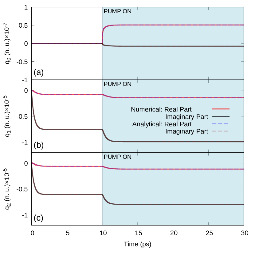
Figure 2: Analytical and Numerical solutions calculated for $\hbar\omega=2.811$ eV with a sub-emissive gain quantity ($G=0.033$). The pump is switched on at $t=10$ ps. We present the real and imaginary part of: (a) $q_{0}$; (b) $q_{1}$; (c) $q_{2}$. The numerical solutions are presented in continuous lines (red and black respectively for the real and imaginary part) while the analytical solutions are presented in dashed lines (purple and brown respectively for the real and imaginary part).

It is evident here that the value of $q_{0}$ is two orders of magnitude smaller than $q_{1}$ and $q_{2}$, signifying that the dynamic component of the polarization in the gain-enriched silica core is significantly smaller than its counterpart in the silver shell.

It’s essential to observe that in this regime, the analytical and numerical solutions perfectly overlap. This is attributable to the fact that the field intensity in the gain-rich region remains sufficiently low, preventing the activation of the saturation term (which cannot be accounted by the linear analytical solution).

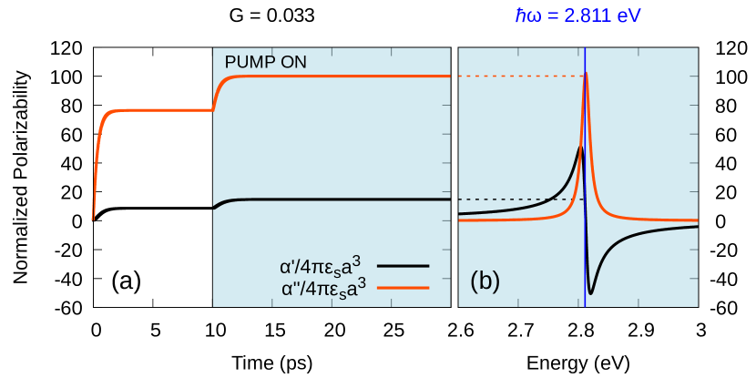
Figure 3: Normalized polarizability with a sub-emissive gain quantity ($G=0.033$). The real and imaginary parts are shown as black and orange lines, respectively. (a) Time dependence calculated for $\hbar\omega=2.811$ eV. (b) Steady-state spectrum. A blue line at $\hbar\omega=2.811$ eV serves as a reference.

To validate the solutions presented in Figure 2, we should note that when these solutions are substituted into Equation 38 (or Equation 21), they allow for the calculation of a time-dependent polarizability, denoted as $\alpha(t)/(4\pi\varepsilon_{s}a^{3})$ and defined as $p_{3}(t)/E_{0}$. The time evolution of this quantity is depicted in Figure 3(a), where it can be compared with the spectrum of the pumped steady state of the same quantity calculated using equation 33 and presented in figure 3(b). To facilitate the comparison, the frequency used for the calculation of the time evolution is indicated by a vertical blue line. The time-dependent polarizability rapidly converges to the steady state calculated using the well-known steady-state formula. This indicates that, below the emission threshold (and in the small-signal regime), it is entirely legitimate to model the effect of gain by substituting expression 13 into the steady-state formula for polarizability.

Above the Emission Threshold — The situation undergoes a dramatic transformation with even a slight increase in the added gain above the threshold $G_{\text{th}}$.

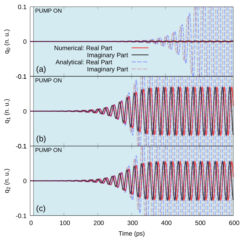
Figure 4: Analytical and Numerical solutions at $\hbar\omega=2.811$ eV with a super-emissive gain quantity ($G\sim 0.136$). The pump is switched on at $t=10$ ps. Time evolution for the real and imaginary part of: (a) $q_{0}$; (b) $q_{1}$; (c) $q_{2}$. The numerical solutions are presented in continuous lines (red and black respectively for the real and imaginary part) while the analytical solutions are presented in dashed lines (purple and brown respectively for the real and imaginary part).

In the calculation shown in Figure 4, for instance, we employed a gain value of just $1.01G_{\text{th}}$, yet the resulting amplification is orders of magnitude greater. It’s also worth noting that the time required for the system to reach saturation is significantly longer than the typical times needed in the sub-emissive scenario to converge to a steady state. This is associated with the parameters we have chosen, particularly the intentionally small amplitude $E_{0}$ of the exciting field, which has been selected to maintain the system within the small-signal regime. In the set of variables employed for the calculation presented in figure 4, saturation takes place between $250$ and $300$ picoseconds. This also marks the time at which the numerical solution of the system (considering saturation) diverges from the analytical solution (which disregards saturation). This is the time limit beyond which non-saturated time-dynamic models, such as the ones we presented in [15] and [19], cease to be effective.

It’s important to note that neither the analytical nor the numerical solutions reach a true steady state; they appear to continue oscillating at a fixed frequency indefinitely. This implies that when solved for a quantity of gain above the emission threshold, the solution of system 42 (after an initial transient) assumes the following form:

$$\tilde{\bf q}(t)=\tilde{\bf Q}e^{i\Omega t},$$ (44)

Where $\tilde{\bf Q}$ is a constant, complex vector amplitude and $\Omega$ the oscillation frequency. This behavior can be ascribed to the saturation term’s dependence on the field’s intensity in the gain region rather than its amplitude. As a result, it ensures a steady state solely for the intensity of the fields and polarizations, not their amplitudes (We will explore more details of this connection further in the paper). It’s crucial to recall here that $\tilde{\bf q}(t)$ represents already a complex, slowly varying amplitude. Consequently, solutions in this form are physically valid only in the limit where $\Omega\ll\omega$. Through our simulations, we determined $\Omega$ via a Fourier analysis of each of ours numerical solutions. We found that $\Omega$ is a function of the exciting field frequency $\omega$ and that, in our parameters range, it falls within the range of $-0.2$ eV$<\hbar\Omega<0.2$ eV. This implies that the rotating wave approximation introduced in our model is applicable when working in the visible range (i.e., $1.63$ to $3.26$ eV). However, it also suggests that nanoparticles resonating in the infrared may require a different approach.

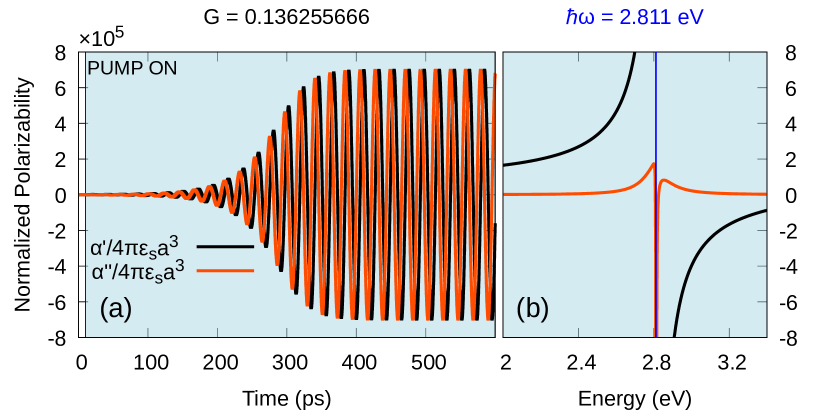
Figure 5: Normalized polarizability with a super-emissive gain quantity ($G\sim 0.136$). The real and imaginary parts are shown as black and orange lines, respectively. (a) Time dependence calculated for $\hbar\omega=2.811$ eV. (b) Steady-state spectrum. A blue line at $\hbar\omega=2.811$ eV serves as a reference.

In figure 5(a), we illustrate the super-emissive behavior of the time-dependent polarizability. Notably, (I) the polarizability as well never seems to reach a true steady state, and (II) its behavior is entirely distinct from the steady state calculated using equation 33 and plotted in figure 5(b) as reference. This implies that above the emission threshold, using expression 13 for the permittivity of the gain medium in the steady-state polarizability, formula 33 is not physically accurate and may produce artifacts.

Intensity and Time Dynamics — To better understand the saturation mechanism, one can observe that equation 25 implies that the amplitude of the solution for $q_{0}$ must, over time, become proportionate to the amplitude of $p_{0}$. Consequently, the source term $\Im\left\{q_{0}p_{0}^{*}\right\}/(n\hbar)$ in equation 28 will eventually become directly proportional to $|p_{0}|^{2}.$ Additionally, from equation 16, it can be easily calculated that the field intensity in the gain-enriched silica core is $|E_{g}|^{2}=|p_{0}|^{2}$. These straightforward considerations illustrate how equation 28 connects the field intensity in the core with the population inversion. In the specific case study we are discussing here, this relationship is visualized in figure 6 (where the field intensity is represented by a green filled-curve and the population inversion by a magenta continuous line).

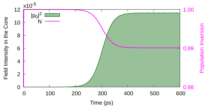
Figure 6: The green filled curve represents the field intensity in the gain-enriched silica core, denoted as $|p_{0}|^{2}$. The continuous magenta line illustrates the population inversion $N$ of the gain elements. Both are calculated at the frequency corresponding to $\hbar\omega=2.811$ eV, and employ a gain quantity $G\sim 0.136$

Here, at $t=10$ (i. e. when the pump is switched on), the field intensity in the core is sufficiently low that the source term $\Im\left\{q_{0}p_{0}^{*}\right\}/(n\hbar)$ is much smaller than $\tau_{1}$, so equation 28 rapidly drives the population inversion $N$ to $\tilde{N}=1$. In the super-emissive regime, this implies that $GN>G_{\text{th}}$, resulting in an exponential growth for $q_{0}$ (see eq. 25 and eq. 30). This growth is then reflected in the field intensity in the core, reaching a point where it renders the term $\Im\left\{q_{0}p_{0}^{*}\right\}/(n\hbar)$ significant, leading to a decrease in population inversion. This behavior continues until $GN<G_{\text{th}}$ (corresponding to $N=0.99$ in our case study), threshold at which the system is shifted out of the exponential growth regime effectively limiting the field amplification.

There are some residual oscillations in the time dynamics of $|p_{0}|^{2}$ (and consequently in that of $N$), which are hardly noticeable within the parameter range utilized in our calculations. This phenomenon would require more extensive investigation and in-depth discussion which is out of the scope of the present paper. However, it is worth mentioning that these oscillations become more pronounced when $G$ is chosen closer to $G_{\text{th}}$ or when the exciting field $\tilde{\bf E}_{0}$ is more intense. Suggesting that they could be a plasmonic analogous to the Rabi Oscillations [20].

VII Emission Spectrum

From equation 18, it is evident that the scattered field takes the form of a dipolar field with a dipole moment ${\bf p}_{3}$ having a magnitude of $p_{3}$ and being oriented along the $z$ axis. Therefore, by conducting calculations across a range of frequencies up to the steady-state intensity, we can characterize the spectral emission behavior of the system by plotting $|{\bf p}_{3}|^{2}$ as a function of frequency.

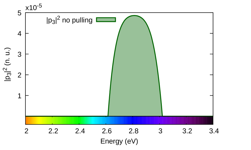
Figure 7: The green filled curve represents the intensity of the scattered dipolar field intensity $|p_{3}|^{2}$ calculated as a function of frequency and using a gain quantity $G\sim 0.136$

The result of this characterization is presented in figure 7, where it is evident that the emission is predominantly confined to a region of the spectrum centered around the plasmon resonance frequency $\omega_{\text{sp}}$. However, the emission band appears unexpectedly wider than expected especially when compared to the spectral region where the imaginary part of the steady-state polarizability is negative (see fig.5(b)). This discrepancy between the two spectral regions is not very plausible because, as we discussed in the past [15, 18], in regions where the imaginary part of the polarizability is positive, the nanoparticle should exhibit its typical absorbing behavior.

Energy Pulling — To settle this apparent conundrum and understand the physical significance of the additional rotation $\Omega$, two pieces of information need to be combined: firstly, as discussed in the previous section, the solutions of system 42-43 converge to the oscillating steady-state introduced in equation 44; secondly, these solutions represent the complex amplitudes of real physical quantities. If one chooses to recalculate these using a formula similar to equation 5, they will obtain a real solution in the form:

$${\bf q}(t)=\frac{1}{2}\left[\tilde{\bf Q}e^{-i(\omega-\Omega)t}+\tilde{\bf Q}e^{i(\omega-\Omega)t}\right].$$ (45)

If we now recall that the real form of the incident probe field is:

$${\bf E}_{0}(t)=\frac{1}{2}\left[\tilde{\bf E}_{0}e^{-i\omega t}+\tilde{\bf E}_{0}e^{i\omega t}\right].$$ (46)

It is evident that an electromagnetic excitation at the frequency $\omega$ will generate a local plasmonic field at the frequency $\omega-\Omega$. As a consequence, in order to visualize correctly the emission spectrum of our system one has to plot $|{\bf p}_{3}|^{2}$ as a function of the shifted frequency $\omega-\Omega$.

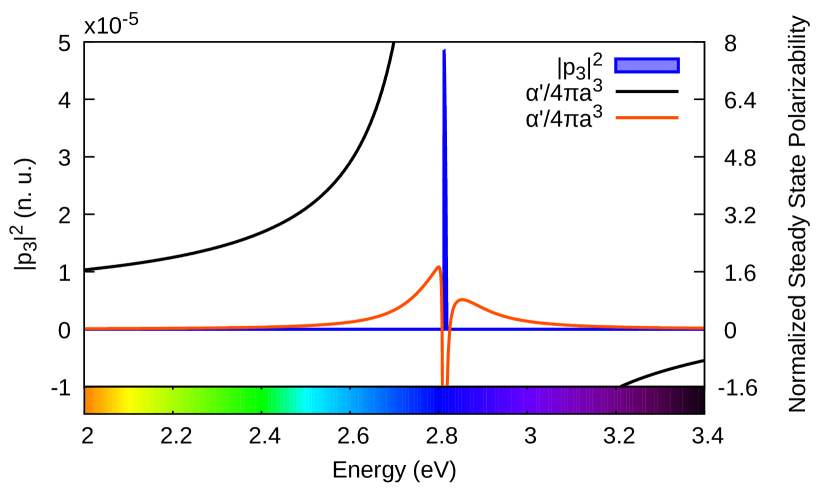
Figure 8: The blue filled curve represents the intensity of the scattered dipolar field intensity $|p_{3}|^{2}$ calculated as a function of frequency, using a gain quantity $G\sim 0.136$ and taking into account the frequency pulling. The steady state normalized polarizability is plotted as a reference

The result of this characterization, as shown in figure 8, highlights a strong energy pulling effect towards the spasing frequency $\omega_{\text{sp}}$, which results in the noticeably narrower emission bandwidth (compared to the one in fig. 7). A consequence of this is that now the emissive region is (as expected) completely included in the spectral region where the imaginary part of the polarizability (presented in fig. 8 as a reference) becomes negative.

This energy pulling effect, represents a completely novel phenomenon, not present in the literature to the best of our knowledge. However, it also holds paramount importance as it fundamentally governs the emissive characteristics of these systems.

VIII Characteristics of the emission spectra

In this section we present some of the possible characterizations our model could allow. All of the results presented in this sections are calculated for the same system described in section V, beside for the physical quantity which we explicitly declare to vary.

In section VII, in order to appreciate the sensibility of the emission threshold, we used a very small amount of gain (i. e. $G=1.01G_{\text{th}}$). Now, it is of interest to delve into the effect of varying gain levels on the quality of the emission line. figure 9(a) illustrates the maximum emission intensity (blue filled curve) and the emission bandwidth (red curve) as functions of the gain level $G$ normalized to the gain threshold $G_{\text{th}}$. As expected, the emission appears when $G/G_{\text{th}}=1$. From that point onward, both the maximum emission intensity and the bandwidth monotonously increase.

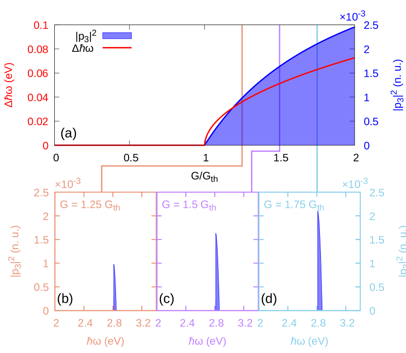
Figure 9: (a): The blue filled curve represents the maximum emission intensity, while the red curve represents the emission bandwidth, both plotted as a function of the quantity of gain. (b) Emission spectrum for $G=1.25G_{\text{th}}$, (c) Emission spectrum for $G=1.5G_{\text{th}}$ (d) Emission spectrum for $G=1.75G_{\text{th}}$

Notably, by increasing the quantity of gain up to $G=2G_{\text{th}}$, a bandwidth of $\Delta\hbar\omega\sim 0.07$ eV is achieved (ranging from $2.81$ to $2.88$ eV and thus corresponding to a line-width of about $11$ nm). Which, while not completely monochromatic, it is still notably narrow. This is probably more evident in figure 9(b-d), where we present the emission spectra corresponding to $G=1.25G_{\text{th}}$, $G=1.5G_{\text{th}}$, and $G=1.75G_{\text{th}}$ respectively. Here, in fact, one can see that aspect ratio of the emission does not change significantly.

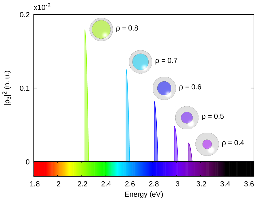
Figure 10: Emission spectra for nanoshells with varying radius ratios $\rho$. For each, the gain quantity was chosen as $G=1.2G_{\text{th}}$

The resonance frequency $\omega_{\text{sp}}$ of a nanoshell is dictated by its radius ratio $\rho$, and this holds true in the emission regime. In Figure 10, we present the emission spectra of different nanoshells with radius ratios ranging from $0.4$ to $0.8$. To ensure a fair comparison, each nanoshell is subjected to a consistent quantity of gain, set at $G=1.2G_{\text{th}}$.

Figure 10 illustrates that varying the radius ratio $\rho$ of a nanoshell can, in principle, produce nano-emitters spanning different colors of the visible spectrum, from green ($\rho=0.8$) to violet ($\rho=0.4$). Additionally, it’s notable that the impact of the gain elements is more pronounced when the metal volume fraction of the nanoshell is smaller. This effect is even more significant than it appears here because we maintained an equal quantity of gain relative to the gain threshold, and the gain threshold itself (affected by metal losses) is larger for nanoparticles with a small radius ratio (indicative of a larger metal volume fraction) [18].

To provide context, it’s worth mentioning that for the $\rho=0.4$ nanoshell, we calculated a $G_{\text{th}}=0.2934669$. Consequently, the applied gain in Figure 10 to produce the violet emission line was $G\sim 0.35$. In contrast, for the $\rho=0.8$ nanoshell, we calculated a $G_{\text{th}}=0.0956313$ meaning that the corresponding applied gain we used to produce the green emission line was $G\sim 0.11$. This means that a $\rho=0.8$ nanoshell delivers an emission line five times more intense than a $\rho=0.4$ nanoshell, achieved with a quantity of gain more than three times smaller.

IX Conclusions

To fully harness the potential of gain-enhanced nanoshells in diverse applications, a comprehensive theoretical grasp of their electromagnetic behavior is essential. Our model not only extends understanding beyond the emission threshold but also provides key insights:

(a) Contrary to expectations, the “singular resonance frequency” $\omega_{\text{sp}}$ is not the only frequency at which the system emits. Emission occurs across a non-monochromatic, albeit narrow, frequency range.

(b) Steady-state formulas, effective below the emission threshold, lose their efficacy once the threshold is surpassed. Notably, the widely used saturation formula (11) encounters obstacles as equations (6) and (7) fail to reach an amplitude steady-state. Consequently, the derivation of that formula is rendered impossible.

(c) Our discovery of the novel energy-pulling effect governs the emissive behavior, offering a fresh perspective on the operational dynamics of these systems.

In terms of future directions, investigating system dynamics with $E_{0}=0$ emerges as a compelling avenue. This exploration provides a unique opportunity to scrutinize the Spaser phenomenon free from external influences. Such studies promise insights into novel aspects, including a deeper understanding of the energy-pulling effect, contributing to a more comprehensive comprehension of the system’s behavior. This line of inquiry holds great potential for unlocking further insights into the intriguing realm of Spasers, potentially paving the way for enhanced control and utilization of these nanostructures across various applications.

Even within the quasi-static limit we used in this work, subtle nuances demand attention. Our analytical dynamical model seamlessly bridges the gap across the emission threshold, offering a continuous and improved understanding of the electrodynamics of gain-enhanced nanoshells, especially in their most intriguing regime. This lays the foundation for additional characterizations, shedding light on the feasibility of these structures as local plasmonic nano-emitters.

References

- Ranu et al. [2009] B. C. Ranu, K. Chattopadhyay, L. Adak, A. Saha, S. Bhadra, R. Dey, and D. Saha, Pure and Applied Chemistry 81, 2337 (2009).
- Siddique and Chow [2020] S. Siddique and J. C. L. Chow, Nanomaterials 10, 1700 (2020).
- Ashfaq et al. [2017] U. Ashfaq, M. Riaz, E. Yasmeen, and M. Z. Yousaf, Crit Rev Ther Drug Carrier Syst. 34, 317 (2017).
- Hales et al. [2020] S. Hales, E. Tokita, R. Neupane, U. Ghosh, B. Elder, D. Wirthlin, and Y. L. King, Nanotechnology 31, 172001 (2020).
- Schurig et al. [2006] D. Schurig, J. J. Mock, B. J. Justice, S. A. Cummer, J. B. P. a. A. F. Starr, and D. R. Smith, Science 314, 977 (2006).
- Cai et al. [2008] W. Cai, U. K. Chettiar, A. V. Kildishev, and V. M. Shalaev, Nature Photon. 1, 224 (2008).
- Veltri [2009] A. Veltri, Optics express 17, 20494 (2009).
- Huang et al. [2017] L. Huang, J. Wan, X. Wei, Y. Liu, J. Huang, S. Xuming, Z. Ru, D. Gurav, V. Sundari, Y. Li, R. Chen, and K. Qian, Nature Communications 8 (2017).
- Tao et al. [2015] Y. Tao, Z. Guo, A. Zhang, J. Zhang, B. Wang, and S. Qu, Optics Communications 349 (2015).
- Yu et al. [2016] M. Yu, J. Song, H. Niu, and J. Qu, Plasmonics 11, 231 (2016).
- Noginov et al. [2009] M. A. Noginov, G. Zhu, A. M. Belgrave, R. Bakker, V. M. Shalaev, E. E. Narimanov, S. Stout, E. Herz, T. Suteewong, and U. Wiesner, Nature 460, 1110 (2009), number: 7259 Publisher: Nature Publishing Group.
- Plum et al. [2009] E. Plum, V. Fedotov, P. Kuo, D. Tsai, and N. Zheludev, Optics Express 17, 8548 (2009).
- Zheludev et al. [2008] N. Zheludev, S. Prosvirnin, N. Papasimakis, and V. Fedotov, Nature Photon. 2, 351 (2008).
- Stockman [2008] M. I. Stockman, Nature Photonics 2, 327 (2008).
- Veltri and Aradian [2012] A. Veltri and A. Aradian, Physical Review B 85, 115429 (2012).
- Veltri et al. [2016] A. Veltri, A. Chipouline, and A. Aradian, Scientific Reports 6, 33018 (2016).
- [17] Supplementary Material available online at: (url to be inserted here by Journal staff).
- Caicedo et al. [2022] K. Caicedo, A. Cathey, M. Infusino, A. Aradian, and A. Veltri, Journal of the Optical Society of America B 39, 107 (2022).
- Recalde et al. [2023] N. Recalde, D. Bustamante, M. Infusino, and A. Veltri, Materials 16, 10.3390/ma16051911 (2023).
- Cohen-Tannoudji et al. [1977] C. Cohen-Tannoudji, B. Diu, and F. Laloë, Quantum mechanics; 1st ed. (Wiley, New York, NY, 1977) trans. of : Mécanique quantique. Paris : Hermann, 1973.