Fidelity Estimation of Entangled Measurements with Local States

Abstract

We propose an efficient protocol to estimate the fidelity of an $n$-qubit entangled measurement device, requiring only qubit state preparations and classical data post-processing. It works by measuring the eigenstates of Pauli operators, which are strategically selected according to their importance weights and collectively contributed by all measurement operators. We rigorously analyze the protocol’s performance and demonstrate that its sample complexity is uniquely determined by the number of Pauli operators possessing non-zero expectation values with respect to the target measurement. Moreover, from a resource-theoretic perspective, we introduce the stabilizer Rényi entropy of quantum measurements as a precise metric to quantify the inherent difficulty of estimating measurement fidelity.

1 Introduction

In recent years, substantial advancements have been made in constructing intermediate-scale quantum devices spanning diverse physical platforms [Pre18, OFV09, KMW02, JVEC00, CWP16]. A pivotal phase in the fabrication of such devices involves assessing the performance of the measurement apparatus. This assessment can be executed through methodologies like measurement (detector) tomography [Fiu01, LFCR⁺09, Hof10, CFYW19], or through measurement fidelity estimation protocols, including those augmented by machine learning [HS10, MC13, LMC⁺19, NOL⁺21], or methods that establish bounds on average measurement fidelity [MC13]. Nevertheless, complete tomography encounters challenges related to high sample complexity, rendering it impractical for large-scale systems. Conversely, measurement fidelity estimation protocols prove significantly more efficient, albeit their potential dependence on entangled state preparation. In scenarios necessitating entangled state preparation, the precision of the estimated fidelity can be notably affected by errors associated with state preparation, particularly in the noisy intermediate-scale quantum (NISQ) era [Pre18].

In this work, we present an efficient protocol for estimating the fidelity of quantum measurement devices, exhibiting an exponential acceleration compared to quantum detector tomography and applicability to diverse quantum measurement schemes. First, we articulate the problem formulation. Consider a system comprising $n$ qubits, represented by a Hilbert space $\mathcal{H}$ with a dimension of $2^{n}$. Our protocol specifically targets the fidelity estimation of a general class of measurements—known as a projection-valued measure (PVM). By showcasing the efficacy of our protocol in certifying a wide range of measurement schemes, including Bell measurements and Elegant Joint Measurement (EJM) [Gis19, TGB21], we affirm its potential to significantly contribute to the advancement of experimental quantum information science.

Our devised protocol operates by conducting measurements on a randomly selected subset of Pauli observables, employing an importance sampling technique [KR21]. Specifically, we calculate the importance weights associated with all ideal PVMs relative to each Pauli operator. Through the accumulation of measurement statistics from this process, we can effectively estimate the measurement fidelity $\mathcal{F}(\mathcal{M},\mathcal{N})$ between the ideal measurement $\mathcal{M}$ and its actual implementation $\mathcal{N}$. The preparation of product eigenstates for each Pauli observable necessitates repeated calls to the measurement device. The number of calls that the protocol makes to measurement device, which we shall call the sample complexity, depends on the specified measurement $\mathcal{M}$ of interest, the desired additive error $\varepsilon$, and the targeted failure probability denoted as $\delta$. We derive analytic bounds on the average sample complexity to elucidate the efficiency of our protocol. We compare our efficient protocol with two other protocols—the globally optimal estimation protocol that involves entangled state preparation and the “direct” measurement fidelity estimation protocol adapted from the seminal direct fidelity estimation proposal by Flammia and Liu [FL11] —and highlight our protocol’s unique advantage in experimental feasibility and efficiency. Furthermore, we conduct comprehensive numerical simulations to substantiate the effectiveness of our protocol.

2 An efficient protocol

2.1 Protocol description

The fidelity between a known ideal $n$-qubit projective measurement $\mathcal{M}$ and its actual implementation $\mathcal{N}$ is defined as

$$\mathcal{F}(\mathcal{M},\mathcal{N}) \mathrel{\mathop{\mathchar 58\relax}}=\frac{1}{2^{n}}\sum_{k=1}^{2^{n}}\operatorname{Tr}[\psi_{k}V_{k}],$$ (1)

where $\mathcal{M}\equiv\{\psi_{k}=\proj{\psi_{k}}\}_{k}$ represents the ideal PVM satisfying $\sum_{k=1}^{2^{n}}\psi_{k}=\operatorname{id}$, where $\operatorname{id}$ is the identity operator, while $\mathcal{N}\equiv\left\{V_{k}\right\}_{k}$ denotes the actual positive operator-valued measure (POVM) satisfying $0\leq V_{k}\leq\operatorname{id}$ and $\sum_{k=1}^{2^{n}}V_{k}=\operatorname{id}$. Note that the specification of $\mathcal{M}$ is known to the experimenters but the specification of $\mathcal{N}$ is completely unknown. The task is to estimate the fidelity $\mathcal{F}(\mathcal{M},\mathcal{N})$ given accesses to $\mathcal{N}$. In the following, we construct an efficient protocol to accomplish this task using local state preparations and rigorously analyze the protocol’s performance.

Expanding the measurement operators $\psi_{k}$ in terms of the set of normalized Pauli operators $\{P_{k}\}_{k},k=1,2,...,4^{n}$, which constitutes an orthonormal basis of the $n$-qubit operators, we obtain

$$\mathcal{F}(\mathcal{M},\mathcal{N})=\frac{1}{2^{n}}\sum_{k=1}^{2^{n}}\operatorname{Tr}\left[\left(\sum_{l=1}^{4^{n}}\operatorname{Tr}[\psi_{k}P_{l}]P_{l}\right)V_{k}\right]=\frac{1}{2^{n}}\sum_{k=1}^{2^{n}}\sum_{l=1}^{4^{n}}\operatorname{Tr}[\psi_{k}P_{l}]\operatorname{Tr}[V_{k}P_{l}].$$ (2)

In order to construct an estimator for $\mathcal{F}(\mathcal{M},\mathcal{N})$, we define a probability mass function $\{q_{l}\}_{l=1}^{4^{n}}$ with respect to the Pauli operators as

$$q_{l} \mathrel{\mathop{\mathchar 58\relax}}=\frac{\sum_{k=1}^{2^{n}}\operatorname{Tr}[\psi_{k}P_{l}]^{2}}{2^{n}}.$$ (3)

Thanks to the property of PVM, we can show that $\sum_{l=1}^{4^{n}}q_{l}=1$ and thus $\{q_{l}\}_{l}$ is a valid probability mass function. Now, we employ the importance sampling technique [KR21] to estimate $\mathcal{F}$ via Eq. (2). To this end, we rewrite $\mathcal{F}$ as

$$\mathcal{F}=\sum_{l=1}^{4^{n}}\left(\sum_{k^{\prime}=1}^{2^{n}}\frac{\operatorname{Tr}[\psi_{k\textquoteright}P_{l}]^{2}}{2^{n}}\right)\times\left(\sum_{k=1}^{2^{n}}\operatorname{Tr}[V_{k}P_{l}]\frac{\operatorname{Tr}[\psi_{k}P_{l}]}{\sum_{k^{\prime}=1}^{2^{n}}\operatorname{Tr}[\psi_{k\textquoteright}P_{l}]^{2}}\right)\equiv\sum_{l=1}^{4^{n}}q_{l}X_{l},$$ (4)

where the random variable $X_{l}$ is defined as

$$X_{l}\mathrel{\mathop{\mathchar 58\relax}}=\frac{\sum_{k=1}^{2^{n}}\operatorname{Tr}[V_{k}P_{l}]\operatorname{Tr}[\psi_{k}P_{l}]}{\sum_{k^{\prime}=1}^{2^{n}}\operatorname{Tr}[\psi_{k\textquoteright}P_{l}]^{2}}.$$ (5)

We can show that $\mathbb{E}[X_{l}]=\mathcal{F}$, where $\mathbb{E}[\cdot]$ denotes the expectation value, signifying that $X_{l}$ serves as an unbiased estimator of $\mathcal{F}$. From Eq. (4), we can construct an estimator of $\mathcal{F}$ using the sample mean in the following manner. Initially, $m$ indices $l_{i}$, where $i=1,2,...,m$ and $l_{i}\in\{1,2,...,4^{n}\}$, are sampled according to the importance sampling distribution $\{q_{l}\}_{l}$ defined in Eq. (3), completely determined by the known ideal PVM $\mathcal{M}$, where

$$m=\left\lceil 1/(\varepsilon^{2}\delta)\right\rceil$$ (6)

and $\lceil\cdot\rceil$ denotes rounding up. Given the estimated values $\{X_{l_{i}}\}_{i=1}^{m}$, whose estimation procedure will be presented below, we can construct an estimator of $\mathcal{F}$ using the following formula:

$$Y=\frac{1}{m}\sum_{i=1}^{m}X_{l_{i}}.$$ (7)

By Chebyshev’s inequality (see Appendix A for detailed arguments), we assert that $Y$ is an $\varepsilon$-accurate estimator of $\mathcal{F}$ satisfying

$${\rm Pr}\left(|Y-\mathcal{F}|\geq\varepsilon\right)\leq\delta,$$ (8)

where $\varepsilon$ and $\delta$ are predefined constant additive error and failure probability, respectively.

It is noteworthy that for each randomly chosen $l$, the quantity $\operatorname{Tr}[V_{k}P_{l}]$ need to be estimated from the measurement statistics in order to determine $X_{l}$. Since $P_{l}$ is not a quantum state, it cannot be used as an input to the measurement device directly. Thanks to the linearity of the trace function, we can consider the spectral decomposition

$$P_{l}=\sum_{a=1}^{2^{n}}\lambda_{a}^{(l)}{|\phi_{a}^{(l)}\rangle\langle\phi_{a}^{(l)}|}\equiv\sum_{a=1}^{2^{n}}\lambda_{a}^{(l)}\phi_{a}^{(l)},$$ (9)

where $\{\lambda_{a}^{(l)}\}_{a}$ and $\{\phi_{a}^{(l)}\equiv|\phi_{a}^{(l)}\rangle\langle\phi_{a}^{(l)}|\}_{a}$ are the eigenvalues and eigenstates of $P_{l}$, respectively. Based on the spectral decomposition, we can rewrite $X_{l}$ in Eq. (5) as follows:

$$X_{l}=\sum_{a=1}^{2^{n}}\lambda_{a}^{(l)}\left(\sum_{k=1}^{2^{n}}\frac{\operatorname{Tr}[V_{k}\phi_{a}^{(l)}]\operatorname{Tr}[\psi_{k}P_{l}]}{\sum_{k^{\prime}=1}^{2^{n}}\operatorname{Tr}[\psi_{k^{\prime}}P_{l}]^{2}}\right).$$ (10)

Since each eigenstate $\phi_{a}^{(l)}$ is a product state, it can be prepared with high fidelity in NISQ quantum devices. Correspondingly, $\operatorname{Tr}[V_{k}\phi_{a}^{(l)}]$ can be estimated by first measuring $\phi_{a}^{(l)}$ many times with the measurement device $\mathcal{N}$ and then post-processing the measurement statistics. Specifically, we consider the following subroutine:

1. Sample an index. Choose an integer $a_{j}\in\{1,\cdots,2^{n}\}$ uniformly at random;

2. Measure the eigenstate. Use the measurement device $\mathcal{N}$ to measure the eigenstate $\phi^{(l_{i})}_{a_{j}}$ (corresponding to the Pauli operator $P_{l_{i}}$) and record the measurement outcome $o_{j}$.

We define a new random variable as follows:

$$\widehat{X}_{a_{j}}^{(l_{i})}\mathrel{\mathop{\mathchar 58\relax}}=\frac{2^{n}}{\sum_{k^{\prime}=1}^{2^{n}}\operatorname{Tr}[\psi_{k^{\prime}}P_{l_{i}}]^{2}}\times\lambda^{(l_{i})}_{a_{j}}\times\operatorname{Tr}[\psi_{o_{j}}P_{l_{i}}].$$ (11)

It is established that $\mathbb{E}[\widehat{X}_{a_{j}}^{(l_{i})}]=X_{l_{i}}$ as demonstrated in Appendix A. By executing this procedure a total of $n_{l_{i}}$ times, we can estimate $X_{l_{i}}$ to desired accuracy via the estimator

$$\widetilde{X}_{l_{i}}\mathrel{\mathop{\mathchar 58\relax}}=\frac{1}{n_{l_{i}}}\sum_{j=1}^{n_{l_{i}}}\widehat{X}_{a_{j}}^{(l_{i})}.$$ (12)

Finally, we introduce the following estimator:

$$\widetilde{Y}=\frac{1}{m}\sum_{i=1}^{m}\widetilde{X}_{l_{i}}=\sum_{i=1}^{m}\sum_{j=1}^{n_{l_{i}}}\frac{1}{mn_{l_{i}}}\times\frac{2^{n}}{\sum_{k^{\prime}=1}^{2^{n}}\operatorname{Tr}[\psi_{k\textquoteright}P_{l_{i}}]^{2}}\times\lambda^{(l_{i})}_{a_{j}}\times\operatorname{Tr}[\psi_{o_{j}}P_{l_{i}}].$$ (13)

To meet the confidence interval requirement that

$${\rm Pr}\left(|\widetilde{Y}-Y|\geq\varepsilon\right)\leq\delta,$$ (14)

we choose

$$n_{l_{i}} =\left\lceil\frac{1}{\left(\sum_{k^{\prime}=1}^{2^{n}}\operatorname{Tr}[\psi_{k\textquoteright}P_{l_{i}}]^{2}\right)^{2}}\times\frac{2}{m\varepsilon^{2}}\ln\frac{2}{\delta}\right\rceil,$$ (15)

where $\ln$ denotes the natural logarithm. Using the confidence intervals (8) and (14) and the union bound, we establish a confidence interval of the final estimation $\widetilde{Y}$ as

$${\rm Pr}\left\{|\widetilde{Y}-\mathcal{F}|\geq 2\varepsilon\right\}\leq 2\delta.$$ (16)

We summarize the random variables and estimation chain involved in our estimation protocol in Fig. 1 and the complete efficient protocol in Protocol 1 for reference. For extensive details and rigorous proofs regarding the aforementioned protocol, consult Appendix A.

Figure 1: The random variables and estimation chain involved in our measurement fidelity estimation protocol.

Protocol 1 An efficient protocol

0:  $\mathcal{M}\equiv\{\psi_{k}\}_{k}$: the PVM that the $n$-qubit measurement device is designed to implement,      $\mathcal{N}\equiv\{V_{k}\}_{k}$: the POVM that the $n$-qubit measurement device actually implements,       $\varepsilon$: the constant additive error, determined by the experimenter, and       $\delta$: the failure probability, determined by the experimenter.

0:  Estimation of the measurement fidelity $\mathcal{F}(\mathcal{M},\mathcal{N})$.

1:  Calculate the required number of Pauli operators $m=\lceil{1}/{\varepsilon^{2}\delta}\rceil$,

2:  Randomly sample $m$ Pauli operators $P_{l_{i}}$, $i=1,2,...,m$ with respect to the probability distribution $q_{l}$ defined in Eq. (3).

3:  for $i=1,\cdots,m$ do

4:     Calculate the required number of measurements $n_{l_{i}}$ using Eq. (15),

5:     for $j=1,\cdots,n_{l_{i}}$ do

6:        Choose some $a_{j}\in\{1,\cdots,2^{n}\}$ uniformly at random;

7:        Use the quantum measurement device to measure the eigenstate $\phi^{(l_{i})}_{a_{j}}$ (corresponding to $P_{l_{i}}$) and record the experimental outcome $o_{j}$.

8:     end for

9:     Calculate and record $\widetilde{X}_{l_{i}}$.

10:  end for

11:  Use the dataset $\{\widetilde{X}_{l_{i}}\}_{i=1}^{m}$ to calculate $\widetilde{Y}$ using Eq. (13).

12:  Output the measurement fidelity estimation $\widetilde{Y}$ satisfying ${\rm Pr}(|\widetilde{Y}-\mathcal{F}|\leq 2\varepsilon)\geq 1-2\delta$.

It is crucial to note that $\widehat{X}_{a_{j}}^{(l_{i})}$ in Eq. (11) is always nonzero since all possible measurement outcomes are taken into account. This implies that we fully leverage the measurement results for the estimation without information loss, thus achieving a reduction of the sample complexity by a factor of $2^{n}$. In the following Section 3.2, we will present an alternative protocol, which is “direct” measurement fidelity estimation protocol adapted from the seminal direct fidelity estimation proposal by Flammia and Liu [FL11], showing that it suffers from information loss and is thus less efficient compared to Protocol 1 presented here.

2.2 Performance analysis

In order to establish a theoretical guarantee for the above estimation protocol, it is imperative to ensure that the accuracy of the estimation in two steps. First, we analyze the accuracy of the estimator $Y$ that relies on a finite number of Pauli observables. The precision of $Y$ as an estimator of $\mathcal{F}$ is governed by the variance of $X_{l}$ and can be enhanced by increasing the number of sampled Pauli operators $m$. Subsequently, we delve into the analysis of the accuracy of the estimator $\widetilde{Y}$ of $Y$, which incorporates the statistical error incurred by finite measurement outcomes.

We adopt the total number of calls of the measurement device $\mathcal{N}$, defined as

$$L\mathrel{\mathop{\mathchar 58\relax}}=\sum_{i=1}^{m}n_{l_{i}},$$ (17)

where $n_{l_{i}}$ is defined in Eq. (15), as the metric to quantify the protocol’s performance. This quantity is also termed the sample complexity of the protocol. Combining Eqs. (6) and (15), we establish a lower bound on the expected value of $L$, showing that the performance of our protocol is uniquely determined by the number of Pauli operators possessing non-zero expectation values with respect to the ideal PVM $\mathcal{M}$. The detailed proof is provided in Appendix A.

Theorem 1.

Let $\mathcal{M}\equiv\{\psi_{k}\}_{k}$ be an ideal PVM. To achieve a $2\varepsilon$-close estimator $\widetilde{Y}$ such that ${\rm Pr}(|\widetilde{Y}-\mathcal{F}|\leq 2\varepsilon)\geq 1-2\delta$, the number of measurement device calls $L$ in Protocol 1, defined in Eq. (17), must satisfy

$$\mathbb{E}[L]\geq{\frac{|\mathcal{S}|^{2}}{4^{n}}}\frac{2}{\varepsilon^{2}}\ln\frac{2}{\delta},$$ (18)

where $\mathcal{S}$ is the set of Pauli operators that have non-zero expectation values with respect to $\mathcal{M}$:

$$\mathcal{S}\mathrel{\mathop{\mathchar 58\relax}}=\left\{l\;\middle|\;\sum_{k=1}^{2^{n}}\operatorname{Tr}[\psi_{k}P_{l}]^{2}\neq 0,\forall l\right\},$$ (19)

and $|\mathcal{S}|$ denotes the cardinality of the set $\mathcal{S}$.

Theorem 1 offers valuable insights into the resource requirements for attaining precise estimations, taking into consideration the dimensionality of the system. It is possible the cardinality $|\mathcal{S}|$ is significantly less than $4^{n}$, thereby enabling superior performance.

2.3 Bounds by stabilizer Rényi entropy

Motivated by the insights presented in [LOH23], we introduce the stabilizer Rényi entropy of quantum measurements as a quantitative measure for evaluating the resource requirements associated with the performance assessment of a quantum measurement device. We define an observable $O$ linked to the ideal PVMs $\mathcal{M}\equiv\{\psi_{k}\}_{k}$ as follows:

$$O \mathrel{\mathop{\mathchar 58\relax}}=\sum_{l=1}^{4^{n}}\sqrt{\frac{\sum_{k=1}^{2^{n}}\operatorname{Tr}[\psi_{k}P_{l}]^{2}}{2^{n}}}P_{l}.$$ (20)

Leveraging $O$, we define the $\alpha$-stabilizer Rényi entropy of $\mathcal{M}$ as

$$M_{\alpha}(\mathcal{M}) \mathrel{\mathop{\mathchar 58\relax}}=R_{\alpha}(O)-\ln\operatorname{Tr}[O^{2}]-\ln 2^{n},$$ (21)

where

$$R_{\alpha}(O)\mathrel{\mathop{\mathchar 58\relax}}=\frac{1}{1-\alpha}\ln\left[\sum_{P\in\mathcal{S}}\operatorname{Tr}[OP]^{2\alpha}\right]$$ (22)

and the set $\mathcal{S}$ is defined in Eq. (19). We note that the $\alpha$-stabilizer Rényi entropy of quantum states and quantum unitaries has been defined and investigated in [LOH22]. We extend their definitions to the quantum measurements.

Interestingly, we endow the $\alpha$-stabilizer Rényi entropy measure $M_{\alpha}(\mathcal{M})$ with an operational interpretation within the fidelity estimation task by showing that it induces lower and upper bounds on our proposed estimation protocol’s sample complexity. This result establishes the fundamental limits and delivered meaningful insights to quantum measurement fidelity estimation schemes using the importance sampling technique. The detailed proof can be found in Appendix B.

Theorem 2.

Let $\mathcal{M}\equiv\{\psi_{k}\}_{k}$ be an ideal PVM. To achieve a $2\varepsilon$-close estimator $\widetilde{Y}$ such that ${\rm Pr}(|\widetilde{Y}-\mathcal{F}|\leq 2\varepsilon)\geq 1-2\delta$, the number of measurement device calls $L$ in Protocol 1, defined in Eq. (17), must satisfy

$$\frac{1}{2\varepsilon^{2}}\ln\frac{1}{\delta}\exp\left[2M_{2}(\mathcal{M})\right]\leq L\leq\frac{2^{4}}{\varepsilon^{6}}\ln\frac{1}{\delta}\exp[2M_{0}(\mathcal{M})].$$ (23)

3 Many more protocols

Broadening our exploration of measurement fidelity estimation, we unveil two additional protocols: a globally optimal protocol that harnesses the power of entangled state preparation, and a protocol directly adapted from the pioneering direct fidelity estimation proposal by Flammia and Liu [FL11] (this is why we call it a “direct” protocol) . These protocols, meticulously analyzed for their complexity, paint a diverse landscape of estimation techniques. Delving into the genesis of Protocol 1, we trace its roots to these global and direct protocols, revealing the motivations and insights that led to its development. Culminating this journey, we present a comprehensive comparison of the different protocols, offering a comprehensive guide for experimenters navigating the realm of measurement fidelity estimation.

3.1 Global protocol

Here we introduce the global protocol, where we can prepare entangled states as inputs and achieve the globally optimal estimation efficiency. The measurement fidelity $\mathcal{F}$, originally defined in Eq. (1), can be rewritten as

$$\mathcal{F} \mathrel{\mathop{\mathchar 58\relax}}=\sum_{k=1}^{2^{n}}\frac{1}{2^{n}}\times\operatorname{Tr}[\psi_{k}V_{k}]\equiv\sum_{k=1}^{2^{n}}q_{k}X_{k},$$ (24)

where $q_{k}\mathrel{\mathop{\mathchar 58\relax}}=1/2^{n}$ and $X_{k}\mathrel{\mathop{\mathchar 58\relax}}=\operatorname{Tr}[\psi_{k}V_{k}]$. Subsequently, we randomly select $k_{i}$, where $k_{i}\in\{1,2,...,2^{n}\}$ according to $\{q_{k}\}_{k}$ and perform a one-shot measurement on $\psi_{k_{i}}$. Define $\widetilde{X}_{k_{i}}\mathrel{\mathop{\mathchar 58\relax}}=\delta_{k_{i}o_{i}}$ as the estimation of $X_{k_{i}}$, where $o_{i}$ is the measurement outcome. Essentially, this is a simple application of the importance sampling technique with respect to the uniform distribution. We conclude that

$$\widetilde{Y}\mathrel{\mathop{\mathchar 58\relax}}=\frac{1}{L}\sum_{i=1}^{L}\widetilde{X}_{k_{i}}$$ (25)

is an vaild estimator of $\mathcal{F}$.

Protocol 2 outlines the overall estimation process and we conclude the sample complexity of this global protocol in the following theorem, whose proof can be found in Appendix C.

Theorem 3.

Let $\mathcal{M}\equiv\{\psi_{k}\}_{k}$ be an ideal PVM. To achieve a $2\varepsilon$-close estimator $\widetilde{Y}$ such that ${\rm Pr}(|\widetilde{Y}-\mathcal{F}|\leq 2\varepsilon)\geq 1-2\delta$, the total number of measurement device calls in the globally optimal Protocol 2 must satisfy

$$L \geq\frac{1}{8\varepsilon^{2}}\ln\frac{1}{\delta}.$$ (26)

Note that the sample complexity of the global protocol is independent of the dimension of the system, which is appealing in verification efficiency. However, it necessitates entangled state preparation, which introduces a substantial preparation error and is experimentally challenging. In such cases, the reliability of the estimation is significantly compromised. Therefore, for quantum fidelity estimation tasks, we prefer product state preparations.

Protocol 2 The globally optimal protocol

0:  $\mathcal{M}\equiv\{\psi_{k}\}_{k}$: the PVM that the $n$-qubit measurement device is designed to implement,      $\mathcal{N}\equiv\{V_{k}\}_{k}$: the POVM that the $n$-qubit measurement device actually implements,       $\varepsilon$: the constant additive error, determined by the experimenter, and       $\delta$: the failure probability, determined by the experimenter.

0:  Estimation of the measurement fidelity $\mathcal{F}(\mathcal{M},\mathcal{N})$.

1:  Calculate the required number of samples:

$$L=\left\lceil\frac{1}{8\varepsilon^{2}}\ln\frac{1}{\delta}\right\rceil.$$ (27)

2:  for $i=1,\cdots,L$ do

3:     Uniformly sample an ideal PVM operator $\psi_{k_{i}}$, where $k_{i}\in\{1,2,...,2^{n}\}$;

4:     Measure $\psi_{k_{i}}$ with the measurement device and record outcome $o_{i}$. Let $\widetilde{X}_{k_{i}}=\delta_{k_{i}o_{i}}$.

5:  end for

6:  Using the dataset $\{\widetilde{X}_{k_{i}}\}_{i=1}^{L}$, compute the estimator $\widetilde{Y}$as Eq. (25).

7:  Output the measurement fidelity estimation $\widetilde{Y}$ satisfying ${\rm Pr}(|\widetilde{Y}-\mathcal{F}|\leq 2\varepsilon)\geq 1-2\delta$.

3.2 Direct protocol

In this section, we adopt the concept of Direct Fidelity Estimation (DFE) for entangled states in [FL11, dSLCP11] and tailor their core idea to measurement fidelity estimation in a “direct” manner. This direct protocol exclusively requires the preparation of product eigenstates associated with Pauli observables, almost in the same way as the protocol designed in Section 2. However, there a critical difference in designing the importance sampling distributions, which we will rigorously prove, leads to a significant gap in estimation efficiency between these two protocols.

As always, we rewrite the measurement fidelity $\mathcal{F}$ as

$$\mathcal{F} =\sum_{k=1}^{2^{n}}\sum_{l=1}^{4^{n}}\frac{\operatorname{Tr}[\psi_{k}P_{l}]^{2}}{2^{n}}\times\frac{\operatorname{Tr}[V_{k}P_{l}]}{\operatorname{Tr}[\psi_{k}P_{l}]}\equiv\sum_{k=1}^{2^{n}}\sum_{l=1}^{4^{n}}q_{kl}X_{kl},$$ (28)

where $q_{kl}\mathrel{\mathop{\mathchar 58\relax}}={\operatorname{Tr}[\psi_{k}P_{l}]^{2}}/{2^{n}}$ forms a joint probability mass function and

$$X_{kl}\mathrel{\mathop{\mathchar 58\relax}}=\frac{\operatorname{Tr}[V_{k}P_{l}]}{\operatorname{Tr}[\psi_{k}P_{l}]}$$ (29)

denotes a random variable. Leveraging the sampling distribution $\{q_{kl}\}_{kl}$ and drawing inspiration from the methodology employed in the construction of the efficient Protocol 1, we provide a succinct summary of the direct protocol in Protocol 3 and a more comprehensive elucidation can be found in Appendix D.

We establish a upper bound on the expected value of the number of calls $L$ in Protocol 3 and the proof can be found in Appendix E.

Theorem 4.

Let $\mathcal{M}\equiv\{\psi_{k}\}_{k}$ be an ideal PVM. To achieve a $2\varepsilon$-close estimator $\widetilde{Y}$ such that ${\rm Pr}(|\widetilde{Y}-\mathcal{F}|\leq 2\varepsilon)\geq 1-2\delta$, the expected number of measurement device calls in Protocol 3 satisfies

$$\mathbb{E}[L]\leq 1+\frac{1}{\varepsilon^{2}\delta}+2|\mathcal{T}|\frac{1}{\varepsilon^{2}}\ln\frac{2}{\delta},$$ (30)

where

$$\mathcal{T} \mathrel{\mathop{\mathchar 58\relax}}=\left\{(k,l)\;\middle|\;\operatorname{Tr}[\psi_{k}P_{l}]\neq 0,\forall k,l\right\},$$ (31)

and $|\mathcal{T}|$ denotes the cardinality of set $\mathcal{T}$.

Protocol 3 A direct protocol

0:  $\mathcal{M}\equiv\{\psi_{k}\}_{k}$: the PVM that the $n$-qubit measurement device is designed to implement,      $\mathcal{N}\equiv\{V_{k}\}_{k}$: the POVM that the $n$-qubit measurement device actually implements,       $\varepsilon$: the constant additive error, determined by the experimenter, and       $\delta$: the failure probability, determined by the experimenter.

0:  Estimation of the measurement fidelity $\mathcal{F}(\mathcal{M},\mathcal{N})$.

1:  Calculate the required number of Pauli operators $m=\lceil{1}/{\varepsilon^{2}\delta}\rceil$,

2:  Jointly sample $m$ Pauli operators $\{P_{l_{i}}\}_{i=1}^{m}$ and $m$ ideal PVM elements $\{\psi_{k_{i}}\}_{i=1}^{m}$ with the joint probability mass function $q_{kl}\mathrel{\mathop{\mathchar 58\relax}}={\operatorname{Tr}[\psi_{k}P_{l}]^{2}}/{2^{n}}$.

3:  for $i=1,\cdots,m$ do

4:     Calculate the required number of measurements $n_{i}=\lceil 2^{n+1}/(m\varepsilon^{2}\operatorname{Tr}[\psi_{k_{i}}P_{l_{i}}]^{2})\ln(2/\delta)\rceil$.

5:     for $j=1,\cdots,n_{l_{i}}$ do

6:        Choose some $a_{j}\in\{1,\cdots,2^{n}\}$ uniformly at random,

7:        Use the quantum measurement device to measure the eigenstate $\phi^{(l_{i})}_{a_{j}}$ (corresponding to $P_{l_{i}}$) and record the experimental outcome $o_{j}$.

8:     end for

9:     Calculate and record $\widetilde{X}_{k_{i}l_{i}}$.

10:  end for

11:  Use the dataset $\{\widetilde{X}_{k_{i}l_{i}}\}_{i=1}^{m}$ and calculate $\widetilde{Y}$.

12:  Output the measurement fidelity estimation $\widetilde{Y}$ satisfying ${\rm Pr}(|\widetilde{Y}-\mathcal{F}|\leq 2\varepsilon)\geq 1-2\delta$.

We observe that the maximum cardinality of $|\mathcal{T}|$ is $8^{n}$, indicating that the worst-case sample complexity scales as $\mathcal{O}(8^{n})$. While this represents an improvement of a factor of $2^{n}$ compared to standard measurement tomography, a substantial performance gap still exists when compared to the global Protocol 2. It is evident that there is a trade-off between entangled state preparation and sample complexity. In the efficient Protocol 1, we further reduce the sample complexity while relying solely on product state preparation.

Similar to Section 2.3, we can bound the sample complexity of the direct Protocol 3 by the stabilizer Rényi entropy $M_{\alpha}(\mathcal{M})$ defined in Eq. (21) in the following theorem. The detailed proof can be found in Appendix F. It can be seen that the sample complexity is bounded from below by $\max_{k}\exp[M_{2}(\psi_{k})]$ and from below by $\max_{k}\exp[M_{0}(\psi_{k})]$.

Theorem 5.

Let $\mathcal{M}\equiv\{\psi_{k}\}_{k}$ be an ideal PVM. To achieve a $2\varepsilon$-close estimator $\widetilde{Y}$ such that ${\rm Pr}(|\widetilde{Y}-\mathcal{F}|\leq 2\varepsilon)\geq 1-2\delta$, the number of measurement device calls $L$ in Protocol 3 must satisfy

$$\frac{4^{n}}{2\varepsilon^{2}}\ln\frac{1}{\delta}\max_{k}\exp[M_{2}(\psi_{k})] \leq L\leq\frac{4\cdot 4^{n}}{\varepsilon^{4}}\ln\frac{1}{\delta}\max_{k}\exp[M_{0}(\psi_{k})].$$ (32)

3.3 Comparisons of the protocols

In this work, we have introduced three different measurement fidelity estimation protocols:

• Protocol 2 in Section 2 achieves the optimal estimation efficiency, yet it necessitates entangled state preparation and is thus experimentally challenging.

• Protocol 3 in Section 3.2 is a “direct” measurement fidelity estimation protocol adapted from the seminal direct fidelity estimation proposal by Flammia and Liu [FL11]. It requires only local state preparations but its sample complexity is as high as $\mathcal{O}(8^{n})$, where $n$ is the number of qubits of the target measurement.

• Protocol 1 in Section 2 shares the benefit of Protocol 3 in requiring only local state preparations. Remarkably, it achieves a significant breakthrough in efficiency, boosting it to $\Omega(|\mathcal{S}|^{2}/4^{n})$ thanks to a novel importance sampling distribution that avoids information loss.

Table 1 paints a clear picture: all our estimation protocols outperform the standard Quantum Detector Tomography (QDT) by a significant factor in terms of required samples as expected. Protocols 1 and 3 truly shine, not only demonstrating the better estimation efficiency but also remaining experimentally friendly as they require only local state preparations. This combination of superior performance and practical feasibility makes them compelling choices for real-world measurement fidelity estimation tasks.

Protocol	Sample complexity	Remark
Protocol 1 in Section 2	$\Omega(|\mathcal{S}|^{2}/4^{n})$	local states
Protocol 2 in Section 3.1	$\mathcal{O}(1)$	entangled states
Protocol 3 in Section 3.2	$\mathcal{O}(8^{n})$	local states
Quantum detector tomography [SSKKG22]	$\mathcal{O}(16^{n})$	local states

Table 1: Comparison of different protocols for the measurement fidelity estimation task. Here, $n$ is the number of qubits of the target measurement $\mathcal{M}$ and $\mathcal{S}$ is the set of $n$-qubit Pauli operators that have non-zero expectation values with respect to $\mathcal{M}$; cf. Eq. (19) for definition.

To further explore the intrinsic differences between Protocol 1 and Protocol 3, apart from the apparent difference in sample complexity, we compute and compare their Root Mean Square Errors (RMSE) and the conclusion is drawn in the following proposition. This result will be validated numerically in the following section and the detailed proof can be found in Appendix G.

Proposition 6.

Under the assumption that $X_{l}$ (10) and $X_{kl}$ (29) can be perfect estimated, the RMSE of Protocol 1 takes the form of $\mathcal{O}(c_{1}/\sqrt{m})$ and the RMSE of Protocol 3 takes the form of $\mathcal{O}(c_{3}/\sqrt{m})$, where $m$ is the number of sampled Pauli operators. It holds that $c_{1}\leq c_{3}$, indicating that Protocol 1 is conclusively more efficient than or equally efficient to Protocol 3.

4 Numerics

To comprehensively validate the precision of our protocols in tackling real-world challenges, we embark on a rigorous series of numerical simulations. With a focus on estimating the fidelity of Bell measurements as shown in Fig. 2, a pillar of quantum teleportation and dense coding, these simulations unveil intriguing insights into the performance of our protocols and their potential to revolutionize quantum information tasks.

[wires=2]$\ket{\phi}$ & 1 H

Figure 2: An illustrative quantum circuit for implementing the Bell measurement. The two-qubit controlled gate is the CX gate and the two single-qubit measurements are the computational basis measurements. Here $\varepsilon=\delta=0.05$.

Specific accuracy parameters, namely $\varepsilon=\delta=0.05$, are set as standards. Notably, depolarizing errors were intentionally introduced on the two-qubit CX gate. These errors are precisely defined by the depolarizing operator $\mathcal{D}(\rho)=(1-p)\rho+p\operatorname{Tr}[\rho]\cdot{\operatorname{id}}/{2^{n}}$, where $p$ represents the depolarizing error rate and $\rho$ signifies the input state. The results, depicted in Fig. 3, reveal a remarkable agreement between the estimated fidelity and the corresponding theoretical fidelity across diverse depolarizing error rates. Furthermore, the estimated fidelity consistently conforms to the predefined upper and lower bounds, as articulated in Eq. (16).

Figure 3: Apply Protocol 1 to estimate the fidelity of a Bell measurements. The Bell measurement suffers from depolarizing error scenarios. The variance (shaded area) in spectra is obtained by repeating the efficient Protocol 1 $10$ times.

Figure 4: The histogram of the estimated measurement fidelities of a Bell measurements.

Figure 5: Performance comparisons of Protocol 1 and Protocol 3 on estimating the EJM measurement with $\theta=\pi/3$. The variance (shaded area) in spectra is obtained by repeating each protocol $30$ times.

In an additional investigation, we scrutinize the variations in estimated fidelity under a constant depolarizing error rate $p=0.1$. As illustrated in Fig. 4, a histogram plotting the distribution of $1000$ estimated fidelity values is visualized under the parameter conditions $\varepsilon=\delta=0.05$. Notably, all the estimated fidelity values remain within a predefined additive error range of $2\varepsilon=0.1$ centered at the theoretical fidelity $0.925$. Consequently, the results portrayed in Figs. 3 and 4 furnish compelling numerical substantiation for the validity of our theoretical findings.

Expanding beyond the fidelity estimation of Bell measurements, our investigation delves into the comprehensive evaluation of measurement fidelity for the recently introduced EJM schemes [Gis19]. The generalized EJM bases, parameterized by $\theta$, are defined as [TGB21]

$$|\Phi_{b}^{\theta}\rangle =\frac{\sqrt{3}+\exp(i\theta)}{2\sqrt{2}}|\overrightarrow{m_{b}},-\overrightarrow{m_{b}}\rangle+\frac{\sqrt{3}-\exp(i\theta)}{2\sqrt{2}}|-\overrightarrow{m_{b}},\overrightarrow{m_{b}}\rangle,$$ (33)

where $|\overrightarrow{m_{b}}\rangle$ represents the pure qubit states pointing towards the four vertices of a regular tetrahedron. In Fig. 5, we present the outcomes of our convergence analysis for the EJM schemes with a parameter setting of $\theta=\pi/3$, employing both our efficient protocol and the direct protocol. To assess the variability in estimation, we repeat each protocol $30$ times. The figures unmistakably demonstrate that the estimation outcomes for both protocols converge as the number of sampled Pauli operators increases. Notably, our efficient protocol exhibits significantly swifter convergence compared to the direct protocol. Consequently, our efficient protocol not only enjoys a substantial advantage in terms of sample complexity, but also demonstrates superior or comparable convergence performance. Additional results from the convergence analysis can be found in Appendix H.

In Fig. 6, we present a graphical representation detailing the total number of samples required across $1000$ uniformly sampled parameter values $\theta$ for the EJM measurement. The desired accuracy parameters were consistently set at $\varepsilon=0.05$ and $\delta=0.05$. The results are depicted in Fig. 6, revealing that approximately $97.8\%$ of trials required fewer than five times the average total number of samples for successful estimation. This observation underscores the efficiency and robustness of our protocol across a diverse range of EJM parameter regions.

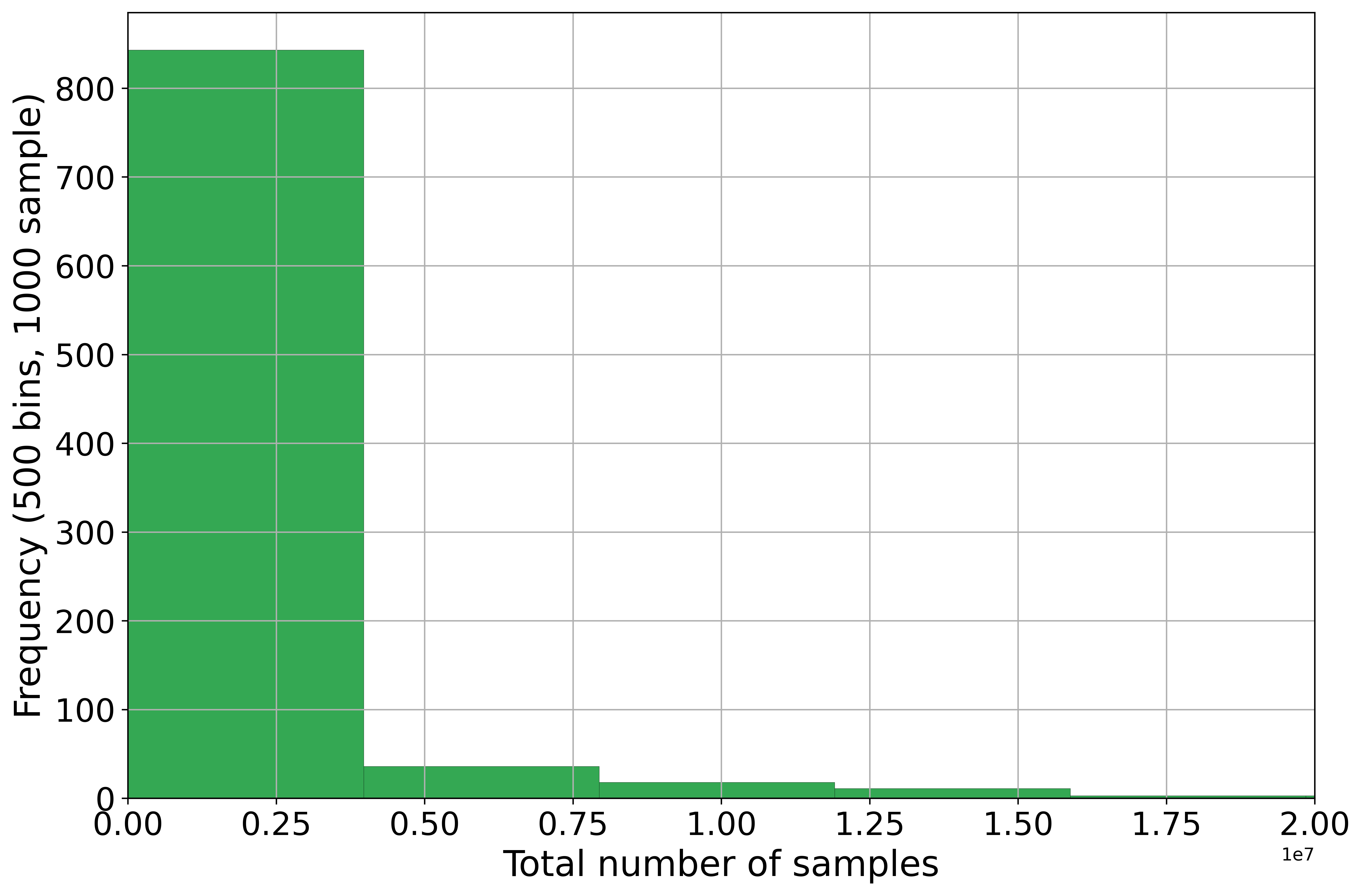
Figure 6: The histogram of the total number of samples for different $\theta$ of EJM measurement.

To gain deeper insights into the hardness of the estimation process, we graphically represented the average sample complexity and the bounding results in terms of stabilizer Rényi entropy, as depicted in Fig. 7. This visualization encompasses diverse parameter values of $\theta$ from Eq. (33) in the context of EJM. Notably, the average sample complexity is consistently bounded by stabilizer Rényi entropies of the target state across all chosen EJM parameters. The results presented in Fig. 7 also unveil that the sample complexities exhibit small variation with respect to the EJM parameters. Moreover, Protocol 1 achieves a consistently reduced average sample complexity when juxtaposed with Protocol 3. However, the stabilizer Rényi entropy bounds of the direct Protocol 3 are much tighter than those of Protocol 1, indicating that Protocol 1 might have a larger fluctuation in sample complexity.

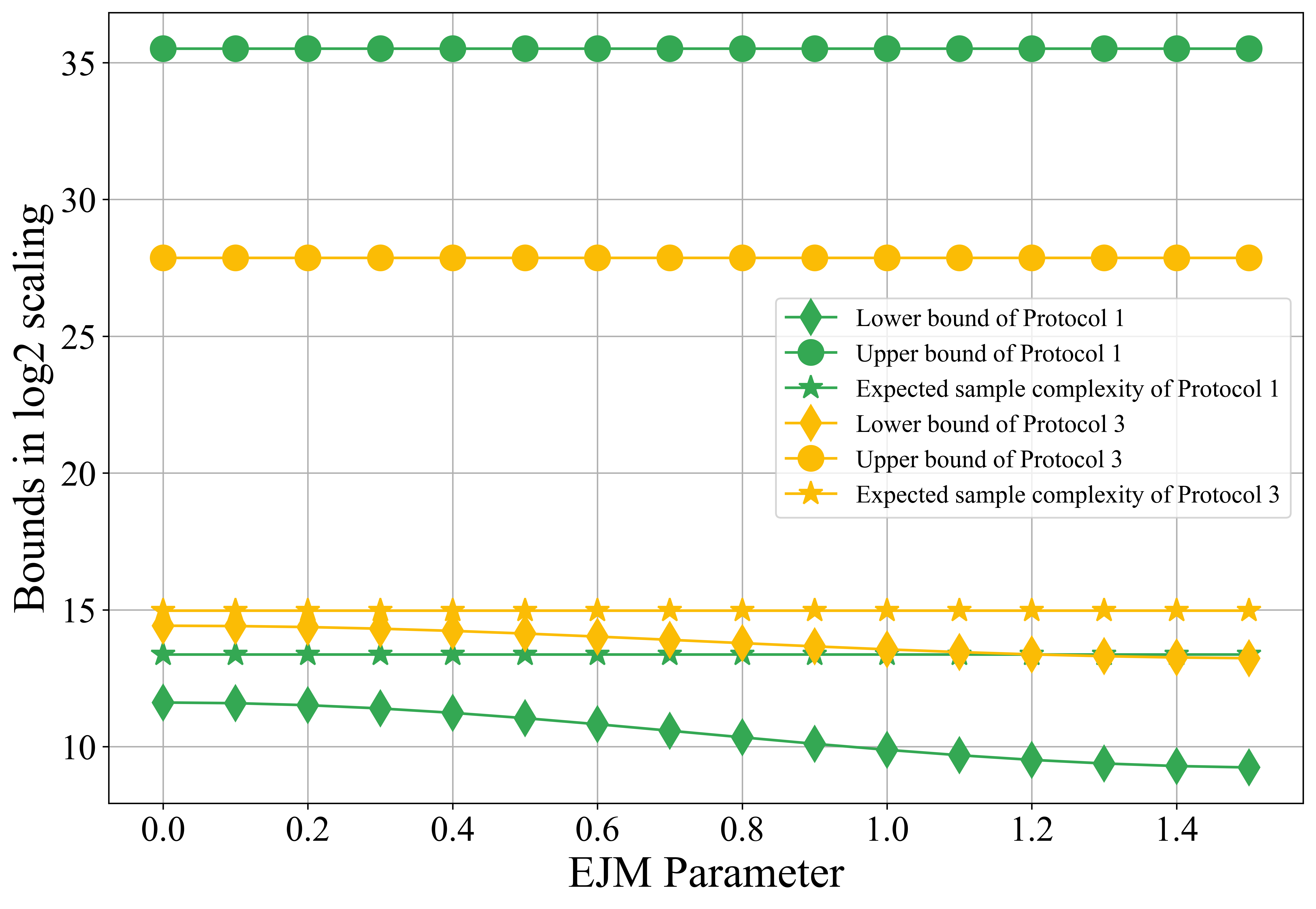
Figure 7: Comparisons of the expected sample complexity and the stabilizer Rényi entropy bounds of Protocol 1 and Protocol 3.

5 Conclusions

We have introduced an efficient protocol for estimating the performance of quantum measurements, leveraging the preparation and measurement of product eigenstates of Pauli operators. This protocol confers several advantages over existing methods, surpassing the speed of detector tomography and demonstrating an exponential acceleration compared to the direct fidelity estimation protocol for measurement devices. Furthermore, in specific scenarios, such as well-conditioned quantum measurements, our protocol demands only a constant number of measurement calls. This protocol is not only applicable to symmetric informationally complete POVMs and quantum measurements relying on mutually unbiased bases [RBKSC04, AS10, CGGŻ20], but also the most general positive operator-valued measure measurements via Naimark’s theorem. Its significance lies in its ability to facilitate the development of reliable quantum devices and propel continuous enhancements in their performances. Our protocol opens up new possibilities for certifying quantum measurements to high accuracy, providing a valuable tool for advancing the field of quantum information processing and enabling the realization of reliable and high performance quantum measurement devices.

The quest for even more efficient fidelity estimation lies in navigating the intricacies of sophisticated sampling strategies and adaptive approaches. This path presents exciting challenges and opportunities to minimize variance and sample complexity, ultimately yielding sharper accuracy and broader applicability of quantum measurements.

Acknowledgements.—This work was done when Z. S. was a research intern at Baidu Research.

Appendix A Proof of Theorem 1

Before delving into the sample complexity analysis summarized in Theorem 1 (see also Algorithm 1), we first present some essential lemmas.

Lemma 7.

Let $A$ and $B$ be two positive semidefinite operators, we have $\operatorname{Tr}[AB]\geq 0$.

Proof.

By the spectral theorem, we have

$$\operatorname{Tr}[AB] =\operatorname{Tr}\left[\sum_{i}\alpha_{i}|\phi_{i}\rangle\langle\phi_{i}|\sum_{j}\beta_{j}|\psi_{j}\rangle\langle\psi_{j}|\right]$$ (34)

$$=\sum_{ij}\alpha_{i}\beta_{j}\langle\phi_{i}|\psi_{j}\rangle\langle\psi_{j}|\phi_{i}\rangle$$ (35)

$$=\sum_{ij}\alpha_{i}\beta_{j}|\langle\phi_{i}|\psi_{j}\rangle|^{2}$$ (36)

Since $$A,B \alpha_{i}\geq 0 \beta_{j}\geq 0$$ are positive semidefinite, and

$$\geq 0.$$ (37)

∎

Lemma 8.

Let $\left\{V_{k}\right\}_{k}$ be a set of POVM elements satisfying $\sum_{k=1}^{2^{n}}V_{k}=\operatorname{id}$, where $n$ is the number of qubits. We then have

$$\sum_{k=1}^{2^{n}}\operatorname{Tr}[V_{k}^{2}] \leq 2^{n}.$$ (38)

Proof.

$$\operatorname{Tr}\left[\sum_{k=1}^{2^{n}}V_{k}^{2}\right] =\operatorname{Tr}\left[\sum_{k=1}^{2^{n}}V_{k}\sum_{j=1}^{2^{n}}V_{j}\right]-\operatorname{Tr}\left[\sum_{k\neq j}V_{k}V_{j}\right]$$ (39)

$$=\operatorname{Tr}[\operatorname{id}]-\operatorname{Tr}\left[\sum_{k\neq j}V_{k}V_{j}\right]$$ (40)

By lemma (7), we have $$\sum_{k\neq j}\operatorname{Tr}[V_{k}V_{j}]\geq 0$$

$$\leq 2^{n}.$$ (41)

∎

Proof of Theorem 1.

To commence, we begin with bounding the estimation error from the sample mean in step (11) of the efficient Protocol 1. Recognizing that $X_{l}$ is an unbounded random variable, we employ Chebyshev’s inequality to derive a tail bound for the estimation $Y$ in Eq. (7). Employing the definitions of the $q_{l}$ and $X_{l}$, we analyze the variance of $X_{l}$ as

$${\rm Var}[X_{l}] =\sum_{l=1}^{4^{n}}\left(\sum_{k^{\prime}=1}^{2^{n}}\frac{\operatorname{Tr}[\psi_{k\textquoteright}P_{l}]^{2}}{2^{n}}\right)\times\left(\sum_{k=1}^{2^{n}}\operatorname{Tr}[V_{k}P_{l}]\frac{\operatorname{Tr}[\psi_{k}P_{l}]}{\sum_{k^{\prime}=1}^{2^{n}}\operatorname{Tr}[\psi_{k\textquoteright}P_{l}]^{2}}\right)^{2}-F^{2}$$ (42)

$$\leq\sum_{l=1}^{4^{n}}\frac{\sum_{k^{\prime}=1}^{2^{n}}\operatorname{Tr}[\psi_{k\textquoteright}P_{l}]^{2}}{2^{n}}\times\frac{\left[\sum_{k=1}^{2^{n}}\operatorname{Tr}[V_{k}P_{l}]\operatorname{Tr}[\psi_{k}P_{l}]\right]^{2}}{\left[\sum_{k^{\prime}=1}^{2^{n}}\operatorname{Tr}[\psi_{k\textquoteright}P_{l}]^{2}\right]^{2}}$$ (43)

$$=\sum_{l=1}^{4^{n}}\frac{\left[\sum_{k=1}^{2^{n}}\operatorname{Tr}[V_{k}P_{l}]\operatorname{Tr}[\psi_{k}P_{l}]\right]^{2}}{2^{n}\left(\sum_{k^{\prime}=1}^{2^{n}}\operatorname{Tr}[\psi_{k\textquoteright}P_{l}]^{2}\right)}$$ (44)

Cauchy–Schwarz inequality

$$\leq\sum_{l=1}^{4^{n}}\frac{\left(\sum_{k=1}^{2^{n}}\operatorname{Tr}[V_{k}P_{l}]^{2}\right)\left(\sum_{k=1}^{2^{n}}\operatorname{Tr}[\psi_{k}P_{l}]^{2}\right)}{2^{n}\left(\sum_{k^{\prime}=1}^{2^{n}}\operatorname{Tr}[\psi_{k\textquoteright}P_{l}]^{2}\right)}$$ (45)

$$=\frac{\sum_{l=1}^{4^{n}}\sum_{k=1}^{2^{n}}\operatorname{Tr}[V_{k}P_{l}]^{2}}{2^{n}}$$ (46)

$$=\frac{\sum_{k=1}^{2^{n}}\operatorname{Tr}[V_{k}^{2}]}{2^{n}}$$ (47)

By lemma (8) (48)

$$\leq 1.$$ (49)

Hence, it is adequate to sample $m=\lceil 1/(\varepsilon^{2}\delta)\rceil$ number of Pauli operators, and the estimation of $\mathcal{F}$ can be expressed as

$$Y=\frac{1}{m}\sum_{i=1}^{m}X_{l_{i}}.$$ (50)

This formulation results in the $\varepsilon$-close estimator in Eq. (8) as guaranteed by Chebyshev’s inequality.

Next, we bound the estimation error of $X_{l_{i}}$ in step (9) of the efficient Protocol 1. We show that $\widehat{X}_{a_{j}}^{(l_{i})}$ is an unbiased estimator for a fixed $l_{i}$, since

$$\mathbb{E}[\widehat{X}_{a_{j}}^{(l_{i})}] =\mathbb{E}\left[\frac{2^{n}}{\sum_{k^{\prime}=1}^{2^{n}}\operatorname{Tr}[\psi_{k\textquoteright}P_{l_{i}}]^{2}}\times\lambda^{(l_{i})}_{a_{j}}\times\delta_{ko_{j}}\operatorname{Tr}[\psi_{o_{j}}P_{l_{i}}]\right]$$ (51)

$$=\mathbb{E}\left[\frac{2^{n}}{\sum_{k^{\prime}=1}^{2^{n}}\operatorname{Tr}[\psi_{k\textquoteright}P_{l_{i}}]^{2}}\times\lambda^{(l_{i})}_{a_{j}}\times\sum_{k=1}^{2^{n}}\delta_{ko_{j}}\operatorname{Tr}[\psi_{k}P_{l_{i}}]\right]$$ (52)

$$=\mathbb{E}_{a_{j}}\left[\frac{2^{n}}{\sum_{k^{\prime}=1}^{2^{n}}\operatorname{Tr}[\psi_{k\textquoteright}P_{l_{i}}]^{2}}\times\lambda^{(l_{i})}_{a_{j}}\times\sum_{k=1}^{2^{n}}\mathbb{E}[\delta_{ko_{j}}]\operatorname{Tr}[\psi_{k}P_{l_{i}}]\right]$$ (53)

$$=\mathbb{E}_{a_{j}}\left[\frac{2^{n}}{\sum_{k^{\prime}=1}^{2^{n}}\operatorname{Tr}[\psi_{k\textquoteright}P_{l_{i}}]^{2}}\times\lambda^{(l_{i})}_{a_{j}}\times\sum_{k=1}^{2^{n}}\operatorname{Tr}[V_{k}\phi_{a_{j}}^{(l_{i})}]\operatorname{Tr}[\psi_{k}P_{l_{i}}]\right]$$ (54)

$$=\sum_{a_{j}=1}^{2^{n}}\frac{1}{2^{n}}\times\frac{2^{n}}{\sum_{k^{\prime}=1}^{2^{n}}\operatorname{Tr}[\psi_{k\textquoteright}P_{l_{i}}]^{2}}\times\lambda^{(l_{i})}_{a_{j}}\sum_{k=1}^{2^{n}}\operatorname{Tr}[V_{k}\phi_{a_{j}}^{(l_{i})}]\operatorname{Tr}[\psi_{k}P_{l_{i}}]$$ (55)

$$=\frac{1}{\sum_{k^{\prime}=1}^{2^{n}}\operatorname{Tr}[\psi_{k\textquoteright}P_{l_{i}}]^{2}}\sum_{k=1}^{2^{n}}\operatorname{Tr}\left[V_{k}P_{l_{i}}\right]\operatorname{Tr}[\psi_{k}P_{l_{i}}]$$ (56)

$$\equiv X_{l_{i}},$$ (57)

where $\delta_{ko_{j}}=1$ if $k=o_{j}$ and $\delta_{ko_{j}}=0$ otherwise. Run step (6) and step (7) in the efficient Protocol 1 a total number of $n_{l_{i}}$ times, the estimation of $X_{l_{i}}$ is

$$\widetilde{X}_{l_{i}} =\frac{1}{n_{l_{i}}}\sum_{j=1}^{n_{l_{i}}}\widehat{X}_{a_{j}}^{(l_{i})}=\frac{1}{n_{l_{i}}}\sum_{j=1}^{n_{l_{i}}}\frac{2^{n}}{\sum_{k^{\prime}=1}^{2^{n}}\operatorname{Tr}[\psi_{k\textquoteright}P_{l_{i}}]^{2}}\times\lambda^{(l_{i})}_{a_{j}}\times\delta_{ko_{j}}\times\operatorname{Tr}[\psi_{o_{j}}P_{l_{i}}].$$ (58)

Then, we consider the double sum

$$m\widetilde{Y}=\sum_{i=1}^{m}\widetilde{X}_{l_{i}}=\sum_{i=1}^{m}\sum_{j=1}^{n_{l_{i}}}\underbrace{\frac{1}{n_{l_{i}}}\frac{2^{n}}{\sum_{k^{\prime}=1}^{2^{n}}\operatorname{Tr}[\psi_{k\textquoteright}P_{l_{i}}]^{2}}\times\lambda^{(l_{i})}_{a_{j}}\times\delta_{ko_{j}}\times\operatorname{Tr}[\psi_{o_{j}}P_{l_{i}}]}_{C_{ij}}.$$ (59)

Since $\lambda^{(l_{i})}_{a_{j}}=\pm 1/\sqrt{2^{n}}$, $\delta_{ko_{j}}=0$ when $k\neq o_{j}$ and $1$ otherwise, and $|\operatorname{Tr}[\psi_{o_{j}}P_{l_{i}}]|\leq 1/\sqrt{2^{n}}$, for a fixed $l_{i}$, the upper bound $b_{l_{i}}$ and the lower bound $a_{l_{i}}$ of $C_{ij}$ is

$$b_{l_{i}}=-a_{l_{i}}=\frac{1}{n_{l_{i}}}\frac{1}{\sum_{k^{\prime}=1}^{2^{n}}\operatorname{Tr}[\psi_{k\textquoteright}P_{l_{i}}]^{2}}.$$ (60)

We use the Hoeffding’s inequality to bound the estimation error as:

$${\rm Pr}(|\widetilde{Y}-Y|\geq\varepsilon)={\rm Pr}(|m\widetilde{Y}-mY|\geq\varepsilon)\leq 2\exp(-2m^{2}\varepsilon^{2}/C),$$ (61)

where $C=\sum_{i=1}^{m}\sum_{j=1}^{n_{l_{i}}}(2/(n_{l_{i}}\sum_{k^{\prime}=1}^{2^{n}}\operatorname{Tr}[\psi_{k^{\prime}}P_{l_{i}}]^{2}))^{2}$. Now choose

$$n_{l_{i}}=\left\lceil\frac{2}{m\left(\sum_{k^{\prime}=1}^{2^{n}}\operatorname{Tr}[\psi_{k\textquoteright}P_{l_{i}}]^{2}\right)^{2}\varepsilon^{2}}\ln\frac{2}{\delta}\right\rceil=\left\lceil\frac{1}{(\sum_{k^{\prime}=1}^{2^{n}}\operatorname{Tr}[\psi_{k\textquoteright}P_{l_{i}}]^{2})^{2}}\times\frac{2}{m\varepsilon^{2}}\ln\frac{2}{\delta}\right\rceil.$$ (62)

We have

$$\frac{1}{m^{2}}C =\sum_{i=1}^{m}\sum_{j=1}^{n_{l_{i}}}4\frac{1}{m^{2}n_{l_{i}}^{2}}\frac{1}{(\sum_{k^{\prime}=1}^{2^{n}}\operatorname{Tr}[\psi_{k\textquoteright}P_{l_{i}}]^{2})^{2}}$$ (63)

$$=\sum_{l=1}^{m}4\frac{1}{m^{2}n_{l_{i}}}\frac{1}{(\sum_{k^{\prime}=1}^{2^{n}}\operatorname{Tr}[\psi_{k\textquoteright}P_{l_{i}}]^{2})^{2}}$$ (64)

$$\leq\sum_{i=1}^{m}\frac{1}{m}\frac{2\varepsilon^{2}}{\ln(2/\delta)}$$ (65)

$$=\frac{2\varepsilon^{2}}{\ln(2/\delta)},$$ (66)

which guarantees the confidence interval (14). By combination of Eqs. (8) and (14), we arrive at the final estimator $\widetilde{Y}$ satisfying the confidence interval (16).

To determine the expected number of times the measurement device needs to be accessed, it is crucial to acknowledge that $n_{l}$ is a random variable, as $l$ is selected randomly. By the definition of sampling, for a fixed $l$, we have

$$\mathbb{E}[n_{l}] =\sum_{l=1}^{|\mathcal{S}|}q_{l}n_{l}$$ (67)

$$\geq\sum_{l=1}^{|\mathcal{S}|}\frac{\sum_{k^{\prime}=1}^{2^{n}}\operatorname{Tr}[\psi_{k\textquoteright}P_{l}]^{2}}{2^{n}}\times\left(\frac{2}{m\left(\sum_{k^{\prime}=1}^{2^{n}}\operatorname{Tr}[\psi_{k\textquoteright}P_{l}]^{2}\right)^{2}\varepsilon^{2}}\log\frac{2}{\delta}\right)$$ (68)

$$=\left(\sum_{l=1}^{|\mathcal{S}|}\frac{1}{2^{n}\sum_{k^{\prime}=1}^{2^{n}}\operatorname{Tr}[\psi_{k\textquoteright}P_{l}]^{2}}\right)\times\frac{2}{m\varepsilon^{2}}\log\frac{2}{\delta}.$$ (69)

Due to the HM-GM-AM-QM inequalities, we have

$${\left(\sum_{l=1}^{|\mathcal{S}|}\frac{1}{2^{n}\sum_{k^{\prime}=1}^{2^{n}}\operatorname{Tr}[\psi_{k\textquoteright}P_{l}]^{2}}\right)}\geq\frac{|\mathcal{S}|^{2}}{2^{n}\sum_{l=1}^{|\mathcal{S}|}{\sum_{k^{\prime}=1}^{2^{n}}\operatorname{Tr}[\psi_{k\textquoteright}P_{l}]^{2}}}=\frac{|\mathcal{S}|^{2}}{4^{n}}.$$ (70)

Thus, we get

$$\mathbb{E}[L]=\sum_{i=1}^{m}\mathbb{E}[n_{l_{i}}]\geq{\frac{|\mathcal{S}|^{2}}{4^{n}}}\frac{2}{\varepsilon^{2}}\ln\frac{2}{\delta}.$$ (71)

It is noteworthy that the maximum cardinality of $|\mathcal{S}|$ is $4^{n}$, signifying that the worst-case lower bound scales as $\Omega(4^{n})$. ∎

Appendix B Proof of Theorem 2

Proof of Theorem 2.

Recall the estimator (13) employed in the efficient protocol. Setting $n_{l_{i}}=1$, we obtain

$$\widetilde{Y} =\frac{1}{L}\sum_{i=1}^{L}\frac{2^{n}}{\sum_{k^{\prime}=1}^{2^{n}}\operatorname{Tr}[\psi_{k\textquoteright}P_{l_{i}}]^{2}}\times\lambda^{(l_{i})}_{a_{j}}\times\delta_{ko_{j}}\times\operatorname{Tr}[\psi_{o_{j}}P_{l_{i}}]\equiv\frac{1}{L}\sum_{i=1}^{L}C_{l_{i}}.$$ (72)

The upper bound $b_{l_{i}}$ and the lower bound $a_{l_{i}}$ of $C_{l_{i}}$ satisfy $b_{l_{i}}=-a_{l_{i}}=1/\sum_{k^{\prime}=1}^{2^{n}}\operatorname{Tr}[\psi_{k^{\prime}}P_{l_{i}}]^{2}$. Then, applying Hoeffding’s inequality, we obtain

$${\rm Pr}\left(\left|\widetilde{Y}-\mathcal{F}\right|\geq\varepsilon\right) ={\rm Pr}\left(\left|\sum_{i=1}^{L}C_{l_{i}}-L\mathcal{F}\right|\geq L\varepsilon\right)$$ (73)

$$\leq 2\exp\left[-\frac{L^{2}\varepsilon^{2}}{\sum_{i=1}^{L}\frac{2}{\left[\sum_{k=1}^{2^{n}}\operatorname{Tr}[\psi_{k}P_{l_{i}}]^{2}\right]^{2}}}\right]$$ (74)

$$\leq 2\exp\left[-\frac{L^{2}\varepsilon^{2}}{\sum_{i=1}^{L}\frac{2}{\mathbb{M}^{2}}}\right]$$ (75)

$$\leq\delta,$$ (76)

where

$$\mathbb{M} \mathrel{\mathop{\mathchar 58\relax}}=\min_{l}\sum_{k=1}^{2^{n}}\operatorname{Tr}[\psi_{k}P_{l}]^{2}=\min_{l}\operatorname{Tr}[OP_{l}]^{2}\cdot 2^{n}\leq\sqrt{\frac{\exp[-M_{2}(\mathcal{M})]}{2^{n}}}^{2}\cdot 2^{n}={\exp\left[-M_{2}(\mathcal{M})\right]}$$ (77)

by the definition of $O$ in Eq. (20) and $M_{\alpha}(\mathcal{M})$ in Eq. (21). Thus, we get the lower bound as

$$L\geq\frac{1}{\mathbb{M}^{2}}\cdot\frac{2}{\varepsilon^{2}}\ln\frac{2}{\delta}\geq\frac{2}{\varepsilon^{2}}\ln\frac{2}{\delta}\exp\left[2M_{2}(\mathcal{M})\right].$$ (78)

Now, let’s analyze the upper bound. Initially, we truncate the PVM elements $\psi_{k}$ as defined in Eq. (155), resulting in $\psi_{k}^{\prime}$. Subsequently, we employ these truncated PVM elements $\psi_{k}^{\prime}$ to approximate $\mathcal{F}$. The absolute difference is bounded as $|\mathcal{F}^{\prime}-\mathcal{F}|<{\varepsilon}/{2}$. The estimation $\widetilde{Y}^{\prime}$ of $\mathcal{F}^{\prime}$ is given by

$$\widetilde{Y}^{\prime} =\frac{1}{L}\sum_{i=1}^{L}\frac{2^{n}}{\sum_{k^{\prime}=1}^{2^{n}}\operatorname{Tr}[\psi_{k^{\prime}}^{\prime}P_{l_{i}}]^{2}}\times\lambda^{(l_{i})}_{a_{i}}\times\delta_{ko_{i}}\times\operatorname{Tr}[\psi_{o_{i}}P_{l_{i}}]\equiv\frac{1}{L}\sum_{i=1}^{L}C_{l_{i}}^{\prime}.$$ (79)

The upper bound $b_{l_{i}}^{\prime}$ and the lower bound $a_{l_{i}}^{\prime}$ of $C_{l_{i}}^{\prime}$ satisfy $b_{l_{i}}^{\prime}=-a_{l_{i}}^{\prime}=1/\sum_{k^{\prime}=1}^{2^{n}}\operatorname{Tr}[\psi_{k^{\prime}}^{\prime}P_{l_{i}}]^{2}$. It can be demonstrated that $\mathbb{E}[C_{l_{i}}^{\prime}]=\mathcal{F}$. Subsequently, by applying Hoeffding’s inequality, we obtain

$${\rm Pr}\left(|\widetilde{Y}^{\prime}-\mathcal{F}^{\prime}|\leq\frac{\varepsilon}{2}\right) ={\rm Pr}\left(\left|\sum_{i=1}^{L}C_{l_{i}}^{\prime}-L\mathcal{F}^{\prime}\right|\geq\frac{L\varepsilon}{2}\right)$$ (80)

$$\geq 1-2\exp\left[-\frac{L^{2}\varepsilon^{2}/4}{\sum_{i=1}^{L}(b_{l_{i}}^{\prime}-a_{l_{i}}^{\prime})^{2}}\right]$$ (81)

$$\geq 1-2\exp\left[-\frac{L^{2}\varepsilon^{2}}{\sum_{i=1}^{L}\frac{16}{\mathbb{M}^{\prime 2}}}\right]$$ (82)

$$=1-\delta,$$ (83)

where $\mathbb{M}^{\prime}\mathrel{\mathop{\mathchar 58\relax}}=\min_{l}\sum_{k=1}^{2^{n}}\operatorname{Tr}[\psi_{k}^{\prime}P_{l}]^{2}$. This leads to

$$L=\frac{16}{\mathbb{M}^{\prime 2}}\cdot\frac{1}{\varepsilon^{2}}\ln\frac{2}{\delta}.$$ (84)

Now, we derive:

$$\mathbb{M}^{\prime}=\min_{l}\sum_{k=1}^{2^{n}}\operatorname{Tr}[\psi_{k}^{\prime}P_{l}]^{2} \geq\min_{l}\sum_{k=1}^{2^{n}}\operatorname{Tr}[\psi_{k,cut}P_{l}]^{2}$$ (85)

$$\geq\min_{l}\sum_{k=1}^{2^{n}}\left[\frac{\varepsilon}{2\sqrt{2}}\sqrt{\frac{\exp[-M_{0}(\psi_{k})]}{2^{n}}}\right]^{2}$$ (86)

$$=\sum_{k=1}^{2^{n}}\frac{\varepsilon^{2}}{8}\frac{\exp[-M_{0}(\psi_{k})]}{2^{n}}$$ (87)

$$\geq\sum_{k=1}^{2^{n}}\frac{\varepsilon^{2}}{8}\frac{\exp[-M_{0}(\mathcal{M})]}{2^{n}}$$ (88)

$$=\frac{\varepsilon^{2}}{8}{\exp[-M_{0}(\mathcal{M})]},$$ (89)

Finally, the upper bound is obtained as

$$L=\frac{16}{\mathbb{M}^{\prime 2}}\cdot\frac{1}{\varepsilon^{2}}\ln\frac{2}{\delta}\leq\frac{2^{10}}{\varepsilon^{6}}\ln\frac{2}{\delta}\exp[2M_{0}(\mathcal{M})],$$ (90)

Substituting $\varepsilon$ and $\delta$ with $2\varepsilon$ and $2\delta$, respectively, yields Theorem 2, presenting the bounding results for a $2\varepsilon$-close estimator. ∎

Appendix C Proof of Theorem 3

Proof of Theorem 3.

It follows directly from Eq. (24) that $\mathbb{E}[\widetilde{X}_{k_{i}}]=\mathcal{F}$. We also note that $\widetilde{X}_{k_{i}}\in\{0,1\}$. Thus, by Hoeffding’s inequality, we get

$${\rm Pr}\left(|\widetilde{Y}-\mathcal{F}|\geq\varepsilon\right) ={\rm Pr}\left(\left|\sum_{i=1}^{L}\widetilde{X}_{k_{i}}-L\mathcal{F}\right|\geq L\varepsilon\right)$$ (91)

$$\leq 2\exp\left[-\frac{2L^{2}\varepsilon^{2}}{\sum_{i=1}^{L}(1-0)^{2}}\right]$$ (92)

$$=2\exp\left[-2L\varepsilon^{2}\right]$$ (93)

$$\leq\delta,$$ (94)

which implies that

$$L\geq\frac{1}{2\varepsilon^{2}}\ln\frac{2}{\delta}.$$ (95)

This leads to a $\varepsilon$-close estimator

$${\rm Pr}\left(|\widetilde{Y}-\mathcal{F}|\geq\varepsilon\right)\leq\delta.$$ (96)

By substituting $\varepsilon$ and $\delta$ with $2\varepsilon$ and $2\delta$, respectively, we conclude Theorem 3. ∎

Appendix D Details of the direct protocol

Now we proceed to formulate the direct protocol. First, we rewrite the measurement fidelity $\mathcal{F}$ as

$$\mathcal{F} =\frac{1}{2^{n}}\sum_{k=1}^{2^{n}}\operatorname{Tr}[\psi_{k}V_{k}]$$ (97)

$$=\frac{1}{2^{n}}\sum_{k=1}^{2^{n}}\sum_{l=1}^{4^{n}}\operatorname{Tr}[\psi_{k}P_{l}]\operatorname{Tr}[V_{k}P_{l}]$$ (98)

$$=\sum_{k=1}^{2^{n}}\sum_{l=1}^{4^{n}}\frac{\operatorname{Tr}[\psi_{k}P_{l}]^{2}}{2^{n}}\frac{\operatorname{Tr}[V_{k}P_{l}]}{\operatorname{Tr}[\psi_{k}P_{l}]}$$ (99)

$$\equiv\sum_{k=1}^{2^{n}}\sum_{l=1}^{4^{n}}q_{kl}X_{kl},$$ (100)

where $q_{kl}\mathrel{\mathop{\mathchar 58\relax}}={\operatorname{Tr}[\psi_{k}P_{l}]^{2}}/{2^{n}}$ forms a joint probability mass function and $X_{kl}\mathrel{\mathop{\mathchar 58\relax}}={\operatorname{Tr}[V_{k}P_{l}]}/{\operatorname{Tr}[\psi_{k}P_{l}]}$ denotes a random variable. It can be demonstrated that $\mathbb{E}[X_{kl}]=\mathcal{F}$, indicating that $X_{kl}$ serves as an unbiased estimator for $\mathcal{F}$. Consequently, we can formulate an estimator for $\mathcal{F}$ utilizing the sample mean. We perform joint sampling $k$ and $l$ multiple times according to the probability distribution $q_{kl}$, resulting in $m$ pairs $(k_{1},l_{1}),(k_{2},l_{2}),...,(k_{m},l_{m})$. We choose $m$ as

$$m=\left\lceil 1/(\varepsilon^{2}\delta)\right\rceil.$$ (101)

Then, we estimate $\mathcal{F}$ using the following formula:

$$Y=\frac{1}{m}\sum_{i=1}^{m}X_{k_{i}l_{i}}.$$ (102)

This leads to a $\varepsilon$-accurate estimator as

$${\rm Pr}\left(|Y-\mathcal{F}|\geq\varepsilon\right)\leq\delta.$$ (103)

Subsequently, we proceed to estimate $X_{k_{i}l_{i}}$ using the measurement outcomes. Given that $P_{l}$ is not a quantum state, we must execute the spectral decomposition

$$P_{l}=\sum_{a=1}^{2^{n}}\lambda_{a}^{(l)}{|\phi_{a}^{(l)}\rangle\langle\phi_{a}^{(l)}|}\equiv\sum_{a=1}^{2^{n}}\lambda_{a}^{(l)}\phi_{a}^{(l)}.$$ (104)

Rewrite $X_{k_{i}l_{i}}$ as

$$X_{k_{i}l_{i}} =\sum_{a=1}^{2^{n}}\lambda_{a}^{(l_{i})}\frac{\operatorname{Tr}[V_{k_{i}}\phi_{a}^{(l_{i})}]}{\operatorname{Tr}[\psi_{k_{i}}P_{l_{i}}]}.$$ (105)

Next, $\operatorname{Tr}[V_{k_{i}}\phi_{a}^{(l_{i})}]$ can be estimated by performing measurements on $\phi_{a}^{(l_{i})}$ multiple times. The subroutine for this process is outlined below:

• Sample an index. Choose a random index $a_{j}$, where $a_{j}\in\{1,2,\cdots,2^{n}\}$ uniformly;

• Measure the eigenstate. Utilize the quantum measurement device to measure the eigenstate $\phi^{(l_{i})}_{a_{j}}$ (associated with $P_{l_{i}}$) and record the experimental outcome $o_{j}$.

Define a new random variable $\widehat{X}_{k_{i}l_{i}}$ as

$$\widehat{X}_{k_{i}l_{i}}=\frac{2^{n}}{\operatorname{Tr}[\psi_{k_{i}}P_{l_{i}}]}\times\lambda_{a_{j}}^{(l_{i})}\times\delta_{k_{i}o_{j}},$$ (106)

and it can be demonstrated that $\mathbb{E}[\widehat{X}_{k_{i}l_{i}}]$ is an unbiased estimator as follows:

$$\mathbb{E}[\widehat{X}_{k_{i}l_{i}}] =\mathbb{E}\left[\frac{2^{n}}{\operatorname{Tr}[\psi_{k_{i}}P_{l_{i}}]}\times\lambda_{a_{j}}^{(l_{i})}\times\delta_{k_{i}o_{j}}\right]$$ (107)

$$=\mathbb{E}_{a_{j}}\left[\frac{2^{n}}{\operatorname{Tr}[\psi_{k_{i}}P_{l_{i}}]}\times\lambda_{a_{j}}^{(l_{i})}\times\mathbb{E}[\delta_{k_{i}o_{j}}]\right]$$ (108)

$$=\mathbb{E}_{a_{j}}\left[\frac{2^{n}}{\operatorname{Tr}[\psi_{k_{i}}P_{l_{i}}]}\times\lambda_{a_{j}}^{(l_{i})}\times\operatorname{Tr}[V_{k_{i}}\phi_{a_{j}}^{(l_{i})}]\right]$$ (109)

$$=\sum_{a_{j}=1}^{2^{n}}\frac{1}{2^{n}}\times\frac{2^{n}}{\operatorname{Tr}[\psi_{k_{i}}P_{l_{i}}]}\lambda_{a_{j}}^{(l_{i})}\operatorname{Tr}[V_{k_{i}}\phi_{a_{j}}^{(l_{i})}]$$ (110)

$$=\frac{\operatorname{Tr}[V_{k_{i}}P_{l_{i}}]}{\operatorname{Tr}[\psi_{k_{i}}P_{l_{i}}]}\equiv X_{k_{i}l_{i}}$$ (111)

By running this procedure a total number of $n_{l_{i}}$ times, we can estimate $X_{k_{i}l_{i}}$ as

$$\widetilde{X}_{k_{i}l_{i}}=\frac{1}{n_{l_{i}}}\sum_{j=1}^{n_{l_{i}}}\widehat{X}_{k_{i}l_{i}}=\frac{1}{n_{i}}\sum_{j=1}^{n_{i}}\frac{2^{n}}{\operatorname{Tr}[\psi_{k_{i}}P_{l_{i}}]}\times\lambda_{a_{j}}^{(l_{i})}\times\delta_{k_{i}o_{j}},$$ (112)

where Our estimator of $Y$ is

$$\widetilde{Y} =\frac{1}{m}\sum_{i=1}^{m}\widetilde{X}_{k_{i}l_{i}}$$ (113)

$$=\sum_{i=1}^{m}\sum_{j=1}^{n_{l_{i}}}\frac{1}{mn_{l_{i}}}\frac{2^{n}}{\operatorname{Tr}[\psi_{k_{i}}P_{l_{i}}]}\times\lambda_{a_{j}}^{(l_{i})}\times\delta_{k_{i}o_{j}},$$ (114)

where $\delta_{k_{i}o_{j}}=1$ if $k_{i}=o_{j}$ and $\delta_{k_{i}o_{j}}=0$ otherwise. To satisfy the confidence interval

$${\rm Pr}\left(|\widetilde{Y}-Y|\geq\varepsilon\right)\leq\delta,$$ (115)

we choose

$$n_{l_{i}} =\left\lceil\frac{1}{\operatorname{Tr}[\psi_{k_{i}}P_{l_{i}}]^{2}}\frac{2\cdot 2^{n}}{m\varepsilon^{2}}\ln{\frac{2}{\delta}}\right\rceil,$$ (116)

By combining the confidence intervals (103) and (115) using the union bound, we deduce the confidence interval for the final estimation $\widetilde{Y}$ as

$${\rm Pr}\left\{|\widetilde{Y}-\mathcal{F}|\geq 2\varepsilon\right\}\leq 2\delta.$$ (117)

Appendix E Proof of Theorem 4

Proof of Theorem 4.

First, we bound the estimation error from the sample mean in step (11) of the direct Protocol 3. We note that $X_{kl}$ is an unbounded random variable; thus we employ Chebyshev’s inequality [KR21] to derive a tail bound for the estimation $Y$ in Eq. (102). Using the definitions of the $q_{kl}$ and $X_{kl}$, we investigate the variance of $X_{kl}$ and obtain

$${\rm Var}(X_{kl}) =\mathbb{E}\left[X_{kl}^{2}\right]-\mathbb{E}\left[X_{kl}\right]^{2}$$ (118)

$$=\sum_{k=1}^{2^{n}}\sum_{l=1}^{4^{n}}\frac{\operatorname{Tr}[\psi_{k}P_{l}]^{2}}{2^{n}}\times\frac{\operatorname{Tr}[V_{k}P_{l}]^{2}}{\operatorname{Tr}[\psi_{k}P_{l}]^{2}}-\left[\sum_{k=1}^{2^{n}}\sum_{l=1}^{4^{n}}\frac{\operatorname{Tr}[\psi_{k}P_{l}]^{2}}{2^{n}}\times\frac{\operatorname{Tr}[V_{k}P_{l}]}{\operatorname{Tr}[\psi_{k}P_{l}]}\right]^{2}$$ (119)

$$=\sum_{k=1}^{2^{n}}\sum_{l=1}^{4^{n}}\frac{\operatorname{Tr}[V_{k}P_{l}]^{2}}{2^{n}}-\mathcal{F}^{2}$$ (120)

$$\leq\sum_{k=1}^{2^{n}}\frac{\sum_{l=1}^{4^{n}}\operatorname{Tr}[V_{k}P_{l}]^{2}}{2^{n}}$$ (121)

$$=\sum_{k=1}^{2^{n}}\frac{\operatorname{Tr}[V_{k}^{2}]}{2^{n}}$$ (122)

By lemma (8)

$$\leq 1.$$ (123)

Therefore, we can bound the the variance of $Y$ as

$${\rm Var}(Y) =\frac{1}{m^{2}}\sum_{i=1}^{m}{\rm Var}(X_{k_{i}l_{i}})\in\left[0,\frac{1}{m}\right].$$ (124)

Then, by Chebyshev’s inequality, we have

$${\rm Pr}\left(|Y-\mathcal{F}|\geq\varepsilon\right)\leq\frac{{\rm Var}(Y)}{\varepsilon^{2}}\leq\frac{1}{\varepsilon^{2}m}.$$ (125)

Let $m={1}/{\lceil\varepsilon^{2}\delta\rceil}$, we have Eq. (103). Now we bound the estimation error of $X_{k_{i}l_{i}}$ in step (9) of the direct Protocol 3. We have shown that $\widehat{X}_{k_{i}l_{i}}$ is an unbiased estimator; thus we we use the empirical mean (112) to estimate $X_{k_{i}l_{i}}$. Then we consider the double sum as

$$m\widetilde{Y} =\sum_{i=1}^{m}\widetilde{X}_{k_{i}l_{i}}=\sum_{i=1}^{m}\sum_{j=1}^{n_{l_{i}}}C_{k_{i}l_{i}o_{j}},$$ (126)

where

$$C_{k_{i}l_{i}o_{j}}=\frac{2^{n}}{n_{l_{i}}\operatorname{Tr}[\psi_{k_{i}}P_{l_{i}}]}\times\lambda_{a_{j}}^{(l_{i})}\times\delta_{k_{i}o_{j}}.$$ (127)

Note that for a fixed pair $(k_{i},l_{i})$, the upper bound $b_{k_{i}l_{i}}$ and lower bound $a_{k_{i}l_{i}}$ of $C_{k_{i}l_{i}o_{j}}$ is

$$b_{k_{i}l_{i}}=-a_{k_{i}l_{i}}=\frac{\sqrt{2^{n}}}{n_{l_{i}}\operatorname{Tr}[\psi_{k_{i}}P_{l_{i}}]}.$$ (128)

By Hoeffding’s inequality [KR21], we have

$${\rm Pr}(|\widetilde{Y}-Y|\geq\varepsilon) ={\rm Pr}\left(\left|\sum_{i=1}^{m}\sum_{j=1}^{n_{k_{i}l_{i}}}C_{k_{i}l_{i}o_{j}}-mY\right|\geq m\varepsilon\right)$$ (129)

$$\leq 2\exp\left[-\frac{2m^{2}\varepsilon^{2}}{\sum_{i=1}^{m}\sum_{j=1}^{n_{k_{i}l_{i}}}\left(\frac{2\cdot\sqrt{2^{n}}}{n_{k_{i}l_{i}}\operatorname{Tr}[\psi_{k_{i}}P_{l_{i}}]}\right)^{2}}\right]$$ (130)

$$\leq 2\exp\left[-\frac{m^{2}\varepsilon^{2}}{\sum_{i=1}^{m}\sum_{j=1}^{n_{k_{i}l_{i}}}\frac{2\cdot{2^{n}}}{n_{k_{i}l_{i}}^{2}\operatorname{Tr}[\psi_{k_{i}}P_{l_{i}}]^{2}}}\right]$$ (131)

$$\leq\delta,$$ (132)

where $n_{k_{i}l_{i}}$ is chosen as

$$n_{k_{i}l_{i}} =\left\lceil\frac{1}{\operatorname{Tr}[\psi_{k_{i}}P_{l_{i}}]^{2}}\frac{2\cdot 2^{n}}{m\varepsilon^{2}}\ln{\frac{2}{\delta}}\right\rceil$$ (133)

to guarantee Eq. (115).

By combining confidence intervals (103) and (115) using the union bound, we establish the confidence interval for the final estimation $\widetilde{Y}$ concluded in Eq. (117).

To derive the expected value of the number of calls to the measurement device, we note that $n_{kl}$ is a random variable, since $(k,l)$ is randomly chosen. By definition, we have

$$\mathbb{E}[n_{k_{l}}] =\sum_{i=1}^{|\mathcal{T}|}q_{k_{i}l_{i}}n_{k_{i}l_{i}}$$ (134)

$$\leq 1+\sum_{(k_{i},l_{i})=1}^{|\mathcal{T}|}\frac{\operatorname{Tr}[\psi_{k_{i}}P_{l_{i}}]^{2}}{2^{n}}\times\frac{1}{\operatorname{Tr}[\psi_{k_{i}}P_{l_{i}}]^{2}}\frac{2\cdot 2^{n}}{m\varepsilon^{2}}\ln\frac{2}{\delta}$$ (135)

$$=1+\sum_{(k_{i},l_{i})=1}^{|\mathcal{T}|}\frac{2}{m\varepsilon^{2}}\ln\frac{2}{\delta}$$ (136)

$$=1+\frac{2|\mathcal{T}|}{m\varepsilon^{2}}\ln\frac{2}{\delta},$$ (137)

where $\mathcal{T}$ is defined in Eq. (31). Therefore, the expected value of the total number of calls $L=\sum_{i=1}^{m}n_{k_{i}l_{i}}$ is

$$\mathbb{E}[L] =\sum_{i=1}^{m}\mathbb{E}[n_{k_{i}l_{i}}]$$ (138)

$$\leq\sum_{i=1}^{m}\left[1+\frac{2|\mathcal{T}|}{m\varepsilon^{2}}\ln\frac{2}{\delta}\right]$$ (139)

$$\leq 1+\frac{1}{\varepsilon^{2}\delta}+2|\mathcal{T}|\frac{1}{\varepsilon^{2}}\ln\frac{2}{\delta}.$$ (140)

∎

Appendix F Proof of Theorem 5

Proof of Theorem 5.

Recall the estimator (113) in the direct Protocol 3. Here, we set $n_{k_{i}l_{i}}=1$ and have

$$\widetilde{Y} =\frac{1}{L}\sum_{i=1}^{L}\frac{2^{n}}{\operatorname{Tr}[\psi_{k_{i}}P_{l_{i}}]}\times\lambda_{a_{i}}^{l_{i}}\times\delta_{k_{i}o_{i}}\equiv\frac{1}{m}\sum_{i=1}^{m}C_{k_{i}l_{i}o_{i}},$$ (141)

and the upper bound $b_{k_{i}l_{i}}$ and the lower bound $a_{k_{i}l_{i}}$ of $C_{k_{i}l_{i}o_{i}}$ is $b_{k_{i}l_{i}}=-a_{k_{i}l_{i}}=\sqrt{2^{n}}/\operatorname{Tr}[\psi_{k_{i}}P_{l_{i}}]$. Then by Hoeffding’s inequality, we have

$${\rm Pr}(|\widetilde{Y}-Y|\geq\varepsilon) ={\rm Pr}\left(\left|\sum_{i=1}^{L}\frac{2^{n}}{\operatorname{Tr}[\psi_{k_{i}}P_{l_{i}}]}\times\lambda_{a_{i}}^{(l_{i})}\times\delta_{k_{i}o_{i}}-LY\right|\geq L\varepsilon\right)$$ (142)

$$\leq 2\exp\left[-\frac{2L^{2}\varepsilon^{2}}{\sum_{i=1}^{L}(b_{k_{i}l_{i}}-a_{k_{i}l_{i}})^{2}}\right]$$ (143)

$$=2\exp\left[-\frac{2L^{2}\varepsilon^{2}}{\sum_{i=1}^{L}\frac{4\cdot 2^{n}}{\operatorname{Tr}[\psi_{k_{i}}P_{l_{i}}]^{2}}}\right]$$ (144)

$$\leq 2\exp\left[-\frac{2L^{2}\varepsilon^{2}}{\sum_{i=1}^{L}\frac{4\cdot 2^{n}}{\mathbb{M}^{2}}}\right]$$ (145)

$$=2\exp\left[-\frac{L\varepsilon^{2}}{2\cdot 2^{n}\cdot\mathbb{M}^{-2}}\right]$$ (146)

$$\leq\delta,$$ (147)

where $\mathbb{M}\mathrel{\mathop{\mathchar 58\relax}}=\min_{k,l}|\operatorname{Tr}[\psi_{k}P_{l}]|$. Thus, we have

$$L \geq\frac{2\cdot 2^{n}}{\mathbb{M}^{2}}\frac{1}{\varepsilon^{2}}\ln\frac{2}{\delta}.$$ (148)

Now, we investigate the relationship between $\mathbb{M}$ and 2-stabilizer Reńyi entropy. It is noteworthy that

$$\mathbb{M}=\min_{k}\min_{l}|\operatorname{Tr}[\psi_{k}P_{l}] \leq\min_{k}\mathbb{E}_{l}\left[|\operatorname{Tr}[\psi_{k}P_{l}]|\right]$$ (149)

$$\leq\min_{k}\sqrt{\mathbb{E}_{l}\left[\operatorname{Tr}[\psi_{k}P_{l}]^{2}\right]}$$ (150)

$$=\min_{k}\sqrt{\frac{\exp[-M_{2}(\psi_{k})]}{2^{n}}},$$ (151)

resulting in the derived lower bound

$$L \geq\frac{2\cdot 4^{n}}{\varepsilon^{2}}\ln\frac{2}{\delta}\max_{k}\leavevmode\nobreak\ \exp[M_{2}(\psi_{k})].$$ (152)

Now, we delve into the examination of the upper bound. The approach to establish the upper bound involves truncating $\psi_{k}$ with respect to its Pauli coefficients. This truncated $\psi_{k}$ is subsequently employed in the execution of the protocol. The specifics are outlined as follows. Initially, we define

$$\operatorname{Tr}\left[\psi_{k,cut}P_{l}\right] \mathrel{\mathop{\mathchar 58\relax}}=\left\{\begin{array}[]{lr}\operatorname{Tr}[\psi_{k}P_{l}],\leavevmode\nobreak\ {\rm if}\leavevmode\nobreak\ |\operatorname{Tr}[\psi_{k}P_{l}|\geq\frac{\varepsilon}{2\sqrt{2}}\sqrt{\frac{\exp[-M_{0}(\psi_{k})]}{2^{n}}},&\\ 0,\leavevmode\nobreak\ {\rm otherwise}.&\end{array}\right.$$ (155)

We define $\psi_{k}^{\prime}\mathrel{\mathop{\mathchar 58\relax}}={\psi_{k,cut}}/{\|\psi_{k,cut}\|_{2}}$ where $\|\cdot\|_{2}$ denotes Frobenius norm and define

$$\mathcal{T}_{k}^{\prime}\mathrel{\mathop{\mathchar 58\relax}}=\left\{l\Big{|}|\operatorname{Tr}[\psi_{k}P_{l}|\geq\frac{\varepsilon}{2\sqrt{2}}\sqrt{\frac{\exp[-M_{0}(\psi_{k})]}{2^{n}}},\forall l\right\}.$$ (156)

We use $\psi_{k}^{\prime}$ to replace $\psi_{k}$, so we have

$$\mathcal{F}^{\prime} =\frac{1}{2^{n}}\sum_{k=1}^{2^{n}}\operatorname{Tr}[\psi_{k}^{\prime}V_{k}].$$ (157)

Now we aim to evaluate $\mathcal{F}^{\prime}$ instead of $\mathcal{F}$. Therefore, we need to bound the difference between $\mathcal{F}$ and $\mathcal{F}^{\prime}$. We have $\left|\mathcal{F}^{\prime}-\mathcal{F}\right|=\left|\sum_{k=1}^{2^{n}}\operatorname{Tr}[\psi_{k}^{\prime}V_{k}]-\sum_{k=1}^{2^{n}}\operatorname{Tr}[\psi_{k}V_{k}]\right|/2^{n}\leq{\sum_{k=1}^{2^{n}}\left|\operatorname{Tr}[V_{k}(\psi_{k}^{\prime}-\psi_{k})]\right|}/{2^{n}}$ as

$$\frac{\sum_{k=1}^{2^{n}}\left|\operatorname{Tr}[V_{k}(\psi_{k}^{\prime}-\psi_{k})]\right|}{2^{n}} \leq\sqrt{\frac{\sum_{k=1}^{2^{n}}\left|\operatorname{Tr}[V_{k}(\psi_{k}^{\prime}-\psi_{k})]\right|^{2}}{2^{n}}}$$ (158)

$$\leq\sqrt{\frac{\sum_{k=1}^{2^{n}}\|V_{k}\|_{2}^{2}\|\psi_{k}^{\prime}-\psi_{k}\|_{2}^{2}}{2^{n}}}$$ (159)

$$\leq\sqrt{\frac{\sum_{k=1}^{2^{n}}\operatorname{Tr}[V_{k}^{2}]\cdot\frac{\varepsilon^{2}}{4}}{2^{n}}}$$ (160)

$$\leq\frac{\varepsilon}{2},$$ (161)

where the first inequality is due to AM-QM inequality, the second inequality is due to $\rm H\ddot{o}lder^{\prime}s$ inequality, the third inequality is due to the property that $V_{k}=V_{k}^{\dagger}$ and

$$\|\psi_{k^{\prime}}-\psi_{k}\|_{2}^{2}=2-2\operatorname{Tr}[\psi_{k}^{\prime}\psi_{k}]=2-2\left[1-\sum_{l\notin\mathcal{T}^{\prime}}\operatorname{Tr}[\psi_{k}P_{l}]^{2}\right]=2-2\left[1-\frac{\varepsilon^{2}}{8}\frac{|\overline{\mathcal{T}_{k}^{\prime}}|}{|\mathcal{T}_{k}^{\prime}|}\right]\leq\frac{\varepsilon^{2}}{4},$$ (162)

where $\overline{\mathcal{T}^{\prime}}$ is the complement set of the set ${\mathcal{T}^{\prime}}$ and we employ Lemma 8 in the final inequality. Consequently, we deduce $|\mathcal{F}^{\prime}-\mathcal{F}|<\frac{\varepsilon}{2}$. Subsequently, we utilize $\widetilde{Y}^{\prime}$ to approximate $\mathcal{F}$ and have the following relation

$$|\mathcal{F}-\widetilde{Y}^{\prime}|=|\mathcal{F}-\mathcal{F}^{\prime}+F^{\prime}-\widetilde{Y}^{\prime}|\leq|\mathcal{F}-\mathcal{F}^{\prime}|+|\mathcal{F}^{\prime}-\widetilde{F}^{\prime}|<\frac{\varepsilon}{2}+|\mathcal{F}^{\prime}-\widetilde{Y}^{\prime}|,$$ (163)

which implies the sufficient condition $|\mathcal{F}^{\prime}-\widetilde{Y}^{\prime}|\leq{\varepsilon}/{2}$ to satisfy $|\mathcal{F}-\widetilde{Y}^{\prime}|<\varepsilon$. The expression for $\widetilde{Y}^{\prime}$ is given by

$$\widetilde{Y}^{\prime} =\frac{1}{L}\sum_{i=1}^{L}\frac{2^{n}}{\operatorname{Tr}[\psi_{k_{i}}^{\prime}P_{l_{i}}]}\times\lambda_{a_{i}}^{l_{i}}\times\delta_{k_{i}o_{i}}\equiv\frac{1}{L}\sum_{i=1}^{L}C_{k_{i}l_{i}o_{i}}^{\prime},$$ (164)

and the upper bound $b_{k_{i}l_{i}}^{\prime}$ and the lower bound $a_{k_{i}l_{i}}^{\prime}$ of $C_{k_{i}l_{i}o_{i}}^{\prime}$ satisfy $b_{k_{i}l_{i}}^{\prime}=-a_{k_{i}l_{i}}^{\prime}=\sqrt{2^{n}}/\operatorname{Tr}[\psi_{k_{i}}^{\prime}P_{l_{i}}]$. By virtue of Hoeffding’s inequality, we have

$${\rm Pr}(|\widetilde{Y}^{\prime}-\mathcal{F}^{\prime}|\leq\frac{\varepsilon}{2}) ={\rm Pr}\left(\sum_{i=1}^{L}{C_{k_{i}l_{i}o_{i}}}^{\prime}-L\mathcal{F}^{\prime}\leq L\frac{\varepsilon}{2}\right)$$ (165)

$$\geq 1-2\exp\left[-\frac{2\cdot\frac{L^{2}\varepsilon^{2}}{4}}{\sum_{i=1}^{L}(b_{k_{i}l_{i}}^{\prime}-a_{k_{i}l_{i}}^{\prime})^{2}}\right]$$ (166)

$$=1-2\exp\left[-\frac{L^{2}\varepsilon^{2}}{\sum_{i=1}^{L}\frac{8\cdot 2^{n}}{\operatorname{Tr}[\psi_{k_{i}}^{\prime}P_{l_{i}}]^{2}}}\right]$$ (167)

$$\geq 1-2\exp\left[-\frac{L^{2}\varepsilon^{2}}{\sum_{i=1}^{L}\frac{8\cdot 2^{n}}{\mathbb{M}^{\prime 2}}}\right]$$ (168)

$$=1-\delta,$$ (169)

where

$$\mathbb{M}^{\prime}\mathrel{\mathop{\mathchar 58\relax}}=\min_{k}\min_{l}|\operatorname{Tr}[\psi_{k}^{\prime}P_{l}]|=\min_{k}\min_{l}\frac{|\operatorname{Tr}[\psi_{k,cut}P_{l}]|}{\|\psi_{k,cut}\|_{2}} \geq\min_{k}\min_{l}{|\operatorname{Tr}[\psi_{k,cut}P_{l}]|}$$ (170)

$$\geq\min_{k}\frac{\varepsilon}{2\sqrt{2}}\sqrt{\frac{\exp[-M_{0}(\psi_{k})]}{2^{n}}}.$$ (171)

Finally, we obtain the upper bound as

$$L=\frac{8\cdot 2^{n}}{\mathbb{M}^{\prime 2}}\frac{1}{\varepsilon^{2}}\ln\frac{2}{\delta}\leq\frac{64\cdot 4^{n}}{\varepsilon^{4}}\ln\frac{2}{\delta}\max_{k}\leavevmode\nobreak\ \exp[M_{0}(\psi_{k})].$$ (172)

Substituting $\varepsilon$ and $\delta$ with $2\varepsilon$ and $2\delta$, respectively, yields Theorem 5, presenting the bounding results for a $2\varepsilon$-close estimator. ∎

Appendix G Proof of Proposition 6

Proof of Proposition 6.

We conclude from the proof of Theorem 4, which concerns the sample complexity of Protocol 3, that

$$c_{3}=\frac{1}{2^{n}}\sum_{k}\operatorname{Tr}[V_{k}^{2}]-\mathcal{F}^{2}.$$ (173)

In contrast, for Protocol 1 it holds that

$$c_{1}=\frac{\sum_{l=1}^{4^{n}}\left[\sum_{k=1}^{2^{n}}\operatorname{Tr}[V_{k}P_{l}]\operatorname{Tr}[\psi_{k}P_{l}]\right]^{2}}{2^{n}\left(\sum_{k^{\prime}=1}^{2^{n}}\operatorname{Tr}[\psi_{k\textquoteright}P_{l}]^{2}\right)}-\mathcal{F}^{2},$$ (174)

as evident from the proof of Theorem 1. Then Cauchy-Schwarz inequality ensures that $c_{1}\leq c_{3}$. ∎

Appendix H More convergence analysis results

In this section, we present the convergence analysis outcomes of the EJM schemes with $\theta=\pi/2$ and $\theta=\pi/4$. The visual representations of these results are provided in Figs. 8 and 9, respectively. When these findings are considered alongside the results corresponding to $\theta=\pi/3$, as depicted in Fig. 5, it becomes evident that our efficient protocol exhibits a advantage over the direct protocol, particularly as $\theta$ increases.

Figure 8: Performance comparisons of two protocols on the EJM scheme with $\theta=\pi/2$ corresponds to the Bell measurement up to local unitaries [TGB21].

Figure 9: Performance comparisons of two protocols on the EJM scheme with $\theta=\pi/4$.

References

• [AS10] RBA Adamson and Aephraim M Steinberg. Improving quantum state estimation with mutually unbiased bases. Physical Review Letters, 105(3):030406, 2010.
• [CFYW19] Yanzhu Chen, Maziar Farahzad, Shinjae Yoo, and Tzu-Chieh Wei. Detector tomography on ibm quantum computers and mitigation of an imperfect measurement. Physical Review A, 100(5):052315, 2019.
• [CGGŻ20] Jakub Czartowski, Dardo Goyeneche, Markus Grassl, and Karol Życzkowski. Isoentangled mutually unbiased bases, symmetric quantum measurements, and mixed-state designs. Physical Review Letters, 124(9):090503, 2020.
• [CWP16] J Casanova, Z-Y Wang, and Martin B Plenio. Noise-resilient quantum computing with a nitrogen-vacancy center and nuclear spins. Physical Review Letters, 117(13):130502, 2016.
• [dSLCP11] Marcus P da Silva, Olivier Landon-Cardinal, and David Poulin. Practical characterization of quantum devices without tomography. Physical Review Letters, 107(21):210404, 2011.
• [Fiu01] Jaromír Fiurášek. Maximum-likelihood estimation of quantum measurement. Physical Review A, 64(2):024102, 2001.
• [FL11] Steven T Flammia and Yi-Kai Liu. Direct fidelity estimation from few pauli measurements. Physical Review Letters, 106(23):230501, 2011.
• [Gis19] Nicolas Gisin. Entanglement 25 years after quantum teleportation: Testing joint measurements in quantum networks. Entropy, 21(3):325, 2019.
• [Hof10] Holger F Hofmann. Complete characterization of post-selected quantum statistics using weak measurement tomography. Physical Review A, 81(1):012103, 2010.
• [HS10] Alexander Hentschel and Barry C Sanders. Machine learning for precise quantum measurement. Physical Review Letters, 104(6):063603, 2010.
• [JVEC00] Jonathan A Jones, Vlatko Vedral, Artur Ekert, and Giuseppe Castagnoli. Geometric quantum computation using nuclear magnetic resonance. Nature, 403(6772):869–871, 2000.
• [KMW02] David Kielpinski, Chris Monroe, and David J Wineland. Architecture for a large-scale ion-trap quantum computer. Nature, 417(6890):709–711, 2002.
• [KR21] Martin Kliesch and Ingo Roth. Theory of quantum system certification. PRX quantum, 2(1):010201, 2021.
• [LFCR+09] Jeff S Lundeen, Alvaro Feito, Hendrik Coldenstrodt-Ronge, Kenny L Pregnell, Ch Silberhorn, Timothy C Ralph, Jens Eisert, Martin B Plenio, and Ian A Walmsley. Tomography of quantum detectors. Nature Physics, 5(1):27–30, 2009.
• [LMC+19] Dominic T Lennon, Hyungil Moon, Leon C Camenzind, Liuqi Yu, Dominik M Zumbühl, G Andrew D Briggs, Michael A Osborne, Edward A Laird, and Natalia Ares. Efficiently measuring a quantum device using machine learning. npj Quantum Information, 5(1):79, 2019.
• [LOH22] Lorenzo Leone, Salvatore FE Oliviero, and Alioscia Hamma. Stabilizer rényi entropy. Physical Review Letters, 128(5):050402, 2022.
• [LOH23] Lorenzo Leone, Salvatore FE Oliviero, and Alioscia Hamma. Nonstabilizerness determining the hardness of direct fidelity estimation. Physical Review A, 107(2):022429, 2023.
• [MC13] Easwar Magesan and Paola Cappellaro. Experimentally efficient methods for estimating the performance of quantum measurements. Physical Review A, 88(2):022127, 2013.
• [NOL+21] V Nguyen, SB Orbell, Dominic T Lennon, Hyungil Moon, Florian Vigneau, Leon C Camenzind, Liuqi Yu, Dominik M Zumbühl, G Andrew D Briggs, Michael A Osborne, et al. Deep reinforcement learning for efficient measurement of quantum devices. npj Quantum Information, 7(1):100, 2021.
• [OFV09] Jeremy L O’brien, Akira Furusawa, and Jelena Vučković. Photonic quantum technologies. Nature Photonics, 3(12):687–695, 2009.
• [Pre18] John Preskill. Quantum computing in the nisq era and beyond. Quantum, 2:79, 2018.
• [RBKSC04] Joseph M Renes, Robin Blume-Kohout, Andrew J Scott, and Carlton M Caves. Symmetric informationally complete quantum measurements. Journal of Mathematical Physics, 45(6):2171–2180, 2004.
• [SSKKG22] Trystan Surawy-Stepney, Jonas Kahn, Richard Kueng, and Madalin Guta. Projected least-squares quantum process tomography. Quantum, 6:844, 2022.
• [TGB21] Armin Tavakoli, Nicolas Gisin, and Cyril Branciard. Bilocal bell inequalities violated by the quantum elegant joint measurement. Physical Review Letters, 126(22):220401, 2021.