Gaussian Splatting with NeRF-based Color and Opacity

Abstract

Neural Radiance Fields (NeRFs) have demonstrated the remarkable potential of neural networks to capture the intricacies of 3D objects. By encoding the shape and color information within neural network weights, NeRFs excel at producing strikingly sharp novel views of 3D objects. Recently, numerous generalizations of NeRFs utilizing generative models have emerged, expanding its versatility. In contrast, Gaussian Splatting (GS) offers a similar render quality with faster training and inference as it does not need neural networks to work. We encode information about the 3D objects in the set of Gaussian distributions that can be rendered in 3D similarly to classical meshes. Unfortunately, GS are difficult to condition since they usually require circa hundred thousand Gaussian components. To mitigate the caveats of both models, we propose a hybrid model Viewing Direction Gaussian Splatting (VDGS) that uses GS representation of the 3D object’s shape and NeRF-based encoding of color and opacity. Our model uses Gaussian distributions with trainable positions (i.e. means of Gaussian), shape (i.e. covariance of Gaussian), color and opacity, and neural network, which takes parameters of Gaussian and viewing direction to produce changes in color and opacity. Consequently, our model better describes shadows, light reflections, and transparency of 3D objects.

Figure 1: Comparison of Gaussian Splatting (GS) and Viewing Direction Gaussian Splatting (VDGS). In our model, the color and opacity of Gaussians depend on the viewing direction. Consequently we better model shadows, light reflection, and transparency of 3D objects (see elements in red rectangles).

1 Introduction

Over recent years, neural rendering has become a significant and, at the same time, prolific area of computer graphics research. The groundbreaking concept of Neural Radiance Fields (NeRFs) (Mildenhall et al., 2020) has revolutionized 3D modeling, enabling the creation of complex, high-fidelity 3D scenes from previously unseen angles using only a minimal set of planar images and corresponding camera positions. This particular neural network architecture harnesses the connection between these images and fundamental methods and techniques of computer graphics, such as ray tracing, to conjure high-quality scenes from previously unseen vantage points.

Gaussian Splatting     Viewing Direction Gaussian Splatting     Original image

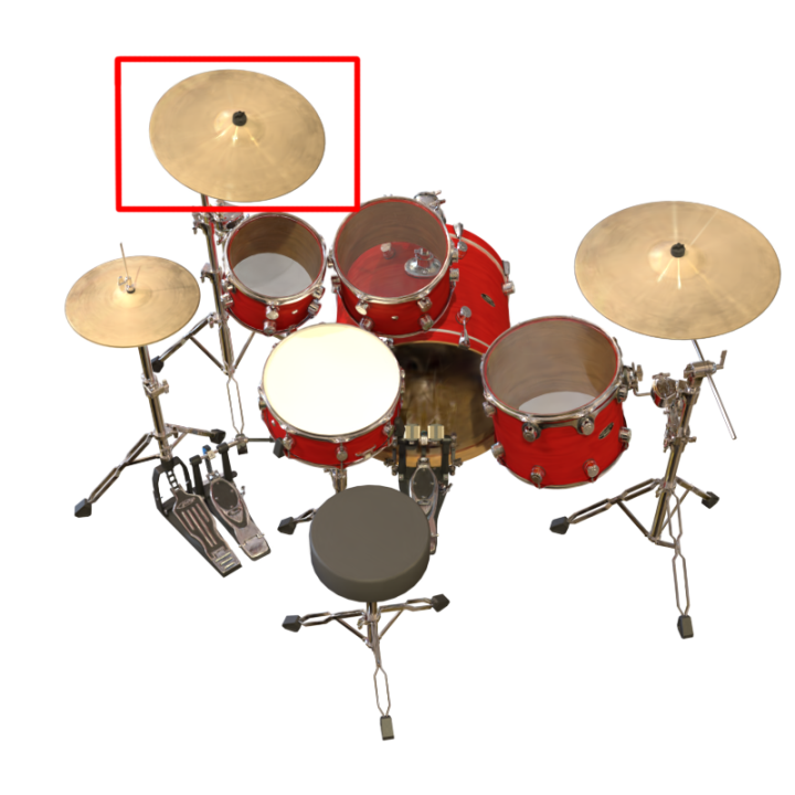
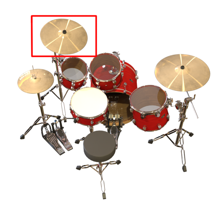
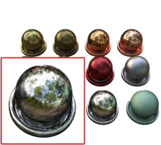
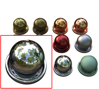
Figure 2: Visual comparison between classical GS and Viewing Direction Gaussian Splatting on the dataset: NeRF Synthetic (Mildenhall et al., 2020). As we can see, Viewing Direction Gaussian Splatting can better describe shadows, light reflection, and transparency of rendered 3D objects (see elements in red rectangles).

In NeRFs (Mildenhall et al., 2020), the scene is represented with the help of fully connected network architectures. These networks take as input 5D coordinates consisting of camera positions and spatial locations. From this data, they are able to generate the color and volume density of each point within the scene. The loss function of NeRF draws inspiration from conventional volume rendering techniques (Kajiya & Von Herzen, 1984), which involve rendering the color of every ray traversing the scene. In essence, NeRF embeds the shape and color information of the object within the neural network’s weights.

NeRF architecture excels at generating crisp renders of new viewpoints in static scenes. However, it faces several limitations, primarily stemming from the time-consuming process of encoding object shapes into neural network weights. In practice, training and inference with NeRF models can take extensive time, making them often impractical for real-time applications.

In comparison, Gaussian Splatting (GS) (Kerbl et al., 2023) provides a similar quality of renders with more rapid training and inference. This is a consequence of GS not requiring neural networks. Instead, we encode information about the 3D objects in a set of Gaussian distributions. These Gaussians can then be used in a similar manner to classical meshes. Consequently, GS can be swiftly developed when needed to, for example, model dynamic scenes (Wu et al., 2023). Unfortunately, GS is hard to condition as it necessitates a hundred thousand Gaussian components.

Both these rendering methods, i.e. NeRFs and SG, offer certain advantages and possess a range of caveats. In this paper, we present Viewing Direction Gaussian Splatting (VDGS), a new, hybrid approach that uses GS representation of the 3D object’s shape and simultaneously employs NeRF-based encoding of color and opacity. Our model uses Gaussian distributions with trainable positions (i.e., means of Gaussian), shape (i.e., covariance of Gaussian), color, and opacity, as well as a neural network, which takes a parameter of Gaussian together with viewing direction to produce changes in the color and opacity.

Such approaches inherit advantages of both NeRF and GS. First of all, Viewing Direction Gaussian Splatting has similar training and inference time as GS. Moreover, we can better model shadows, light reflection, and transparency in 3D objects by using viewing directions, see Fig. 1.

In summary, this work makes the following contributions:

• We propose a hybrid architecture utilizing both NeRF and GS. We encode the color and opacity using NeRF, whereas GS represents the 3D object’s shape. Therefore we inherit fast training and inference from GS and the ability to adapt to viewing direction from NeRF.

• In contrast to GS, in the VDGS color and opacity depend on viewing direction without causing a notable increase in training time.

• VDGS describe better shadows, light reflection, and transparency in 3D objects.

Gaussian Splatting   Viewing Direction Gaussian Splatting     Original image

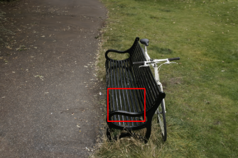
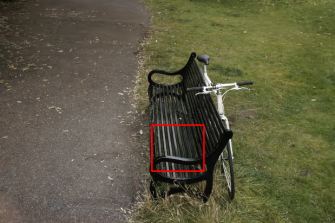
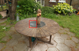
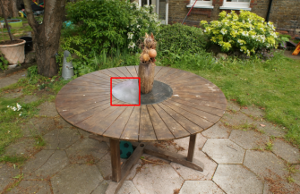
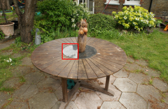
Figure 3: Visual comparison between classical GS and Viewing Direction Gaussian Splatting on three distinct datasets, namely, NeRF Synthetic (Mildenhall et al., 2020), Tanks and Temples (Knapitsch et al., 2017), and Shiny Blender (Verbin et al., 2022).

2 Related Works

We can rely on various techniques to represent 3D objects, including voxel grids (Choy et al., 2016), octrees (Häne et al., 2017), multi-view images (Arsalan Soltani et al., 2017), geometry images (Sinha et al., 2016), and finally, point clouds (Yang et al., 2022). An alternative approach is given through Neural Radiance Field (NeRF) (Mildenhall et al., 2020).

NeRF

The aforementioned representations are discrete, which can lead to issues in their applicability in various use case scenarios (Spurek et al., 2020). In comparison, NeRF (Mildenhall et al., 2020) utilizes a fully connected architecture to represent a scene. NeRF and its various generalizations (Barron et al., 2021, 2022; Liu et al., 2020; Niemeyer et al., 2022; Roessle et al., 2022; Tancik et al., 2022; Verbin et al., 2022) use differentiable volumetric rendering to generate novel views of a static scene.

The prolonged training time associated with traditional NeRFs has been tackled before with the introduction of Plenoxels (Fridovich-Keil et al., 2022). In this approach, we replace the dense voxel representation with a sparse voxel grid, significantly reducing the computational demands. Within this sparse grid, density and spherical harmonics coefficients are stored at each node, enabling the estimation of color based on trilinear interpolation of neighboring voxel values. On the other hand, Sun et al. (2022) delved into optimizing the features of voxel grids to achieve rapid radiance field reconstruction. Müller et al. (2022) refined this approach by partitioning the 3D space into independent multilevel grids to enhance its computational efficiency further. Chen et al. (2022) studies representation 3D object using orthogonal tensor components. A small MLP network extracts the final color and density from these components using orthogonal projection. Additionally, some methods use supplementary information like depth maps or point clouds (Azinović et al., 2022; Deng et al., 2022; Roessle et al., 2022). Zimny et al. (2023) proposed a MultiPlane version of NeRF with image-based planes to represent 3D objects. The TriPlane representation from EG3D (Chan et al., 2022) has a wide range of applications to diffusion-based generative model (Chen et al., 2023).

NeRF-based models can render highly sharp renders and be used in large generative models. Unfortunately, NeRF is expensive in training and rendering (Kerbl et al., 2023).

GS       VDGS     Original

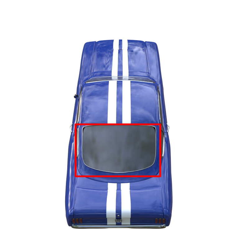
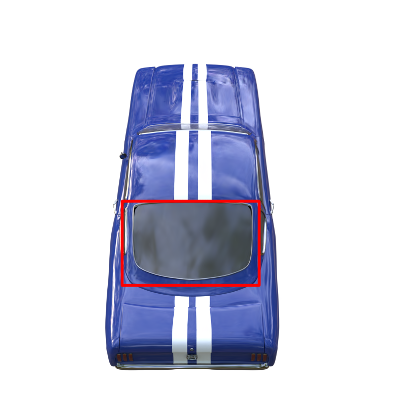
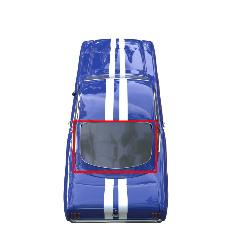
Figure 4: Visual comparison between classical GS and Viewing Direction Gaussian Splatting on the dataset: Shiny Blender (Verbin et al., 2022).

PSNR $\uparrow$
	Chair	Drums	Lego	Mic	Materials	Ship	Hotdog	Ficus	Avg.
NeRF	33.00	25.01	32.54	32.91	29.62	28.65	36.18	30.13	31.01
VolSDF	30.57	20.43	29.46	30.53	29.13	25.51	35.11	22.91	27.96
Ref-NeRF	33.98	25.43	35.10	33.65	27.10	29.24	37.04	28.74	31.29
ENVIDR	31.22	22.99	29.55	32.17	29.52	21.57	31.44	26.60	28.13
Gaussian Splatting	35.82	26.17	35.69	35.34	30.00	30.87	37.67	34.83	33.30
GaussianShader	35.83	26.36	35.87	35.23	30.07	30.82	37.85	34.97	33.38
VDGS (Our)	36.13	26.25	35.32	35.74	30.13	31.25	37.55	35.37	33.47
SSIM $\uparrow$
NeRF	0.967	0.925	0.961	0.980	0.949	0.856	0.974	0.964	0.947
VolSDF	0.949	0.893	0.951	0.969	0.954	0.842	0.972	0.929	0.932
Ref-NeRF	0.974	0.929	0.975	0.983	0.921	0.864	0.979	0.954	0.947
ENVIDR	0.976	0.930	0.961	0.984	0.968	0.855	0.963	0.987	0.956
Gaussian Splatting	0.987	0.954	0.983	0.991	0.960	0.907	0.985	0.987	0.969
GaussianShader	0.987	0.949	0.983	0.991	0.960	0.905	0.985	0.985	0.968
VDGS (Our)	0.987	0.952	0.980	0.992	0.962	0.907	0.984	0.988	0.969
LPIPS $\downarrow$
NeRF	0.046	0.091	0.050	0.028	0.063	0.206	0.121	0.044	0.081
VolSDF	0.056	0.119	0.054	0.191	0.048	0.191	0.043	0.068	0.096
Ref-NeRF	0.029	0.073	0.025	0.018	0.078	0.158	0.028	0.056	0.058
ENVIDR	0.031	0.080	0.054	0.021	0.045	0.228	0.072	0.010	0.067
Gaussian Splatting	0.012	0.037	0.016	0.006	0.034	0.106	0.020	0.012	0.030
GaussianShader	0.012	0.040	0.014	0.006	0.033	0.098	0.019	0.013	0.029
VDGS (Our)	0.013	0.039	0.018	0.006	0.034	0.108	0.022	0.010	0.031

Table 1: The quantitative comparisons (PSNR / SSIM / LPIPS) on NeRF Synthetic dataset.

Gaussian Splatting

The point-based representations such as Gaussian have been widely used in a variety of fields, including shape reconstruction (Keselman & Hebert, 2023), molecular structures modeling (Blinn, 1982), or the substitution of point-cloud data (Eckart et al., 2016). Moreover, these representations can be employed in shadow (Nulkar & Mueller, 2001) and cloud rendering applications (Man, 2006).

Recently, 3D Gaussian Splatting (3D-GS) (Kerbl et al., 2023), which combines the concept of point-based rendering and splatting techniques for rendering, has achieved real-time speed with a rendering quality that is comparable to the best MLP-based renderer, Mip-NeRF.

GS offers faster training and inference time than NeRF. Moreover, we do not use a neural network, as all the information is stored in 3D Gaussian components. Therefore, such a model finds application in dynamic scene modeling. Moreover, it is easy to combine with a dedicated 3D computer graphics engine (Kerbl et al., 2023). On the other hand, it is hard to condition GS since we typically have hundreds of thousands of Gaussian components.

In the paper, we present a fiction of NeRF model and GS representation of 3D objects.

3 Viewing Direction Gaussian Splatting

Here, we briefly describe the NeRF and GS models to better ground our findings. Next, we provide the details about Viewing Direction Gaussian Splatting, which is a hybrid of the above models.

NeRF representation of 3D objects

Vanilla NeRF (Mildenhall et al., 2020) represents geometrically-reach 3D scenes using neural model taking as an input a 5D coordinate composed of the viewing direction ${\bf d}=(\theta,\psi)$ and spatial location ${\bf x}=(x,y,z)$, that returns as its output emitted color ${\bf c}=(r,g,b)$ and volume density $\sigma$.

A vanilla NeRF employs a collection of images for training. This process entails generating an ensemble of rays that pass through the image and interact with a 3D object represented by a neural network. These interactions, including the observed color and depth, are then used to train the neural network to accurately represent the object’s shape and appearance. NeRF approximates this 3D object with an MLP network:

$$\mathcal{F}_{NeRF}({\bf x},{\bf d};\Theta)=({\bf c},\sigma).$$

The MLP parameters, $\bf\Theta$, are optimized during training to minimize the discrepancy between the rendered images and the reference images from a given dataset. Consequently, the MLP network takes a 3D coordinate as input and outputs a density value along with the radiance (color) in a specified direction.

The loss of NeRF is inspired by classical volume rendering (Kajiya & Von Herzen, 1984). We render the color of all rays traversing the scene. The volume density $\sigma({\bf x})$ can be interpreted as the differential probability of a ray. The expected color $C({\bf r})$ of camera ray ${\bf r}(t)={\bf o}+t{\bf d}$ (where ${\bf o}$ is ray origin and ${\bf d}$ is direction) can be computed with an integral, but in practice, it is estimated numerically using stratified sampling. The loss is simply the total squared error between the rendered and true pixel colors:

$$\mathcal{L}=\sum_{{\bf r}\in R}\|\hat{C}({\bf r})-C({\bf r})\|_{2}^{2},$$ (1)

where $R$ is the set of rays in each batch, and $C({\bf r})$, $\hat{C}({\bf r})$ are the ground truth and predicted RGB colors for ray r , respectively. The predicted RGB colors $\hat{C}({\bf r})$ can be obtained using the following equation:

$$\hat{C}({\bf r})=\sum_{i=1}^{N}T_{i}(1-\exp(-\sigma_{i}\delta_{i})){\bf c}_{i},$$ (2)

where $T_{i}=\exp\left(-\sum_{j=1}^{i-1}\sigma_{i}\delta_{i}\right)$ and $N$ is the number of samples, $\delta_{i}$ is the distance between adjacent samples, and $\sigma_{i}$ denotes the opacity of sample $i$. This function allowing computation of $\hat{C}({\bf r})$ from the set of $(c_{i},\sigma_{i})$ values is trivially differentiable.

	Mip-NeRF360			Tanks&Temples			Deep Blending
	SSIM $\uparrow$	PSNR $\uparrow$	LPIPS $\downarrow$	SSIM $\uparrow$	PSNR $\uparrow$	LPIPS $\downarrow$	SSIM $\uparrow$	PSNR $\uparrow$	LPIPS $\downarrow$
Plenoxels	0.626	23.08	0.719	0.379	21.08	0.795	0.510	23.06	0.510
INGP-Base	0.671	25.30	0.371	0.723	21.72	0.330	0.797	23.62	0.423
INGP-Big	0.699	25.59	0.331	0.745	21.92	0.305	0.817	24.96	0.390
M-NeRF360	0.792	27.69	0.237	0.759	22.22	0.257	0.901	29.40	0.245
Guassian Splatting-7K	0.770	25.60	0.279	0.767	21.20	0.280	0.875	27.78	0.317
Guassian Splatting-30K	0.815	27.21	0.214	0.841	23.14	0.183	0.903	29.41	0.243
VDGS (Our)	0.809	27.66	0.223	0.854	24.08	0.166	0.903	29.72	0.243

Table 2: Quantitative evaluation of Viewing Direction Gaussian Splatting method compared to previous work, computed over three distinct datasets, namely, NeRF synthetic (Mildenhall et al., 2020), Tanks and Temples (Knapitsch et al., 2017), and Shiny Blender (Verbin et al., 2022).

Synthetic NeRF
PSNR $\uparrow$
	Chair	Drums	Lego	Mic	Materials	Ship	Hotdog	Ficus	Avg.
GS	35.83	26.15	35.78	35.36	30.00	30.80	37.72	34.87	33.32
VDGS	36.13	26.25	35.32	35.74	30.13	31.23	37.55	35.37	33.47
Pre-train GS 30k + VDGS 20k	35.61	26.16	35.81	35.48	30.01	30.92	37.71	35.14	33.35

Mip-NeRF360
PSNR $\uparrow$
	Bicycle	Flowers	Garden	Stump	Treehill	Room	Counter	Kitchen	Bonsai	Avg.
GS	25.246	21.520	27.410	26.550	22.490	30.632	28.700	30.317	31.980	27.210
VDGS	25.127	21.259	27.645	26.515	22.774	31.523	29.650	31.600	32.894	27.665
Pre-train GS 30k + VDGS 20k	25.172	21.510	27.247	26.562	22.520	31.402	28.947	31.354	32.158	27.652

Table 3: Comparison between original GS model 30k epochs, VDGS 30k epochs and pre-trained GS standard model with additional 20k epochs with VDGS on synthetic NeRF data.

Such approaches to representing 3D objects using neural networks often face limitations due to their capacity or difficulty in precisely locating where camera rays intersect with the scene geometry. Consequently, generating high-resolution images from these representations often necessitates computationally expensive optical ray marching, hindering real-time use case scenarios.

Gaussian Splatting

Gaussian Splatting (GS) model 3D scene by a collection of 3D Gaussians defined by a position (mean), covariance matrix, opacity, and color represented via spherical harmonics (SH) (Fridovich-Keil et al., 2022; Müller et al., 2022).

GS algorithm creates the radiance field representation by a sequence of optimization steps of 3D Gaussian parameters (i.e., position, covariance, opacity, and SH colors). The key to the efficiency of GS is the rendering process, which uses projections of Gaussian components.

In GS, we use a dense set of 3D Gaussians:

$$\mathcal{G}=\{(\mathcal{N}(\mathrm{m}_{i},\Sigma_{i}),\sigma_{i},c_{i})\}_{i=1}^{n},$$

where $\mathrm{m}_{i}$ is position, $\Sigma_{i}$ is covariance, $\sigma_{i}$ is opacity, and $c$ is SH colors of $i$-th component.

GS optimization is based on a cycle of rendering and comparing the generated image to the training views in the collected data. Unfortunately, 3D to 2D projection can lead to incorrect geometry placement. Therefore, GS optimization must be able to create, destroy, and move geometry if it is incorrectly positioned. The quality of the parameters of the 3D Gaussian covariances is essential for the representation’s compactness, as large homogeneous areas can be captured with a small number of large anisotropic Gaussians.

GS starts with a limited number of points and then employs a strategy that involves creating new and eliminating unnecessary components. In practice, after every hundred iterations, GS eliminates any Gaussians with an opacity lower than a specific limit. At the same time, new Gaussians are generated in unoccupied areas of 3D space to fill vacant areas. The GS optimization process is complicated, but it can be trained very effectively thanks to robust implementation and the usage of CUDA kernels.

PSNR $\uparrow$
	Car	Ball	Helmet	Teapot	Toaster	Coffee	Avg.
NVDiffRec (Munkberg et al., 2022)	27.98	21.77	26.97	40.44	24.31	30.74	28.70
NVDiffMC (Hasselgren et al., 2022)	25.93	30.85	26.27	38.44	22.18	29.60	28.88
Ref-NeRF (Verbin et al., 2022)	30.41	29.14	29.92	45.19	25.29	33.99	32.32
NeRO (Liu et al., 2023)	25.53	30.26	29.20	38.70	26.46	28.89	29.84
ENVIDR (Liang et al., 2023)	28.46	38.89	32.73	41.59	26.11	29.48	32.88
Guassian Splatting (Kerbl et al., 2023)	27.24	27.69	28.32	45.68	20.99	32.32	30.37
GaussianShader (Jiang et al., 2023)	27.90	30.98	28.32	45.86	26.21	32.39	31.94
VDGS (Our)	26.99	27.87	28.18	45.39	21.53	32.16	30.35
SSIM $\uparrow$
NVDiffRec (Munkberg et al., 2022)	0.963	0.858	0.951	0.996	0.928	0.973	0.945
NVDiffMC (Hasselgren et al., 2022)	0.940	0.940	0.940	0.995	0.886	0.965	0.944
Ref-NeRF (Verbin et al., 2022)	0.949	0.956	0.955	0.995	0.910	0.972	0.956
NeRO (Liu et al., 2023)	0.949	0.974	0.971	0.995	0.929	0.956	0.962
ENVIDR (Liang et al., 2023)	0.961	0.991	0.980	0.996	0.939	0.949	0.969
Guassian Splatting (Kerbl et al., 2023)	0.930	0.937	0.951	0.996	0.895	0.971	0.947
GaussianShader (Jiang et al., 2023)	0.931	0.965	0.950	0.996	0.929	0.971	0.957
VDGS (Our)	0.938	0.944	0.949	0.996	0.899	0.971	0.949
LPIPS $\downarrow$
NVDiffRec (Munkberg et al., 2022)	0.045	0.297	0.118	0.011	0.169	0.076	0.119
NVDiffMC (Hasselgren et al., 2022)	0.077	0.312	0.157	0.014	0.225	0.097	0.147
Ref-NeRF (Verbin et al., 2022)	0.051	0.307	0.087	0.013	0.118	0.082	0.109
NeRO (Liu et al., 2023)	0.074	0.094	0.050	0.012	0.089	0.110	0.072
ENVIDR (Liang et al., 2023)	0.049	0.067	0.051	0.011	0.116	0.139	0.072
Guassian Splatting (Kerbl et al., 2023)	0.047	0.161	0.079	0.007	0.126	0.078	0.083
GaussianShader (Jiang et al., 2023)	0.045	0.121	0.076	0.007	0.079	0.078	0.068
VDGS (Our)	0.049	0.143	0.073	0.007	0.101	0.079	0.075

Table 4: The quantitative comparisons (PSNR / SSIM / LPIPS) on Shiny Blender dataset (Verbin et al., 2022).

Figure 5: In contrast to GS, where color and opacity are fixed, in Viewing Direction Gaussian Splatting color and opacity of Gaussians depend on the viewing direction. Consequently, we better model shadows, light reflection, and transparency of 3D objects (see elements in red rectangles).

Viewing Direction Gaussian Splatting

In our approach, we use GS to model 3D shapes, while a NeRF-based neural network produces colors and opacity. Our model consists of the following GS representation:

$$\mathcal{G}=\{(\mathcal{N}(\mathrm{m}_{i},\Sigma_{i}),\sigma_{i},c_{i})\}_{i=1}^{n},$$

and the MLP network:

$$\mathcal{F}_{VDGS{}}(\Sigma,c,{\bf d};\Theta)=\Delta\sigma({\bf d}),$$

which takes selected parameters of Gaussian distribution and viewing direction ${\bf d}$ to returns volume density update $\Delta\sigma({\bf d})$. The model is parameterized by $\bf\Theta$ and trained to change color and opacity depending on viewing direction.

The final VDGS model is given by:

$$(\mathcal{G},\mathcal{F}_{VDGS{}})=\{(\mathcal{N}(\mathrm{m}_{i},\Sigma_{i}),\sigma_{i}\cdot\Delta\sigma_{i}({\bf d}),{\bf c_{i}})\}_{i=1}^{n},$$

where

$$\Delta\sigma_{i}({\bf d})=\mathcal{F}_{VDGS{}}(\Sigma_{i},c_{i},{\bf d}).$$

Consequently, we have two components, i.e., GS and NeRF. The former is used to produce the 3D object’s shape and color. All Gaussian components have color and transparent transparency value, which do not depend on viewing direction. Thanks to GS, we model the universal colors, which do not depend on the viewing direction. In addition, the NeRF component can add minor transparency changes to the objects depending on the camera position, see Fig. 5. As a consequence, our model can add viewing direction-based changes. Therefore, it allows the modeling of light reflection and transparency of the objects.

Updates in Viewing Direction Gaussian Splatting

In our main model, we use updates only to the transparency of Gaussian components. In practice, we can also modify color. Moreover, we can model updates not multiplicatively but by classical sum. In the next section with our experimental results, we evaluate the following models:

• VDGS Color Add model is given by:
  $(\mathcal{G},\mathcal{F}_{VDGS{}})\!\!=\!\!\{(\mathcal{N}(\mathrm{m}_{i},\Sigma_{i}),\sigma_{i},{\bf c_{i}}+{\bf\Delta c_{i}}({\bf d}))\}_{i},$

• VDGS Color Multiply is given by:
  $(\mathcal{G},\mathcal{F}_{VDGS{}})\!\!=\!\!\{(\mathcal{N}(\mathrm{m}_{i},\Sigma_{i}),\sigma_{i},{\bf c_{i}}*{\bf\Delta c_{i}}({\bf d}))\}_{i},$

• VDGS Opacity Add is given by:
  $(\mathcal{G},\mathcal{F}_{VDGS{}})\!\!=\!\!\{(\mathcal{N}(\mathrm{m}_{i},\Sigma_{i}),\sigma_{i}+\Delta\sigma_{i}({\bf d}),{\bf c_{i}})\}_{i},$

• VDGS Opacity Multiply is given by:
  $(\mathcal{G},\mathcal{F}_{VDGS{}})\!\!=\!\!\{(\mathcal{N}(\mathrm{m}_{i},\Sigma_{i}),\sigma_{i}*\Delta\sigma_{i}({\bf d}),{\bf c_{i}})\}_{i},$

• VDGS Opacity and Color Add is given by:
  $(\mathcal{G},\mathcal{F}_{VDGS{}})\!\!=\!\!\{(\mathcal{N}(\mathrm{m}_{i},\Sigma_{i}),\sigma_{i}\!+\!\Delta\sigma_{i}({\bf d}),{\bf c_{i}}\!+\!{\bf\Delta c_{i}})\}_{i},$

• VDGS Opacity and Color Multiply is given by:
  $(\mathcal{G},\mathcal{F}_{VDGS{}})\!\!=\!\!\{(\mathcal{N}(\mathrm{m}_{i},\Sigma_{i}),\sigma_{i}\!*\!\Delta\sigma_{i}({\bf d}),{\bf c_{i}}\!*\!{\bf\Delta c_{i}})\}_{i},$

The results of our experiments show that all approaches have some advantages and obtain good results for different scoring functions. In practice, we select the model that gives the best PSNR scores. The PSNR is the most popular evaluation function.

	Mip-NeRF360		Tanks&Temples		Deep Blending
	Train	FPS	Train	FPS	Train	FPS
Plenoxels	25m49s	6.79	25m5s	13.0	27m49s	11.2
INGP-Base	5m37s	11.7	5m26s	17.1	6m31s	3.26
INGP-Big	7m30s	9.43	6m59s	14.4	8m	2.79
M-NeRF360	48h	0.06	48h	0.14	48h	0.09
GS-30K	41m33s	134	26m54s	154	36m2s	137
GS-30K*	26m4s	92.44	14m35s	93.49	23m45s	86.80
VDGS-30K*	55m32s	29.25	36m26s	27.41	48m4s	31.53

Table 5: Comparison of training time and frame rate. We train VDGS on the RTX 3090 GPU. *We reproduce the result of GS on the RTX 3090 GPU. VDGS has slightly longer training and inference time.

4 Experiments

Datasets

To comprehensively validate the effectiveness of VDGS, we conducted an evaluation on various datasets: a) widely-used NVS dataset, i.e., the NeRF Synthetic (Mildenhall et al., 2020), b) real-world, large-scale scenes dataset, i.e., the Tanks and Temples (Knapitsch et al., 2017), and c) reflective objects datasets, i.e., the Shiny Blender (Verbin et al., 2022).

PSNR $\uparrow$
	Others		NeRF Synthetic
VDGS	Tanks	Blending	Chair	Drums	Lego	Mic	Materials	Ship	Hotdog	Ficus	Avg.
Color Add	23.79	29.20	35.72	26.66	35.95	35.41	30.07	30.98	37.99	35.25	33.50
Color Multiply	23.69	29.33	35.97	26.34	35.79	35.47	30.01	30.98	37.86	34.99	33.42
Opacity Add	22.86	14.89	34.93	25.42	28.51	34.48	27.26	23.74	33.22	33.89	30.18
Opacity Multiply	24.08	29.72	36.13	26.25	35.32	35.74	30.13	31.25	37.55	35.37	33.47
Opacity and Color Add	23.33	29.06	35.45	26.21	31.81	35.73	29.59	28.57	35.90	34.91	32.27
Opacity and Color Multiply	23.76	29.65	36.16	24.40	35.51	13.03	8.73	31.15	37.74	14.21	25.37

PSNR $\uparrow$
Mip-NeRF360
VDGS	Bicycle	Flowers	Garden	Stump	Treehill	Room	Counter	Kitchen	Bonsai
Color Add	24.99	21.28	27.26	26.37	22.49	31.31	29.28	31.51	32.32
Color Multiply	25.21	21.47	27.40	26.71	22.60	31.40	29.07	31.57	32.28
Opacity Add	24.56	20.56	26.42	25.95	19.27	29.53	27.90	29.44	29.44
Opacity Multiply	25.13	21.26	27.65	26.52	22.77	31.52	29.65	31.60	32.89
Opacity and Color Add	24.89	20.86	25.26	26.14	21.15	29.81	27.89	28.17	29.20
Opacity and Color Multiply	25.27	21.34	27.54	26.35	22.76	31.42	29.37	31.28	32.32

Table 6: Ablation study of different versions of Viewing Direction Gaussian Splatting. As we can see, different versions considered have good scores in various data sets and measures. In our paper, we chose VDGS Opacity Multiply (Our) as a final model, since we obtained the largest number of best scores on the PSNR measure.

Dataset: NeRF Synthetic

We first evaluate our model on the NeRF Synthetic dataset (Mildenhall et al., 2020), which contains objects with complex geometry and realistic non-Lambertian materials. We show the quantitative results in Tab. 1 and visual comparisons in Fig. 2. The results show that our approach achieved better results than both GS and neural rendering methods.

Dataset: Tanks and Temples

We evaluated our model on larger-scale environments by comparing our solution on the Tanks and Temples dataset (Knapitsch et al., 2017). Tab. 2 and visual comparisons in Fig. 3 show that we can better model light reflexes and shadows than either GS or NeRF. Our model obtained the best score in most datasets and measures.

Dataset: Shiny Blender

Viewing Direction Gaussian Splatting can plausible model shadows, light reflection, and transparency in 3D objects. Therefore, we decided to evaluate our hybrid approach on the Shiny Blender dataset (Verbin et al., 2022). Once again, visual comparisons in Fig. 4 and quantitative results in Tab. 4 show that we obtain comparable results to NeRF and GS approaches but slightly worse than the dedicated method GaussianShader (Jiang et al., 2023).

Pre-trained GS

Our model simultanesly train GS and NeRF component. In Tab. 3 we present results on pre-train GS model. We use fully train GS model, and than we tune our neural network. As we can see such approche gives better results than vanila GS. On the other hand when we trin both components we obtin the best scores.

Training and inference time

In contrast to GS in VDGS we use a viewing direction neural network. Therefore we have slightly longer training and inference time, see Tab. 5. In practice, our model can work in real-time during inference.

Ablation Study

Our VDGS uses change only in opacity. It is a natural question of how our model works when also color is changing. In the ablation study, we verify different versions of Viewing Direction Gaussian Splatting. In Tab. 6, we present the PSNR value for a different version of our model. In the appendix, we present full results on PSNR/SSIM/LPIPS measures.

As we can see, different versions of Viewing Direction Gaussian Splatting result in high scores for various data sets. In our paper, we chose VDGS Opacity Multiply as a final model since we obtained the largest number of best scores on the PSNR measure on the data containing real scenes. It also should be highlighted that model VDGS Color Multiply gets the best scores on the NeRF Synthetic dataset.

Models that use both color and opacity also obtain good results but are slightly worse than model which uses only one of such elements. We believe this effect may be attributed to the dependency of opacity on color. Therefore, joint training is not effective.

5 Conclusions

This paper presents a new neural rendering strategy that leverages two main concepts, NeRF and GS. We represent a 3D scene with a set of Gaussian components and a neural network that can change the color and opacity of Gaussians concerning viewing direction. This approach inherited the best elements from the NeRF and GS methods. We observed swift training and inference, and we can effectively model shadows, light reflections, and transparency for generating plausible 3D objects. Furthermore, the conduced experiments show that Viewing Direction Gaussian Splatting gives better results than NeRF as well as the GS model.

6 Appendix

Updates in Viewing Direction Gaussian Splatting

In our main model, we use updates only to the transparency of Gaussian components. In practice, we can also modify color. Moreover, we can model updates not multiplicatively but by classical sum. In the next section with our experimental results, we evaluate the following models:

• VDGS Color Add model is given by:
  $(\mathcal{G},\mathcal{F}_{VDGS{}})\!\!=\!\!\{(\mathcal{N}(\mathrm{m}_{i},\Sigma_{i}),\sigma_{i},{\bf c_{i}}+{\bf\Delta c_{i}}({\bf d}))\}_{i},$

• VDGS Color Multiply is given by:
  $(\mathcal{G},\mathcal{F}_{VDGS{}})\!\!=\!\!\{(\mathcal{N}(\mathrm{m}_{i},\Sigma_{i}),\sigma_{i},{\bf c_{i}}*{\bf\Delta c_{i}}({\bf d}))\}_{i},$

• VDGS Opacity Add is given by:
  $(\mathcal{G},\mathcal{F}_{VDGS{}})\!\!=\!\!\{(\mathcal{N}(\mathrm{m}_{i},\Sigma_{i}),\sigma_{i}+\Delta\sigma_{i}({\bf d}),{\bf c_{i}})\}_{i},$

• VDGS Opacity Multiply is given by:
  $(\mathcal{G},\mathcal{F}_{VDGS{}})\!\!=\!\!\{(\mathcal{N}(\mathrm{m}_{i},\Sigma_{i}),\sigma_{i}*\Delta\sigma_{i}({\bf d}),{\bf c_{i}})\}_{i},$

• VDGS Opacity and Color Add is given by:
  $(\mathcal{G},\mathcal{F}_{VDGS{}})\!\!=\!\!\{(\mathcal{N}(\mathrm{m}_{i},\Sigma_{i}),\sigma_{i}\!+\!\Delta\sigma_{i}({\bf d}),{\bf c_{i}}\!+\!{\bf\Delta c_{i}})\}_{i},$

• VDGS Opacity and Color Multiply is given by:
  $(\mathcal{G},\mathcal{F}_{VDGS{}})\!\!=\!\!\{(\mathcal{N}(\mathrm{m}_{i},\Sigma_{i}),\sigma_{i}\!*\!\Delta\sigma_{i}({\bf d}),{\bf c_{i}}\!*\!{\bf\Delta c_{i}})\}_{i},$

In Tab. 7, 8, 9 we present extension of experimented from main paper. In tables we show average SSIM, PSNR and LPIPS results for each of datasets-Mip-NeRF360, Tanks&Temples as well as Deep Blending. We also include detailed information about PSNR, SSIM and LPIPS results for each object in Synthetic and Shiny datasets using different types of VDGS model. Tab. 10 includes detailed information about PSNR, SSIM and LPIPS for every scene in Mip-NeRF360 (first part of the table from bicycle to bonsai), Tanks&Temples (truck and train) and Deep Blending (drjohnson and playroom).

	Mip-NeRF360			Tanks&Temples			Deep Blending
	SSIM $\uparrow$	PSNR $\uparrow$	LPIPS $\downarrow$	SSIM $\uparrow$	PSNR $\uparrow$	LPIPS $\downarrow$	SSIM $\uparrow$	PSNR $\uparrow$	LPIPS $\downarrow$
Color Add	0.811	27.42	0.217	0.850	23.79	0.172	0.898	29.20	0.249
Color Multiply	0.815	27.52	0.215	0.848	23.69	0.174	0.899	29.33	0.248
Opacity Add	0.773	25.90	0.279	0.808	22.86	0.245	0.420	14.89	0.490
Opacity Multiply	0.813	27.66	0.220	0.845	24.08	0.174	0.900	29.91	0.242
Opacity and Color Add	0.779	25.92	0.271	0.825	23.33	0.221	0.898	29.06	0.266
Opacity and Color Multiply	0.810	27.51	0.220	0.851	23.76	0.176	0.904	29.65	0.244

Table 7: Quantitative evaluation of Viewing Direction Gaussian Splatting method compared to previous work, computed over three distinct datasets, namely, NeRF synthetic (Mildenhall et al., 2020), Tanks and Temples (Knapitsch et al., 2017), and Shiny Blender (Verbin et al., 2022).

PSNR $\uparrow$
	Chair	Drums	Lego	Mic	Materials	Ship	Hotdog	Ficus	Avg.
Color Add	35.72	26.66	35.95	35.41	30.07	30.98	37.99	35.25	33.50
Color Multiply	35.97	26.34	35.79	35.47	30.01	30.98	37.86	34.99	33.42
Opacity Add	34.93	25.42	28.51	34.48	27.26	23.74	33.22	33.89	30.18
Opacity Multiply	36.13	26.25	35.32	35.74	30.13	31.25	37.55	35.37	33.47
Opacity and Color Add	35.45	26.21	31.81	35.73	29.59	28.57	35.90	34.91	32.27
Opacity and Color Multiply	36.16	24.40	35.51	13.03	8.73	31.15	37.74	14.21	25.37
SSIM $\uparrow$
Color Add	0.988	0.955	0.983	0.992	0.961	0.907	0.985	0.988	0.970
Color Multiply	0.987	0.955	0.983	0.991	0.961	0.907	0.985	0.988	0.969
Opacity Add	0.982	0.941	0.938	0.989	0.940	0.815	0.967	0.984	0.944
Opacity Multiply	0.987	0.952	0.980	0.992	0.962	0.907	0.984	0.988	0.969
Opacity and Color Add	0.985	0.950	0.965	0.991	0.956	0.864	0.978	0.988	0.959
Opacity and Color Multiply	0.987	0.952	0.981	0.884	0.771	0.907	0.984	0.857	0.915
LPIPS $\downarrow$
Color Add	0.012	0.036	0.015	0.006	0.034	0.104	0.020	0.011	0.029
Color Multiply	0.012	0.038	0.016	0.006	0.035	0.107	0.020	0.012	0.030
Opacity Add	0.016	0.049	0.060	0.008	0.053	0.233	0.048	0.014	0.060
Opacity Multiply	0.013	0.039	0.018	0.006	0.034	0.108	0.022	0.010	0.031
Opacity and Color Add	0.013	0.040	0.033	0.007	0.041	0.146	0.032	0.011	0.040
Opacity and Color Multiply	0.012	0.038	0.017	0.141	0.240	0.107	0.021	0.014	0.090

Table 8: The quantitative comparisons (PSNR / SSIM / LPIPS) on NeRF Synthetic dataset.

PSNR $\uparrow$
	Car	Ball	Helmet	Teapot	Toaster	Coffee	Avg.
Color Add	27.37	27.55	28.47	45.18	22.22	32.15	30.49
Color Multiply	27.50	27.89	28.15	45.81	21.35	32.50	30.53
Opacity Add	24.68	26.36	26.50	17.83	21.19	28.58	24.19
Opacity Multiply	26.99	27.87	28.18	45.39	21.53	32.16	30.35
Opacity and Color Add	27.06	27.57	27.88	44.37	22.25	31.21	30.07
Opacity and Color Multiply	27.04	27.69	28.83	45.79	21.73	32.16	30.54
SSIM $\uparrow$
Color Add	0.930	0.938	0.951	0.996	0.904	0.971	0.948
Color Multiply	0.932	0.938	0.951	0.997	0.899	0.972	0.948
Opacity Add	0.906	0.932	0.939	0.968	0.883	0.955	0.931
Opacity Multiply	0.938	0.944	0.949	0.996	0.899	0.971	0.949
Opacity and Color Add	0.928	0.944	0.949	0.996	0.905	0.968	0.948
Opacity and Color Multiply	0.928	0.942	0.950	0.996	0.902	0.971	0.948
LPIPS $\downarrow$
Color Add	0.046	0.160	0.075	0.008	0.106	0.078	0.078
Color Multiply	0.047	0.161	0.079	0.007	0.124	0.078	0.082
Opacity Add	0.073	0.163	0.089	0.079	0.119	0.103	0.104
Opacity Multiply	0.049	0.143	0.073	0.007	0.101	0.079	0.075
Opacity and Color Add	0.050	0.149	0.077	0.009	0.097	0.086	0.078
Opacity and Color Multiply	0.048	0.144	0.071	0.006	0.097	0.078	0.074

Table 9: Ablation study of different versions of Viewing Direction Gaussian Splatting. As we can see, different versions considered have good scores in various data sets and measures. In our paper, we chose VDGS Opacity Multiply as a final model, since we obtained the largest number of best scores on the PSNR measure.

PSNR $\uparrow$
	bicycle	flowers	garden	stump	treehill	room	counter	kitchen	bonsai
Color Add	24.99	21.28	27.26	26.37	22.49	31.31	29.28	31.51	32.32
Color Multiply	25.21	21.47	27.40	26.71	22.60	31.40	29.07	31.57	32.28
Opacity Add	24.56	20.56	26.42	25.95	19.27	29.53	27.90	29.44	29.44
Opacity Multiply	25.13	21.26	27.65	26.52	22.77	31.52	29.65	31.60	32.89
Opacity and Color Add	24.89	20.86	25.26	26.14	21.15	29.81	27.89	28.17	29.20
Opacity and Color Multiply	25.27	21.34	27.54	26.35	22.76	31.42	29.37	31.28	32.32
SSIM $\uparrow$
Color Add	0.757	0.599	0.863	0.762	0.632	0.916	0.907	0.926	0.940
Color Multiply	0.765	0.602	0.864	0.774	0.637	0.918	0.907	0.926	0.940
Opacity Add	0.757	0.596	0.865	0.768	0.636	0.916	0.910	0.926	0.942
Opacity Multiply	0.723	0.558	0.814	0.739	0.557	0.888	0.873	0.892	0.916
Opacity and Color Add	0.741	0.575	0.782	0.751	0.597	0.895	0.880	0.870	0.918
Opacity and Color Multiply	0.764	0.598	0.866	0.771	0.641	0.918	0.909	0.925	0.938
LPIPS $\downarrow$
Color Add	0.215	0.342	0.106	0.219	0.324	0.221	0.200	0.126	0.204
Color Multiply	0.208	0.338	0.105	0.212	0.322	0.218	0.199	0.125	0.204
Opacity Add	0.232	0.345	0.108	0.220	0.330	0.218	0.200	0.126	0.204
Opacity Multiply	0.274	0.382	0.173	0.271	0.417	0.288	0.262	0.190	0.251
Opacity and Color Add	0.258	0.372	0.188	0.261	0.387	0.269	0.249	0.206	0.246
Opacity and Color Multiply	0.227	0.346	0.105	0.219	0.325	0.219	0.201	0.127	0.209

PSNR $\uparrow$
	truck	train	drjohnson	playroom
Color Add	25.39	22.18	28.84	29.55
Color Multiply	25.37	22.01	29.04	29.62
Opacity Add	24.02	21.70	8.47	21.30
Opacity Multiply	25.70	22.46	29.42	30.02
Opacity and Color Add	24.67	21.99	29.46	28.64
Opacity and Color Multiply	25.44	22.09	29.51	29.77
SSIM $\uparrow$
Color Add	0.879	0.821	0.896	0.900
Color Multiply	0.878	0.819	0.896	0.901
Opacity Add	0.826	0.789	0.013	0.836
Opacity Multiply	0.880	0.810	0.900	0.900
Opacity and Color Add	0.853	0.797	0.903	0.892
Opacity and Color Multiply	0.881	0.820	0.904	0.904
LPIPS $\downarrow$
Color Add	0.147	0.197	0.249	0.249
Color Multiply	0.147	0.200	0.247	0.249
Opacity Add	0.237	0.252	0.612	0.361
Opacity Multiply	0.140	0.208	0.240	0.244
Opacity and Color Add	0.196	0.246	0.256	0.275
Opacity and Color Multiply	0.147	0.204	0.243	0.244

Table 10: Detailed results for ablation study of different versions of Viewing Direction Gaussian Splatting for Mip-NeRF360, Tanks&Temples and Deep Blending datasets.

References

- Arsalan Soltani et al. (2017) Arsalan Soltani, A., Huang, H., Wu, J., Kulkarni, T. D., and Tenenbaum, J. B. Synthesizing 3d shapes via modeling multi-view depth maps and silhouettes with deep generative networks. In Proceedings of the IEEE conference on computer vision and pattern recognition, pp. 1511–1519, 2017.
- Azinović et al. (2022) Azinović, D., Martin-Brualla, R., Goldman, D. B., Nießner, M., and Thies, J. Neural rgb-d surface reconstruction. In Proceedings of the IEEE/CVF Conference on Computer Vision and Pattern Recognition, pp. 6290–6301, 2022.
- Barron et al. (2021) Barron, J. T., Mildenhall, B., Tancik, M., Hedman, P., Martin-Brualla, R., and Srinivasan, P. P. Mip-nerf: A multiscale representation for anti-aliasing neural radiance fields. In Proceedings of the IEEE/CVF International Conference on Computer Vision, pp. 5855–5864, 2021.
- Barron et al. (2022) Barron, J. T., Mildenhall, B., Verbin, D., Srinivasan, P. P., and Hedman, P. Mip-nerf 360: Unbounded anti-aliased neural radiance fields. In Proceedings of the IEEE/CVF Conference on Computer Vision and Pattern Recognition, pp. 5470–5479, 2022.
- Blinn (1982) Blinn, J. F. A generalization of algebraic surface drawing. ACM transactions on graphics (TOG), 1(3):235–256, 1982.
- Chan et al. (2022) Chan, E. R., Lin, C. Z., Chan, M. A., Nagano, K., Pan, B., De Mello, S., Gallo, O., Guibas, L. J., Tremblay, J., Khamis, S., et al. Efficient geometry-aware 3d generative adversarial networks. In Proceedings of the IEEE/CVF Conference on Computer Vision and Pattern Recognition, pp. 16123–16133, 2022.
- Chen et al. (2022) Chen, A., Xu, Z., Geiger, A., Yu, J., and Su, H. Tensorf: Tensorial radiance fields. In Computer Vision–ECCV 2022: 17th European Conference, Tel Aviv, Israel, October 23–27, 2022, Proceedings, Part XXXII, pp. 333–350. Springer, 2022.
- Chen et al. (2023) Chen, H., Gu, J., Chen, A., Tian, W., Tu, Z., Liu, L., and Su, H. Single-stage diffusion nerf: A unified approach to 3d generation and reconstruction. In ICCV, 2023.
- Choy et al. (2016) Choy, C. B., Xu, D., Gwak, J., Chen, K., and Savarese, S. 3d-r2n2: A unified approach for single and multi-view 3d object reconstruction. In European conference on computer vision, pp. 628–644. Springer, 2016.
- Deng et al. (2022) Deng, K., Liu, A., Zhu, J.-Y., and Ramanan, D. Depth-supervised nerf: Fewer views and faster training for free. In Proceedings of the IEEE/CVF Conference on Computer Vision and Pattern Recognition, pp. 12882–12891, 2022.
- Eckart et al. (2016) Eckart, B., Kim, K., Troccoli, A., Kelly, A., and Kautz, J. Accelerated generative models for 3d point cloud data. In Proceedings of the IEEE conference on computer vision and pattern recognition, pp. 5497–5505, 2016.
- Fridovich-Keil et al. (2022) Fridovich-Keil, S., Yu, A., Tancik, M., Chen, Q., Recht, B., and Kanazawa, A. Plenoxels: Radiance fields without neural networks. In CVPR, pp. 5501–5510, 2022.
- Häne et al. (2017) Häne, C., Tulsiani, S., and Malik, J. Hierarchical surface prediction for 3d object reconstruction. In 2017 International Conference on 3D Vision (3DV), pp. 412–420. IEEE, 2017.
- Hasselgren et al. (2022) Hasselgren, J., Hofmann, N., and Munkberg, J. Shape, light, and material decomposition from images using monte carlo rendering and denoising. Advances in Neural Information Processing Systems, 35:22856–22869, 2022.
- Jiang et al. (2023) Jiang, Y., Tu, J., Liu, Y., Gao, X., Long, X., Wang, W., and Ma, Y. Gaussianshader: 3d gaussian splatting with shading functions for reflective surfaces. arXiv preprint arXiv:2311.17977, 2023.
- Kajiya & Von Herzen (1984) Kajiya, J. T. and Von Herzen, B. P. Ray tracing volume densities. ACM SIGGRAPH computer graphics, 18(3):165–174, 1984.
- Kerbl et al. (2023) Kerbl, B., Kopanas, G., Leimkühler, T., and Drettakis, G. 3d gaussian splatting for real-time radiance field rendering. ACM Transactions on Graphics, 42(4), 2023.
- Keselman & Hebert (2023) Keselman, L. and Hebert, M. Flexible techniques for differentiable rendering with 3d gaussians. arXiv preprint arXiv:2308.14737, 2023.
- Knapitsch et al. (2017) Knapitsch, A., Park, J., Zhou, Q.-Y., and Koltun, V. Tanks and temples: Benchmarking large-scale scene reconstruction. ACM Transactions on Graphics (ToG), 36(4):1–13, 2017.
- Liang et al. (2023) Liang, R., Chen, H., Li, C., Chen, F., Panneer, S., and Vijaykumar, N. Envidr: Implicit differentiable renderer with neural environment lighting. arXiv preprint arXiv:2303.13022, 2023.
- Liu et al. (2020) Liu, L., Gu, J., Zaw Lin, K., Chua, T.-S., and Theobalt, C. Neural sparse voxel fields. Advances in Neural Information Processing Systems, 33:15651–15663, 2020.
- Liu et al. (2023) Liu, Y., Wang, P., Lin, C., Long, X., Wang, J., Liu, L., Komura, T., and Wang, W. Nero: Neural geometry and brdf reconstruction of reflective objects from multiview images. arXiv preprint arXiv:2305.17398, 2023.
- Man (2006) Man, P. Generating and real-time rendering of clouds. In Central European seminar on computer graphics, volume 1. Citeseer Castá-Papiernicka, Slovakia, 2006.
- Mildenhall et al. (2020) Mildenhall, B., Srinivasan, P. P., Tancik, M., Barron, J. T., Ramamoorthi, R., and Ng, R. Nerf: Representing scenes as neural radiance fields for view synthesis. In ECCV, 2020.
- Müller et al. (2022) Müller, T., Evans, A., Schied, C., and Keller, A. Instant neural graphics primitives with a multiresolution hash encoding. ACM Transactions on Graphics (ToG), 41(4):1–15, 2022.
- Munkberg et al. (2022) Munkberg, J., Hasselgren, J., Shen, T., Gao, J., Chen, W., Evans, A., Müller, T., and Fidler, S. Extracting triangular 3d models, materials, and lighting from images. In Proceedings of the IEEE/CVF Conference on Computer Vision and Pattern Recognition, pp. 8280–8290, 2022.
- Niemeyer et al. (2022) Niemeyer, M., Barron, J. T., Mildenhall, B., Sajjadi, M. S., Geiger, A., and Radwan, N. Regnerf: Regularizing neural radiance fields for view synthesis from sparse inputs. In Proceedings of the IEEE/CVF Conference on Computer Vision and Pattern Recognition, pp. 5480–5490, 2022.
- Nulkar & Mueller (2001) Nulkar, M. and Mueller, K. Splatting with shadows. In Volume Graphics 2001: Proceedings of the Joint IEEE TCVG and Eurographics Workshop in Stony Brook, New York, USA, June 21–22, 2001, pp. 35–49. Springer, 2001.
- Roessle et al. (2022) Roessle, B., Barron, J. T., Mildenhall, B., Srinivasan, P. P., and Nießner, M. Dense depth priors for neural radiance fields from sparse input views. In Proceedings of the IEEE/CVF Conference on Computer Vision and Pattern Recognition, pp. 12892–12901, 2022.
- Sinha et al. (2016) Sinha, A., Bai, J., and Ramani, K. Deep learning 3d shape surfaces using geometry images. In European Conference on Computer Vision, pp. 223–240. Springer, 2016.
- Spurek et al. (2020) Spurek, P., Winczowski, S., Tabor, J., Zamorski, M., Zieba, M., and Trzciński, T. Hypernetwork approach to generating point clouds. Proceedings of Machine Learning Research, 119, 2020.
- Sun et al. (2022) Sun, C., Sun, M., and Chen, H.-T. Direct voxel grid optimization: Super-fast convergence for radiance fields reconstruction. In CVPR, pp. 5459–5469, 2022.
- Tancik et al. (2022) Tancik, M., Casser, V., Yan, X., Pradhan, S., Mildenhall, B., Srinivasan, P. P., Barron, J. T., and Kretzschmar, H. Block-nerf: Scalable large scene neural view synthesis. In Proceedings of the IEEE/CVF Conference on Computer Vision and Pattern Recognition, pp. 8248–8258, 2022.
- Verbin et al. (2022) Verbin, D., Hedman, P., Mildenhall, B., Zickler, T., Barron, J. T., and Srinivasan, P. P. Ref-nerf: Structured view-dependent appearance for neural radiance fields. In 2022 IEEE/CVF Conference on Computer Vision and Pattern Recognition (CVPR), pp. 5481–5490. IEEE, 2022.
- Wu et al. (2023) Wu, G., Yi, T., Fang, J., Xie, L., Zhang, X., Wei, W., Liu, W., Tian, Q., and Wang, X. 4d gaussian splatting for real-time dynamic scene rendering. arXiv preprint arXiv:2310.08528, 2023.
- Yang et al. (2022) Yang, F., Davoine, F., Wang, H., and Jin, Z. Continuous conditional random field convolution for point cloud segmentation. Pattern Recognition, 122:108357, 2022.
- Zimny et al. (2023) Zimny, D., Tabor, J., Zięba, M., and Spurek, P. Multiplanenerf: Neural radiance field with non-trainable representation. arXiv preprint arXiv:2305.10579, 2023.