Thermodynamics and Holography of Three-dimensional Accelerating black holes

Abstract

We address the problem of describing the thermodynamics and holography of three-dimensional accelerating black holes. By embedding the solutions in the Chern-Simons formalism, we identify two distinct masses, each with its associated first law of thermodynamics. We also show that a boundary entropy should be included (or excluded) in the black hole entropy.

¹State Key Laboratory of Quantum Optics and Quantum Optics Devices, Institute of Theoretical Physics, Shanxi University, Taiyuan 030006, P. R. China
²Kavli Institute for Theoretical Sciences (KITS),
University of Chinese Academy of Science, 100190 Beijing, P. R. China
³School of Physical Sciences, University of Chinese Academy of Sciences, Zhongguancun East Road 80, Beijing 100190, P. R. China

1 Introduction

Black holes play pivotal roles in general relativity, quantum gravity, and AdS/CFT holography [1, 2, 3]. An intriguing category is the accelerating black hole. Its exact solution existed solely in four-dimensional (4D) spacetime, termed the C-metric, until recently when 3D C-metrics describing compact accelerating black holes were introduced in [4, 5]. 4D C-metrics have been scrutinized in many aspects [6, 7, 8, 9, 10, 11, 12, 13, 14, 15, 16, 17, 18, 19, 20, 21, 22, 23, 24, 25, 26, 27, 28, 29, 30, 31, 32, 33, 34, 35, 36, 37, 38, 39, 40, 41]. However, the 3D C-metric which is supposed to be a simpler playground for holographic exploration proves more enigmatic [42, 43, 4, 44, 45, 46, 47].

Three-dimensional C-metric has various phases describing accelerating point particles or accelerating black holes. The metric takes the general form [4]:

$$ds^{2} = \frac{1}{\Omega^{2}}\left[-P(y)a^{2}dt^{2}+\frac{dy^{2}}{P(y)}+\frac{dx^{2}}{Q(x)}\right],$$ (1)

$$\Omega = a(x-y),$$ (2)

where the free parameter $a$ is related to the acceleration and the AdS radius $\ell$ has been set to $1$. We are interested in the accelerating black solution referred to as the Class II solution in [4] with the following metric functions

$$Q(x)=x^{2}-1,\quad P(y)=\frac{1}{a^{2}}+1-y^{2}.$$ (3)

Positivity condition of $Q(x)$ yields the following maximal range of coordinate $x$ is $x>1$ or $x<-1$. A 4D accelerating black hole is static due to the reality that it is anchored by a cosmic string. In three dimensions, it’s the domain wall or the End-Of-the-World (EOW) brane, which serves as a fixed $x$ plane, fulfilling the cosmic string’s function. Consequently, the solution can be incorporated into the AdS/BCFT formalism [48, 49], such that the tension of the brane is dictated by the boundary equation of motion and Neumann boundary condition imposed on the EOW brane. Gluing two copies of the wedge bounded by the EOW branes at $x=-1$ and $x=-x_{0}<-1$ as indicated in Fig.3 results in a black hole geometry with compact spatial dimension.

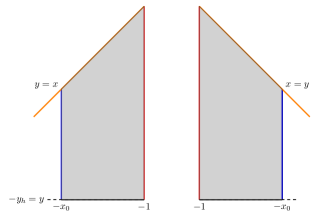
Figure 1: Two copies of the wedges.

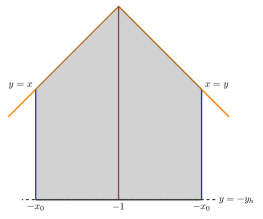
Figure 2: Gluing the EOW branes with the same color.

Figure 3: Engineer a compact black hole by gluing EOW branes.

We can introduce a new continuous angular variable as

$$x<-1,\quad x=-\cosh\psi,\quad\psi\in[-\psi_{0},\psi_{0}]\,.$$ (4)

The ”center” and event horizon of the black hole sits at $y=-\infty$ and $y=-y_{h}=-\sqrt{\frac{1+a^{2}}{a^{2}}}$. One possible way to diagnose the acceleration is to translate the C-metric into global AdS₃. We see that the ”center” of the black hole corresponds to a point situated at a distance from the AdS₃’s center, indicating that the black hole is accelerated to counteract the negative pressure of the AdS space. In four dimensions, the acceleration is sustained by cosmic strings causing conical singularities along the string due to their back-reaction on the geometry. Notably, the black hole+string system possesses a well-defined thermodynamics [23]. In contrast, EOW branes do not back-react on the geometry rendering the 4D method of thermodynamics inapplicable. In AdS/BCFT, when a Ryo-Takayanaki (RT) surface intersects with EOW branes the associated entanglement entropy will receive a contribution from the EOW branes which is referred to as the boundary entropy. In the 3D metric case, the RT surface is the black hole horizon which suggests that we should consider the black hole+EOW system.

The primary distinction between the 3D and 4D C-metrics lies in the ambiguity of the black hole’s (holographic) mass, which varies according to the chosen conformal structure . The conformal structure dictates asymptotic boundary conditions.

These novel feathers of 3D C-metric present challenges for formulating thermodynamics and holographic interpretation. Here we will address the problems in the Chern-Simons formalism of AdS gravity [51, 52] and the co-adjoint orbit theory [53]. We begin by introducing a large family of static 3D solutions that are constructed in CS formalism and then clarify some subtleties about its thermodynamics and holographic interpretation. By embedding the 3D C-metric in this family, we derive the first law of thermodynamics and a Smarr formula. In the end, we will comment on the previous results [44], where a special conformal structure was chosen.

2 Three-dimensional static solutions

Since AdS₃ pure gravity lacks a local degree of freedom, its geometric configuration only depends on the asymptotic boundary condition. Utilizing the Chern-Simons formalism, numerous static solutions have been constructed [54]. The metric for these solutions reads

$$ds^{2} = \frac{dz^{2}}{z^{2}}+\frac{1}{z^{2}}(-f^{2}dt^{2}+d\varphi^{2})+\frac{ud\varphi^{2}+f(uf-2f^{\prime\prime})dt^{2}}{2}$$ (5)

$$+z^{2}\frac{u^{2}d\varphi^{2}-(uf-2f^{\prime\prime})^{2}dt^{2}}{16},$$

where $f(\varphi),u(\varphi)$ are functions of the $\varphi$-circle $S^{1}$ and they are subject to the conditions

$$\mathcal{D}f=0,\quad\mathcal{D}\equiv(\partial_{\varphi}u)+2u\partial_{\varphi}-2\partial^{3}_{\varphi}\,,$$ (6)

which are equivalent to the Einstein’s equation. The asymptotic boundary condition is reflected in the relation between $u$ and $f$ given by

$$f=2\pi\frac{\delta\mathcal{H}}{\delta u}.$$ (7)

To support this boundary condition, the Chern-Simons action needs to be complemented by the following the surface integral

$$B_{\infty}=\frac{\kappa}{8\pi}\int dt\,\mathcal{H}.$$ (8)

The metric functions $f(\varphi)$ and $u(\varphi)$ transform under an infinitesimal diffeomorphism $\epsilon(\varphi)$ as

$$\delta f=\epsilon f^{\prime}-f\epsilon^{\prime},\quad\delta u=\mathcal{D}\epsilon.$$ (9)

The diffeomorphisms that are compatible with the boundary condition (7) define the asymptotic symmetries. In particular, the charge which is associated with the time translation invariance is $\mathcal{H}$. The transformation (9) implies that $f$ transforms like a vector in $\text{diff}(S^{1})$ and $u$ transforms like a co-vector. If $\epsilon=f$ then $\delta f=\delta u=0$ thanks to (6). By the co-adjoint orbit theory [53], the phase space of static solutions is described by the co-adjoint orbit $W_{u}=\frac{\text{diff}(S^{1})}{f}$ with centralizer $f$. In other words, if $u$ and $\tilde{u}$ belong to different orbits they cannot be interchanged by diffeomorphisms. To have a smooth geometry, we will assume that $f$ is positive definite. Thus in each orbit, We can always find a representative $\varphi_{0}\sim\varphi_{0}+2\pi$ such that $f(\varphi_{0})=f_{0}$ is constant. Other representations $\varphi$ are related to $\varphi_{0}$ via

$$\oint\frac{d\varphi_{0}}{f_{0}}=\oint\frac{d\varphi}{f(\varphi)},$$ (10)

where $L_{\varphi}$ is the circumference of the $\varphi$-circle. When $f$ is transformed into a constant, simultaneously $u$ becomes a constant due to the invariant combination

$$uf^{2}-2ff^{\prime\prime}+(f^{\prime})^{2}\equiv u_{0}f_{0}^{2},$$ (11)

under a diffeomorphism. The invariant scalar product between a vector $f$ and a co-vector $u$ can be defined as

$$\oint d\varphi\,fu-2\oint f_{0}\{\varphi,\varphi_{0}\}d\varphi_{0}=2\pi u_{0}f_{0},$$ (12)

where $\{\varphi,\varphi_{0}\}$ is the Schwarzian derivative.

To sum up, the phase space of the static solutions described by the metric (5) is the co-adjoint orbit $W_{\mu}$ which is labeled by two constant $f_{0}$ and $u_{0}$ linked by (7).

2.1 Thermodynamics and holography

The metric (5) is already written in the Fefferman-Graham (FG) gauge [55, 56] such that the holographic stress-energy tensor $T_{\mu\nu}$ [57] can be easily read off. Integrating the component $T_{tt}$ along the $S^{1}$ gives the holographic mass

$$M_{\text{holo}}[\varphi]=\frac{1}{16\pi G_{N}}\oint d\varphi fu=\frac{c}{12}u_{0}f_{0}+\frac{c}{12\pi}f_{0}\oint\{\varphi,\varphi_{0}\}d\varphi_{0},$$ (13)

where the Brown-Henneaux relation $c=3/(2G_{N})$ is used[58]. The metric (5) has an event horizon at

$$z_{h}=\sqrt{\frac{4f}{uf-2f^{\prime\prime}}},$$ (14)

which is associated with a Hawking temperature and a Bekenstein-Hawking entropy [59]:

$$T_{H}=\frac{\sqrt{u_{0}}f_{0}}{2\pi},\quad S_{BH}=\frac{\pi c}{3}\sqrt{u_{0}}\,.$$ (15)

It may be a little surprising that holographic mass $M_{\text{holo}}$ depends on the orbit representative while the black hole entropy $S_{BH}$ does not. This is due simply to the fact that the (asymptotic) charges only act on the asymptotic boundary but not on the horizon. It is also possible to define surface charges near the horizon [60] by imposing a boundary condition to the horizon instead of to the conformal boundary. They correspond to soft modes [61] which contribute to the black hole entropy but not to the mass.

Now we are ready to derive the first law by varying the solution (5). The variation can be split into two directions, along the orbit and transverse to it. The variation of $M_{\text{holo}}$ has both of these two contributions:

$$\delta M_{\text{holo}}[\varphi] = \frac{c}{12}\left(f_{0}\delta u_{0}+(u_{0}+\frac{1}{\pi}\oint\{\varphi,\varphi_{0}\})d\varphi_{0})\delta f_{0}\right)$$ (16)

$$+ \frac{c}{12\pi}f_{0}\oint\delta\left(\{\varphi,\varphi_{0}\}\right)d\varphi_{0}.$$

However, the variation of entropy is simply

$$T_{H}\delta S_{BH}=\frac{c}{12}f_{0}\delta u_{0}.$$ (17)

It suggests the first law should be modified as

$$\delta M_{\text{holo}}[\varphi]=T_{H}\delta S_{BH}+\rho_{\varphi}\delta f_{0}+\oint\Omega_{\varphi}\delta\varphi\,d\varphi_{0},$$ (18)

where we have defined

$$\rho_{\varphi} = \frac{c}{12}(u_{0}+\frac{1}{\pi}\oint d\varphi_{0}\{\varphi,\varphi_{0}\}),$$ (19)

$$\Omega_{\varphi} = \frac{c}{12\pi}\left(\frac{\varphi^{\prime\prime 2}-\varphi^{\prime\prime\prime}\varphi^{\prime}}{{\varphi^{\prime}}^{3}}\right)^{\prime}.$$ (20)

The variation $\delta f_{0}$ corresponds to the change of the proper length of the $S^{1}$ circle so $\rho_{\varphi}$ can be interpreted as the energy density. It is easy to show that $\Omega_{\varphi}=0$ when $\varphi=c_{1}+c_{2}\tanh{c_{s}(\varphi_{0}+c_{4})}\equiv\varphi_{s}$ or $\varphi=\varphi_{0}$ and in these two cases the first law reduces to the standard one

$$\delta{M}_{\text{holo}}[\varphi_{s,0}]=T_{H}\delta S_{BH}+\rho_{\varphi_{s,0}}\delta f_{0},$$ (21)

with $\rho_{\varphi_{s}}=c(u_{0}-2c_{s}^{2}/\pi)/12$ and $\rho_{0}=cu_{0}/12$.

Alternatively, we can interpret the failure of first law $\delta M_{\text{holo}}\neq T_{H}\delta S_{BH}$ as a mismatch between the holographic mass and the thermodynamics mass. Examining the asymptotic symmetry, the energy defined by asymptotic time translation invariance is $M_{\text{th}}\equiv\frac{c}{12}\mathcal{H}$ which is invariant under all the diffeomorphism compatible with the boundary conditions and thus the free energy of both the black hole and its dual boundary CFT should be [54, 59]:

$$\mathcal{F}_{\text{free}}=M_{\text{th}}-T_{H}S_{BH},$$ (22)

and the first law

$$\delta M_{\text{th}}=T_{H}\delta S_{BH},$$ (23)

directly follows from (7). The Smarr formula also takes the standard form:

$$2M_{\text{th}}=T_{H}S_{BH}.$$ (24)

The distinction between the holographic mass $M_{\text{holo}}$ and the thermodynamic mass $M_{\text{th}}$ originates from that the action of the bulk gravity theory is not simply given by standard AdS action:

$$I_{\text{AdS}}=-\frac{1}{16\pi G_{N}}\int\sqrt{g}(R+2)-\frac{1}{8\pi G_{N}}\int\sqrt{h}(K-1).$$ (25)

Indeed, substituting the Euclidean version of the metric (5) into (25) leads to the on-shell action

$$I_{\text{on-shell}}=\beta(M_{\text{holo}}-T_{H}S_{BH})\neq\mathcal{F}_{\text{free}}.$$ (26)

Motivated by new boundary term (8) in the Chern-Simon formalism, a proper boundary term should be included in (25) as well . The new boundary term can also be motived from the perspective of multi-trace deformation [63]. Only in the Brown-Henneaux boundary condition which corresponds to

$$\mathcal{H}_{BH}=\frac{1}{2\pi}\int d\varphi\,u,\quad f=1,$$ (27)

these two masses are equal: $M_{\text{th}}=M_{\text{holo}}$. In general, $\mathcal{H}(u,u^{\prime},\dots)$ can be viewed as a multi-trace deformation of $\mathcal{H}_{BH}$. For example, the simplest KdV boundary condition is described by

$$\mathcal{H}_{\text{KdV}}=\frac{1}{2\pi}\int d\varphi\,u+\frac{\lambda}{2\pi}\int d\varphi\,u^{2}\equiv Q_{1}+\lambda Q_{3}.$$ (28)

The KdV charge $Q_{3}$ of a two-dimensional conformal field theory is a double-trace operator

$$Q_{3}=\frac{1}{2\pi}\int d\varphi(TT),$$ (29)

where $T$ is the holomorphic stress-energy tensor. Following the holographic dictionary of the double-trace deformation, the deformed action should be

$$I_{Q_{1}+\lambda Q_{3}}=I_{Q_{1}}-\lambda\int dtd\varphi\frac{\delta Q_{3}}{\delta T}T.$$ (30)

Next, we apply the general analysis to the three-dimensional C-metric.

3 Application to C-metric

To compare with the standard metric (5), we first rewrite three-dimensional C-metric (1) in the FG gauge:

$$ds^{2}=\frac{1}{z^{2}}dz^{2}+\frac{1}{z^{2}}\left(g^{(0)}+z^{2}g^{(2)}+z^{4}g^{(4)}\right),$$ (31)

with

$$g^{(0)}_{ij}dx^{i}dx^{j}=-\omega(x)^{2}dt^{2}+\frac{\omega(x)^{2}dx^{2}}{(x^{2}-1)\Gamma^{2}},\quad\Gamma=1+a^{2}-a^{2}x^{2},$$ (32)

and

$$g_{tt}=\frac{1+a^{2}}{2}-\frac{(x^{2}-1)\Gamma^{2}\omega^{\prime 2}}{2\omega^{2}},$$ (33)

$$g_{xx}=\frac{1+a^{2}}{2(x^{2}-1)\Gamma^{2}}+\frac{x(1-3a^{2}(x^{2}-1))}{(x^{2}-1)\Gamma}\frac{\omega^{\prime}}{\omega}+\frac{2\omega\omega^{\prime\prime}-3\omega^{\prime 2}}{2\omega^{2}},$$ (34)

$$g^{(4)}=\frac{1}{4}g^{(2)}{g^{(0)}}^{-1}g^{(2)}.$$ (35)

Therefore, one can make the following identifications

$$f(\varphi)=\omega(x(\varphi)),\quad d\varphi=\frac{\omega dx}{\sqrt{x^{2}-1}\Gamma(x)},\quad u_{0}f_{0}^{2}=1+a^{2}.$$ (36)

We start by showing that different choice conformal factors $\omega=f$ lead to the same orbit. Let $f_{1}({\varphi_{1}})$ and $f_{2}({\varphi_{2}})$ be two choices of conformal factors. The relation (36) implies that $\varphi_{1}$ and $\varphi_{2}$ diffeomorphic to each other

$$\frac{d\varphi_{1}}{f_{1}(\varphi_{1})}=\frac{d\varphi_{2}}{f_{2}(\varphi_{2})},$$ (37)

so that $f_{1},u_{1}$ and $f_{2},u_{2}$ belong to the same co-adjoint orbit. Using the general results immediately we obtain

$$\frac{1}{f_{0}} = \frac{1}{2\pi}\int\frac{d\varphi}{f}=\frac{1}{2\pi}\int\frac{\sqrt{g^{(0)}_{xx}}dx}{\omega(x)}=\frac{L_{S^{1}}}{2\pi},$$ (38)

$$u_{0} = (1+a^{2})\left(\frac{L_{S^{1}}}{2\pi}\right)^{2},\quad T_{H}=\frac{\sqrt{1+a^{2}}}{2\pi},$$ (39)

$$\quad S_{BH} = \frac{cL_{S^{1}}}{6}\sqrt{1+a^{2}},\quad M_{\text{holo}}[\varphi]=\frac{cL_{S^{1}}}{24\pi}(1+a^{2}+\frac{1}{\pi}\oint d\varphi_{0}\{\varphi,\varphi_{0}\}),$$ (40)

where $L_{S^{1}}$ is the proper length of the (asymptotic) $S^{1}$:

$$L_{S^{1}}=\frac{2\coth^{-1}\left(\frac{x_{0}}{\sqrt{\left(a^{2}+1\right)\left(x_{0}^{2}-1\right)}}\right)}{\sqrt{a^{2}+1}}.$$ (41)

$M_{\text{th}}$ vs. $M_{\text{holo}}$. To derive $M_{\text{th}}$, in practice, one should specify the boundary condition first and then solve $f$ and $u$ according to the equations of motion (6). In the case of three-dimensional C-metric, when we choose a conformal factor $f$, the other parameter $u$ is then fixed by the identity (11) with $u_{0}f_{0}^{2}=1+a^{2}$. At once we know the functional relation between $f$ and $u$, we can use the definition of $f$ (7) to solve a suitable $M_{\text{th}}$. For example, choosing $f(\varphi_{\text{ADM}})$ to be the one appearing in the asymptotic boundary in the ADM formalism [64, 44] we find

$$f(\varphi(\varphi_{0}))=\sqrt{\frac{2(1+a^{2})}{2+a^{2}+a^{2}\cosh(2\sqrt{1+a^{2}}\varphi_{0}/f_{0})}},$$ (42)

$$u=-2-a^{2}+3f^{2},\quad\rightarrow\quad f=\sqrt{\frac{2+a^{2}+u}{3}},$$ (43)

in our convention. Integrating (7) gives the thermodynamics mass:

$$M_{\text{th}} = \frac{c}{24\pi}\int\frac{2}{3\sqrt{3}}(2+a^{2}+u)^{3/2}d\varphi$$ (44)

$$= \frac{c}{24\pi}\int 2f^{3}d\varphi\neq M_{\text{holo}}[\varphi_{\text{ADM}}].$$

ADM gauge vs. FG gauge. It is demonstrated in [44], that the 3D C-metric within the ADM gauge exhibits certain anticipated holographic characteristics. For example, the Euclidean on-shell action equates to the black hole’s free energy, and a conserved holographic stress-energy tensor can be explicitly specified. However, it is not clear how to formulate an appropriate first law of thermodynamics in ADM formalism even though that the ADM mass is consistent with our result: $M_{\text{ADM}}=M_{\text{holo}}[\varphi_{\text{ADM}}]$. Which gauge has the correct holographic description: the ADM gauge or the FG gauge? We expect that they are both correct. The difference lies in the fact that these two gauges cover different parts of the whole geometry as shown in Fig.(4). In particular, the ADM gauge covers more horizon than the FG gauge does since in the ADM gauge the black hole entropy is larger than (40) and the difference is :

$$S_{\text{ADM}}-S_{\text{FG}}=\frac{c}{3}\log\sqrt{\frac{1+a\sinh\psi_{0}}{1-a\sinh\psi_{0}}}=\frac{c}{3}\log\sqrt{\frac{1+\mu_{0}}{1-\mu_{0}}}=2g_{\mu_{0}},$$ (45)

where $\mu_{0}$ is the tension of the EOW at $x=-x_{0}(\text{or }\psi=-\psi_{0})$. The extra piece $g_{\mu_{0}}$ exactly equals the boundary entropy of the EOW brane implying that this extra entropy in the ADM gauge should be interpreted as the boundary entropy. The boundary entropy should not be included in the formulation of the first law of thermodynamics or we can add another term $-2T\delta g_{\mu_{0}}$ in the first law. Below we give a simpler example to confirm our interpretation.

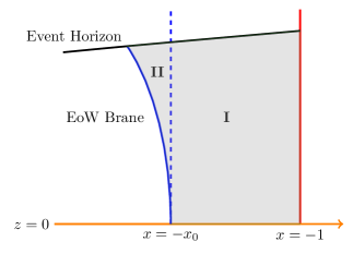
Figure 4: We have assumed that the metric (5) described two copies of the patch I. However, the EOW brane in the FG gauge is bended so the spacetime covered by the ADM gauge is I and II in the FG gauge.

A BTZ example. The metric of the (non-rotating) BTZ black hole is

$$ds^{2}=\frac{1}{z^{2}}\left({f(z)}d\tau^{2}+\frac{\operatorname{d}z^{2}}{f(z)}+dx^{2}\right),$$ (46)

where $f(z)=1-(z/z_{H})^{2},\tau\sim\tau+2\pi z_{H}$. In the BTZ geometry, the profile of the static EOW brane is [65]

$$Q_{\pm}(x_{0},\lambda):\quad z=\pm\frac{z_{H}}{\lambda}\sinh\frac{x-x_{0}}{z_{H}},\quad\lambda=|\frac{\mu}{\sqrt{1-\mu^{2}}}|,$$ (47)

which ends on the AdS boundary at $x=x_{0}$. The tensionless brane is the constant $x$ surface. Let us consider a wedge $W_{0,\lambda}$ bounded by $x=0$ and a EOW brane $Q_{+}(x_{0},\lambda)$ and a wedge $W_{0,0}$ bounded by $x=0$ and $x=x_{0}$. In the wedge $W_{0,0}$, the holographic mass, temperature and the entropy are

$$T=\frac{1}{2\pi z_{H}},\quad S=\frac{cx_{0}}{6z_{H}},\quad M=\frac{cx_{0}}{24\pi z_{H}^{2}},$$ (48)

which satisfies the first law

$$dM=-\frac{cx_{0}}{12\pi z_{H}^{3}}dz_{H}=TdS.$$ (49)

However, for the wedge $W_{0,\lambda}$ we have

$$T=\frac{1}{2\pi z_{H}},\quad S_{\lambda}=\frac{cx_{0}}{6z_{H}}+\frac{c}{6}\sinh^{-1}\lambda,\quad M=\frac{cx_{0}}{24\pi z_{H}^{2}}.$$ (50)

The difference of $S_{\lambda}$ and $S$ is exactly the boundary entropy corresponding to the horizon area difference in these two wedges.

4 Conclusions and Outlook

In this work, we have described the thermodynamics and holographic properties of three-dimensional accelerating black holes in a more general and systematic way. In contrast to the previous discussion in the ADM formalism [44], our description is universal for all the choices of the conformal structure and with the help of the Chern-Simons formalism of the AdS gravity, the connection between the asymptotic boundary condition and the free energy can be built so that a proper first law of thermodynamics and the Smarr formula can be derived. The correct free energy is the starting point to study its phase transition, for example, the Hawking-Page phase transition [66]. The KdV black holes have a very fruitful phase structure [59, 67], and we expect a similar phenomenon will happen in three-dimensional accelerating black holes.

The static solution (5) can be generalized to include angular momentum very easily by exciting non-equal left $u,f$ and right $\bar{u},\bar{f}$ movers. Then it is very promising to construct an accelerating black hole with rotation in the FG gauge. The free energy will be simply given by $\mathcal{F}+\bar{\mathcal{F}}$. The challenge is to rewrite the solution in the “intrinsic” gauge like (1) because the coordinate transformation between (1) and the FG gauge is only known as an infinite series expansion of $z$. It is also interesting to generalize our approach to describe the charged accelerating BTZ black holes [5].

On the holographic property, it is important to study the entanglement entropy. As we have shown the bulk theory is not just the AdS Einstein gravity in general. It is possible that RT formula $S_{A}=\frac{\text{Area}_{A}}{4G_{N}}$ is modified. Moreover, the EOW branes also serve as RT surface anchors which may lead to a phase transition of entanglement entropy. We leave these interesting questions in the future work.

Finally, it is worth revisiting Class I and Class III type solutions in our approach. In particular, the Class I_C solution describes an accelerating black hole solution parametrically disconnected from the standard BTZ geometry. The difference between the Class I_C solution and the Class II solution may be more transparent in our approach.

References

- [1] Juan Martin Maldacena “The Large N limit of superconformal field theories and supergravity” In Adv. Theor. Math. Phys. 2, 1998, pp. 231–252 DOI: 10.4310/ATMP.1998.v2.n2.a1
- [2] Edward Witten “Anti-de Sitter space and holography” In Adv. Theor. Math. Phys. 2, 1998, pp. 253–291 DOI: 10.4310/ATMP.1998.v2.n2.a2
- [3] S.. Gubser, Igor R. Klebanov and Alexander M. Polyakov “Gauge theory correlators from noncritical string theory” In Phys. Lett. B 428, 1998, pp. 105–114 DOI: 10.1016/S0370-2693(98)00377-3
- [4] Gabriel Arenas-Henriquez, Ruth Gregory and Andrew Scoins “On acceleration in three dimensions” In JHEP 05, 2022, pp. 063 DOI: 10.1007/JHEP05(2022)063
- [5] B. Eslam Panah “Charged Accelerating BTZ Black Holes” In Fortsch. Phys. 71.8-9, 2023, pp. 2300012 DOI: 10.1002/prop.202300012
- [6] Patricio S. Letelier and Samuel R. Oliveira “On uniformly accelerated black holes” In Phys. Rev. D 64, 2001, pp. 064005 DOI: 10.1103/PhysRevD.64.064005
- [7] J. Bicak and Vojtech Pravda “Spinning C metric: Radiative space-time with accelerating, rotating black holes” In Phys. Rev. D 60, 1999, pp. 044004 DOI: 10.1103/PhysRevD.60.044004
- [8] Jiri Podolsky and J.. Griffiths “Null limits of the C metric” In Gen. Rel. Grav. 33, 2001, pp. 59–64 DOI: 10.1023/A:1002023918883
- [9] Vojtech Pravda and A. Pravdova “Coaccelerated particles in the C metric” In Class. Quant. Grav. 18, 2001, pp. 1205–1216 DOI: 10.1088/0264-9381/18/7/305
- [10] Oscar J.. Dias and Jose P.. Lemos “Pair of accelerated black holes in anti-de Sitter background: AdS C metric” In Phys. Rev. D 67, 2003, pp. 064001 DOI: 10.1103/PhysRevD.67.064001
- [11] J.. Griffiths and J. Podolsky “A New look at the Plebanski-Demianski family of solutions” In Int. J. Mod. Phys. D 15, 2006, pp. 335–370 DOI: 10.1142/S0218271806007742
- [12] Pavel Krtous “Accelerated black holes in an anti-de Sitter universe” In Phys. Rev. D 72, 2005, pp. 124019 DOI: 10.1103/PhysRevD.72.124019
- [13] Fay Dowker, Jerome P. Gauntlett, David A. Kastor and Jennie H. Traschen “Pair creation of dilaton black holes” In Phys. Rev. D 49, 1994, pp. 2909–2917 DOI: 10.1103/PhysRevD.49.2909
- [14] Roberto Emparan, Gary T. Horowitz and Robert C. Myers “Exact description of black holes on branes” In JHEP 01, 2000, pp. 007 DOI: 10.1088/1126-6708/2000/01/007
- [15] Roberto Emparan, Gary T. Horowitz and Robert C. Myers “Exact description of black holes on branes. 2. Comparison with BTZ black holes and black strings” In JHEP 01, 2000, pp. 021 DOI: 10.1088/1126-6708/2000/01/021
- [16] Roberto Emparan, Ruth Gregory and Caroline Santos “Black holes on thick branes” In Phys. Rev. D 63, 2001, pp. 104022 DOI: 10.1103/PhysRevD.63.104022
- [17] Ruth Gregory, Simon F. Ross and Robin Zegers “Classical and quantum gravity of brane black holes” In JHEP 09, 2008, pp. 029 DOI: 10.1088/1126-6708/2008/09/029
- [18] Roberto Emparan, Antonia Micol Frassino and Benson Way “Quantum BTZ black hole” In JHEP 11, 2020, pp. 137 DOI: 10.1007/JHEP11(2020)137
- [19] H. Lü and Justin F. Vázquez-Poritz “C-metrics in Gauged STU Supergravity and Beyond” In JHEP 12, 2014, pp. 057 DOI: 10.1007/JHEP12(2014)057
- [20] Pietro Ferrero et al. “Accelerating black holes and spinning spindles” In Phys. Rev. D 104.4, 2021, pp. 046007 DOI: 10.1103/PhysRevD.104.046007
- [21] Davide Cassani, Jerome P. Gauntlett, Dario Martelli and James Sparks “Thermodynamics of accelerating and supersymmetric AdS4 black holes” In Phys. Rev. D 104.8, 2021, pp. 086005 DOI: 10.1103/PhysRevD.104.086005
- [22] Pietro Ferrero, Matteo Inglese, Dario Martelli and James Sparks “Multicharge accelerating black holes and spinning spindles” In Phys. Rev. D 105.12, 2022, pp. 126001 DOI: 10.1103/PhysRevD.105.126001
- [23] Michael Appels, Ruth Gregory and David Kubiznak “Thermodynamics of Accelerating Black Holes” In Phys. Rev. Lett. 117.13, 2016, pp. 131303 DOI: 10.1103/PhysRevLett.117.131303
- [24] Marco Astorino “CFT Duals for Accelerating Black Holes” In Phys. Lett. B 760, 2016, pp. 393–405 DOI: 10.1016/j.physletb.2016.07.019
- [25] Michael Appels, Ruth Gregory and David Kubiznak “Black Hole Thermodynamics with Conical Defects” In JHEP 05, 2017, pp. 116 DOI: 10.1007/JHEP05(2017)116
- [26] Andrés Anabalón et al. “Holographic Thermodynamics of Accelerating Black Holes” In Phys. Rev. D 98.10, 2018, pp. 104038 DOI: 10.1103/PhysRevD.98.104038
- [27] Andrés Anabalón et al. “Thermodynamics of Charged, Rotating, and Accelerating Black Holes” In JHEP 04, 2019, pp. 096 DOI: 10.1007/JHEP04(2019)096
- [28] Behzad Eslam Panah and Khadijie Jafarzade “Thermal stability, criticality and heat engine of charged rotating accelerating black holes” In Gen. Rel. Grav. 54.2, 2022, pp. 19 DOI: 10.1007/s10714-022-02904-9
- [29] Ruth Gregory and Andrew Scoins “Accelerating Black Hole Chemistry” In Phys. Lett. B 796, 2019, pp. 191–195 DOI: 10.1016/j.physletb.2019.06.071
- [30] Adam Ball and Noah Miller “Accelerating black hole thermodynamics with boost time” In Class. Quant. Grav. 38.14, 2021, pp. 145031 DOI: 10.1088/1361-6382/ac0766
- [31] Adam Ball “Global first laws of accelerating black holes” In Class. Quant. Grav. 38.19, 2021, pp. 195024 DOI: 10.1088/1361-6382/ac2139
- [32] Ruth Gregory, Zheng Liang Lim and Andrew Scoins “Thermodynamics of Many Black Holes” In Front. in Phys. 9, 2021, pp. 187 DOI: 10.3389/fphy.2021.666041
- [33] Hyojoong Kim, Nakwoo Kim, Yein Lee and Aaron Poole “Thermodynamics of accelerating AdS4 black holes from the covariant phase space”, 2023 arXiv:2306.16187 [hep-th]
- [34] Gérard Clément and Dmitry Gal’tsov “The first law for stationary axisymmetric multi-black hole systems” In Phys. Lett. B 845, 2023, pp. 138152 DOI: 10.1016/j.physletb.2023.138152
- [35] Veronika E. Hubeny, Donald Marolf and Mukund Rangamani “Black funnels and droplets from the AdS C-metrics” In Class. Quant. Grav. 27, 2010, pp. 025001 DOI: 10.1088/0264-9381/27/2/025001
- [36] Pietro Ferrero et al. “D3-Branes Wrapped on a Spindle” In Phys. Rev. Lett. 126.11, 2021, pp. 111601 DOI: 10.1103/PhysRevLett.126.111601
- [37] Pietro Ferrero, Jerome P. Gauntlett and James Sparks “Supersymmetric spindles” In JHEP 01, 2022, pp. 102 DOI: 10.1007/JHEP01(2022)102
- [38] Andrea Boido, Jerome P. Gauntlett, Dario Martelli and James Sparks “Entropy Functions For Accelerating Black Holes” In Phys. Rev. Lett. 130.9, 2023, pp. 091603 DOI: 10.1103/PhysRevLett.130.091603
- [39] J.. Griffiths, P. Krtous and J. Podolsky “Interpreting the C-metric” In Class. Quant. Grav. 23, 2006, pp. 6745–6766 DOI: 10.1088/0264-9381/23/23/008
- [40] Kh. Jafarzade, J. Sadeghi, B. Panah and S.. Hendi “Geometrical thermodynamics and P-V criticality of charged accelerating AdS black holes” In Annals Phys. 432, 2021, pp. 168577 DOI: 10.1016/j.aop.2021.168577
- [41] Filip Landgren and Arvind Shekar “Islands and entanglement entropy in -dimensional curved backgrounds”, 2024 arXiv:2401.01653 [hep-th]
- [42] Marco Astorino “Accelerating black hole in 2+1 dimensions and 3+1 black (st)ring” In JHEP 01, 2011, pp. 114 DOI: 10.1007/JHEP01(2011)114
- [43] Wei Xu, Kun Meng and Liu Zhao “Accelerating BTZ spacetime” In Class. Quant. Grav. 29, 2012, pp. 155005 DOI: 10.1088/0264-9381/29/15/155005
- [44] Gabriel Arenas-Henriquez, Adolfo Cisterna, Felipe Diaz and Ruth Gregory “Accelerating black holes in 2 + 1 dimensions: holography revisited” In JHEP 09, 2023, pp. 122 DOI: 10.1007/JHEP09(2023)122
- [45] B. Eslam Panah “Three-dimensional energy-dependent C-metric: Black hole solutions” In Phys. Lett. B 844, 2023, pp. 138111 DOI: 10.1016/j.physletb.2023.138111
- [46] B. Eslam Panah, M. Khorasani and J. Sedaghat “Three-dimensional accelerating AdS black holes in F(R) gravity” In Eur. Phys. J. Plus 138.8, 2023, pp. 728 DOI: 10.1140/epjp/s13360-023-04339-w
- [47] Adolfo Cisterna, Felipe Diaz, Robert B. Mann and Julio Oliva “Exploring accelerating hairy black holes in 2+1 dimensions: the asymptotically locally anti-de Sitter class and its holography” In JHEP 11, 2023, pp. 073 DOI: 10.1007/JHEP11(2023)073
- [48] Tadashi Takayanagi “Holographic Dual of BCFT” In Phys. Rev. Lett. 107, 2011, pp. 101602 DOI: 10.1103/PhysRevLett.107.101602
- [49] Mitsutoshi Fujita, Tadashi Takayanagi and Erik Tonni “Aspects of AdS/BCFT” In JHEP 11, 2011, pp. 043 DOI: 10.1007/JHEP11(2011)043
- [50] Ioannis Papadimitriou and Kostas Skenderis “Thermodynamics of asymptotically locally AdS spacetimes” In JHEP 08, 2005, pp. 004 DOI: 10.1088/1126-6708/2005/08/004
- [51] A. Achucarro and P.. Townsend “A Chern-Simons Action for Three-Dimensional anti-De Sitter Supergravity Theories” In Phys. Lett. B 180, 1986, pp. 89 DOI: 10.1016/0370-2693(86)90140-1
- [52] Edward Witten “(2+1)-Dimensional Gravity as an Exactly Soluble System” In Nucl. Phys. B 311, 1988, pp. 46 DOI: 10.1016/0550-3213(88)90143-5
- [53] Edward Witten “Coadjoint Orbits of the Virasoro Group” In Commun. Math. Phys. 114, 1988, pp. 1 DOI: 10.1007/BF01218287
- [54] Alfredo Pérez, David Tempo and Ricardo Troncoso “Boundary conditions for General Relativity on AdS3 and the KdV hierarchy” In JHEP 06, 2016, pp. 103 DOI: 10.1007/JHEP06(2016)103
- [55] C Robin Graham “Charles Fefferman” In Astérisque 131, 1985, pp. 95–116
- [56] Charles Fefferman and C. Graham “The ambient metric” In Ann. Math. Stud. 178, 2011, pp. 1–128 arXiv:0710.0919 [math.DG]
- [57] Vijay Balasubramanian and Per Kraus “A Stress tensor for Anti-de Sitter gravity” In Commun. Math. Phys. 208, 1999, pp. 413–428 DOI: 10.1007/s002200050764
- [58] J. Brown and M. Henneaux “Central Charges in the Canonical Realization of Asymptotic Symmetries: An Example from Three-Dimensional Gravity” In Commun. Math. Phys. 104, 1986, pp. 207–226 DOI: 10.1007/BF01211590
- [59] Anatoly Dymarsky and Sotaro Sugishita “KdV-charged black holes” In JHEP 05, 2020, pp. 041 DOI: 10.1007/JHEP05(2020)041
- [60] Daniel Grumiller et al. “Spacetime structure near generic horizons and soft hair” In Phys. Rev. Lett. 124.4, 2020, pp. 041601 DOI: 10.1103/PhysRevLett.124.041601
- [61] Stephen W. Hawking, Malcolm J. Perry and Andrew Strominger “Soft Hair on Black Holes” In Phys. Rev. Lett. 116.23, 2016, pp. 231301 DOI: 10.1103/PhysRevLett.116.231301
- [62] Cristián Erices, Miguel Riquelme and Pablo Rodríguez “BTZ black hole with Korteweg–de Vries-type boundary conditions: Thermodynamics revisited” In Phys. Rev. D 100.12, 2019, pp. 126026 DOI: 10.1103/PhysRevD.100.126026
- [63] Edward Witten “Multitrace operators, boundary conditions, and AdS / CFT correspondence”, 2001 arXiv:hep-th/0112258
- [64] Richard Arnowitt, Stanley Deser and Charles W Misner “Coordinate invariance and energy expressions in general relativity” In Physical Review 122.3 APS, 1961, pp. 997
- [65] Mitsutoshi Fujita, Tadashi Takayanagi and Erik Tonni “Aspects of AdS/BCFT” In JHEP 11, 2011, pp. 043 DOI: 10.1007/JHEP11(2011)043
- [66] S.. Hawking and Don N. Page “Thermodynamics of Black Holes in anti-De Sitter Space” In Commun. Math. Phys. 87, 1983, pp. 577 DOI: 10.1007/BF01208266
- [67] Liangyu Chen, Anatoly Dymarsky, Jia Tian and Huajia Wang “Holographic renyi entropy in 2d CFT ensembles with fixed KdV charges”, To appear