Energy Efficiency Maximization for Intelligent Surfaces Aided Massive MIMO with Zero Forcing

Abstract

In this work, we address the energy efficiency (EE) maximization problem in a downlink communication system utilizing reconfigurable intelligent surface (RIS) in a multi-user massive multiple-input multiple-output (mMIMO) setup with zero-forcing (ZF) precoding. The channel between the base station (BS) and RIS operates under a Rician fading with Rician factor $K_{1}$. Since systematically optimizing the RIS phase shifts in each channel coherence time interval is challenging and burdensome, we employ the statistical channel state information (CSI)-based optimization strategy to alleviate this overhead. By treating the RIS phase shifts matrix as a constant over multiple channel coherence time intervals, we can reduce the computational complexity while maintaining an interesting performance. Based on an ergodic rate (ER) lower bound closed-form, the EE optimization problem is formulated. Such a problem is non-convex and challenging to tackle due to the coupled variables. To circumvent such an obstacle, we explore the sequential optimization approach where the power allocation vector $\mathbf{p}$, the number of antennas $M$, and the RIS phase shifts $\mathbf{v}$ are separated and sequentially solved iteratively until convergence. With the help of the Lagrangian dual method, fractional programming (FP) techniques, and supported by Lemma 1, insightful compact closed-form expressions for each of the three optimization variables are derived. Simulation results validate the effectiveness of the proposed method across different generalized channel scenarios, including non-line-of-sight (NLoS) ($K_{1}=0$) and partially line-of-sight (LoS) ($K_{1}\neq 0$) conditions. Our numerical results demonstrate an impressive performance of the proposed Statistical CSI-based EE optimization method, achieving $\approx 92\%$ of the performance attained through perfect instantaneous CSI-based EE optimization. This underscores its potential to significantly reduce power consumption, decrease the number of active antennas at the base station, and effectively incorporate RIS structure in mMIMO communication setup with just statistical CSI knowledge.

I Introduction

Reconfigurable intelligent surfaces is one of the most promising recent techniques that have the potential to integrate future communications systems (beyond fifth generation, 6G, etc.) due to its potential to improve the transmission by creating a “virtual” reconfigurable communication link. Specifically, the RIS is composed of several individually scattering elements which are artificial meta-material structures that can reflect incident electromagnetic waves and can be configured to increase the signal level in a specific direction[1, 2].

On the other hand, to enhance the spectral efficiency (SE) and to serve a plurality of user’s equipment (UE) using the same physical layer resources, mMIMO is essential; however, this technology resorts to hundreds of antennas operating at the BS [3], which can significantly increase the consumption.

RIS and mMIMO technologies hold great promise for the future of communication systems. As these technologies are set to play a vital role in the next-generation wireless networks, which will need to support exceptionally high data rates and accommodate a vast number of connected UE s [4, 5], there is a growing concern about their impact on energy consumption. Hence, it is imperative to focus on EE, measured in bits-per-joule, as a pivotal performance metric to ensure the development of environmentally friendly and sustainable communication systems.

An extensive number of works such as in [6, 7, 8, 9, 10, 11, 12, 13, 14, 15, 16, 17, 18, 19, 20, 21, 22] have studied the RIS deployment impact in mMIMO systems under different objectives, such as RIS-assisted sensing [6, 7, 8], minimizing the total transmit power [9], maximizing the weighted sum-rate (WSR) [10], maximizing the minimum rate [11, 12, 13], and maximizing the EE [14, 15, 16, 17, 18]. All of the above-cited studies clearly demonstrate the immense potential and versatility of RIS within wireless systems.

It is worth noting that all the previously mentioned studies assume the transmitter to access the instantaneous CSI. However, in practical applications, obtaining precise instantaneous CSI in RIS-enhanced mMIMO systems can be quite challenging. This challenge becomes even more pronounced in scenarios with high mobility and short channel coherence times. To address this issue, in [19], the authors derived a rigorous tight closed-form expression for the ER of a multi-user RIS-aided mMIMO system employing ZF precoding over Rician fading. This analysis takes into account the optimization of RIS phase shifts based on derived statistical closed-form expression, offering a more practical and robust approach in scenarios where instantaneous CSI may not be readily available or reliable. In [20], the authors exploit the long-term statistical CSI to optimize the RIS phase shifts aiming to maximize the achievable rate with maximum ratio combining (MRC), where a genetic algorithm is deployed. In [21], the authors leverage the statistical CSI optimization in order to optimize the beamforming at BS, passive beamforming at RIS, and the power of the UE s, while considering maximum UE s’s exposure to electromagnetic fields. In [22], the authors investigated the EE optimization in a RIS-assisted mMIMO scenario with one single user based on statistical-CSI optimization. The authors show the potential of optimizing the RIS phase shifts, BS transmit beamforming, and the UE s’s power.

To emphasize and highlight the significance and advantages of the statistical CSI-based optimization approach, Figure 1 demonstrates the substantial time overhead associated with adopting instantaneous CSI-based optimization compared to statistical CSI-based optimization methods. With the statistical CSI-based optimization, there is no need to continuously optimize the RIS phase shifts during various subsequent channel coherence times. This reduction in overhead leads to enhanced payload data efficiency, making it a practical choice for challenging scenarios in RIS-assisted mMIMO systems. Hence, the long-term statistical CSI-based optimization strategy could be more practical and feasible [20].

Furthermore, joint beamforming and phase shift optimization are extremely significant in order to improve the performance of wireless communication systems, particularly in RIS-aided mMIMO systems. On the other hand, several works in recent literature deploy a ZF-based precoding scheme instead of directly optimizing the precoding policy. Herein, we adopt ZF linear precoding motivated by two facts. First, we have opted for the well-established linear precoder ZF to circumvent the challenges posed by optimal precoding design in RIS-aided mMIMO design. Second, our work is primarily motivated by the concept of statistical CSI optimization, which has the potential to significantly alleviate the overhead associated with the RIS phase shifts optimization procedure within each channel coherence time. We are interested in revealing the improvements attainable through instantaneous CSI optimization and emphasize the relevance of the statistical CSI optimization approach in RIS-aided mMIMO design since such an approach can substantially reduce system complexity with only a marginal performance degradation.

Novelty: To the best of our knowledge, the EE optimization problem with statistical CSI under Rician fading for multi-user RIS-aided mMIMO systems with ZF has not yet been thoroughly investigated. This knowledge gap has motivated us to embark on resolving this important challenge. In our work, unlike previous works, such as [14, 15, 17, 18], the EE optimization problem is approached in a multi-user RIS-aided mMIMO with statistical CSI where an alternating optimization strategy is proposed to find the number of BS antennas ($M$), the RIS phase shifts ($\bf v$), and the transmit power allocation ($\bf p$) to maximize the EE. Moreover, our approach distinguishes itself from that presented in [21] by not only considering statistical CSI but also incorporating ZF precoding and the optimization of active antennas at the BS. Similarly, in [22], although the consideration of statistical CSI is similar, the crucial multi-user scenario was overlooked. Our research goes a step further by providing novel closed-form solutions for all optimization variables, thereby expanding the scope of active antennas and power allocation beyond the established boundaries of the traditional mMIMO scenario for the domain of RIS-assisted configurations. Lastly, but equally important, in contrast to the conventional EE solutions found in existing literature, which often rely on a couple of optimization techniques, namely semidefinite relaxation (SDR), sequential fractional programming (SFP), or Manifold optimization, our study, supported by Lemma 1, introduces a novel and straightforward closed-form solution for the quadratic programming problem involving the non-convex unit modulus constraint.

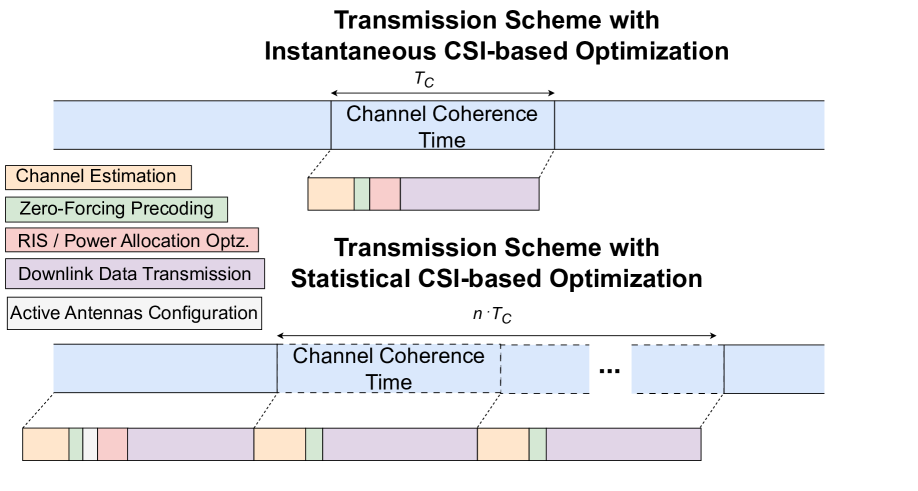
Figure 1: Illustration of the advantages by adopting Statistical CSI-based parameters optimization, where the RIS phase shifts vector ($\bf v$), transmit power allocation ($\bf p$), and the number of BS antennas ($M$) remain fixed for the UE s over multiple channel coherence times ($nT_{c}$); differently, for the Instantaneous CSI-based parameter optimization approach, where the channel estimation, precoding, RIS phase shifts, and transmit power must be updated at each $T_{c}$.

The main contributions of this work are fourfold:

• In this study, we have formulated a comprehensive non-convex optimization problem encompassing multiple key variables in a multi-user RIS-aided mMIMO system, such as the UE s’s transmit power, the quantity of active base station antennas, and the phase shifts associated with the RIS elements. We also have addressed the constraints linked to the overall power budget, the assurance of quality of service (QoS), and the necessity for unit module values since we consider only passive RIS. In addition, we have embraced the utilization of linear ZF precoding, wherein the feasibility of ZF is a pivotal consideration. Our approach extends further by proposing an innovative solution that culminates in simple yet accurately derived closed-form expressions for all the variables at hand. Specifically, for the phase shifts on the RIS optimization, the closed-form solution is an interesting alternative for the SDR, SFP, and Manifold optimization.

• Different from the previous works [14, 15, 16, 17, 18, 21, 22], the formulated EEs maximization problem relies upon only the statistical CSI estimates, which can be beneficial in short channel coherence time wireless scenarios; indeed, such an approach does not need precise instantaneous CSI estimates given optimizing the RIS phase shifts and power allocation, reducing the overhead imposed by the optimization procedure of these variables in every channel coherence time and easing the practical implementation of the RIS-assisted system.

• To deal with this problem, we apply the Lagrangian dual method with FP techniques to solve the non-convex problem. Specifically for the RIS phase shifts problem, we proposed an innovative FP-based RIS phase shifts optimization, which enables us to find a closed-form expression for each element of RIS. To support our findings, the complexity of the proposed antenna, power allocation, and RIS phase shifts optimization algorithm has been accurately investigated.

• Extensive numerical results corroborate the effectiveness and efficiency of the proposed analytical EE optimization method for RIS-aided mMIMO systems with ZF operating under generalized Rician channels. The proposed method has exhibited superior system performance in comparison to the gradient descent method. Moreover, its potential has been highlighted through promising results in contrast to the optimization based on instantaneous CSI-based optimization strategy.

The remainder of this paper is organized as follows. Section II describes the RIS-aided mMIMO system model. The optimization problem and the overall proposed analytical optimization methods and algorithms are developed and discussed in Section III. We present numerical results corroborating our findings in Section IV. Final remarks are offered in Section V.

Notations: Scalars, vectors, and matrices are denoted by the lower-case, bold-face lower-case, and bold-face upper-case letters, respectively; $\mathbb{C}^{A\times B}$ denotes the space of $A$ rows and $B$ columns complex matrices; $|\cdot|$ denote the absolute operator; ${\rm diag}(\cdot)$ denotes the diagonal operator; ${\rm Tr}(\cdot)$ is trace operator; $\left[x\right]^{+}$ denotes $\max(x,0)$; $[x]^{a}_{b}$ denotes $\min(\max(x,b),a)$; $[\cdot]^{*}$ denote the conjugate operator; $\angle[\cdot]$ denotes the phase of the complex argument; $j\triangleq\sqrt{-1}$; $\mathbb{E}\left[\cdot\right]$ is the expectation operator; $[\cdot]^{T}$ is the transpose operator; $[\cdot]^{H}$ is the conjugate transpose (Hermitian) operator; $\mathbf{I}_{K}$ stands for the $K\times K$ identity matrix; $\mathbf{X}^{-1}$ is the inverse of $X$; ${\rm det}(\cdot)$ is the determinant of a given matrix; ${\rm Re}(\cdot)$ is the real part of a complex value; $\mathcal{CN}(\mu,\sigma^{2})$ defines a complex-valued Gaussian random variable with mean $\mu$ and variance $\sigma^{2}$; $x\sim\mathcal{U}[a,b]$ defines a uniform random variable from range of $a$ to $b$; $\left\lceil\cdot\right\rceil$ denotes the ceiling function; $[\mathbf{X}]_{k,l}$ stands for the entry at $k$-th row and $l$-th column of matrix $\mathbf{X}$; $[\mathbf{X}]_{k,:}$ denotes the $k$-th row vector of matrix $\mathbf{X}$; $[\mathbf{X}]_{:,k}$ denotes the $k$-th column vector of matrix $\mathbf{X}$; $[\mathbf{X}]_{a:b,c:d}$ represents the sub-matrix of $\mathbf{X}$ consisting of rows from $a$ to $b$ and columns from $c$ to $d$; The notation $\mathcal{O}(\cdot)$ denotes the computational complexity.

II System Model

We consider a single-cell multi-user RIS-aided mMIMO system operating in downlink mode, where the BS is equipped with a uniform linear array (ULA) with $M_{\max}$ antennas, where $M$ antennas will be activated to serve $K$ single-antenna UE s. In this work, we have considered the context of far-field communication, which entails that each antenna has an equitable contribution to the system’s overall performance. The single RIS panel is equipped with $N$ elements and deployed to improve the network communication’s reliability and coverage. Fig. 2 illustrates the general RIS mMIMO system and channel scenarios investigated.

Let us denote $\mathbf{D}\in\mathbb{C}^{M\times K}$ as the direct link communication channel between the UE s and the BS, given by

$$\mathbf{D}=\tilde{\mathbf{D}}\boldsymbol{\alpha}_{D}^{1/2},$$ (1)

where $\boldsymbol{\alpha}_{D}={\rm diag}(\left[\alpha_{D,1},\dots,\alpha_{D,K}\right])$ and $\alpha_{D,k}$ denotes the large-scale fading term between the BS and the $k$-th UE, the matrix $\tilde{\mathbf{D}}\in\mathbb{C}^{M\times K}$ is composed by independent and identically distributed (i.i.d) complex Gaussian random variables, whose mean is zero and variance is unit, $i.e.$ $d_{m,k}\sim\mathcal{CN}(0,1)$, $\forall k=1,\dots,K$ and $m=1,\dots,M$.

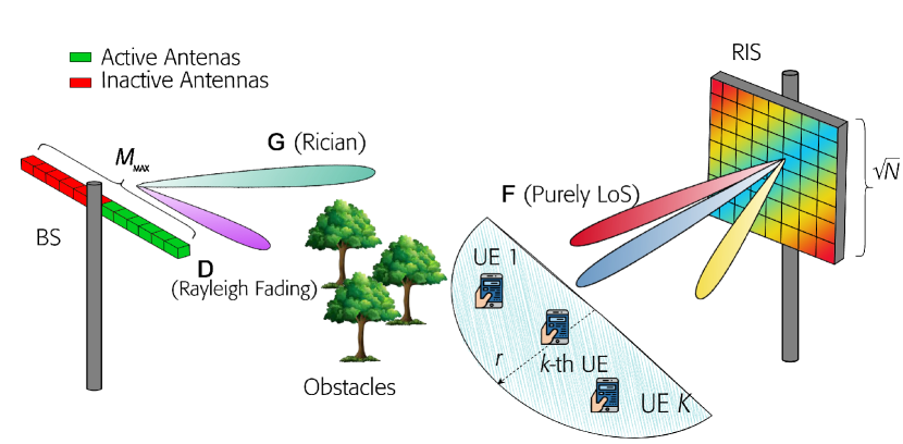
Figure 2: RIS-aided mMIMO multi-user investigated scenarios. Particularly, this setup is illustrated with $N=64$ reflective elements at RIS and $M_{\max}=12$ BS antennas; in this specific configuration, there are $M=6$ actives elements at BS.

We define the channel between the RIS and the BS as $\mathbf{G}\in\mathbb{C}^{M\times N}$ and the channel between the UE s and the RIS as $\mathbf{F}\in\mathbb{C}^{N\times K}$. The channel matrix $\mathbf{G}$ is assumed to be a Rician fading channel and can be given as [19]

$$\mathbf{G}=\sqrt{\alpha_{G}\dfrac{1}{K_{1}+1}}\mathbf{G}_{\rm{NLoS}}+\sqrt{\alpha_{G}\dfrac{K_{1}}{K_{1}+1}}\mathbf{G}_{\rm{LoS}},$$ (2)

where $\alpha_{G}$ is the large-scale fading (path loss) between the RIS and the BS and $K_{1}$ denotes the Rician factor. Besides, the fading channel matrix $\mathbf{F}$ is assumed to be purely LoS and expressed as

$$\mathbf{F}=\mathbf{F}_{\rm{LoS}}\boldsymbol{\alpha}_{F}^{1/2}=[\sqrt{\alpha_{F,1}}\mathbf{f}^{1}_{\rm{LoS}},\dots,\sqrt{\alpha_{F,K}}\mathbf{f}^{K}_{\rm{LoS}}],$$ (3)

where $\boldsymbol{\alpha}_{F}={\rm diag}([\alpha_{F,1},\dots,\alpha_{F,K}])$ and $\alpha_{F,k}$ denotes the large-scale fading factor between the $k$-th UE and the BS. Besides, the LoS channel for RIS adopted herein is based on the two-dimensional uniform squared planar array (USPA) and given as [23]

$$\mathbf{a}_{N}(\varphi,\phi) = \left[1,\dots,e^{j2\pi\frac{d}{\lambda}(x\sin\phi\sin\varphi+y\cos\phi)},\right.$$ (4)

$$\dots ,\left.e^{j2\pi\frac{d}{\lambda}\left(\left(X-1\right)\sin\phi\sin\varphi+\left(Y-1\right)\cos\phi\right)}\right]^{T},$$

where $0\leq x,y<X$ with $X=Y\in{\mathbb{Z}_{+}}$ being the square side of the USPA [24], [25], $d$ denotes the element spacing, $\lambda$ denotes the wavelength, $\varphi$ and $\phi$ are azimuth and elevation angles respectively. Let us denote $\varphi_{\rm{AoD}}^{bs}$ the angle of departure (AoD) from the BS towards the RIS, $\varphi_{{\rm AoD}}^{r,k}$ and $\phi_{\rm{AoD}}^{r,k}$ the AoD from RIS towards the $k$-th UE and $\varphi_{{\rm AoA}}^{r}$ and $\phi_{{\rm AoA}}^{r}$ the angle of arrival (AoA) at the RIS from the BS respectively. Moreover, the LoS channel for BS is based on the ULA, given by [26]

$$\mathbf{a}_{M}(\varphi) = \left[1,\dots,e^{j2\pi\frac{d}{\lambda}x\sin\varphi},e^{j2\pi\frac{d}{\lambda}\left(\left(X-1\right)\sin\varphi\right)}\right]^{T}.$$ (5)

Under this condition, the LoS channel matrix $\mathbf{G}_{{\rm LoS}}$ is expressed as

$$\mathbf{G}_{{\rm LoS}}=\mathbf{a}_{M}(\varphi_{{\rm AoD}}^{bs})\mathbf{a}_{N}(\varphi_{{\rm AoA}}^{r},\phi_{{\rm AoA}}^{r})\triangleq\mathbf{a}_{M}\mathbf{a}_{N}^{H},$$ (6)

and the LoS component $\mathbf{f}_{{\rm LoS}}^{k}$ is

$$\mathbf{f}_{{\rm LoS}}^{k}=\mathbf{a}_{N}(\varphi_{{\rm AoD}}^{r,k},\phi_{{\rm AoD}}^{r,k}).$$ (7)

The phase shifts matrix of the RIS can be defined as

$$\mathbf{\Phi}=\text{diag}(\mathbf{v}),\quad\mathbf{v}=[e^{-j\theta_{1}},\dots,e^{-j\theta_{N}}]^{H}$$ (8)

and $\theta_{n}$ is the phase shift of the $n$-th RIS element. In this way, the cascaded channel can be written as $\mathbf{H}=\mathbf{D}+\mathbf{G}\mathbf{\Phi}\mathbf{F}$.

The received signal $y_{k}$ at the $k$-th UE is

$$y_{k}=\sqrt{p_{k}}\mathbf{h}^{H}_{k}\mathbf{w}_{k}s_{k}+\sum_{j=1,j\neq k}^{K}\sqrt{p_{j}}\mathbf{h}_{k}^{H}\mathbf{w}_{j}s_{j}+n_{k},$$ (9)

where $\mathbf{h}_{k}$ and $\mathbf{w}_{k}$ is the $k$-th column of $\mathbf{H}$ and $\mathbf{W}$ respectively with $\mathbf{W}$ being the precoding matrix, $n_{k}$ is the i.i.d. additive white Gaussian noise with zero mean and unit variance, $n_{k}\sim\mathcal{CN}(0,1)$, $p_{k}\in\mathbf{p}$ is the downlink transmit power for the $k$-th UE, where $\mathbf{p}=[p_{1},\dots,p_{K}]^{T}$ denotes the set of transmit powers, and $s_{k}$ is the transmitted information symbol of the $k$-th UE with $\mathbb{E}[|s_{k}|^{2}]=1$. In this work, we adopt the linear ZF precoding, given by the Moore–Penrose pseudoinverse $\mathbf{W}=\mathbf{H}(\mathbf{H}^{H}\mathbf{H})^{-1}$.

III Energy Efficiency Optimization Problem Formulation with Statistical CSI

Since channels might be fast time-varying in practical wireless communications scenarios, optimizing the $\boldsymbol{\Phi}$ matrix at each channel coherence time presents significant challenges, particularly because it necessitates the availability of accurate CSI; thus, utilizing the statistical CSI to optimize the EE in RIS-aided mMIMO can be a cost-efficient alternative way. Therefore, we formulate and investigate the EE optimization problem in this section by exploiting the statistical CSI estimates. For this reason, we should adopt the achievable ER with ZF precoder in RIS-aided mMIMO systems, which can be written as [27, Eq. (18)]:

$$R_{k}=\mathbb{E}\left\{\log_{2}\left(1+\frac{p_{k}}{\sigma^{2}\left[(\mathbf{H}^{H}\mathbf{H})^{-1}\right]_{k,k}}\right)\right\}.$$ (10)

In [19], Kangda Zhi, $et.\;al.$, derived a closed-form lower bound expression for the ER as given in Eq. (10), in a RIS-aided mMIMO system with ZF. This expression can be represented as [19, Eq. (22)]

$$R_{k}\geq\widetilde{R}_{k}=\log_{2}\left(1+\frac{p_{k}(M-K)\mathbf{v}^{H}\mathbf{B}\mathbf{v}}{\sigma^{2}(K_{1}+1)\mathbf{v}^{H}\mathbf{A}_{k}\mathbf{v}}\right),$$ (11)

where the constants $\mathbf{B}$ and $\mathbf{A}_{k}$ $\forall k\in\{1,\dots,K\}$ are given as

$$\mathbf{B}\triangleq\frac{1}{N}\mathbf{I}_{N}+\alpha_{G}K_{1}\;{\rm diag}(\mathbf{a}_{N}^{H})\mathbf{F}\mathbf{\Lambda}^{-1}\mathbf{F}^{H}{\rm diag}(\mathbf{a}_{N})$$ (12)

$$\mathbf{A}_{k}\triangleq\left[\mathbf{\Lambda}^{-1}\right]_{k,k}\mathbf{B}-K_{1}\alpha_{G}\mathbf{s}_{k}\mathbf{s}_{k}^{H},$$ (13)

where the variables $\mathbf{\Lambda}\triangleq\alpha_{G}\mathbf{F}^{H}\mathbf{F}+(K_{1}+1){\rm diag}(\boldsymbol{\alpha}_{D}),$ and $\mathbf{s}_{k}^{H}\triangleq\left[\mathbf{\Lambda^{-1}}\mathbf{F}^{H}{\rm diag}(\mathbf{a}_{N})\right]_{k,:}$ are computed through of the path-loss and LoS component

Thus, the maximum EE optimization problem regarding the interest variables is described as follows.

$$\mathcal{P}_{1}:\,\underset{{M,\mathbf{p},\mathbf{v}}}{{\rm maximize}} \;\;\eta_{{\rm EE}}=\frac{\displaystyle\sum_{k=1}^{K}\log_{2}\left(1+\frac{p_{k}(M-K)\mathbf{v}^{H}\mathbf{B}\mathbf{v}}{\sigma^{2}(K_{1}+1)\mathbf{v}^{H}\mathbf{A}_{k}\mathbf{v}}\right)}{\varrho\displaystyle\sum_{k=1}^{K}p_{k}+P_{\rm{FIX}}+MP_{\rm{BS}}+NP_{\rm{RIS}}}$$ (18a)

$${\rm subject\;to} \hskip 11.38109pt\displaystyle\sum_{k=1}^{K}p_{k}\leq P_{{\rm TX}},$$

$$\hskip 11.38109pt\widetilde{R}_{k}\geq R_{\min},\;\;\;\forall k=1,\dots,K,$$

$$\hskip 11.38109ptM>K,$$

$$\hskip 11.38109pt|e^{j\theta_{n}}|=1,\;\;\;\forall n=1,\dots,N,$$

where $\varrho$ is the power amplifier (PA) inefficiency; $P_{{\rm BS}}$ is the constant radio frequency (RF) chain circuit power consumption per transmit antenna; $P_{{\rm RIS}}$ is a fixed power value necessary to activate one reflecting element on RIS; $P_{{\rm FIX}}$ is the fixed consumed power at the BS [14, 28]. Constraint (18a) is the total RF transmit power constraint at BS with $P_{{\rm TX}}$ being the power budget available at BS, $i.e.$, the maximum power available; constraint (18a) guarantees the minimum achievable downlink rate for all UE s, where $R_{\min}$ is a pre-defined parameter which depends on QoS requirements; constraint (18a) guarantees the applicability of the ZF in the ER lower bound equation , and constraint (18a) accounts for the fact that each RIS reflecting element can only redirect, without amplifying the incoming signal, $i.e.$, the RIS is assumed to operate exclusively only in passive mode.

The energy consumption model builds upon significant contributions from established works in the literature, particularly [14, 28]. Our primary emphasis in this work is to demonstrate the efficiency and effectiveness of the developed optimization methodology in yielding RIS-aided mMIMO EE performance enhancements at the cost of an affordable computational complexity. It is worth noting that our chosen energy consumption model inherently accounts key factors such as individual antenna element consumption ($P_{{\rm BS}}$) and RIS consumption per element ($P_{{\rm RIS}}$). This consideration is sufficient in attaining our set of objectives.

We can see that the objective function of the problem given in Eq. (18a) is a concave-linear fraction whose numerator and denominator are concave and linear functions w.r.t. the number of active antennas $M$ and power allocation $\mathbf{p}$ respectively. Furthermore, one can notice that the constraint (18a) is a non-linear constraint; and the constraint (18a) is non-convex; thus, the formulated problem in (18a) is an intricate non-convex non-linear problem (NLP), hence, difficult to solve.

Due to the coupling of variables, it is hard to obtain the globally optimal solution of (18a). Therefore, we proposed an iterative procedure to solve problem $\mathcal{P}_{1}$ sub-optimally and with low complexity. For this purpose, we leverage the classical alternating optimization strategy, which optimizes one variable while the others are kept fixed. The proposed alternating algorithm contains basically two fundamental steps, which are run sequentially. In the first step, we optimize the RIS phase shifts $\mathbf{v}$ for a fixed number of active antennas $M$ and power allocation $\mathbf{p}$; in the second step, we optimize the number of active antennas $M$ and power allocation $\mathbf{p}$ with given RIS phase shifts $\mathbf{v}$.

III-A Phase Optimization

In this subsection, we deal with the RIS phase shifts optimization problem, where we design a new low-complexity algorithm based on an analytical approach. Specifically, we first apply the Lagrangian Dual Transform (LDT) procedure [29, 10] to translate our sum-of-logarithm original problem into an equivalent sum-of-ratios problem. In addition, we utilized the strategy to deal with the sum-of-ratio proposed in [30] to reach a closed-form expression for $\theta_{n}$ $\forall n\in\{1,\dots,N\}$.

III-A1 Lagrangian Dual Transform

From the objective function of (18a), we observe that when $\mathbf{p}$ and $M$ are fixed, the EE maximization is equivalent to the sum-rate maximization; therefore, the optimal $\mathbf{v}$ is the one that maximizes the numerator of (18a). One can notice that due to the sum-of-logarithm, the closed-form expression is challenging or even impracticable to obtain directly; to address this issue, we initially employed the Lagrangian Dual Transform proposed in [29] to decouple the argument of the logarithm function argument, enabling us to derive the equivalent optimization problem, given as:

$$\mathcal{P}_{2}:\;\;\; \underset{\mathbf{v},\boldsymbol{\gamma}}{\rm maximize}\quad\displaystyle\sum_{k=1}^{K}\left(\vphantom{\frac{(1+\gamma_{k})p_{k}(M-K)\mathbf{v}^{H}\mathbf{B}\mathbf{v}}{\mathbf{v}^{H}\left(\sigma^{2}(K_{1}+1)\mathbf{A}_{k}+p_{k}(M-K)\mathbf{B}\right)\mathbf{v}}}\log_{2}(1+\gamma_{k})-\gamma_{k}\right.$$

$$\left.+\;\frac{(1+\gamma_{k})p_{k}(M-K)\mathbf{v}^{H}\mathbf{B}\mathbf{v}}{\mathbf{v}^{H}\left(\sigma^{2}(K_{1}+1)\mathbf{A}_{k}+p_{k}(M-K)\mathbf{B}\right)\mathbf{v}}\right),$$

$${\rm subject\;to}\quad\gamma_{k}\geq 0,\quad\forall k=1,\dots,K,$$

$$\qquad\qquad\quad\;|e^{j\theta_{n}}|=1,\;\;\;\forall n=1,\dots,N.$$

where $\boldsymbol{\gamma}=[\gamma_{1},\dots,\gamma_{K}]^{T}$ is an auxiliary variable introduced for each argument of the logarithm function $\frac{p_{k}(M-K)\mathbf{v}^{H}\mathbf{B}\mathbf{v}}{\sigma^{2}(K_{1}+1)\mathbf{v}^{H}\mathbf{A}_{k}\mathbf{v}}$in the numerator of Eq. (18a). Here, the idea is optimize $\boldsymbol{\gamma}$ and $\mathbf{v}$ in an alternating, interative way, $i.e.$, we optimize $\boldsymbol{\gamma}$ for given $\mathbf{v}$, while $\mathbf{v}$ is updated for values of $\boldsymbol{\gamma}$ at their last updated. The optimal values of $\boldsymbol{\gamma}$ can be straightly obtained in closed-form according to the Karush–Kuhn–Tucker (KKT) conditions applied to Eq. (III-A1), resulting:

$$\overset{\mathbin{\text{\raisebox{-1.72218pt}{\scalebox{0.9}{$\star$}}}}}{\gamma_{k}}=\left[\left(\frac{\sigma^{2}(K_{1}+1)\mathbf{v}^{H}\mathbf{A}_{k}\mathbf{v}+p_{k}(M-K)\mathbf{v}^{H}\mathbf{B}\mathbf{v}}{\log(2)\sigma^{2}(K_{1}+1)\mathbf{v}^{H}\mathbf{A}_{k}\mathbf{v}}\right)-1\right]^{+}.$$ (20)

Given $\overset{\hskip 1.13809pt\mathbin{\text{\raisebox{-1.72218pt}{\scalebox{0.9}{$\star$}}}}}{\boldsymbol{\gamma}}$, one may focus on the following fractional problem

$$\mathcal{P}_{2}^{{}^{\prime}}:\,\underset{\mathbf{v}}{\rm maximize}\,\sum_{k=1}^{K}\frac{(1+\overset{\mathbin{\text{\raisebox{-1.72218pt}{\scalebox{0.9}{$\star$}}}}}{\gamma_{k}})p_{k}(M-K)\mathbf{v}^{H}\mathbf{B}\mathbf{v}}{\mathbf{v}^{H}\left(\sigma^{2}(K_{1}+1)\mathbf{A}_{k}+p_{k}(M-K)\mathbf{B}\right)\mathbf{v}}.$$ (21)

III-A2 Fractional Problem Sum-of-Ratio

As the problem $\mathcal{P}_{2}^{{}^{\prime}}$ given by Eq. (21) involves a sum-of-ratios, classical transformations for single-ratio fractional programming problems, such as Charnes-Cooper Transform and Dinkelbach’s Transform cannot be easily generalized to multiple-ratio problems [31]. Furthermore, while the Quadract Transform proposed in [31] performs well in many multiple-ratio problems, particularly in the problem of phase shifts optimization, it can pose challenges in achieving our primary objective, which is obtaining a closed-form expression for each element of $\mathbf{v}$, as it introduces a square root in the optimization variable. To circumvent this problem, herein we invoke the strategy proposed in [30].

The key idea for the method proposed in [30], is the introduction of auxiliary variables $\boldsymbol{\beta}=[\beta_{1},\dots,\beta_{K}]^{T}$, which enables an equivalent representation of the problem represented by Eq. (21), as the following

$$\mathcal{P}_{3}:\; \underset{\mathbf{v},\boldsymbol{\beta}}{\rm maximize}\sum_{k=1}^{K}u_{k}\left(\vphantom{\sum}(1+\overset{\mathbin{\text{\raisebox{-1.72218pt}{\scalebox{0.9}{$\star$}}}}}{\gamma_{k}})p_{k}(M-K)\mathbf{v}^{H}\mathbf{B}\mathbf{v}\right.$$

$$\left.-\;\beta_{k}\mathbf{v}^{H}\left(\sigma^{2}(K_{1}+1)\mathbf{A}_{k}+p_{k}(M-K)\mathbf{B}\right)\mathbf{v}\vphantom{\sum}\right)$$

$${\rm subject\;to}\quad\beta_{k}\geq 0,\quad\forall k=1,\dots,K,$$

$$\qquad\qquad\quad\;|e^{j\theta_{n}}|=1,\;\;\;\forall n=1,\dots,N.$$

where

$$u_{k}=\frac{1}{\mathbf{v}^{H}\left(\sigma^{2}(K_{1}+1)\mathbf{A}_{k}+p_{k}(M-K)\mathbf{B}\right)\mathbf{v}},$$ (23)

is defined as the denominator of the objective function given in Eq. (21), $\forall k=1,\dots,K$, and is set constant being updated in each interaction after $\mathbf{v}$ is optimized. Besides, according to [30] the optimal values of $\boldsymbol{\beta}$ can be obtained as:

$$\overset{\mathbin{\text{\raisebox{-1.72218pt}{\scalebox{0.9}{$\star$}}}}}{\beta_{k}}=\frac{(1+\overset{\mathbin{\text{\raisebox{-1.72218pt}{\scalebox{0.9}{$\star$}}}}}{\gamma_{k}})p_{k}(M-K)\mathbf{v}^{H}\mathbf{B}\mathbf{v}}{\mathbf{v}^{H}\left(\sigma^{2}(K_{1}+1)\mathbf{A}_{k}+p_{k}(M-K)\mathbf{B}\right)\mathbf{v}}.$$ (24)

Notice that for given $\overset{\hskip 1.42262pt\mathbin{\text{\raisebox{-1.72218pt}{\scalebox{0.9}{$\star$}}}}}{\boldsymbol{\beta}}$, we can rewrite Eq. (III-A2) as

$$\mathcal{P}_{3}^{{}^{\prime}}:\quad \underset{\mathbf{v}}{\rm maximize}\quad\mathbf{v}^{H}\mathbf{C}\mathbf{v},$$

$${\rm subject\;to}\qquad|e^{j\theta_{n}}|=1,\;\;\;\forall n=1,\dots,N$$

where $\mathbf{C}\in\mathbb{C}^{N\times N}$ is a Hermitian matrix defined as

$$\mathbf{C}= \sum_{k=1}^{K}u_{k}\left(\vphantom{\sum}(1+\overset{\mathbin{\text{\raisebox{-1.72218pt}{\scalebox{0.9}{$\star$}}}}}{\gamma_{k}})p_{k}(M-K)\mathbf{B}\right.$$

$$\left.-\overset{\mathbin{\text{\raisebox{-1.72218pt}{\scalebox{0.9}{$\star$}}}}}{\beta_{k}}\left(\sigma^{2}(K_{1}+1)\mathbf{A}_{k}+p_{k}(M-K)\mathbf{B}\right)\vphantom{\sum}\right).$$

$$\mathcal{L}\left(M,\mathbf{\widetilde{R}},\boldsymbol{\mu},\vartheta\right)= \sum_{k=1}^{K} \widetilde{R}_{k}-\eta_{{\rm EE}}\left(\varrho\displaystyle\sum_{k=1}^{K}\frac{(2^{\widetilde{R}_{k}}-1)\sigma^{2}(K_{1}+1)\mathbf{v}^{H}\mathbf{A}_{k}\mathbf{v}}{(M-K)\mathbf{v}^{H}\mathbf{B}\mathbf{v}}+P_{\rm{FIX}}+MP_{\rm{BS}}+NP_{\rm{RIS}}\right)+$$ (27)

$$\displaystyle+\sum_{k=1}^{K}\mu_{k}\left(\widetilde{R}_{k}-R_{\min}\right)+\vartheta\left(P_{{\rm TX}}-\sum_{k=1}^{K}\frac{(2^{\widetilde{R}_{k}}-1)\sigma^{2}(K_{1}+1)\mathbf{v}^{H}\mathbf{A}_{k}\mathbf{v}}{(M-K)\mathbf{v}^{H}\mathbf{B}\mathbf{v}}\right).$$

The problem $\mathcal{P}_{3}$ is known in the literature, and initially, the first proposed solution has been the SDR [32]. Nevertheless, the performance of the SDR algorithm is highly reliant on Gaussian randomization, particularly when the rank of the matrix ($\mathbf{v}\mathbf{v}^{H}$) exceeds one. On the one hand, SDR can introduce additional implementation complexity, primarily attributed to the time-consuming nature of solving the SDR problem, especially as the matrix dimensions increase. Furthermore, achieving an improved solution often necessitates a substantial number of randomization. Therefore, this motivates us to develop two different strategies: a) Analytical approach, where we derived innovative closed-form expressions, and b) SFPmethod, also known as the majoration-minimization (MM) strategy.

In pursuit of developing a low-complexity algorithm, we have successfully derived a novel closed-form expression for the phase shifts of RIS. This achievement is encapsulated in the following lemma:

Lemma 1.

Let the optimization problem given in Eq. (III-A2), when $v_{\ell}=e^{j\theta_{\ell}}$ is fixed, $\forall\ell\in\{1,\dots,N\}\setminus n$, the optimal solution of $\overset{\mathbin{\text{\raisebox{-1.72218pt}{\scalebox{0.9}{$\star$}}}}}{[\mathbf{v}]_{n}}$ can be given in closed-form expression by

$$\overset{\mathbin{\text{\raisebox{-1.72218pt}{\scalebox{0.9}{$\star$}}}}}{\theta_{n}} = \angle\left[{\rm Tr}\left(\left(\left[\mathbf{C}\right]_{1:(n-1),n}\right)^{H}\left[\mathbf{v}\right]_{1:(n-1)}\right)\right.$$ (28)

$$\qquad\qquad\left.+\;{\rm Tr}\left(\left[\mathbf{v}\right]_{(n+1):N}\left[\mathbf{C}\right]_{n,(n+1):N}\right)\vphantom{\left(\left[\mathbf{C}\right]_{1:(n-1),n}\right)^{H}}\right],$$

$$\qquad\qquad\qquad\qquad\forall n\in\{1,\dots,N\}$$

Proof.

The proof is Available in Appendix A. ∎

For the SFP method, we employed the strategy described in [14, Lemma 2]. The proposed FP-based RIS phase shift optimization, based on statistical-CSI for RIS-aided mMIMO, is summarized in Algorithm 1. The RIS phase shifts $\mathbf{v}$, are optimized when the UE’s power allocation $\mathbf{p}$ and the number of transmit antennas at BS $M$ are fixed.

Algorithm 1 FP-based RIS Phase shifts Optimization

Input: $M$, $\mathbf{p}$, $\mathbf{v}$, $\sigma^{2}$, $K_{1}$, $\mathbf{B}$, $\mathbf{A}_{k}$, $\forall k$ $\in\{1,\dots,K\}$

repeat

     Step 1: Update $\boldsymbol{\gamma}$ by (20);

     repeat

         Step 2: Compute $\mathbf{u}$ by (23);

         Step 3: Update $\boldsymbol{\beta}$ by (24);

         Step 4: Compute $\mathbf{C}$ by (III-A2);

         Set $\ell=1$;

         repeat

              

              Step 5:

              1) Analytical Approach:

                 $[\mathbf{v}]_{n}^{(\ell)}=e^{j\overset{\mathbin{\text{\raisebox{-1.20552pt}{\scalebox{0.9}{$\star$}}}}}{\theta_{n}}}$ based on (28), $n=1,\dots,N$;

              

              2) SFP Approach:

                 Set $\lambda_{\min}$ as the minimum eigenvalue of $\mathbf{C}$;

                 $\mathbf{v}^{(\ell)}=e^{j\angle(\lambda_{\min}\mathbf{I}_{N}-\mathbf{C})\mathbf{v}^{(\ell-1)}}$;

         until $||\mathbf{v}^{(\ell)}-\mathbf{v}^{(\ell-1)}||<\epsilon$

     until the objective function in (21) converge

until the objective function in (III-A1) converge

Output: $\overset{\mathbin{\text{\raisebox{-1.72218pt}{\scalebox{0.9}{$\star$}}}}}{{\bf v}}=[e^{-j\overset{\mathbin{\text{\raisebox{-1.20552pt}{\scalebox{0.9}{$\star$}}}}}{\theta_{1}}},\dots,e^{-j\overset{\mathbin{\text{\raisebox{-1.20552pt}{\scalebox{0.9}{$\star$}}}}}{\theta_{N}}}]^{H}$

III-B Active Antennas and Power Allocation Optimization

The formulated original problem $\mathcal{P}_{1}$ is a fractional programming problem, whereas Dinkelbach’s transform is a classical method that can deal with this kind of problem. By invoking the Dilkelbach’s transform, problem $\mathcal{P}_{1}$ can be transformed to

$$\mathcal{P}_{4}: \;\underset{M,\mathbf{p}}{\rm maximize}\displaystyle\sum_{k=1}^{K}\log_{2}\left(1+\frac{p_{k}(M-K)\mathbf{v}^{H}\mathbf{B}\mathbf{v}}{\sigma^{2}(K_{1}+1)\mathbf{v}^{H}\mathbf{A}_{k}\mathbf{v}}\right)$$

$$-\eta_{{\rm EE}}\left(\varrho\displaystyle\sum_{k=1}^{K}p_{k}+P_{\rm{FIX}}+MP_{\rm{BS}}+NP_{\rm{RIS}}\right).$$

$${\rm subject\;to}\quad\eqref{c:1},\eqref{c:2}.$$

Notice that the existence of logarithmic functions imposes a serious difficulty in deriving a closed-form solution for $M$. Intending to propose a low complexity algorithm for optimization variable $M$, we proceed similarly to [33]. Hence, by recalling Eq. (11) and after some mathematical manipulations we can define

$$p_{k}=\frac{(2^{\widetilde{R}_{k}}-1)\sigma^{2}(K_{1}+1)\mathbf{v}\mathbf{A}_{k}\mathbf{v}}{(M-K)\mathbf{v}\mathbf{B}\mathbf{v}}$$ (30)

Substituting (11) and (30) into $\mathcal{P}_{4}$ we can further convert this problem to the following equivalent problem:

$$\mathcal{P}_{5}: \;\underset{M,\widetilde{\mathbf{R}}}{\rm maximize}\displaystyle\sum_{k=1}^{K}\widetilde{R}_{k}-\eta_{{\rm EE}}\left(\vphantom{\displaystyle\sum_{k=1}^{K}\frac{(2^{\widetilde{R}_{k}}-1)\sigma^{2}(K_{1}+1)\mathbf{v}^{H}\mathbf{A}_{k}\mathbf{v}}{(M-K)\mathbf{v}^{H}\mathbf{B}\mathbf{v}}}P_{\rm{FIX}}+MP_{\rm{BS}}+NP_{\rm{RIS}}\right.$$

$$\left.\varrho\displaystyle\sum_{k=1}^{K}\frac{(2^{\widetilde{R}_{k}}-1)\sigma^{2}(K_{1}+1)\mathbf{v}^{H}\mathbf{A}_{k}\mathbf{v}}{(M-K)\mathbf{v}^{H}\mathbf{B}\mathbf{v}}\right).$$

$${\rm subject\;to}\;\displaystyle\sum_{k=1}^{K}\frac{(2^{\widetilde{R}_{k}}-1)\sigma^{2}(K_{1}+1)\mathbf{v}^{H}\mathbf{A}_{k}\mathbf{v}}{(M-K)\mathbf{v}^{H}\mathbf{B}\mathbf{v}}\leq P_{{\rm TX}},$$

$$\hskip 56.9055pt\widetilde{R}_{k}\geq R_{\min},\;\;\;\forall k=1,\dots,K\hskip 35.56593pt\eqref{c:2}$$

Since $\mathbf{v}^{H}\mathbf{A}_{k}\mathbf{v}>0$ and $\mathbf{v}^{H}\mathbf{B}\mathbf{v}>0$, $\mathcal{P}_{5}$ is convex, one can utilize the Lagrangian Dual method [34] to solve this problem and reach near-optimal low-complexity solution regarding the original problem $\mathcal{P}_{1}$.

The Lagrangian Dual problem can be modeled by [34, 35]

$$\underset{\boldsymbol{\mu},\vartheta}{{\rm minimize}}\quad\underset{M,\mathbf{\widetilde{R}}}{\rm{maximize}}\quad\mathcal{L}\left(M,\mathbf{\widetilde{R}},\boldsymbol{\mu},\vartheta\right),$$ (34)

$${\rm subject\;to}\quad\boldsymbol{\mu}\geq\mathbf{0},\,\,\vartheta\geq 0,$$ (35)

where the corresponding Lagrangian function can be expressed as (27), in which the vector $\boldsymbol{\mu}$ and the scalar $\vartheta$ are non-negative Lagrange multipliers.

We can obtain the optimal number of transmit antennas $\overset{\hskip 1.42262pt\mathbin{\text{\raisebox{-1.72218pt}{\scalebox{0.9}{$\star$}}}}}{M}$ by satisfying the KKT conditions, which can be directly computed as:

$$\frac{\partial\mathcal{L}(M,\widetilde{\mathbf{R}},\boldsymbol{\mu},\vartheta)}{\partial M}=0,\quad\frac{\partial\mathcal{L}(M,\widetilde{\mathbf{R}},\boldsymbol{\mu},\vartheta)}{\partial\widetilde{R}_{k}}=0.$$ (36)

After some mathematical manipulations from the computed derivatives via Eq. (36), the following second-order equation can be obtained:

$$-(M-K)^{2}\eta_{{\rm EE}}P_{{\rm BS}}\log(2)+(M-K)\sum_{k=1}^{K}(\mu_{k}+1)$$

$$-(\eta_{{\rm EE}}\varrho+\vartheta)\sigma^{2}(K_{1}+1)\log(2)\sum_{k=1}^{K}\frac{\mathbf{v}^{H}\mathbf{A}_{k}\mathbf{v}}{\mathbf{v}^{H}\mathbf{B}\mathbf{v}}=0$$ (37)

$$\overset{\hskip 1.42262pt\mathbin{\text{\raisebox{-1.72218pt}{\scalebox{0.9}{$\star$}}}}}{M}=\left[\frac{\scalebox{0.8}{$\displaystyle\sum_{k=1}^{K}$}(\mu_{k}+1)+\sqrt{\left(\scalebox{0.8}{$\displaystyle\sum_{k=1}^{K}$}(\mu_{k}+1)\right)^{2}-4\eta_{{\rm EE}}P_{{\rm BS}}\log(2)^{2}\sigma^{2}(K_{1}+1)(\eta_{{\rm EE}}\varrho+\vartheta)\scalebox{0.8}{$\displaystyle\sum_{k=1}^{K}$}\frac{\mathbf{v}\mathbf{A}_{k}\mathbf{v}}{\mathbf{v}\mathbf{B}\mathbf{v}}}}{2\eta_{{\rm EE}}P_{{\rm BS}}\log(2)}+K\right]^{\scalebox{0.9}{$M_{\max}$}}_{\scalebox{0.9}{$K+1$}},$$ (38)

 

Finally, the optimal number of transmit antennas $\overset{\hskip 1.42262pt\mathbin{\text{\raisebox{-1.72218pt}{\scalebox{0.9}{$\star$}}}}}{M}$ in closed-form is given at the top of this page by Eq. (38).

Notice that for the proposed solution be feasible in practice, $\overset{\hskip 1.42262pt\mathbin{\text{\raisebox{-1.72218pt}{\scalebox{0.9}{$\star$}}}}}{M}$ must be limited in the range of $K+1$ and $M_{\max}$ since the constraint of the ZF precoding, (18a), should be attained and $M$ should be lower than the maximum number of antennas available at the BS, $M_{\max}$.

Proceeding by substituting the calculated derivatives, Eq. (36), into the power equation $p_{k}$, Eq. (30), we obtain the optimal power allocation closed-form expression:

$$\overset{\mathbin{\text{\raisebox{-1.72218pt}{\scalebox{0.9}{$\star$}}}}}{p_{k}}=\left[\dfrac{1+\mu_{k}}{\log(2)(\eta_{{\rm EE}}\varrho+\vartheta)}-\frac{\sigma^{2}(K_{1}+1)}{M-K}\dfrac{\mathbf{v}^{H}\mathbf{A}_{k}\mathbf{v}}{\mathbf{v}^{H}\mathbf{B}\mathbf{v}}\right]^{+}.$$ (39)

Lagrange multipliers Updating. Although the analytical expressions for the optimal number of transmit antenna, $\overset{\hskip 1.42262pt\mathbin{\text{\raisebox{-1.72218pt}{\scalebox{0.9}{$\star$}}}}}{M}$, and power allocation, $\overset{\mathbin{\text{\raisebox{-1.72218pt}{\scalebox{0.9}{$\star$}}}}}{p_{k}}$, have been derived, these expressions are related to the Lagrangian multipliers. Herein, we apply the widely-used sub-gradient method to update the Lagrangian multipliers; it means that $\mu_{k}$ and $\vartheta$ should decrease if the gradients are positives, i.e., $\nabla_{\mu_{k}}\mathcal{L}>0$ and $\nabla_{\vartheta}\mathcal{L}>0$, and vice versa. The values of $\mu_{k}$ and $\vartheta$ at the $\ell$-th iteration will be updated according to

$$\mu_{k}^{(\ell)} =\left[\mu_{k}^{(\ell-1)}-\frac{\left(R_{k}-R_{\min}\right)}{10}\right]^{+}$$ (40)

$$\vartheta^{(\ell)} =\left[\vartheta^{(\ell-1)}-\frac{\sqrt{\ell}}{10}\left(P_{{\rm TX}}-\sum_{k=1}^{K}p_{k}\right)\right]^{+},$$

Algorithm 2 Proposed Solution for $M$ and $\mathbf{p}$ Optimization

Input: $M$, $\sigma^{2}$, $K_{1}$, $\mathbf{p}$, $\mathbf{v}$, $\mathbf{B}$, $\mathbf{A}_{k}$, $\forall k$ $\in\{1,\dots,K\}$

repeat

     Step 0: Compute $\eta_{{\rm EE}}$ by (18a);

     Step 1: Compute $M$ by (38);

     Step 2: Compute $\mathbf{p}$ by (39);

     Step 3: Update the Lagrangian Multipliers by (40);

until $\eta_{{\rm EE}}$ converge

Outputs: $\overset{\hskip 1.42262pt\mathbin{\text{\raisebox{-1.72218pt}{\scalebox{0.9}{$\star$}}}}}{M}$ and $\overset{\mathbin{\text{\raisebox{-1.72218pt}{\scalebox{0.9}{$\star$}}}}}{\mathbf{p}}$

Algorithm 3 EE Maximization Complete Solution Algorithm

Input: $N$, $P_{{\rm TX}}$, $\sigma^{2}$, $K_{1}$, $\alpha_{G}$, $\boldsymbol{\alpha}_{F}$, $\boldsymbol{\alpha}_{D}$, $\mathbf{a}_{N}$, $\mathbf{F}$

Step 0: Initialize $M$, $\mathbf{p}$, and $\mathbf{v}$ to feasible values;

Step 1: Compute $\mathbf{B}$ and $\mathbf{A}_{k}$ as (12) and (13) respectively;

repeat

     Step 2: Compute $\mathbf{v}$ according to Algorithm 1;

     Step 3: Update $\mathbf{A}_{k}$ as (13);

     Step 4: Compute $\mathbf{p}$ and $M$ by Algorithm 2;

until the objective function in (18a) converge

Outputs: $\overset{\hskip 1.42262pt\mathbin{\text{\raisebox{-1.72218pt}{\scalebox{0.9}{$\star$}}}}}{M}$, $\overset{\mathbin{\text{\raisebox{-1.72218pt}{\scalebox{0.9}{$\star$}}}}}{\mathbf{p}}$ and $\overset{\mathbin{\text{\raisebox{-1.72218pt}{\scalebox{0.9}{$\star$}}}}}{{\bf v}}$

III-C Complexity

We provide the computational complexity analysis of the proposed Algorithms 1, 2, and 3. Concerning to the Algorithm 1, it is known that the complexity to update $\boldsymbol{\gamma}$, $\mathbf{u}$, and $\boldsymbol{\beta}$ results in the same order, given by $\mathcal{O}(KN^{2})$. Additionally, solve $\mathcal{P}_{3}$ by Eq. (28) has the complexity of $C^{\rm ANA}=\mathcal{O}(N(N-1))$, while solve $\mathcal{P}_{3}$ with SFP methodology has complexity of $C^{\rm SFP}=\mathcal{O}(N)$. Furthermore, Algorithm 2 has a complexity of $\mathcal{O}(3I_{2}KN^{2})$. Therefore, the complexity of the proposed RIS phase shifts optimization $\mathbf{v}$ procedure, as well as for the number of active antennas $M$ and power allocation $\mathbf{p}$ optimization, and the complete proposed solution procedure are given in Table I.

TABLE I: Complexity for the Optimization Method

Alg.	Complexity
1	$\mathcal{O}(I_{1}(KN^{2}+\hat{I}_{1}(2KN^{2}+\bar{I}_{1}C^{\{i\}})))$
2	$\mathcal{O}(3I_{2}KN^{2})$
3	$\mathcal{O}(I_{3}((I_{1}(KN^{2}+\hat{I}_{1}(2KN^{2}+\bar{I}_{1}C^{\{i\}})))+3I_{2}KN^{2}))$

where $I_{1}$ and $\hat{I}_{1}$ represent the number of iterations for the inner and outer layers of Algorithm 1, while $\bar{I}_{1}$ is the number of iterations for optimizing $\mathbf{v}$, and $i\in\{\textsc{sfp},\textsc{ana}\}$ holds for SFP and Analytical approach, respectively; $I_{2}$ is the number of iterations for Algorithm 2 and $I_{3}$ is the number of iterations for Algorithm 3.

IV Simulation Results

In this section, we aim to investigate the performance of the multi-user RIS-aided mMIMO system. We denote a system configuration setup where the UE s’ localization is fixed concerning their positions, AoA, and AoD for azimuth/elevation as illustrated in Fig. 2. For one single system configuration setup, the instantaneous-CSI optimization-based approach is averaged over $\mathcal{T}=500$ realizations of $\mathbf{D}$ and $\mathbf{G}_{\rm NLoS}$. Moreover, we assume the UE s are uniformly distributed in a circular area with the center in $(100;\,50)\,m$ and a radius of $r=15$ $m$, while the RIS is located at $(100;\,0)\,m$ and the BS is located at $(0;\,0)\,m$. In each setup, the AoD angles were uniformly distributed as: $\phi^{r,k}_{\rm{AoD}}\sim\mathcal{U}[0,\frac{\pi}{2}]$, $\varphi^{r,k}_{\rm{AoD}}\sim\mathcal{U}[-\frac{\pi}{3},\frac{\pi}{3}]$, and $\varphi^{bs}_{{\rm AoD}}\sim\mathcal{U}[-\frac{\pi}{2},\frac{\pi}{2}]$; besides, the AoA angles $\phi^{r}_{{\rm AoA}}\sim\mathcal{U}[0,\frac{\pi}{2}]$ and $\varphi^{r}_{{\rm AoA}}\sim\mathcal{U}[-\frac{\pi}{2},\frac{\pi}{2}]$. All presented results for statistical CSI-optimization have been averaged over $\mathcal{S}=50$ different setups. Table II summarizes the adopted values for the main simulation parameters.

TABLE II: Adopted Simulation Parameters.

Parameter	Value
RIS-Aided mMIMO System
Max. Power Budget at BS	$P_{\textsc{tx}}\in\{20;\,50\}$ [dBm]
Noise variance	$\sigma^{2}=-95$ dBm
Numbers of UE s	$K=10$
Max. # Antennas at BS	$M_{\max}=256$
# Reflecting meta-surfaces	$N=100$
Target rate	$R_{\min}=1$ bps/Hz
Power inefficiency	$\varrho$ = 1.2 [14]
Fixed power consumption	$P_{{\rm FIX}}$ = 9 dBW [14]
Power BS antenna activation	$P_{\rm{BS}}$ = 1 W [36]
Power RIS element activation	$P_{\rm{RIS}}$ = 10 dBm [14, 16]
Channel Parameters
Path-loss models	$\alpha_{G}=-25\log(d_{g})$
	$\alpha_{F,k}=-10.6-20\log(d_{F,k})$
	$\alpha_{D,k}=-35.6-40\log(d_{D,k})$
Matrix $\mathbf{G}$ (BS-RIS)	Rician fading
Matrix $\mathbf{D}$ (BS-UE s)	Rayleigh fading
Matrix $\mathbf{F}$ (RIS-UE s)	Purely LoS
Rician coefficient	$K_{1}=3.5$
Monte-Carlo simulation (MCs)	$\mathcal{T}={500}$ realizations
Setups	$\mathcal{S}=50$ setups

Aiming to highlight the proposed method, we simulate four different variable optimization strategies denoted as

1. p optz: only the power of the UE s, $\mathbf{p}$, is optimized;

2. p, v optz.: the power of the UE s, $\mathbf{p}$, and the RIS phase shifts, $\mathbf{v}$, are optimized;

3. p, M optz.: The power of the UE s, $\mathbf{p}$, and the number of antennas, $M$, are optimized;

4. p, v, M optz.: The power of the UE s, $\mathbf{p}$, the number of antennas $M$, and the RIS phase shifts $\mathbf{v}$ are optimized sequentially.

It should be noted that when $M$, $\mathbf{v}$ or $\mathbf{p}$ are not optimized, they are assigned random feasible values. In addition, for comparison purposes, we also consider the random all allocation approach, where all variables ($\mathbf{p}$, $\mathbf{v}$, and $M$) are assigned random feasible values. Specifically, $\mathbf{p}$ is assigned values that satisfy constraint $\eqref{c:1}$, $M$ obeys the constraint $\eqref{c:3}$, and $\mathbf{v}$ adheres to constraint $\eqref{c:4}$. In the forthcoming sub-sections, the numerical results will be presented as follows: we explore the achievable EE of the RIS-aided mMIMO system alongside its corresponding average number of active antennas, power consumption, and attained rates. This structured approach aims to provide a clear and organized understanding of the obtained outcomes we are interested in.

IV-A Attainable Energy Efficiency

Fig. 3 illustrates the achievable EE performance as a function of the transmit power budget at BS, $P_{{\rm TX}}$. We evaluated the performance for the four variable optimization strategies: 1) only $\mathbf{p}$; 2) $\mathbf{p}$ and $\mathbf{v}$; 3) $\mathbf{p}$ and $M$; and 4) $\mathbf{p}$, $\mathbf{v}$ and $M$ optimization, denoted as yellow, red, green, and blue color respectively. As benchmarks, we adopted the random all ($\mathbf{p}$, $\mathbf{v}$, and $M$) strategy denoted herein as black color curves.

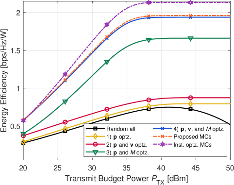
Figure 3: Average EEvs the transmit power budget at the BS ($P_{{\rm TX}}$). Performance evaluation of the proposed algorithm for four different approaches: 1) only $\mathbf{p}$; 2) $\mathbf{p}$ and $\mathbf{v}$; 3) $\mathbf{p}$ and $M$; and 4) $\mathbf{p}$, $\mathbf{v}$ and $M$ optimization denoted as yellow, red, green, and blue color respectively. Random $\mathbf{p}$, $\mathbf{v}$, and $M$ and the instantaneous optimization strategy are denoted as black and purple, respectively.

Moreover, we adopted the instantaneous CSI-based optimization strategy, for gap-performance comparison purposes, which has been implemented based on Algorithm 1 proposed in [37] represented as purple color curves, which is projected specifically for the scenarios multi-user RIS-aided with ZF system, as the same adopted herein. We also plotted the average instantaneous EE obtained from the proposed statistical CSI-based optimization approach, evaluated from the MCs, and depicted in orange color, in order to highlight the efficacy of the proposed method.

First and foremost, it must be noticed the consistency of the EE computed utilizing the ER lower bound, Eq. (11), which undoubtedly proves that $R_{k}>\widetilde{R}_{k}$. This is evident as the obtained EE MCs curve is slightly higher than the EE evaluated from the ER equation, demonstrating the tightness of the derivation proposed in [19] and affirming the potential of the statistical CSI-based optimization for enhancing EE. Regarding the different strategies for statistical CSI-based optimization, it is evident that the proposed algorithm for strategy 4) can outperform all other strategies with statistical CSI optimization in terms of EE enhancement, achieving a significant improvement by increasing the EE from $\approx 0.74$ bps/Hz/W with the random solution (in the maximum value) to $\approx 1.96$ bps/Hz/W. This translates to a remarkable EE gain of approximately $165\%$. Since it optimizes all variables $\mathbf{p}$, $M$, and $\mathbf{v}$ sequentially, such a result was expected. Besides, given the high value assumed by $M_{\max}$ as in practical RIS-aided mMIMO scenarios, there is a significant probability of obtaining a high value of $M$ in the random realizations for both strategies 1) and 2) as depicted in Fig. 4, and analyzed in details in subsection IV-B. Thus, when $M$ is high, the energy consumption is significantly increased implying poor EE. Accordingly, optimizing $M$ becomes of paramount importance.

A notable trend becomes evident when examining the EE of all schemes, except the Random all strategy. Initially, EE experiences an upward trajectory before stabilizing as the transmit budget power $P_{\rm TX}$ of BS increases. This behavior arises because EE does not inherently exhibit a strict monotonically increasing relationship with the transmit budget power. Therefore, when $P_{\rm TX}\geq 40$ dBm, the algorithm can control any surplus transmit power once it is superfluous as its utilization would compromise EE. This explains why the Random all scheme provides a pronounced decline in EE performance as the transmit budget power scales significantly since this approach deploys all the power available .

Moreover, in Fig. 3, one can infer that the impact of optimizing the RIS phase shifts is not negligible on the attainable EE, even considering the statistical optimization. It is noteworthy that the achieved improvement in scenarios in which the number of active BS antennas $M$ assumes low values (optimized $M$) is considerably greater compared to those scenarios where $M$ assumes high values. This can be readily verified by examining the obtained gain in the EE curve of strategy 1) compared to the curve of strategy 2), as well as in the curve of strategy 3) concerning the curve of strategy 4).

Based on Fig. 3, one can see the potential to achieve higher EE through the statistical CSI optimization approach since this methodology enables us to reduce the overhead associated with the phase shifts optimization during each channel coherence time while maintaining the fixed $\mathbf{v}$ over multiples channel coherence time with a minimal performance loss. As a result, the EE decreases from 2.13 to 1.96 bps/Hz/W, representing a loss of $\approx 7.98\%$, in high power regimes.

IV-B Average Number of Active Antennas

Fig. 4 shows the number of average active antennas $M$ for the optimization strategies 1), 2), 3), and 4), as well as for the Random all scheme. It is noteworthy that strategies Random all, 1), and 2) exhibit a significantly higher average number of active antennas compared to the average number of active antennas in strategies 3) and 4). It occurs due to the random assignment for $M$ in each setup $\mathcal{S}$, and since strategies Random all, 1), and 2) do not optimize $M$, there is a high probability for $M$ to be higher than that in strategies 3) and 4). This finding helps explain why strategies Random all, 1), and 2) attain poor EE as illustrated in Fig. 3, and higher rates as analyzed further ahead in Fig. 7.

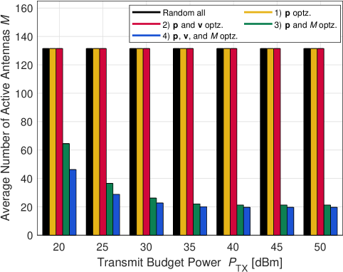
Figure 4: Average number of antennas for four optimization strategies.

Furthermore, by optimizing the RIS phase shifts remarkably reduce the average number of active BS antennas, mainly in low-power regimes, $e.g.$, by comparing strategy 3) with strategy 4), at $P_{{\rm TX}}=20$ dBm, the average number of antennas is reduced from 131 to 46. These results highlight the potential of RIS deployment and optimization.

IV-C Power Consumption

Fig. 5 depicts the average percentage of the transmit power budget utilized for transmission versus the transmit power budget. In the low-budget power regime, all strategies deplete the available power budget; however, as the transmit power budget increases beyond 40 dBm, the algorithm starts to minimize the power consumption. This behavior is expected since aiming to achieve the maximum EE, the available power budget should not be fully utilized.

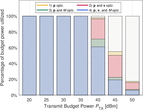
Figure 5: Percentage of the transmit power budget utilized vs the transmit power budget at BS. The colors in the graph are associated with the strategy according to Fig. 3.

Additionally, this strategy is directly accountable for the constant EE observed in high-power budget regimes, as presented in Fig. 3. Furthermore, it becomes apparent that optimizing the number of antennas $M$ is of utmost importance to save a significant amount of power, reducing the power consumption substantially, from $100\%$ (as in the Random all Strategy case) to $61\%$, $19\%$, and $6\%$ in the best strategy, for $P_{{\rm TX}}=$ 40, 45, and 50 dBm respectively. Consequently, this strategy also implies high EE gain, as presented in Fig. 3. Moreover, one can see the substantial impact on power consumption reduction caused by optimizing the RIS phase shifts. This power reduction corroborates the potential of RIS deployment and configuration, resulting in a remarkable EE gain that cannot be obtained in non-RIS scenarios.

IV-D Distribution on the Attainable Data Rates

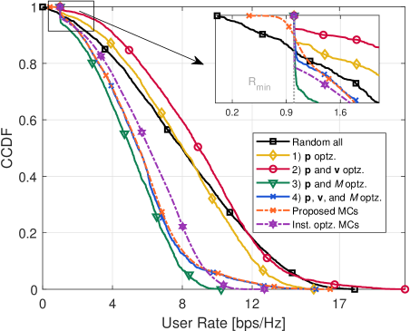
Figure 6: CCDF of the ER $\widetilde{R}_{k}$ for four different strategies with statistical CSI-based optimization (solid lines) and the instantaneous UE rate $R_{k}$ for instantaneous CSI-based optimization (dashed lines), with $R_{\min}$ = 1 bps/Hz.

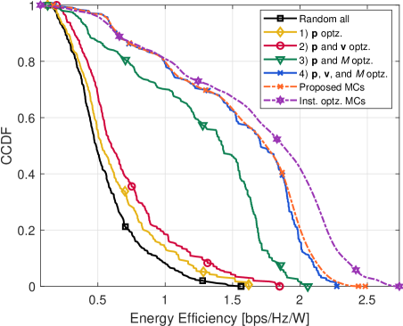
Figure 7: CCDF of the EE for four different optimization strategies with statistical CSI-based optimization (solid lines) and for instantaneous CSI-based optimization (dashed lines), with $R_{\min}=1$ bps/Hz.

Fig. 7 reveals the CCDF of the UE’ ER $\widetilde{R}_{k}$ over $\mathcal{S}=50$ different realizations setups, represented by the solid lines. Besides, dashed lines indicate the computed instantaneous UE’ rate, $R_{k}$, over $\mathcal{T}=500$ MCs for $\mathbf{D}$ and $\mathbf{G}_{{\rm NLoS}}$, in the range of $P_{{\rm TX}}$ from 20 to 50 dBm. Notice that the proposed Statistical CSI-based optimization method necessarily obeys the constraint (18a) for all Strategies solutions. This fulfillment is primordial to guarantee appropriate QoS for all UE s. Moreover, one can see that Strategies Random all, 1), and 2) are capable of providing higher rates than Strategies 3) and 4).

This is due to the consumed power in Strategies 1) and 2) being higher than that in Strategies 3) and 4), as shown in Fig. 5. However, one can see that although Strategy 4) has a much lower number of active antennas and lower power consumption than Strategy 3), Strategy 4) still has a feasible probability of attaining higher rates than Strategy 3). This is due to the RIS phase shifts optimization, which can enhance some UE s by maximizing the ER, as discussed in the subsection III-A. We can also notice from Fig. 7 that the instantaneous UE rate $R_{k}$ obtained through statistical CSI-based optimization (orange dashed curve) can achieve lower rates than $R_{\min}$, implying a violation of (18a), in contrast to the data rates obtained through the instantaneous CSI-based optimization (purple dashed curve), which are always higher or equal than $R_{\min}$.

Additionally, in Fig. 7, we present the CCDF of EE. This graphical representation corroborates that optimization strategies 3) and 4) can effectively fine-tune the number of active antennas and power consumption through the proposed algorithm, leading to enhanced EE at the cost of a tolerable reduction in data rates. Furthermore, it is evident that strategies such as Random all, 1), and 2), where the number of antennas is not optimized, yield lower EE rates. This is attributed to the fact that the majority of setups in $\mathcal{S}$ feature a higher number of active BS antennas in comparison to the active antennas achieved by strategies 3) and 4).

IV-E Rician Coefficient Factor

Fig. 8 illustrates the achievable EE performance as a function of power budget $P_{{\rm TX}}$ for three different Rician factors $K_{1}$. Initially, it becomes evident that in the worst-case scenario, namely when $K_{1}=0$, the greatest disparity between statistical CSI optimization and instantaneous CSI optimization occurs.

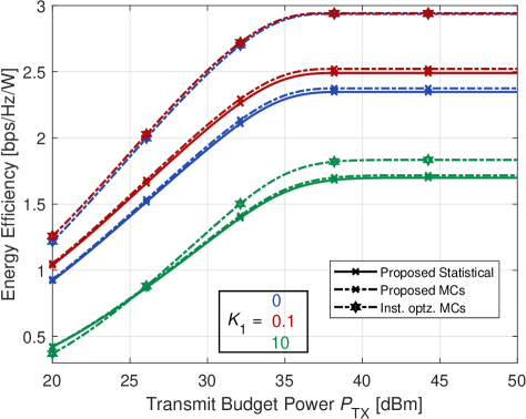
Figure 8: Average EEvs the transmit power budget at the BS ($P_{{\rm TX}}$). Performance evaluation of the proposed algorithm for three different values of Rician factor $K_{1}$.

This observation is justified by considering a scenario with no LoS component for the BS-RIS link. In such a case, optimizing the RIS phase shifts becomes inefficient, where the constants in (12) and (13) reduce, respectively, to $\mathbf{B}=\frac{1}{N}\mathbf{I}_{N}$ and $\mathbf{A}_{k}\approx\frac{1}{N(N\alpha_{G}\alpha_{F,k}+\alpha_{D,k})}\mathbf{I}_{N}$. Therefore, the statistical CSI optimization strategy becomes irrelevant in this scenario. Furthermore, a slight increase in the Rician factor can enhance the system’s performance, underscoring the significant impact of optimizing the RIS phase shifts. However, it becomes apparent that the system’s performance deteriorates when the Rician factor reaches considerably high values. This can be attributed to the dominance of the LoS component in the system, wherein the channel matrix $\mathbf{G}$ becomes rank-deficient, leading to a reduction in multi-path diversity and consequently worsening the overall system performance.

IV-F Computational Complexity of Algorithm 1

In Fig. 9, we illustrate the ER(objective function given by Eq. (11) vs. the average number of iterations ($I_{1}$) attainable with the proposed procedure for RIS phase shifts optimization, Algorithm 1. Additionally, we include a benchmark utilizing the Gradient approach algorithm proposed in [19]. Herein, a backtrack line search strategy for step size determination is adopted, as in [19]. To ensure fairness in our comparison, we apply a consistent stopping criterion for both the proposed algorithm and the gradient-based approach. Specifically, the algorithm will terminate when the absolute difference between the objective function’s values at iterations $n+1$ and $n$, denoted as $f^{(n+1)}$ and $f^{(n)}$ respectively, becomes less than $10^{-3}$, $i.e.$, $|f^{(n+1)}-f^{(n)}|<10^{-3}$. It is apparent that the proposed algorithm achieves a gradual convergence with significantly fewer iterations than the Gradient approach, i.e., the proposed optimization method for both SFP and Analytical strategies needs $I_{1}\approx{20}$ iterations for convergence. Moreover, one can observe that the proposed algorithm outperforms the Gradient approach by achieving $\sum_{k}\widetilde{R}_{k}\approx{42}$ bps/Hz, while the latter achieves around $40$ bps/Hz after 80 iterations.

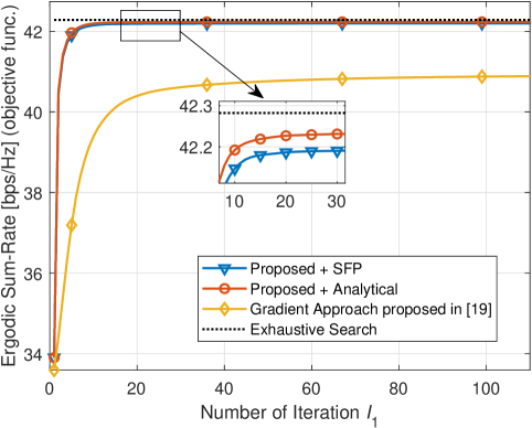
Figure 9: The convergence behavior of the proposed Algorithm 1 for EE maximization and the convergence behavior of the Gradient approach benchmark proposed in [19] over $\mathcal{S}=1000$ different setups. Here we adopt $M=M_{\max}$, $P_{{\rm TX}}=30$ dBm, $K=10$ and $N=25$.

We also can notice in Fig. 9 the potential of the proposed scheme with the SFP method solution since the performance gap is negligible regarding the optimal solution given analytically by Eq. (28), but resulting in a significantly lower complexity according to Table I and III. This clearly highlights the potential of the proposed solution. Furthermore, Table III confirms that the proposed solution with SFP is appealing since the running time is lower than both the Gradient approach and instantaneous CSI-optimization.

TABLE III: Running Time Comparison of the Algorithms in Seconds

	Elapsed Time [s]
Proposed + SFP	0.0287
Proposed + Analytical	0.0572
Gradient Approach [19]	0.0688
Instantaneous CSI Optz.	0.0732

V Conclusions

This work addresses the EE maximization problem in a downlink RIS-aided mMIMO communication system operating under generalized Rician BS-RIS channels and ZF precoding. We proposed a statistical CSI-based optimization strategy that treats the RIS phase shifts and power allocation as a constant over multiple channel coherence time intervals, reducing the overhead of the variables optimization in every channel coherence time. Based on an ER lower-bound closed-form expression, the EE optimization problem with power and QoS constraints is formulated. To circumvent the challenging coupled optimization variables and non-convex constraints, the proposed alternating-sequential optimization approach, based on the fractional programming techniques and dual Lagrangian method, optimizes the power allocation vector ($\bf p$), the number of BS antennas ($M$), and the RIS phase shifts ($\bf v$) in an iterative manner based on analytical closed-form expressions until convergence. Our approach offers an elegant methodology to gradually improve the system EE performance by optimizing the system variables, demonstrating the potential of RIS deployment and optimization in mMIMO systems since the proposed scheme can result in high data rates for the UE s, lower power consumption and lower active antennas operating at BS. Our numerical results validate the effectiveness of the proposed Algorithm, as it substantially reduces the computational complexity while maintaining an exciting trade-off in terms of EE performance. Our approach incurs a performance loss of $\approx 7.98\%$, compared to the instantaneous CSI-based optimization method. Besides, our proposed Algorithm can achieve better EE gains with lower complexity.

Appendix A Proof of Lemma 1

Initially, we should notice the $\mathcal{P}_{3}$ can be equivalently transformed into

$$\max_{\mathbf{v}}\;\mathbf{v}^{H}\mathbf{C}\mathbf{v}=\max_{\mathbf{v}}\;{\rm Tr}\left(\mathbf{C}\mathbf{V}\right),$$ (41)

with $\mathbf{V}=\mathbf{v}\mathbf{v}^{H}$, where the following constraints ${\rm rank}(\mathbf{V})=1$ $[\mathbf{V}]_{n,n}=1$, $\forall n\in\{1,\dots,N\}$, must be attained. Proceeding, conveniently, we can rewritten $\mathbf{v}$ as the following manner

$$\mathbf{v}=[\mathbf{v}_{1}^{H},e^{-j\theta_{n}},\mathbf{v}_{2}^{H}]^{H}.$$ (42)

where $\mathbf{v}_{1}$ $\in\mathbb{C}^{n-1}$ and $\mathbf{v}_{2}$ $\in\mathbb{C}^{N-n}$ are respectively defined as $\mathbf{v}_{1}\triangleq\left[\mathbf{v}\right]_{1:(n-1)}$ and $\mathbf{v}_{2}\triangleq\left[\mathbf{v}\right]_{(n+1):N}$. This alternative notation enables us to look for the $n$-th element of $\mathbf{v}$, $e^{j\theta_{n}}$. Therefore, by utilizing Eq. (42), one can rewrite $\mathbf{V}$ as:

$$\mathbf{V}=\mathbf{v}\mathbf{v}^{H}=\begin{bmatrix}\mathbf{v}_{1}\mathbf{v}_{1}^{H}&\mathbf{v}_{1}e^{-j\theta_{n}}&\mathbf{v}_{1}\mathbf{v}_{2}^{H}\\ e^{j\theta_{n}}\mathbf{v}_{1}^{H}&1&e^{j\theta_{n}}\mathbf{v}_{2}^{H}\\ \mathbf{v}_{2}\mathbf{v}_{1}^{H}&\mathbf{v}_{2}e^{-j\theta_{n}}&\mathbf{v}_{2}\mathbf{v}_{2}^{H}\end{bmatrix}.$$ (43)

By defining the following variables

$$\left\{\begin{aligned} \mathbf{C}_{1}&=\left[\mathbf{C}\right]_{1:(n-1),1:(n-1)}&\quad&\in\mathbb{C}^{(n-1)\times(n-1)}\\ \mathbf{c}_{2}&=\left[\mathbf{C}\right]_{1:(n-1),n}&\quad&\in\mathbb{C}^{(n-1)\times 1}\\ \mathbf{C}_{3}&=\left[\mathbf{C}\right]_{1:(n-1),(n+1):N}&\quad&\in\mathbb{C}^{(n-1)\times(N-n)}\\ C_{4}&=\left[\mathbf{C}\right]_{n,n}&\qquad\quad&\in\mathbb{C}\\ \mathbf{c}_{5}&=\left[\mathbf{C}\right]_{n,(n+1):N}&\quad&\in\mathbb{C}^{1\times(N-n)}\\ \mathbf{C}_{6}&=\left[\mathbf{C}\right]_{(n+1):N,(n+1):N}&\quad&\in\mathbb{C}^{(N-n)\times(N-n)},\end{aligned}\right.$$ (44)

the matrix $\mathbf{C}$ can be rewritten in terms of these variables:

$$\mathbf{C}=\begin{bmatrix}\mathbf{C}_{1}&\mathbf{c}_{2}&\mathbf{C}_{3}\\ \mathbf{c}_{2}^{H}&C_{4}&\mathbf{c}_{5}\\ \mathbf{C}_{3}^{H}&\mathbf{c}_{5}^{H}&\mathbf{C}_{6}\end{bmatrix},$$ (45)

Therefore, after some basic algebraic manipulations:

$${\rm Tr}(\mathbf{C}\mathbf{V}) = e^{-j\theta_{n}}({\rm Tr}(\mathbf{c}_{2}^{H}\mathbf{v}_{1})+{\rm Tr}(\mathbf{c}_{5}\mathbf{v}_{2}))$$

$$+ e^{j\theta_{n}}({\rm Tr}(\mathbf{c}_{2}\mathbf{v}_{1}^{H})+{\rm Tr}(\mathbf{c}_{5}^{H}\mathbf{v}_{2}^{H}))+C_{4}$$

$$+{\rm Tr}\left(\mathbf{C}_{3}\mathbf{v}_{2}\mathbf{v}_{1}^{H}+\mathbf{C}_{1}\mathbf{v}_{1}\mathbf{v}_{1}^{H}+\mathbf{C}_{3}^{H}\mathbf{v}_{1}\mathbf{v}_{2}^{H}\right)+{\rm Tr}\left(\mathbf{C}_{6}\mathbf{v}_{2}\mathbf{v}_{2}^{H}\right),$$

Interestingly, Eq. (A) leads us to see that maximize $\mathcal{P}_{3}$ w.r.t. $\theta_{n}$ is equivalently to

$$\max_{\theta_{n}}\;{\rm Tr}(\mathbf{C}\mathbf{V})=\max_{\theta_{n}}\;2\mathbb{R}\{e^{-j\theta_{n}}({\rm Tr}(\mathbf{c}_{2}^{H}\mathbf{v}_{1})+{\rm Tr}(\mathbf{v}_{2}\mathbf{c}_{5}))\}$$

whose optimal solution is straightforwardly given in closed-form by $\theta_{n}^{\star}=\angle\left({\rm Tr}(\mathbf{c}_{2}^{H}\mathbf{v}_{1})+{\rm Tr}(\mathbf{v}_{2}\mathbf{c}_{5})\right)$. Substituting the values of $\mathbf{c}_{2}$ and $\mathbf{c}_{5}$ given in Eq. (44), and $\mathbf{v}_{1}$ and $\mathbf{v}_{2}$, the proof is complete.

References

- [1] S. Gong, X. Lu, D. T. Hoang, D. Niyato, L. Shu, D. I. Kim, and Y.-C. Liang, “Toward Smart Wireless Communications via Intelligent Reflecting Surfaces: A Contemporary Survey,” IEEE Communications Surveys and Tutorials, vol. 22, no. 4, pp. 2283–2314, 2020.
- [2] Q. Wu and R. Zhang, “Towards Smart and Reconfigurable Environment: Intelligent Reflecting Surface Aided Wireless Network,” IEEE Communications Magazine, vol. 58, no. 1, pp. 106–112, 2020.
- [3] T. Marzetta, E. Larsson, H. Yang, and H. Ngo, Fundamentals of Massive MIMO. Cambridge University Press, 2016.
- [4] W. Jiang, B. Han, M. A. Habibi, and H. D. Schotten, “The Road Towards 6G: A Comprehensive Survey,” IEEE Open Journal of the Communications Society, vol. 2, pp. 334–366, 2021.
- [5] C. D. Alwis, A. Kalla, Q.-V. Pham, P. Kumar, K. Dev, W.-J. Hwang, and M. Liyanage, “Survey on 6G Frontiers: Trends, Applications, Requirements, Technologies and Future Research,” IEEE Open Journal of the Communications Society, vol. 2, pp. 836–886, 2021.
- [6] Y. He, Y. Cai, H. Mao, and G. Yu, “RIS-Assisted Communication Radar Coexistence: Joint Beamforming Design and Analysis,” IEEE Journal on Selected Areas in Communications, vol. 40, no. 7, pp. 2131–2145, July 2022.
- [7] R. Liu, M. Li, Y. Liu, Q. Wu, and Q. Liu, “Joint Transmit Waveform and Passive Beamforming Design for RIS-Aided DFRC Systems,” IEEE Journal of Selected Topics in Signal Processing, vol. 16, no. 5, pp. 995–1010, Aug. 2022.
- [8] J. Kang, H. Wymeersch, C. Fischione, G. Seco-Granados, and S. Kim, “Optimized Switching Between Sensing and Communication for mmWave MU-MISO Systems,” in 2022 IEEE International Conference on Communications Workshops (ICC Workshops), 2022, pp. 498–503.
- [9] W. Lv, J. Bai, Q. Yan, and H. M. Wang, “RIS-Assisted Green Secure Communications: Active RIS or Passive RIS?” IEEE Wireless Communications Letters, vol. 12, no. 2, pp. 237–241, 2023.
- [10] H. Guo, Y.-C. Liang, J. Chen, and E. G. Larsson, “Weighted Sum-Rate Maximization for Reconfigurable Intelligent Surface Aided Wireless Networks,” IEEE Transactions on Wireless Communications, vol. 19, no. 5, pp. 3064–3076, 2020.
- [11] T. Ji, M. Hua, C. Li, Y. Huang, and L. Yang, “Robust Max-Min Fairness Transmission Design for IRS-Aided Wireless Network Considering User Location Uncertainty,” IEEE Transactions on Communications, vol. 71, no. 8, pp. 4678–4693, 2023.
- [12] H. Xie, J. Xu, and Y.-F. Liu, “Max-Min Fairness in IRS-Aided Multi-Cell MISO Systems With Joint Transmit and Reflective Beamforming,” IEEE Transactions on Wireless Communications, vol. 20, no. 2, pp. 1379–1393, 2021.
- [13] T. Jiang and W. Yu, “Interference Nulling Using Reconfigurable Intelligent Surface,” IEEE Journal on Selected Areas in Communications, vol. 40, no. 5, pp. 1392–1406, 2022.
- [14] C. Huang, A. Zappone, G. C. Alexandropoulos, M. Debbah, and C. Yuen, “Reconfigurable Intelligent Surfaces for Energy Efficiency in Wireless Communication,” IEEE Transactions on Wireless Communications, vol. 18, no. 8, pp. 4157–4170, 2019.
- [15] M. Zeng, E. Bedeer, O. A. Dobre, P. Fortier, Q.-V. Pham, and W. Hao, “Energy-Efficient Resource Allocation for IRS-Assisted Multi-Antenna Uplink Systems,” IEEE Wireless Communications Letters, vol. 10, no. 6, pp. 1261–1265, 2021.
- [16] L. You, J. Xiong, D. W. K. Ng, C. Yuen, W. Wang, and X. Gao, “Energy Efficiency and Spectral Efficiency Tradeoff in RIS-Aided Multiuser MIMO Uplink Transmission,” IEEE Transactions on Signal Processing, vol. 69, pp. 1407–1421, 2021.
- [17] M. Forouzanmehr, S. Akhlaghi, A. Khalili, and Q. Wu, “Energy Efficiency Maximization for IRS-Assisted Uplink Systems: Joint Resource Allocation and Beamforming Design,” IEEE Communications Letters, vol. 25, no. 12, pp. 3932–3936, 2021.
- [18] R. K. Fotock, A. Zappone, and M. D. Renzo, “Energy Efficiency in RIS-Aided Wireless Networks: Active or Passive RIS?” 2023.
- [19] K. Zhi, C. Pan, H. Ren, and K. Wang, “Ergodic Rate Analysis of Reconfigurable Intelligent Surface-Aided Massive MIMO Systems With ZF Detectors,” IEEE Communications Letters, vol. 26, no. 2, pp. 264–268, 2022.
- [20] K. Zhi, C. Pan, G. Zhou, H. Ren, and K. Wang, “Analysis and Optimization of RIS-aided Massive MIMO Systems with Statistical CSI,” in 2021 IEEE/CIC International Conference on Communications in China (ICCC Workshops), 2021, pp. 153–158.
- [21] A. Subhash, A. Kammoun, A. Elzanaty, S. Kalyani, Y. H. Al-Badarneh, and M.-S. Alouini, “Optimal Phase Shift Design for Fair Allocation in RIS-Aided Uplink Network Using Statistical CSI,” IEEE Journal on Selected Areas in Communications, vol. 41, no. 8, pp. 2461–2475, 2023.
- [22] C. Yang, K. Yu, and X. Yu, “Energy Efficiency Optimization for Distributed RIS-Assisted MISO System Based on Statistical CSI,” in 2022 IEEE 22nd International Conference on Communication Technology (ICCT), 2022, pp. 875–879.
- [23] H. Ren, X. Liu, C. Pan, Z. Peng, and J. Wang, “Performance Analysis for RIS-Aided Secure Massive MIMO Systems With Statistical CSI,” IEEE Wireless Communications Letters, vol. 12, no. 1, pp. 124–128, 2023.
- [24] E. Björnson and L. Sanguinetti, “Rayleigh Fading Modeling and Channel Hardening for Reconfigurable Intelligent Surfaces,” IEEE Wireless Communications Letters, vol. 10, no. 4, pp. 830–834, 2021.
- [25] E. Björnson, O. T. Demir, and L. Sanguinetti, “A Primer on Near-Field Beamforming for Arrays and Reconfigurable Intelligent Surfaces,” in 2021 55th Asilomar Conference on Signals, Systems, and Computers, 2021, pp. 105–112.
- [26] Y. Han, W. Tang, S. Jin, C.-K. Wen, and X. Ma, “Large Intelligent Surface-Assisted Wireless Communication Exploiting Statistical CSI,” IEEE Transactions on Vehicular Technology, vol. 68, no. 8, pp. 8238–8242, 2019.
- [27] H. Q. Ngo, E. G. Larsson, and T. L. Marzetta, “Energy and Spectral Efficiency of Very Large Multiuser MIMO Systems,” IEEE Transactions on Communications, vol. 61, no. 4, pp. 1436–1449, 2013.
- [28] Z. Yang, M. Chen, W. Saad, W. Xu, M. Shikh-Bahaei, H. V. Poor, and S. Cui, “Energy-Efficient Wireless Communications With Distributed Reconfigurable Intelligent Surfaces,” IEEE Transactions on Wireless Communications, vol. 21, no. 1, pp. 665–679, 2022.
- [29] K. Shen and W. Yu, “Fractional Programming for Communication Systems—Part II: Uplink Scheduling via Matching,” IEEE Transactions on Signal Processing, vol. 66, no. 10, pp. 2631–2644, 2018.
- [30] Y. Jong, “An Efficient Global Optimization Algorithm for Nonlinear Sum-of-Ratios Problem,” Optimization Online, 2012.
- [31] K. Shen and W. Yu, “Fractional Programming for Communication Systems—Part I: Power Control and Beamforming,” IEEE Transactions on Signal Processing, vol. 66, no. 10, pp. 2616–2630, 2018.
- [32] Z.-q. Luo, W.-k. Ma, A. M.-c. So, Y. Ye, and S. Zhang, “Semidefinite Relaxation of Quadratic Optimization Problems,” IEEE Signal Processing Magazine, vol. 27, no. 3, pp. 20–34, 2010.
- [33] H. Li, J. Cheng, Z. Wang, and H. Wang, “Joint Antenna Selection and Power Allocation for an Energy-efficient Massive MIMO System,” IEEE Wireless Communications Letters, vol. 8, no. 1, pp. 257–260, 2019.
- [34] S. Boyd, S. P. Boyd, and L. Vandenberghe, Convex Optimization. Cambridge university press, 2004.
- [35] J. Tang, J. Luo, J. Ou, X. Zhang, N. Zhao, D. K. C. So, and K.-K. Wong, “Decoupling or Learning: Joint Power Splitting and Allocation in MC-NOMA With SWIPT,” IEEE Transactions on Communications, vol. 68, no. 9, pp. 5834–5848, 2020.
- [36] E. Björnson, L. Sanguinetti, J. Hoydis, and M. Debbah, “Optimal Design of Energy-Efficient Multi-User MIMO Systems: Is Massive MIMO the Answer?” IEEE Transactions on Wireless Communications, vol. 14, no. 6, pp. 3059–3075, 2015.
- [37] N. I. Miridakis, T. A. Tsiftsis, and R. Yao, “Zero Forcing Uplink Detection Through Large-Scale RIS: System Performance and Phase Shift Design,” IEEE Transactions on Communications, vol. 71, no. 1, pp. 569–579, 2023.