Multi-Higgs Boson Production with Anomalous Interactions at Current and Future Proton Colliders

Abstract

We investigate multi-Higgs boson production at proton colliders, in a framework involving anomalous interactions, focusing on triple Higgs boson production. We consider modifications to the Higgs boson self-couplings, to the Yukawa interactions, as well as new contact interactions of Higgs bosons with either quarks or gluons. To this end, we have developed a MadGraph5_aMC@NLO loop model, publicly available at gitlabrepo, designed to incorporate the relevant operators in the production of multiple Higgs bosons (and beyond). We have performed cross section fits at various energies over the anomalous interactions, and have derived constraints on the most relevant anomalous coefficients, through detailed phenomenological analyses at proton-proton collision energies of 13.6 TeV and 100 TeV, through the 6 $b$-jet final state.

1 Introduction

Measuring the interactions of the Higgs boson Higgs:1964pj; Englert:1964et; Guralnik:1964eu; ATLAS:2012yve; CMS:2012qbp with the rest of the Standard Model (SM), with itself (i.e. its self-interactions), and with potential new phenomena, is a crucial task for future collider experiments. There are multiple theoretical justifications for the importance of the Higgs field and how it interacts; for example, the Higgs doublet bilinear, $H^{\dagger}H$, is the only dimension-2 ($D=2$) singlet operator within the SM. This kind of operator readily allows for $D=3$ or $D=4$ interactions with one, or two, new scalar singlet fields, that may constitute part of a “hidden sector” of hitherto undetected particles. Therefore, the Higgs boson could be our primary window to this, potentially “dark”, sector, that could comprise part, or all, of dark matter. Another reason of the importance of the Higgs boson’s interactions is that they may illuminate the mechanism of baryogenesis – in particular, if this process occurred during the electro-weak phase transition, the period during which the Higgs field acquires a vacuum expectation value (VEV), then the Higgs field may be one of the protagonists of electro-weak baryogenesis (see, e.g. Dorsch:2013wja; No:2013wsa; Curtin:2014jma; Profumo:2014opa; White:2016nbo; Basler:2016obg; Bernon:2017jgv; Kurup:2017dzf; Dorsch:2017nza; Ramsey-Musolf:2019lsf; Li:2019tfd; Papaefstathiou:2020iag; Papaefstathiou:2021glr; Papaefstathiou:2022oyi; Zuk:2022qwx). A central rôle in this mechanism is played by the Higgs potential, which, within the SM, is introduced in rather ad-hoc manner. The form of this potential can, in principle, be directly probed by measuring the Higgs boson’s self-interactions through multi-Higgs boson production processes: the triple self-coupling can be probed through Higgs boson pair production, and the quartic through triple production.

Novel Higgs boson interactions, to new or to SM particles, may arise at the electro-weak scale, but they may also appear at higher scales, $\mathcal{O}(\mathrm{few~{}TeV})$. If this is the case, we can parametrize our ignorance using a higher-dimensional effective field theory (EFT), see, e.g. Buchmuller:1985jz; Grzadkowski:2010es; Elias-Miro:2013mua. Neglecting lepton-number violating operators, the lowest-dimensionality EFT that can be written down consists of $D=6$ operators. Upon electro-weak symmetry breaking, the Higgs boson would acquire a VEV and these operators would result in several new interactions, as well modifications of the SM interactions of the Higgs boson. Several of the operators in the physical basis of the Higgs boson scalar ($h$) would then have coefficients that are correlated, according to $D=6$ EFT. These correlations, however, may be broken by even higher-dimensional operators (e.g. $D=8$), particularly if the new phenomena are closer to the electro-weak scale. Therefore, it may be beneficial to lean towards a more agnostic, and hence more phenomenological, approach and, while still remaining inspired by $D=6$ EFT, consider fully uncorrelated, “anomalous” interactions of the Higgs boson with the SM. This is the approach that we pursue here.

Within the realm of self-coupling measurements, and beyond, Higgs boson pair production has received considerable attention from both the experimental (e.g. CMS:2017yfv; CMS:2017hea; CMS:2017rpp; CMS:2018tla; CMS:2018vjd; CMS:2018sxu; CMS:2018ipl; CMS:2020tkr; CMS:2022cpr; CMS:2022hgz; CMS:2022kdx; CMS:2022omp; ATLAS:2014pjm; ATLAS:2015zug; ATLAS:2015sxd; ATLAS:2016paq; ATLAS:2018rnh; ATLAS:2018dpp; ATLAS:2018hqk; ATLAS:2018uni; ATLAS:2018fpd; ATLAS:2018ili; ATLAS:2019qdc; ATLAS:2019vwv; ATLAS:2020jgy; ATLAS:2021ifb; ATLAS:2022xzm; ATLAS:2022jtk; ATLAS:2023qzf; ATLAS:2023gzn) and theoretical (e.g. Baur:2002rb; Baur:2002qd; Baur:2003gp; Dolan:2012ac; Papaefstathiou:2012qe; Cao:2013si; Goertz:2013kp; Arbey:2013jla; deFlorian:2013uza; Gupta:2013zza; Ellwanger:2013ova; Barr:2013tda; Maierhofer:2013sha; deFlorian:2013jea; Dolan:2013rja; Goertz:2013eka; Frederix:2014hta; Baglio:2014nea; FerreiradeLima:2014qkf; deFlorian:2014rta; Hespel:2014sla; Barger:2014taa; Godunov:2014waa; Liu:2014rba; Maltoni:2014eza; Chen:2014ask; Barr:2014sga; MartinLozano:2015vtq; Papaefstathiou:2015iba; Dawson:2015oha; Kotwal:2015rba; Lu:2015jza; Carvalho:2015ttv; Batell:2015koa; Dawson:2015haa; Cao:2015oaa; Kanemura:2016tan; Contino:2016spe; Banerjee:2016nzb; Huang:2017jws; Nakamura:2017irk; Lewis:2017dme; DiLuzio:2017tfn; Grober:2017gut; Zurita:2017sfg; Arganda:2017wjh; Adhikary:2017jtu; Bauer:2017cov; Maltoni:2018ttu; Borowka:2018pxx; Goncalves:2018qas; Chang:2018uwu; Basler:2018dac; Adhikary:2018ise; DiMicco:2019ngk; Cheung:2020xij) point of view, particularly following the discovery of the Higgs boson. Owing to its much smaller SM cross section at hadron colliders Maltoni:2014eza, triple Higgs boson has understandably received much less attention. To the extent of our knowledge, it was first investigated in Plehn:2005nk, where it was demonstrated that the prospects for the measurement of the quartic self-coupling will be very challenging, both at the LHC and a future ‘VLHC’ at a center-of-mass energy of 200 TeV. Subsequent studies of triple Higgs boson production at future colliders Papaefstathiou:2015paa; Chen:2015gva; Fuks:2015hna; Papaefstathiou:2017hsb; Fuks:2017zkg; Liu:2018peg; Papaefstathiou:2019ofh; deFlorian:2019app; Chiesa:2020awd; Abdughani:2020xfo, with the knowledge of the Higgs boson mass, and the prospects for Higgs boson pair production measurements at hand, further quantified the difficulty of this measurement, nevertheless demonstrating that some useful information may be obtained via the process. The situation at LHC energies is much more dire, as expected, requiring either new phenomena for sufficient enhancement Papaefstathiou:2020lyp, or very large new contributions to the Higgs boson’s self-interactions Stylianou:2023xit. Up to now, all of the phenomenological studies addressing triple Higgs boson production, apart from discussions of the cross section modifications in an EFT in Degrande:2020evl, have considered only the effects of modifications of the self-couplings. However, due to their loop-induced nature, proceeding via heavy quark loops, multi-Higgs boson production processes are highly sensitive to modifications of the heavy quark Yukawa couplings, as well as to additional quark- or gluon-Higgs boson contact interactions that generically arise in EFTs. Such effects have been studied within the context of Higgs boson pair production, see, e.g. Goertz:2014qta; Azatov:2015oxa. In the present article we study, for the first time to the best of our knowledge, the combined effect of modifications to the self-couplings, Yukawa interactions, and new heavy-quark- or gluon-Higgs boson contact interactions in triple Higgs boson production, within the aforementioned EFT-inspired anomalous coupling picture. To achieve this, we have constructed a specialized anomalous-coupling model within the MadGraph5_aMC@NLO event generator that incorporates the full interference effects between contributing diagrams.

The paper is organized as follows: in section 2 we introduce the phenomenological Lagrangian that we employ in our study, inspired by the $D=6$ EFT extension of the SM. In section 3 we discuss the details of the Monte Carlo implementation of the MadGraph5_aMC@NLO model, briefly addressing its usage for Higgs boson pair and triple production. In section 4 we discuss our phenomenological analysis of triple Higgs boson production, focusing on cross section fits, existing constraints on the anomalous couplings, and the extraction of limits on the most relevant coefficients through the 6 $b$-jet final state. We present our conclusions and outlook in section 5. In addition, in appendix A we describe the $D=6$ EFT phenomenological Lagrangian relevant to Higgs boson production processes, and in appendix B we discuss aspects of the validation of the Monte Carlo model. In appendix C we discuss relevant Feynman diagrams that appear within our framework, and in appendix D we present supplementary cross section fits at various proton collision energies.

2 Phenomenological Lagrangian

To allow for additional freedom, we have modified the $D=6$ EFT Lagrangian relevant to Higgs boson processes, derived in detail in appendix A (eq. 20), breaking the correlations between several of the interactions that originate in the $D=6$ EFT. This yields more flexibility when exploring multi-Higgs boson production experimentally. Nevertheless, $D=6$ EFT can be trivially restored by reinstating the appropriate relations between the coefficients (see below).

To achieve this, we have defined new anomalous couplings $d_{3}$ and $d_{4}$, as modifications of the triple and quartic self-couplings, $c_{g1}$ and $c_{g2}$ as interactions of two gluons and one or two Higgs bosons, respectively, and $c_{f1}$, $c_{f2}$ and $c_{f3}$ as interactions between fermion-anti-fermion pairs, and one, two or three Higgs bosons, respectively, leading to the following phenomenological Lagrangian:

$$\begin{split}\mathcal{L}_{\mathrm{Pheno}}=&-\frac{m_{h}^{2}}{2v}\left(1+d_{3}\right)h^{3}-\frac{m_{h}^{2}}{8v^{2}}\left(1+d_{4}\right)h^{4}\\ &+\frac{\alpha_{s}}{4\pi}\left(c_{g1}\frac{h}{v}+c_{g2}\frac{h^{2}}{2v^{2}}\right)G_{\mu\nu}^{a}G^{\mu\nu}_{a}\\ &-\left[\frac{m_{t}}{v}\left(1+c_{t1}\right)\bar{t}_{L}t_{R}h+\frac{m_{b}}{v}\left(1+c_{b1}\right)\bar{b}_{L}b_{R}h+\text{h.c.}\right]\\ &-\left[\frac{m_{t}}{v^{2}}\left(\frac{3c_{t2}}{2}\right)\bar{t}_{L}t_{R}h^{2}+\frac{m_{b}}{v^{2}}\left(\frac{3c_{b2}}{2}\right)\bar{b}_{L}b_{R}h^{2}+\text{h.c.}\right]\\ &-\left[\frac{m_{t}}{v^{3}}\left(\frac{c_{t3}}{2}\right)\bar{t}_{L}t_{R}h^{3}+\frac{m_{b}}{v^{3}}\left(\frac{c_{b3}}{2}\right)\bar{b}_{L}b_{R}h^{3}+\text{h.c.}\right].\end{split}$$ (1)

To recover the $D=6$ EFT Lagrangian relevant to the Higgs sector (i.e. eq. 20), one would need to simply set: $d_{3}=c_{6}$, $d_{4}=6c_{6}$, $c_{g1}=c_{g2}$, $c_{f1}=c_{f2}=c_{f3}$.

The implementation of this study further modifies the above phenomenological Lagrangian to match more closely the LHC experimental collaboration definitions:

$$\begin{split}\mathcal{L}_{\mathrm{PhenoExp}}=&-\lambda_{\mathrm{SM}}v\left(1+d_{3}\right)h^{3}-\frac{\lambda_{\mathrm{SM}}}{4}\left(1+d_{4}\right)h^{4}\\ &+\frac{\alpha_{s}}{12\pi}\left(c_{g1}\frac{h}{v}-c_{g2}\frac{h^{2}}{2v^{2}}\right)G_{\mu\nu}^{a}G^{\mu\nu}_{a}\\ &-\left[\frac{m_{t}}{v}\left(1+c_{t1}\right)\bar{t}_{L}t_{R}h+\frac{m_{b}}{v}\left(1+c_{b1}\right)\bar{b}_{L}b_{R}h+\text{h.c.}\right]\\ &-\left[\frac{m_{t}}{v^{2}}c_{t2}\bar{t}_{L}t_{R}h^{2}+\frac{m_{b}}{v^{2}}c_{b2}\bar{b}_{L}b_{R}h^{2}+\text{h.c.}\right]\\ &-\left[\frac{m_{t}}{v^{3}}\left(\frac{c_{t3}}{2}\right)\bar{t}_{L}t_{R}h^{3}+\frac{m_{b}}{v^{3}}\left(\frac{c_{b3}}{2}\right)\bar{b}_{L}b_{R}h^{3}+\text{h.c.}\right],\end{split}$$ (2)

where we have taken $\lambda_{\mathrm{SM}}\equiv m_{h}^{2}/2v^{2}$.

The CMS parametrization is then obtained by setting: $\kappa_{\lambda}=(1+d_{3})$, $k_{t}=c_{t1}$, $c_{2}=c_{t2}$, $c_{g}=c_{g1}$, $c_{gg}=c_{2g}$ and the ATLAS parametrization by $c_{hhh}=(1+d_{3})$, $c_{ggh}=2c_{g1}/3$, $c_{gghh}=-c_{g2}/3$. The Lagrangian of eq. 2 encapsulates the form of the interactions that we employ for the rest of our phenomenological analysis.

3 Monte Carlo Event Generation

3.1 Loop $\times$ Tree-Level Interference

The implementation of the Lagrangian of eq. 2 in MadGraph5_aMC@NLO (MG5_aMC) Alwall:2011uj; Hirschi:2015iia follows closely the instructions for proposed code modifications found in loopxtree. These modifications essentially introduce tree-level diagrams in the form of “UV counter-terms”, that are generated along with any loop-level diagrams, allowing the calculation of interference terms between them. The model of the present article, created through this procedure, has been fully validated by direct comparison to an implementation of Higgs boson pair production in $D=6$ EFT in the HERWIG 7 Monte Carlo, and by taking the limit of a heavy scalar boson for those vertices that do not appear in that process. See appendix B for further details of the latter effort. The necessary modifications to the MG5_aMC codebase, as well as the model can be found in the public gitlab repository at gitlabrepo.

3.2 Higgs Boson Pair Production

Higgs boson pair production contains a subset of all diagrams relevant to triple Higgs boson production, minus one Higgs boson insertion, and therefore we begin by investigating this process, so as to provide a simple example.

MG5_aMC allows for calculation of the interference terms via one insertion of the operator at the squared matrix-element level ($|\mathcal{M}|^{2}$):

generate g g > h h [noborn=MHEFT QCD] MHEFT^2<=1

i.e. schematically: $|\mathcal{M}|^{2}\sim\bullet 1+\sqbullet c_{i}$. The classes of diagrams that are included in addition to the SM ones (fig. LABEL:fig:hh_sm), are those that appear in fig. LABEL:fig:eft1insert, found in appendix C.

Alternatively, one can obtain: the interference terms of one or two insertions with the SM, and the squares of one-insertion terms (equivalent to two powers of the anomalous couplings) via:

generate g g > h h [noborn=MHEFT QCD] MHEFT^2<=2

where schematically this would correspond to $|\mathcal{M}|^{2}\sim\bullet 1+\sqbullet c_{i}+\star c_{i}c_{j}$. The classes of diagrams of fig. LABEL:fig:eft2insert (appendix C) appear in addition.

3.3 Triple Higgs Boson Production

For the investigation of triple Higgs boson production, which constitutes the focus of this article, we included the interference terms of one or two insertions with the SM and the squares of one-insertion terms through:

generate g g > h h h [noborn=MHEFT QCD] MHEFT^2<=2

As for Higgs boson pair production, this would schematically correspond to $|\mathcal{M}|^{2}\sim\bullet 1+\sqbullet c_{i}+\star c_{i}c_{j}$. The classes of the various diagrams that appear are shown in fig. LABEL:fig:hhh_sm for the SM, and in figs. LABEL:fig:eft1insert_hhh for one insertion, and LABEL:fig:eft2insert_hhh for two insertions, in appendix C.

4 Phenomenology of Triple Higgs Boson Production

4.1 Cross Section Fits

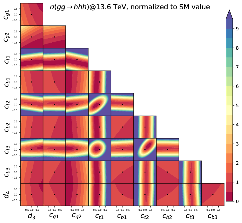
Figure 2: Fit of the cross section for triple Higgs boson production at 13.6 TeV, normalized to the SM value. For each combination of couplings, the other couplings have been set to zero for simplicity. Each change of color in the contours represents a shift of a factor of 0.5$\times$ the SM value.

By employing our Monte Carlo implementation of eq. 2, We have performed cross section fits at a proton-proton collider at 13, 13.6, 14, 27, and 100 TeV, over all coefficients relevant to either Higgs boson pair or triple production. Two-dimensional projections of the fits for $E_{\mathrm{CM}}=13.6$ TeV appear in fig 2 for triple production. In this figure, for each corresponding plot, all other coefficients have been set to zero, for the sake of simplicity.

cccccccccccc[hvlines,corners=NE] $d_{3}$ & -0.750 0.292
$d_{4}$ -0.158 -0.0703 0.0340
$c_{g1}$ -0.278 0.0426 0.0484 0.0256
$c_{g2}$ 1.39 -0.704 -0.0312 -0.156 0.538
$c_{t1}$ 6.94 -3.17 -0.309 -0.850 5.16 12.6
$c_{t2}$ -3.61 4.05 -0.872 -0.0482 -4.15 -17.6 15.3
$c_{t3}$ -2.72 -1.57 1.33 0.906 -0.316 -4.64 -18.2 13.0
$c_{b1}$ -0.125 0.177 -0.0457 -0.00903 -0.166 -0.675 1.38 -0.941 0.0317
$c_{b2}$ 0.106 -0.0752 0.00692 -0.00740 0.0949 0.433 -0.509 0.162 -0.0219 0.00489
$c_{b3}$ 0.161 -0.0809 -0.00396 -0.0182 0.124 0.598 -0.474 -0.0434 -0.0189 0.0109 0.00719
1 $d_{3}$ $d_{4}$ $c_{g1}$ $c_{g2}$ $c_{t1}$ $c_{t2}$ $c_{t3}$ $c_{b1}$ $c_{b2}$ $c_{b3}$

Table 1: Polynomial coefficients, $A_{i}$ (second column only) and $B_{ij}$, relevant for the determination of the cross section for leading-order Higgs boson triple production, in the form $\sigma/\sigma_{\mathrm{SM}}-1=A_{i}c_{i}+B_{ij}c_{i}c_{j}$, where $c_{i}\in\left\{d_{3},c_{g1},c_{g2},c_{t1},c_{t2},c_{b1},c_{b2},\right\}$, at $E_{\mathrm{CM}}=13.6~{}\mathrm{TeV}$.

The numerical values of the coefficients, in the form $\sigma/\sigma_{\mathrm{SM}}-1=A_{i}c_{i}+B_{ij}c_{i}c_{j}$, where $c_{i}\in\left\{d_{3},d_{4},c_{g1},c_{g2},c_{t1},c_{t2},c_{t3},c_{b1},c_{b2},c_{b3}\right\}$, are shown for $E_{\mathrm{CM}}=13.6$ TeV in table 1 for triple production. For Higgs boson pair production at $E_{\mathrm{CM}}=13.6~{}\mathrm{TeV}$, see table 7, in appendix D. The coefficients for both processes, at $E_{\mathrm{CM}}=13,~{}14,~{}27$ and $100$ TeV can be found in appendix D. The table should be read as follows: each value shown corresponds to the coefficient multiplying the product of the couplings of the corresponding first column and last row, respectively. As an example, with reference to table 1, the coefficient of the term proportional to $d_{4}d_{3}$ is $-0.0703$, i.e. read off the second row, third column. Using these coefficients, one can construct the cross section for any given value of the anomalous couplings.

All the fits for the signal processes, and subsequent simulations, have been performed using the MSHT20nlo_as118 PDF set Bailey:2020ooq and the default dynamical scale choice (option 3) in MG5_aMC, which corresponds to the sum of the transverse mass divided by 2.

4.2 Other Constraints on Anomalous Couplings

The majority of the anomalous couplings that appear in the phenomenological Lagrangian of eq. 2 are already tightly constrained by other processes that involve the interactions of gluons, top and bottom quarks with the Higgs boson. The two exceptions that are not presently constrained are the anomalous interactions of three Higgs bosons and two top or bottom quarks, with relevant coefficients $c_{t3}$ and $c_{b3}$, as well as the anomalous modification to the Higgs boson’s quartic interaction, related to the $d_{4}$ coefficient. While it is beyond the scope of the present study to perform a full fit, involving several processes and constraints, it is important to provide order-of-magnitude estimates for the two scenarios that we examine: the 13.6 TeV high-luminosity LHC, and the 100 TeV FCC-hh at the end of its lifetime.

cccc[hvlines,corners=NE]   Percentage uncertainties  
HL-LHC FCC-hh Ref.
$\delta(d_{3})$ 50 5 deBlas:2019rxi (table 12)
$\delta(c_{g1})$ 2.3 0.49 deBlas:2019rxi (table 3)
$\delta(c_{g2})$ 5 1 Azatov:2015oxa (Figure 12, right)
$\delta(c_{t1})$ 3.3 1.0 deBlas:2019rxi (table 3)
$\delta(c_{t2})$ 30 10 Azatov:2015oxa (Figure 12, right)
$\delta(c_{b1})$ 3.6 0.43 deBlas:2019rxi (table 3)
$\delta(c_{b2})$ 30 10 Azatov:2015oxa (Figure 12, right)

Table 2: Estimates of percentage uncertainties (%) obtained on the subset of anomalous couplings that appear in other processes at the HL-LHC and FCC-hh. The last column provides the source for these numbers.

We consider the constraints on $c_{t1}$, $c_{b1}$ and $c_{g1}$ that would arise within the “kappa-0” scenario, as they are defined in deBlas:2019rxi (table 3). For the HL-LHC we consider those labeled “HL-LHC”, and for the 100 TeV FCC-hh, we consider those projected after the combined results of “FCC-ee240+FCC-ee365”, “FCC-eh”, and “FCC-hh” for the FCC-hh, collectively labeled “FCC-ee/eh/hh”. For the modifications to the Higgs boson triple self-coupling, we use the values quoted for the “di-Higgs exclusive” results for the “HL-LHC”, shown in table 12 of deBlas:2019rxi. For $c_{g2}$, $c_{t2}$ and $c_{b2}$, we assume approximate constraints derived from the results of the analysis of Azatov:2015oxa. For all the coefficients, we assume that the central value of these future measurements will be at zero. The assumed constraints are summarized as percentage uncertainties in table 4.2, along with the corresponding references, for convenience.

4.3 Statistical Analysis

The goal of the present phenomenological analysis is two-fold: on the one hand, we wish to determine if triple Higgs boson production itself can be observed at the end of the HL-LHC or FCC-hh lifetime, and on the other, we wish to calculate the constraints that would be obtained on the anomalous couplings, given the assumption the SM is the true underlying theory. The first goal corresponds to the null hypothesis being the absence of triple Higgs boson production, whereas the latter corresponds to the null hypothesis being SM triple Higgs boson production, i.e. triple production with all the anomalous coupling coefficients set to zero.

For the first of these goals, i.e. to determine the significance, $\Sigma$, of observing triple Higgs boson production for a certain anomalous coupling parameter-space point, we optimize the signal versus background discrimination according to the phenomenological analysis described in the next section (4.4), to obtain the maximum significance over the set of cuts for SM triple Higgs boson production. Since we expect the number of signal events to be much lower than that for the background, we employ the following formula for the significance:

$$\Sigma=\frac{S}{\sqrt{B+(\alpha B)^{2}}}\;,$$ (3)

where $S$ and $B$ are the expected number of signal and background events, respectively, at a given integrated luminosity $\mathcal{L}$, and $\alpha$ is a factor that we employ to model the systematic uncertainty present in the background estimation. During our search for the maximum SM triple Higgs boson production significance, we used the value $\alpha=0$, i.e. we optimized $S/\sqrt{B}$. Subsequently, all results are presented with this optimal set of cuts, obtained at a given collider, while setting the systematic uncertainty factor $\alpha=0.05$.

We have derived the expected “evidence” (3$\sigma$) and “discovery” (5$\sigma$) limits on the observation of triple Higgs boson production on the $(c_{t3},d_{4})$-plane, where the novel information coming from triple Higgs boson production is expected to arise. Furthermore, we have derived the 68% confidence level (C.L.) (1$\sigma$) and 95% C.L. (2$\sigma$) expected limits on the same plane, given that the SM hypothesis is true. While doing so, we allow the coefficients $d_{3}$ and $c_{t2}$ to vary. These will be constrained primarily via Higgs boson pair production, and since this is a challenging process in itself, will not be substantially constrained compared to the gluon-Higgs anomalous interactions, or the top-anti-top-Higgs anomalous coupling, $c_{t1}$, see table 4.2 for a quantification of this statement. In addition, we do not expect triple Higgs boson production to be competitive to Higgs boson pair production in terms of constraints on $d_{3}$ and $c_{t2}$, so we “marginalize” over these two.

To derive the evidence and discovery limits for triple Higgs boson production, we assume that the number of signal and background events follow gaussian distributions, and define the uncertainty on the background number of events as:

$$\delta_{\mathrm{B}}=\sqrt{B+(\alpha B)^{2}}\;.$$ (4)

Then, the probability value ($p$-value) to obtain a given number of signal events, $S(\{c_{i}\})$, corresponding to the set of anomalous coupling coefficients $\{c_{i}\}$, is given by:

$$P(\{c_{i}\})=\frac{1}{\sqrt{2\pi}\delta_{\mathrm{B}}}\exp\left[-\frac{S(\{c_{i}\})^{2}}{2\delta_{\mathrm{B}}^{2}}\right]\;.$$ (5)

To take into account the approximate constraints of table 4.2, that would be present, ignoring possible correlations that will exist between constraints, we multiply the $p$-values by a gaussian prior factor:

$$P_{C}(c_{i})=\frac{1}{\sqrt{2\pi}\delta(c_{i})}\exp\left[-\frac{c_{i}^{2}}{2\delta(c_{i})^{2}}\right]\;,$$ (6)

at a value $c_{i}$ of each of the anomalous coefficients $d_{3}$ and $c_{t2}$. We then marginalize by integrating over the $d_{3}$ and $c_{t2}$ directions. Since this is done over a grid, the integral is represented by a sum over the grid points:

$$P_{M}(c_{t3},d_{4})=\sum_{(d_{3},c_{t2})}\Delta d_{3}\Delta c_{t2}P_{C}(d_{3})P_{C}(c_{t2})P(\{c_{i}\})\;,$$ (7)

where $\Delta d_{3}$ and $\Delta c_{t2}$ are the bin widths in the $d_{3}$ and $c_{t2}$ directions, respectively. The probability is then converted to $\chi^{2}$ via the Python $\chi^{2}$ inverse survival function for two degrees of freedom (scipy.stats.chi2.isf), and the 3$\sigma$ and 5$\sigma$ limits are found by drawing the iso-contours corresponding to $\chi^{2}-\chi^{2}_{\mathrm{min}}=(11.8,28.7)$, respectively. The results are shown in Fig. 3, in section 4.5.

For the determination of the constraints obtained for the null hypothesis being SM triple Higgs boson production, we folow a similar procedure. In this scenario, we assume that the number of events for both signal and background follow a gaussian distribution, as we did before, and hence the uncertainty on the number of total expected SM events is given by:

$$\delta_{\mathrm{SM+B}}=\sqrt{S_{\mathrm{SM}}+B+(\alpha B)^{2}}\;,$$ (8)

where $S_{\mathrm{SM}}$ represents the expected number of events for SM triple Higgs boson production. Then the $p$-value to obtain a given number of events corresponding to an anomalous coupling parameter-space point, $S(\{c_{i}\})$, given that the SM is the truth, is given by:

$$\bar{P}(\{c_{i}\})=\frac{1}{\sqrt{2\pi}\delta_{\mathrm{SM+B}}}\exp\left[-\frac{(S_{\mathrm{SM}}-S(\{c_{i}\}))^{2}}{2\delta_{\mathrm{SM+B}}^{2}}\right]\;.$$ (9)

This $p$-value is then multiplied by the prior factors of eq. 6, and summed as before:

$$\bar{P}_{M}(c_{t3},d_{4})=\sum_{(d_{3},c_{t2})}\Delta d_{3}\Delta c_{t2}P_{C}(d_{3})P_{C}(c_{t2})\bar{P}(\{c_{i}\})\;,$$ (10)

followed by a conversion to the $\chi^{2}$ value as before. The 68% (1$\sigma$) and 95% (2$\sigma$) confidence level (C.L.) intervals are found by drawing the iso-contours corresponding to $\chi^{2}-\chi^{2}_{\mathrm{min}}=(2.28,5.99)$, respectively. The results of this analysis are shown in Fig. 4, in section 4.5.

To obtain the one-dimensional limits on either of the $d_{4}$ or $c_{t3}$ couplings alone, we take the procedure one step further: we sum over the additional marginalized coupling as in eq. 10, and convert the $p$-value into a $\chi^{2}$ value. For the triple Higgs boson searches, we calculate the $3\sigma$ and $5\sigma$ evidence and discovery limits by finding the points that correspond to $\chi^{2}-\chi^{2}_{\mathrm{min}}=(9.00,25.0)$, respectively. For the expected constraints on the $d_{4}$ and $c_{t3}$ coefficients, given that the SM is true, we calculate the $1\sigma$ and $2\sigma$ intervals by finding the points that correspond to $\chi^{2}-\chi^{2}_{\mathrm{min}}=(0.99,3.84)$, respectively. The results for the evidence and discovery points, and for the expected limits given that the SM is true, are shown in tables 5 and 6, respectively, in section 4.5

4.4 Phenomenological Analysis

To obtain constraints on anomalous triple Higgs boson production at proton colliders, following the statistical procedure outlined above, we have performed a hadron-level phenomenological analysis of the 6 $b$-jet final-state originating from the decays of all three Higgs bosons to $b\bar{b}$ quark pairs. We closely follow the analysis of Refs. Papaefstathiou:2019ofh; Papaefstathiou:2020lyp. Parton-level events have been generated using the MG5_aMC anomalous couplings implementation constructed in the present article, with showering, hadronization, and simulation of the underlying event, performed via the general-purpose HERWIG 7 Monte Carlo event generator Bahr:2008pv; Gieseke:2011na; Arnold:2012fq; Bellm:2013hwb; Bellm:2015jjp; Bellm:2017bvx; Bellm:2019zci; Bewick:2023tfi. The event analysis was performed via the HwSim framework addon to HERWIG 7 hwsim. No smearing due to the detector resolution or identification efficiencies have been applied to the final objects used in the analysis, apart from a $b$-jet identification efficiency, discussed below.

The branching ratio of $h\rightarrow b\bar{b}$ will be modified primarily due to $c_{t1}$, $c_{g1}$, indirectly through modifications to the $h\rightarrow gg$ and $h\rightarrow\gamma\gamma$ branching ratios, and directly through $c_{b1}$. To take this effect into account, we employed the eHDECAY code Contino:2014aaa. The program eHDECAY includes QCD radiative corrections, and next-to-leading order EW corrections are only applied to the SM contributions. For further details, see Ref. Contino:2014aaa. We have performed a fit of the eHDECAY branching ratio $h\rightarrow b\bar{b}$, and we have subsequently normalized this to the latest branching ratio provided by the Higgs Cross Section Working Group’s Yellow Report yr4page; LHCHiggsCrossSectionWorkingGroup:2016ypw, $\mathrm{BR}(h\rightarrow b\bar{b})=0.5824$. The fit is then used to rescale the final cross section of $pp\rightarrow hhh\rightarrow(b\bar{b})(b\bar{b})(b\bar{b})$. The background processes containing Higgs bosons turned out to be subdominant with respect to the dominant QCD 6 $b$-jet and $Z$+jets backgrounds, and therefore we did not modify these when deriving the final cross sections.

For the generation of the backgrounds involving $b$-quarks not originating from either a $Z$ or Higgs boson, we imposed the following generation-level cuts for the 100 TeV proton collider: $p_{T,b}>30~{}\mathrm{GeV}$, $|\eta_{j}|<5.0$, and $\Delta R_{b,b}>0.2$. The transverse momentum cut was lowered to $p_{T,b}>20~{}\mathrm{GeV}$ for 13.6 TeV, except for the QCD 6 $b$-jet background, for which we produced the events inclusively, without any generation cuts. The selection analysis was optimized considering as a main backgrounds the QCD-induced process $pp\rightarrow(b\bar{b})(b\bar{b})(b\bar{b})$, and the $Z$+jets process (represented by $Z+(b\bar{b})(b\bar{b})$), which we found to be significant at LHC energies.

The event selection procedure for our analyses proceeds as follows: as in Papaefstathiou:2019ofh, an event is considered if there are at least six $b$-tagged jets, of which only the six ones with the highest $p_{T}$ are taken into account. A universal minimal threshold for the transverse momentum, $p_{T,b}$, of any of the selected $b$-tagged jets is imposed. In addition a universal cut on their maximum pseudo-rapidity, $|\eta_{b}|$, is also applied. We subsequently make use of the observable:

$$\chi^{2,(6)}=\sum_{qr\in I}(m_{qr}-m_{h})^{2}\;,$$ (11)

where $I=\{jb_{1}jb_{2},jb_{3}jb_{4},jb_{5}jb_{6}\}$ is the set of all possible 15 pairings of 6-$b$ tagged jets. Out of all the possible combinations we pick the one with the smallest value $\chi_{\rm min}^{2,(6)}$. The pairings of $b$-jets defining $\chi_{\rm min}^{2,(6)}$ constitute our best candidates for the reconstruction of the three Higgs bosons, $h$. Our studies have demonstrated that $\chi_{\rm min}^{2,(6)}$ is one of the most powerful observables to employ in signal versus background discrimination.

We further refine the discrimination power of the $\chi_{\rm min}^{2,(6)}$ variable by using the individual mass differences $\Delta m=|m_{qr}-m_{h}|$ in eq. (11), sorting them out according to $\Delta m_{\rm min}<\Delta m_{\rm med}<\Delta m_{\rm max}$, and imposing independent cuts on each of them. We also consider the transverse momentum $p_{T}(h^{i})$ of each reconstructed Higgs boson candidate. These reconstructed particles are also sorted based on the value of $p_{T}(h^{i})$, on which we then impose a cut. Besides the universal minimal threshold on $p_{T,b}$, introduced at the beginning of this section, we impose cuts on the three $b$-jets with the highest transverse momentum $p_{T,b_{i}}$, for $i=1,2,3$. The set of cuts $p_{T,b_{3}}<p_{T,b_{2}}<p_{T,b_{1}}$ is the second most powerful discriminating observable in our list. Finally, we also considered two additional geometrical observables. The first of them is the distance between $b$-jets in each reconstructed Higgs boson $\Delta R_{bb}(h^{i})$. The second one is the distance between the reconstructed Higgs bosons $\Delta R(h^{i},h^{j})$ themselves.

Our optimization process then proceeds as in Papaefstathiou:2019ofh; Papaefstathiou:2020lyp: we sequentially try different combination of cuts over the observables introduced above on our signal and background samples until we achieve a significance above $2$ or when our number of Monte Carlo events is reduced so drastically that no meaningful statistical conclusions can be derived if this number becomes smaller (this happens for instance when for a given combination of cuts, we are left with less than 10 Monte Carlo events of signal or background).

Optimized cuts
Observable	$13.6$ TeV	$100$ TeV
$p_{T,b}>$	$25.95$ GeV	$35.00$ GeV
$|\eta_{b}|<$	$2.3$	$3.3$
$\Delta R_{bb}>$	$0.3$	$0.3$
$p_{T,b_{i}}>$	$[25.95,25.95,25.95]$ GeV $i=1,2,3$	$[170.00,135.00,35.00]$ GeV
$\chi^{2,(6)}<$	$27.0$ GeV	$26.0$ GeV
$\Delta m_{\rm{min,med,max}}<$	$[100,200,300]$ GeV	$[8,8,8]$ GeV
$\Delta R_{bb}(h^{i})<$	$[3.5,3.5,3.5]$	$[3.5,3.5,3.5]$
$\Delta R(h^{i},h^{j})<$	$[3.5,3.5,3.5]$	$[3.5,3.5,3.5]$
$p_{T}(h^{i})>$	$[0.0,0.0,0.0]$ GeV	$[200.0,190.0,20.0]$ GeV
$p_{T\rm jet}>$	$25$ GeV	$25$ GeV
$|\eta_{\rm jet}|<$	$4.0$	$4.0$

Table 3: Optimized cuts determined for the phenomenological analysis. The indices $i,j$ can take the values $i,j=1,2,3$. For the cut $\Delta R(h^{i},h^{j})$ the three pairings correspond to $(1,2),(1,3),(2,3)$. The indexed elements should be read from left to right in increasing order. The last two rows refer to cuts over light jets.

LHC Analysis $(13.6~{}\rm{TeV})$
Process	$\sigma_{\rm{NLO}}(6~{}b\mathrm{-jet})~{}[\rm{fb}]$	$\varepsilon_{\rm{analysis}}$	$N^{\rm{cuts}}_{3\times 10^{3}~{}\rm{fb}^{-1}}$
$hhh(\rm{SM})$	$1.97\times 10^{-2}$	$0.12$	$2.77$
QCD $(b\bar{b})(b\bar{b})(b\bar{b})$	6136.12	$1.00\times 10^{-5}$	69.67
$pp\rightarrow Z(b\bar{b})(b\bar{b})$	61.80	0.0045	318.17
$pp\rightarrow ZZ(b\bar{b})$	2.16	0.0059	14.3
$pp\rightarrow hZ(b\bar{b})$	0.45	0.0159	8.1
$pp\rightarrow hhZ$	0.0374	0.034	1.45
$pp\rightarrow hh(b\bar{b})$	0.0036	0.028	0.11
LI $gg\rightarrow hZZ$	0.143	0.022	3.62
LI $gg\rightarrow ZZZ$	0.124	0.013	1.76
LI $gg\rightarrow hhZ$	0.0458	0.047	2.42
FCC-hh Analysis $(100~{}\rm{TeV})$
Process	$\sigma_{\rm{NLO}}(6~{}b\mathrm{-jet})~{}[\rm{fb}]$	$\varepsilon_{\rm{analysis}}$	$N^{\rm{cuts}}_{20~{}\rm{ab}^{-1}}$
$hhh(\rm{SM})$	$1.14$	$0.0115$	$98.90$
QCD $(b\bar{b})(b\bar{b})(b\bar{b})$	$56.66\times 10^{3}$	$1.12\times 10^{-5}$	4777.71
$pp\rightarrow Z(b\bar{b})(b\bar{b})$	1285.37	$3.04\times 10^{-5}$	294.63
$pp\rightarrow ZZ(b\bar{b})$	49.01	$2.02\times 10^{-5}$	7.48
$pp\rightarrow hZ(b\bar{b})$	9.87	$3.04\times 10^{-5}$	2.26
$pp\rightarrow hhZ$	0.601	$5.95\times 10^{-4}$	2.70
$pp\rightarrow hh(b\bar{b})$	0.096	$8.095\times 10^{-5}$	$\ll 1$
LI $gg\rightarrow hZZ$	8.28	$1.62\times 10^{-4}$	$10.12$
LI $gg\rightarrow ZZZ$	6.63	$4.05\times 10^{-5}$	$2.03$
LI $gg\rightarrow hhZ$	2.65	$2.54\times 10^{-4}$	5.07

Table 4: The lists of processes considered during our phenomenological analysis, along with their respective cross sections to the 6 $b$-jet final state. The efficiencies $\varepsilon_{\rm analysis}$ and number of events $N_{\mathcal{L}}^{\rm cuts}$, correspond to those obtained after applying the set of cuts given in table 3. A $b$-jet identification efficiency of $0.85$ (for each $b$-jet) has also been applied to obtain the number of events. For the HL-LHC we considered an integrated luminosity of $\mathcal{L}=3000~{}\hbox{fb}^{-1}$, and for for the FCC-hh a luminosity of $\mathcal{L}=20~{}\hbox{ab}^{-1}$. To approximate higher-order corrections, a $K$-factor $K=2$ has been included for all processes, with respect to the leading-order cross section. The background processes marked with “LI” represent loop-induced contributions that have been generated separately.

For $100~{}\rm{TeV}$, the observables are optimized in the following order, (i) $p_{T,b}$, (ii) $|\eta_{b}|$, (iii) $\chi^{2,(6)}$, (iv) $\Delta m_{\rm min}$, $\Delta m_{\rm med}$, $\Delta m_{\rm max}$, (v) $p_{T,b_{1}}$ and (vi) $p_{T,b_{2}}$. By testing different cut combinations over the variables above we reach a SM triple Higgs boson significance of $S/\sqrt{B}\simeq 2.33\sigma$ without $b$-jet tagging or $S/\sqrt{B}\simeq 1.43\sigma$ including the $b$-tagging factor (0.85). We note that this is an improvement over the previous result of Papaefstathiou:2019ofh, where the corresponding significance was around $1.7\sigma$ without $b$-tagging. For $13.6~{}\rm{TeV}$ the optimization of the cuts follows a similar path, however after applying the cut on $\chi^{2,(6)}$ we are left with $\mathcal{O}(10)$ Monte Carlo events for background, and therefore the full procedure stops at a significance of only $0.23\sigma$ without $b$-jet tagging or $0.14\sigma$ with $b$-jet tagging ($0.85$). The concrete values of the cuts applied on the different kinematic variables depend on the center of mass energy of the collider under study, and are summarized on table 3. We note that the optimal set of cuts for the HL-LHC requires more central $b$-jets than that at the FCC-hh. The complete list of backgrounds, their initial cross sections, efficiency of cuts and expected number of events at each of the full collider luminosities, are given in table 4. It is interesting to note that the $Z+(b\bar{b})(b\bar{b})$ is in fact the dominant one at the HL-LHC, whereas the reverse is true for the FCC-hh. It will be important to validate this result in a future detailed experimental study that consider the full effects of the detectors.

To employ the results of the SM analysis over the whole of the parameter space we are considering, we have performed a polynomial fit of the efficiency of the analysis on the signal, $\varepsilon_{\mathrm{analysis}}(hhh)$, at various, randomly-chosen, combinations of anomalous coefficient values. In combination with the fits of the cross section, and the fit of the branching ratio of the Higgs boson to $(b\bar{b})$, we can estimate the number of events at a given luminosity, for a given collider for any parameter-space point within the anomalous coupling picture, which we dubbed $S(\{c_{i}\})$ in our discussion of the statistical approach we take, in section 4.3.

4.5 Results

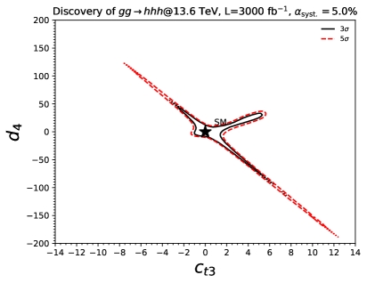
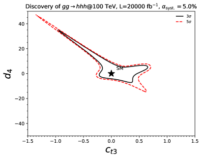
Figure 3: The 3$\sigma$ evidence (black solid) and 5$\sigma$ discovery (red dashed) curves on the $(c_{t3},d_{4})$-plane for triple Higgs boson production at 13 TeV/3000 fb${}^{-1}$ (left), and 100 TeV/20 ab${}^{-1}$ (right), marginalized over the $c_{t2}$ and $d_{3}$ anomalous couplings. Note the differences in the axes ranges at each collider.

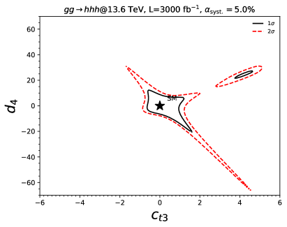
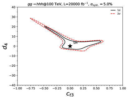
Figure 4: The 68% C.L. (1$\sigma$, black solid) and 95% C.L (2$\sigma$, red dashed) limit on the $(c_{t3},d_{4})$-plane for triple Higgs boson production at 13 TeV/3000 fb${}^{-1}$ (left), and 100 TeV/20 ab${}^{-1}$ (right), marginalized over the $c_{t2}$ and $d_{3}$ anomalous couplings. Note the differences in the axes ranges at each collider.

ccc——cc[hvlines,corners=NE] & HL-LHC 3$\sigma$ HL-LHC 5$\sigma$ FCC-hh 3$\sigma$ FCC-hh 5$\sigma$
$d_{4}$ $[-28,0,41.7]$ $[-99.5,152.9]$ $[-24.9,20.8]$ $[-40.8,23.1]$
$c_{t3}$ $[-2.1,5.5]$ $[-7.1,11.3]$ $[-0.8,0.6]$ $[-1.2,0.7]$

Table 5: The 3$\sigma$ evidence and 5$\sigma$ discovery limits on for triple Higgs boson production, for the $c_{t3}$ and $d_{4}$ coefficients at 13 TeV/3000 fb${}^{-1}$, and 100 TeV/20 ab${}^{-1}$, marginalized over $c_{t2}$, $d_{3}$ and either $d_{4}$, or $c_{t3}$.

ccc——cc[hvlines,corners=NE] & HL-LHC 68% HL-LHC 95% FCC-hh 68% FCC-hh 95%
$d_{4}$ $[-6.6,12.4]$ $[-10.0,21.3]$ $[-3.9,10.5]$ $[-10.6,18.8]$
$c_{t3}$ $[-0.6,1.1]$ $[-0.9,3.6]$ $[-0.1,0.3]$ $[-0.4,0.6]$

Table 6: The 68% C.L. (1$\sigma$) and 95% C.L (2$\sigma$) limits on $c_{t3}$ and $d_{4}$ for triple Higgs boson production at 13 TeV/3000 fb${}^{-1}$, and 100 TeV/20 ab${}^{-1}$, marginalized over $c_{t2}$, $d_{3}$ and either $d_{4}$, or $c_{t3}$.

The main results of our two-dimensional analysis over the $(c_{t3},d_{4})$-plane are shown in figs. 3 and 4. In particular, fig. 3 shows the potential “evidence” and “discovery” regions (3$\sigma$ and 5$\sigma$, respectively) for triple Higgs boson production at the high-luminosity LHC on the left (13.6 TeV with 3000 fb${}^{-1}$ of integrated luminosity), and at a FCC-hh (100 TeV, with 20 ab${}^{-1}$) on the right. Evidently, very large modifications to the quartic self-coupling are necessary for discovery of triple Higgs boson production at the HL-LHC, ranging from $d_{4}\sim 125$ for $c_{t3}~{}\sim-8$, to $d_{4}\sim\pm 40$ for $c_{t3}\sim 0$ and then down to $d_{4}\sim-200$ for $c_{t3}\sim 12$. The situation is greatly improved, as expected, at the FCC-hh, where the range of $d_{4}$ is reduced to $d_{4}~{}\sim 40$ for $c_{t3}\sim-1.5$, and to $d_{4}\sim-20$ for $c_{t3}\sim 1.0$. It is interesting to note that the whole of the parameter space with $c_{t3}\gtrsim 1.0$, or with $c_{t3}\lesssim-1.5$ is discoverable, at the FCC-hh at 5$\sigma$. For the potential 68% (1$\sigma$) and 95% C.L. (2$\sigma$) constraints of fig. 4, the situation is slightly more encouraging for the HL-LHC, with the whole region of $d_{4}\gtrsim 40$ or $d_{4}\lesssim-60$ excluded at 95% C.L.. The corresponding region at 68% C.L. is $d_{4}\gtrsim 20$ and $d_{4}\lesssim-30$. For $c_{t3}$, it is evident that all the region $c_{t3}\lesssim-2$ and $c_{t3}\gtrsim 5$ will be excluded at 95% C.L. and $c_{t3}\lesssim-1$, $c_{t3}\gtrsim 4$ at 68% C.L.. On the other hand, the FCC-hh will almost be able to exclude the whole positive region of $d_{4}$ for any value of $c_{t3}$ at 68% C.L.. This will potentially be achievable if combined with other Higgs boson triple production final states. For the $c_{t3}$ coupling, both the constraints reach the $\mathcal{O}(\mathrm{few}~{}10\%)$ level for any value of $d_{4}$.

The one-dimensional analysis’ results, presented in tables 5 and 6, for the “evidence” and “discovery” potential, and exclusion limits, respectively, reflect the above conclusions. For instance, it is clear by examining table 5, that the HL-LHC will only see evidence of triple Higgs boson production in the 6 $b$-jet final state only if $d_{4}$ has modifications of $|d_{4}|\sim\mathcal{O}(\mathrm{few}~{}10)$, and will only discover it if $|d_{4}|\sim\mathcal{O}(100)$. On the other hand, there could be evidence or discovery of Higgs boson triple production if $|c_{t3}|\sim\mathcal{O}(\mathrm{1-10})$. The 1$\sigma$ and 2$\sigma$ exclusion regions are much tighter, as expected, with $|d_{4}|\sim\mathcal{O}(10)$ at 1$\sigma$ or 2$\sigma$ at the HL-LHC, improving somewhat at the FCC-hh, and $|c_{t3}|\sim\mathcal{O}(0.1-1)$, both at the HL-LHC and FCC-hh.

5 Conclusions

We have conducted a phenomenological analysis of the triple Higgs boson production at the high-luminosity LHC (13.6 TeV with 3000 fb${}^{-1}$) and a proposed future circular collider colliding protons at 100 TeV (20 ab${}^{-1}$). For this analysis, we have constructed a model to be used with the MadGraph5_aMC@NLO event generator, which is publicly available at gitlabrepo. By examining the 6 $b$-jet final state, within a signal versus background analysis, we have concluded that interesting constraints can be obtained on the most relevant coefficients, $d_{4}$ and $c_{t3}$, representing modifications to the Higgs quartic self-coupling, and additional top-Higgs interactions, respectively. These are presented, for the HL-LHC and the FCC-hh, over the $(c_{t3},d_{4})$-plane in figs. 3 and 4, showing the evidence/discovery potential of the triple Higgs boson production process itself, marginalized over the $d_{3}$ and $c_{t2}$ coefficients, and the 1/2$\sigma$ exclusion regions arising from the process on that plane. The one-dimensional evidence/discovery regions over either $d_{4}$, or $c_{t3}$ at both colliders are given in table 5, and the possible constraints extracted in table 6.

The results of our study demonstrate the importance of including additional contributions, beyond the modifications to the self-couplings, when examining multi-Higgs boson production processes, and in particular triple Higgs boson production. We are looking forward to a more detailed study for the HL-LHC, conducted by the ATLAS and CMS collaborations, including detector simulation effects, and the full correlation between other channels. From the phenomenological point of view, improvements will arise by including additional final states, e.g. targetting the process $pp\rightarrow hhh\rightarrow(b\bar{b})(b\bar{b})(\tau^{+}\tau^{-})$, or by performing an analysis that leverages machine learning techniques to maximize significance. In summary, we believe that the triple Higgs boson production process should constitute part of a full multi-dimensional fit, within the anomalous couplings picture.

Appendix A $D=6$ Effective Field Theory

The phenomenological Lagrangian employed in this study has been inspired by the $D=6$ effective field theory (EFT) Lagrangian of ref. Goertz:2014qta.

The terms contributing to multi-Higgs production via gluon fusion at the LHC at $D=6$ EFT are:

$$\begin{split}\mathcal{L}_{h^{n}}=&-\mu^{2}|H|^{2}-\lambda|H|^{4}-\left(y_{t}\bar{Q}_{L}H^{c}t_{R}+y_{b}\bar{Q}_{L}Hb_{R}+\text{h.c.}\right)\\ &+\frac{c_{H}}{2\Lambda^{2}}(\partial^{\mu}|H|^{2})^{2}-\frac{c_{6}}{\Lambda^{2}}\lambda_{\mathrm{SM}}|H|^{6}+\frac{\alpha_{s}c_{g}}{4\pi\Lambda^{2}}|H|^{2}G_{\mu\nu}^{a}G^{\mu\nu}_{a}\\ &-\left(\frac{c_{t}}{\Lambda^{2}}y_{t}|H|^{2}\bar{Q}_{L}H^{c}t_{R}+\frac{c_{b}}{\Lambda^{2}}y_{b}|H|^{2}\bar{Q}_{L}Hb_{R}+\text{h.c.}\right),\end{split}$$ (12)

where the first line includes the relevant Standard Model terms that will receive corrections from $D=6$ operators. For the purposes of the current study, we set $C_{H}=0$ in what follows. We also assume minimal flavour violation DAmbrosio:2002vsn, which leads to the coefficients of the Yukawa-like terms in the last row of eq. 12 being proportional to the (SM-like) Yukawa couplings.

Examining the relevant terms in the scalar potential and expanding about the electro-weak minimum, we get:

$$\mathcal{L}_{\mathrm{self}}= - \mu^{2}\frac{(v+h)^{2}}{2}-\lambda\frac{(v+h)^{4}}{4}-\frac{c_{6}\lambda_{\mathrm{SM}}}{\Lambda^{2}}\frac{(v+h)^{6}}{8}$$

$$= - \frac{\mu^{2}}{2}(v^{2}+2hv+h^{2})-\frac{\lambda}{4}(v^{4}+4hv^{3}+6h^{2}v^{2}+4h^{3}v+h^{4})$$ (13)

$$- \frac{c_{6}\lambda_{\mathrm{SM}}}{8\Lambda^{2}}(v^{6}+6v^{5}h+15v^{4}h^{2}+20h^{3}v^{3}+15v^{2}h^{4}+6h^{5}v+h^{6})\;.$$

Omitting terms with $h^{n}$, $n>4$, and constant terms we arrive at

$$\mathcal{L}_{\mathrm{self}}= - \frac{\mu^{2}}{2}(2hv+h^{2})-\frac{\lambda}{4}(4hv^{3}+6h^{2}v^{2}+4h^{3}v+h^{4})$$ (14)

$$- \frac{c_{6}\lambda_{\mathrm{SM}}}{8\Lambda^{2}}(6hv^{5}+15h^{2}v^{4}+20h^{3}v^{3}+15h^{4}v^{2})+~{}...\;.$$

Finally, we focus on the fermion-Higgs boson interactions that receive contributions from

$$\mathcal{L}_{hf}=-\frac{y_{f}}{\sqrt{2}}\bar{f}_{L}(h+v)f_{R}-\frac{c_{f}y_{f}}{\Lambda^{2}}\frac{(v+h)^{2}}{2}\bar{f}_{L}\frac{(v+h)}{\sqrt{2}}f_{R}\,+\text{h.c.}\;,$$ (15)

where $f=t,b,~{}...$, with $f_{L,R}$ the left- and right-handed fields, and the first term comes from the SM whereas the second term is a dimension-6 contribution. Expanding, we obtain

$$\mathcal{L}_{hf}= - \frac{y_{f}v}{\sqrt{2}}\left(1+\frac{c_{t}v^{2}}{2\Lambda^{2}}\right)\bar{f}_{L}f_{R}$$ (16)

$$- \frac{y_{f}}{\sqrt{2}}\left(1+\frac{3c_{f}v^{2}}{2\Lambda^{2}}\right)\bar{f}_{L}f_{R}h$$

$$- \frac{y_{f}}{\sqrt{2}}\left(\frac{3c_{f}v}{2\Lambda^{2}}\right)\bar{f}_{L}f_{R}h^{2}$$

$$- \frac{y_{f}}{\sqrt{2}}\left(\frac{c_{f}}{2\Lambda^{2}}\right)\bar{f}_{L}f_{R}h^{3}\,+\text{h.c.}\;.$$

The first line gives the expression for the modified fermion mass,

$$m_{f}=\frac{y_{f}v}{\sqrt{2}}\left(1+\frac{c_{t}v^{2}}{2\Lambda^{2}}\right)\,,$$ (17)

and we can re-express eq. (16) in terms of this:

$$\mathcal{L}_{hf}= - m_{f}\bar{f}_{L}f_{R}$$ (18)

$$- \frac{m_{f}}{v}\left(1+\frac{c_{f}v^{2}}{\Lambda^{2}}\right)\bar{f}_{L}f_{R}h$$

$$- \frac{m_{f}}{v}\left(\frac{3c_{f}v}{2\Lambda^{2}}\right)\bar{f}_{L}f_{R}h^{2}$$

$$- \frac{m_{f}}{v}\left(\frac{c_{f}}{2\Lambda^{2}}\right)\bar{f}_{L}f_{R}h^{3}\,+\text{h.c.}\;.$$

The final term that we need to consider is

$$\mathcal{L}_{hg} = \frac{\alpha_{s}c_{g}}{4\pi\Lambda^{2}}|H|^{2}G_{\mu\nu}^{a}G^{\mu\nu}_{a}$$ (19)

$$= \frac{\alpha_{s}c_{g}}{4\pi\Lambda^{2}}\frac{(h+v)^{2}}{2}G_{\mu\nu}^{a}G^{\mu\nu}_{a}$$

$$= \frac{\alpha_{s}c_{g}}{4\pi\Lambda^{2}}(hv+\frac{h^{2}}{2})G_{\mu\nu}^{a}G^{\mu\nu}_{a}+~{}...\;,$$

where the omitted constant term can be absorbed into an unobservable re-definition of the gluon wave function.

We thus obtain the following interactions in terms of the Higgs boson scalar $h$, relevant to Higgs boson multi-production:

$$\begin{split}\mathcal{L}_{\mathrm{D=6}}=&-\frac{m_{h}^{2}}{2v}\left(1+c_{6}\right)h^{3}-\frac{m_{h}^{2}}{8v^{2}}\left(1+6c_{6}\right)h^{4}\\ &+\frac{\alpha_{s}c_{g}}{4\pi}\left(\frac{h}{v}+\frac{h^{2}}{2v^{2}}\right)G_{\mu\nu}^{a}G^{\mu\nu}_{a}\\ &-\left[\frac{m_{t}}{v}\left(1+c_{t}\right)\bar{t}_{L}t_{R}h+\frac{m_{b}}{v}\left(1+c_{b}\right)\bar{b}_{L}b_{R}h+\text{h.c.}\right]\\ &-\left[\frac{m_{t}}{v^{2}}\left(\frac{3c_{t}}{2}\right)\bar{t}_{L}t_{R}h^{2}+\frac{m_{b}}{v^{2}}\left(\frac{3c_{b}}{2}\right)\bar{b}_{L}b_{R}h^{2}+\text{h.c.}\right]\\ &-\left[\frac{m_{t}}{v^{3}}\left(\frac{c_{t}}{2}\right)\bar{t}_{L}t_{R}h^{3}+\frac{m_{b}}{v^{3}}\left(\frac{c_{b}}{2}\right)\bar{b}_{L}b_{R}h^{3}+\text{h.c.}\right],\end{split}$$ (20)

where we have explicitly written down the contributing components of the $Q_{L}$ doublets.

Appendix B Validation of the Monte Carlo Implementation

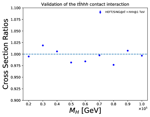
Figure 6: The ratio of cross sections between for $t\bar{t}\rightarrow hhh$ between the anomalous interaction (HEFT) and the heavy scalar ($H$) descriptions. See main text for further details.

Almost all vertices relevant in triple Higgs boson production are present in pair production. Therefore, these were validated using the HiggsPair model in HERWIG 7 Monte Carlo event generator, with minor modifications, in the $gg\rightarrow hh$ process. Validation of the new $t\bar{t}hhh$ contact interaction was performed by considering the processes $t\bar{t}\rightarrow hhh$ at 1 TeV in the $t\bar{t}$ center-of-mass frame without a PDF involved. The processes were calculated both in the HEFT and in a model with a heavy scalar ($H$) that couples to $t\bar{t}$ and $hhh$ only. This implies taking the limit of the effective field theory directly and checking whether the effective vertex functions as expected. The matching of the coefficient of eq. 2 with the singlet model, e.g. of Papaefstathiou:2020iag, implies that $c_{t3}=2v^{2}/M_{H}^{2}$, when the the quartic coupling between the heavy scalar and the three Higgs bosons is set to $\lambda_{1112}=1$ and the mixing angle $\theta=\pi/2$ such that the SM Higgs boson is decoupled. Figure 6 shows the ratio of the anomalous $t\bar{t}hhh$ interaction cross section over the heavy scalar cross section for various masses of the heavy scalar, chosen to be much higher than the center-of-mass energy.

Appendix C Feynman Diagrams

Figures LABEL:fig:eft1insert and LABEL:fig:eft2insert represent the Feynman diagrams for either one or two insertions of the operators used in the present article in Higgs boson pair production. Figures LABEL:fig:eft1insert_hhh and LABEL:fig:eft2insert_hhh represent the Feynman diagrams for either one or two insertions in the context of Higgs boson triple production.

Appendix D Cross Section Fits for Triple and Double Higgs Boson Production at Various Energies

ccccccccc[hvlines, corners = NE] $d_{3}$ & -0.786 0.181
$c_{g1}$ -0.386 0.0412 0.150
$c_{g2}$ 0.971 -0.123 -0.715 0.853
$c_{t1}$ 4.86 -1.87 -1.02 2.56 5.91
$c_{t2}$ -5.57 1.70 2.08 -5.06 -13.9 10.0
$c_{b1}$ -0.0900 -0.0656 0.224 -0.526 -0.298 1.17 0.0964
$c_{b2}$ 0.0629 0.0668 -0.199 0.468 0.224 -1.01 -0.174 0.0786
1 $d_{3}$ $c_{g1}$ $c_{g2}$ $c_{t1}$ $c_{t2}$ $c_{b1}$ $c_{b2}$

Table 7: Polynomial coefficients, $A_{i}$ (second column only) and $B_{ij}$, relevant for the determination of the cross section for leading-order Higgs boson pair production, in the form $\sigma/\sigma_{\mathrm{SM}}-1=A_{i}c_{i}+B_{ij}c_{i}c_{j}$, where $c_{i}\in\left\{d_{3},c_{g1},c_{g2},c_{t1},c_{t2},c_{b1},c_{b2},\right\}$, at $E_{\mathrm{CM}}=13.6~{}\mathrm{TeV}$.

ccccccccc[hvlines, corners = NE] $d_{3}$ & -0.846 0.179
$c_{g1}$ -0.385 0.164 0.406
$c_{g2}$ 1.03 -0.438 -1.07 0.777
$c_{t1}$ 4.92 -2.08 -1.63 3.34 6.37
$c_{t2}$ -5.85 2.48 3.09 -5.32 -16.2 11.2
$c_{b1}$ -0.00554 0.00287 0.244 -0.289 -0.238 0.662 0.0400
$c_{b2}$ -0.0117 0.00464 -0.138 0.159 0.101 -0.339 -0.0461 0.0133
1 $d_{3}$ $c_{g1}$ $c_{g2}$ $c_{t1}$ $c_{t2}$ $c_{b1}$ $c_{b2}$

Table 8: Polynomial coefficients, $A_{i}$ (second column only) and $B_{ij}$, relevant for the determination of the cross section for leading-order Higgs boson pair production, in the form $\sigma/\sigma_{\mathrm{SM}}-1=A_{i}c_{i}+B_{ij}c_{i}c_{j}$, where $c_{i}\in\left\{d_{3},c_{g1},c_{g2},c_{t1},c_{t2},c_{b1},c_{b2},\right\}$, at $E_{\mathrm{CM}}=13~{}\mathrm{TeV}$.

cccccccccccc[hvlines,corners=NE] $d_{3}$ & -0.824 0.225
$d_{4}$ -0.147 -0.0640 0.0755
$c_{g1}$ -0.229 0.123 -0.0151 0.0168
$c_{g2}$ 1.35 -0.609 -0.0411 -0.168 0.470
$c_{t1}$ 6.76 -3.22 -0.00692 -0.888 4.78 12.3
$c_{t2}$ -3.82 3.24 -1.59 0.864 -3.37 -19.5 16.1
$c_{t3}$ -2.76 -0.384 1.92 -0.0730 -1.16 -3.36 -17.6 12.4
$c_{b1}$ -0.121 0.167 -0.123 0.0440 -0.137 -0.871 2.00 -1.45 0.0661
$c_{b2}$ 0.0382 -0.0607 0.0478 -0.0159 0.0470 0.306 -0.748 0.566 -0.0501 0.00950
$c_{b3}$ 0.0676 -0.0445 0.0137 -0.0120 0.0535 0.294 -0.378 0.135 -0.0217 0.00804 0.00239
1 $d_{3}$ $d_{4}$ $c_{g1}$ $c_{g2}$ $c_{t1}$ $c_{t2}$ $c_{t3}$ $c_{b1}$ $c_{b2}$ $c_{b3}$

Table 9: Polynomial coefficients, $A_{i}$ (second column only) and $B_{ij}$, relevant for the determination of the cross section for leading-order Higgs boson triple production, in the form $\sigma/\sigma_{\mathrm{SM}}-1=A_{i}c_{i}+B_{ij}c_{i}c_{j}$, where $c_{i}\in\left\{d_{3},c_{g1},c_{g2},c_{t1},c_{t2},c_{b1},c_{b2},\right\}$, at $E_{\mathrm{CM}}=13~{}\mathrm{TeV}$.

ccccccccc[hvlines, corners = NE] $d_{3}$ & -0.857 0.282
$c_{g1}$ -0.386 0.291 0.0772
$c_{g2}$ 0.957 -1.08 -0.613 1.38
$c_{t1}$ 5.00 -2.38 -1.12 3.20 6.39
$c_{t2}$ -5.86 3.50 1.76 -6.17 -15.8 11.0
$c_{b1}$ -0.0500 0.165 0.101 -0.514 -0.298 0.865 0.0529
$c_{b2}$ -0.00429 -0.0655 -0.0420 0.228 0.0704 -0.324 -0.0489 0.0115
1 $d_{3}$ $c_{g1}$ $c_{g2}$ $c_{t1}$ $c_{t2}$ $c_{b1}$ $c_{b2}$

Table 10: Polynomial coefficients, $A_{i}$ (second column only) and $B_{ij}$, relevant for the determination of the cross section for leading-order Higgs boson pair production, in the form $\sigma/\sigma_{\mathrm{SM}}-1=A_{i}c_{i}+B_{ij}c_{i}c_{j}$, where $c_{i}\in\left\{d_{3},c_{g1},c_{g2},c_{t1},c_{t2},c_{b1},c_{b2},\right\}$, at $E_{\mathrm{CM}}=14~{}\mathrm{TeV}$.

cccccccccccc[hvlines,corners=NE] $d_{3}$ & -0.827 0.414
$d_{4}$ -0.211 -0.110 0.0511
$c_{g1}$ -0.208 0.210 -0.0282 0.0265
$c_{g2}$ 1.28 -0.700 -0.0655 -0.177 0.440
$c_{t1}$ 6.67 -3.57 -0.372 -0.901 4.55 11.8
$c_{t2}$ -3.73 4.96 -0.993 1.26 -3.59 -18.2 15.5
$c_{t3}$ -2.67 -2.19 1.61 -0.558 -0.551 -3.38 -18.1 12.9
$c_{b1}$ -0.0693 0.187 -0.0567 0.0473 -0.0998 -0.496 1.24 -0.974 0.0268
$c_{b2}$ 0.0853 0.136 -0.0783 0.0346 -0.00548 -0.00213 1.04 -1.27 0.0525 0.0319
$c_{b3}$ 0.0827 0.00135 -0.0231 0.000427 0.0404 0.216 0.0953 -0.350 0.00865 0.0160 0.00300
1 $d_{3}$ $d_{4}$ $c_{g1}$ $c_{g2}$ $c_{t1}$ $c_{t2}$ $c_{t3}$ $c_{b1}$ $c_{b2}$ $c_{b3}$

Table 11: Polynomial coefficients, $A_{i}$ (second column only) and $B_{ij}$, relevant for the determination of the cross section for leading-order Higgs boson triple production, in the form $\sigma/\sigma_{\mathrm{SM}}-1=A_{i}c_{i}+B_{ij}c_{i}c_{j}$, where $c_{i}\in\left\{d_{3},c_{g1},c_{g2},c_{t1},c_{t2},c_{b1},c_{b2},\right\}$, at $E_{\mathrm{CM}}=14~{}\mathrm{TeV}$.

ccccccccc[hvlines, corners = NE] $d_{3}$ & -0.690 0.643
$c_{g1}$ -0.393 -0.0942 0.0638
$c_{g2}$ 0.828 -1.23 0.0452 0.600
$c_{t1}$ 4.62 -3.54 -0.482 3.67 7.15
$c_{t2}$ -5.66 3.00 0.882 -3.29 -15.0 8.52
$c_{b1}$ 0.0110 0.186 -0.0437 -0.167 -0.327 0.159 0.0172
$c_{b2}$ -0.0117 -0.126 0.0307 0.113 0.214 -0.0967 -0.0236 0.00807
1 $d_{3}$ $c_{g1}$ $c_{g2}$ $c_{t1}$ $c_{t2}$ $c_{b1}$ $c_{b2}$

Table 12: Polynomial coefficients, $A_{i}$ (second column only) and $B_{ij}$, relevant for the determination of the cross section for leading-order Higgs boson pair production, in the form $\sigma/\sigma_{\mathrm{SM}}-1=A_{i}c_{i}+B_{ij}c_{i}c_{j}$, where $c_{i}\in\left\{d_{3},c_{g1},c_{g2},c_{t1},c_{t2},c_{b1},c_{b2},\right\}$, at $E_{\mathrm{CM}}=27~{}\mathrm{TeV}$.

cccccccccccc[hvlines,corners=NE] $d_{3}$ & -0.675 0.193
$d_{4}$ -0.124 -0.113 0.0795
$c_{g1}$ -0.388 0.198 -0.0413 0.0516
$c_{g2}$ 1.25 -0.696 0.191 -0.358 0.628
$c_{t1}$ 7.00 -2.82 0.0138 -1.55 5.17 12.9
$c_{t2}$ -3.88 3.35 -1.75 1.61 -5.96 -19.5 16.9
$c_{t3}$ -3.62 -0.745 2.15 -0.129 1.15 -7.00 -18.4 15.5
$c_{b1}$ 0.0800 0.0750 -0.105 0.0275 -0.127 -0.0145 1.16 -1.41 0.0345
$c_{b2}$ 0.0412 -0.0807 0.0628 -0.0362 0.142 0.337 -0.941 0.756 -0.0414 0.0145
$c_{b3}$ 0.0562 -0.0116 -0.0107 -0.00778 0.0224 0.176 -0.0138 -0.194 0.00701 -0.00196 0.000963
1 $d_{3}$ $d_{4}$ $c_{g1}$ $c_{g2}$ $c_{t1}$ $c_{t2}$ $c_{t3}$ $c_{b1}$ $c_{b2}$ $c_{b3}$

Table 13: Polynomial coefficients, $A_{i}$ (second column only) and $B_{ij}$, relevant for the determination of the cross section for leading-order Higgs boson triple production, in the form $\sigma/\sigma_{\mathrm{SM}}-1=A_{i}c_{i}+B_{ij}c_{i}c_{j}$, where $c_{i}\in\left\{d_{3},c_{g1},c_{g2},c_{t1},c_{t2},c_{b1},c_{b2},\right\}$, at $E_{\mathrm{CM}}=27~{}\mathrm{TeV}$.

ccccccccc[hvlines, corners = NE] $d_{3}$ & -0.644 0.105
$c_{g1}$ -0.276 0.0790 0.0322
$c_{g2}$ 0.644 -0.0898 -0.406 2.01
$c_{t1}$ 4.60 -1.44 -0.753 2.91 5.55
$c_{t2}$ -5.75 1.74 1.08 -5.34 -14.5 9.86
$c_{b1}$ -0.0759 0.0174 0.0295 -0.253 -0.260 0.427 0.00829
$c_{b2}$ 0.0391 0.0119 -0.0714 0.805 0.387 -0.839 -0.0490 0.0830
1 $d_{3}$ $c_{g1}$ $c_{g2}$ $c_{t1}$ $c_{t2}$ $c_{b1}$ $c_{b2}$

Table 14: Polynomial coefficients, $A_{i}$ (second column only) and $B_{ij}$, relevant for the determination of the cross section for leading-order Higgs boson pair production, in the form $\sigma/\sigma_{\mathrm{SM}}-1=A_{i}c_{i}+B_{ij}c_{i}c_{j}$, where $c_{i}\in\left\{d_{3},c_{g1},c_{g2},c_{t1},c_{t2},c_{b1},c_{b2},\right\}$, at $E_{\mathrm{CM}}=100~{}\mathrm{TeV}$.