SWAGS: Sampling Windows Adaptively for Dynamic 3D Gaussian Splatting

Abstract

Novel view synthesis has shown rapid progress recently, with methods capable of producing evermore photo-realistic results. 3D Gaussian Splatting has emerged as a particularly promising method, producing high-quality renderings of static scenes and enabling interactive viewing at real-time frame rates. However, it is currently limited to static scenes only. In this work, we extend 3D Gaussian Splatting to reconstruct dynamic scenes. We model the dynamics of a scene using a tunable MLP, which learns the deformation field from a canonical space to a set of 3D Gaussians per frame. To disentangle the static and dynamic parts of the scene, we learn a tuneable parameter for each Gaussian, which weighs the respective MLP parameters to focus attention on the dynamic parts. This improves the model’s ability to capture dynamics in scenes with an imbalance of static to dynamic regions. To handle scenes of arbitrary length whilst maintaining high rendering quality, we introduce an adaptive window sampling strategy to partition the sequence into windows based on the amount of movement in the sequence. We train a separate dynamic Gaussian Splatting model for each window, allowing the canonical representation to change, thus enabling the reconstruction of scenes with significant geometric or topological changes. Temporal consistency is enforced using a fine-tuning step with self-supervising consistency loss on randomly sampled novel views. As a result, our method produces high-quality renderings of general dynamic scenes with competitive quantitative performance, which can be viewed in real-time with our dynamic interactive viewer.

1 Introduction

Figure 1: We present a method enabling high-quality novel view synthesis of dynamic scenes with real-time interactive viewing functionality. After reconstructing the scene from calibrated, time-synchronized multi-view cameras, our interactive viewer allows users to explore the scene freely while the sequence plays back.

Photorealistic rendering and generally 3-dimensional (3D) imaging have received a remarkable amount of attention in recent years, especially since the seminal work of Neural Radiance Fields (NeRF) by Mildenhall et al. [28]. This is in part thanks to its impressive novel view synthesis results, but also due to appealing ease of use when coupled with off-the-shelf structure-from-motion camera pose estimation [37]. NeRF’s key insight is the use of a fully differentiable volumetric rendering pipeline paired with learnable implicit functions that model a view-dependent 3D radiance field. Dense coverage of posed images of the scene provides then direct photometric supervision.

The original formulation of NeRF and most follow-ups [28, 8, 29, 5, 31] assume the scene is static, and thus the radiance field is fixed. Some works have explored new paradigms that enable dynamic reconstruction for radiance fields. Some of the earliest attempts include D-NeRF [16] and Nerfies [32]. They optimise an additional continuous volumetric deformation field that warps each observed point into a canonical NeRF. Such an approach has been very popular [9, 10, 20, 23, 24, 33], and has also been similarly used for the reconstruction of dynamic neural humans, e.g. [34, 51]. However, learning the 3D deformation field is inherently challenging, especially for large motions, and comes at increased computational expense both during training and inference. Moreover, approaches that share a canonical space among all the frames usually struggle to maintain quality in the reconstruction for arbitrarily long sequences, obtaining overly blurred results due to inaccurate deformations and limited representation capacity. Other methods avoid maintaining a canonical representation and rather keep explicit per-frame representations of the dynamic scene. Examples of these are the recent tri-plane extensions to 4D $(x,y,z,t)$ [7, 11, 38, 42], that include plane decompositions (similar to [8]) to keep memory footprint under control. These approaches can suffer from a lack of temporal consistency, especially as they generally are agnostic about the motion of the scene. Grid-based methods that share a representation, e.g. Dynamic MLP Maps [35], also might suffer from performance degradation due to lack of representational capacity in long sequences.

This paper proposes a new method that addresses several open problems of the SoTA. We show an overview of our method in Figure 2. Firstly, we build on the 3DGS work of Kerbl et al. [15], and adapt the Gaussian splats to be dynamic by allowing them to move. Our representation is thus explicit, avoids expensive raymarching via a fast tile-based rasterization and obtains state-of-the-art PSNR performance. Secondly, we introduce a novel paradigm for dynamic neural rendering reconstruction. Our method uses a temporally-local canonical space defined in a sliding window fashion. The length of the window is adaptively defined following the amount of motion in the scene to maintain high-quality reconstruction. By limiting the scope of each canonical space, we are able to accurately track 3D displacements (i.e. as they are generally smaller displacements) and prevent intra-window flickering. Thirdly, we introduce tuneable MLPs (i.e. MLP with several sets of weights governed by a per-3D Gaussian blending weight) to estimate displacements. This tackles the imbalance of static vs dynamic regions in the scene. By having different “modes” of motion estimation, we can separate smoothly between static and dynamic regions with virtually no additional computational cost nor any handcrafted heuristics. Lastly, we propose a temporal consistency loss computed in overlapping regions of neighbouring windows that ensures consistency between windows, i.e. avoids inter-window flickering.

2 Related work

Non-NeRF dynamic scene reconstruction

A number of approaches prior to the emergence of Neural Radiance Fields [28] tackled the problem of reconstructing scenes containing dynamic elements. Such methods heavily relied on very dense camera coverage for point tracking and reprojection [14], or the presence of additional measurements, i.e. depth [30, 39]. Alternatively, some approaches were curated towards particular domains, e.g. car reconstruction in driving scenarios [6, 25]. Several recent works [4, 21, 35] followed the idea of Image-Based Rendering [45] (direct reconstruction from neighbouring views). Others [22, 49] explored the use of multiplane images [52] with the addition of a temporal component.

NeRF based reconstruction

NeRF [28] has achieved great success in the reconstruction of static scenes. Since then, many works have tried to extend the idea of fitting a Neural Radiance Field to the dynamic input. Several methods [3, 48] model separate representations per time-step, disregarding the temporal component of the input video. D-NeRF [16] proposed reconstructing the scene in a canonical representation and modelling temporal variations using a deformation field. This approach was developed and improved upon by many further works [9, 10, 20, 23, 24, 33]. StreamRF [17] and NeRFPlayer [40] use time-aware MLPs and a compact 3D grid at each time-step for 4D field representation, significantly reducing memory cost for longer videos. Other approaches (HexPlane [7], K-Planes [11], Tensor4D [38], [42]) propose to represent the dynamic scene with the use of space-time grid, followed with grid decomposition to increase efficiency. DyNeRF [19] suggests representing dynamic scenes by extending NeRF with an additional time-variant latent code. HyperReel [2] proposes an efficient sampling network and models the scene around keyframes. MixVoxels [43] suggests to represents dynamic and static components of the scene with separately processed voxels. Several other methods [13, 18, 46] rely on the existence of an underlying template (e.g. human) in the given sequence.

3D Gaussian Splatting

The development of neural rendering has significantly focused on accelerating inference speed [12, 36, 35, 44, 50]. 3D Gaussian Splatting [15] developed a new scene representation and rendering method that achieves very fast (real-time) rendering speed while preserving high-quality static scene reconstruction. Luiten et al. [26] proposed to represent dynamic scenes with shared 3D Gaussians that are optimised frame-by-frame. However, they focus on tracking 3D Gaussian trajectories rather than maximizing rendering quality.

3 Method

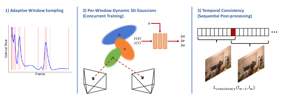
Figure 2: Method overview. First, we adaptively partition a dynamic sequence into windows based on 2D optical flow across all views. We sample windows frequently in high-motion areas and less frequently otherwise. Second, we train a separate dynamic 3DGS model for each window. Tunable MLPs model the scene’s dynamic parts by learning deformations from per-window canonical representations. MLPs are conditioned on frequency-encoded positions $\gamma(\boldsymbol{x})$, frame time $\gamma(t)$, and learnable blending parameters $\boldsymbol{\alpha}$, which weighs the MLP’s parameters for each Gaussian respectively, enabling it to focus on dynamic parts. The MLP outputs displacements of each Gaussian’s position $\Delta\boldsymbol{x}$, rotation $\Delta\boldsymbol{r}$, and scale $\Delta\boldsymbol{s}$. Thirdly, we fine-tune each model sequentially to enforce inter-window temporal consistency. Neighbouring windows share overlapping frames, on which we apply consistency loss on randomly sampled novel view renders.

Overview

We present our method to reconstruct and render novel views of general dynamic scenes from multiple time-synchronized and calibrated cameras. An overview of our method is shown in Fig. 2. Our method is built upon 3D Gaussian Splatting [15] for novel view synthesis of static scenes, which we extend to scenes containing motion.

Our method can be separated into three main steps. First, given a dynamic sequence of arbitrary length, we split the sequence into separate shorter windows of frames for concurrent processing. We adaptively sample windows of varying lengths depending on the amount of motion within the sequence. Each sampled window contains a single overlapping frame between adjacent windows to enable temporal consistency to be enforced over the sequence at a subsequent training stage. Partitioning the sequence into smaller windows enables us to deal with sequences of any length while maintaining a high level of render quality.

Second, we train separate dynamic 3DGS models for each window in turn. We extend the static 3DGS method to model the dynamics within each window by introducing a tuneable MLP [27]. The MLP learns the deformation field from a canonical set of 3D Gaussians to each frame in a window. We learn independent Gaussian models for each window, comprising a per-window canonical representation and deformation field. All 3D Gaussian parameters are allowed to change between windows, including the number of Gaussians, their positions, rotations, scaling, colours and opacities. This enables us to process scenes of any frame length, handle significant geometric or topological changes, and/or if new objects appear throughout the sequence, which can be challenging to model with a single canonical representation. Furthermore, independent models can be trained in parallel across multiple GPUs to speed up training. A tuneable MLP weighting parameter is learned for each 3D Gaussian to enable the MLP to focus on modelling the dynamic parts of the scene, with the static parts encapsulated by the canonical representation.

Third, once a dynamic 3DGS model is trained for each window in the sequence, we apply a post-process fine-tuning step to enforce temporal consistency throughout the sequence. We fine-tune each Gaussian Splatting model sequentially and employ a self-supervising temporal consistency loss on the overlapping frame renders between neighbouring windows. This encourages the model of the current window to produce similar renderings to the previous window. At this fine-tuning stage, we fix the MLP weights and allow only the canonical representations to change. The result is a set of per-frame Gaussian Splatting models enabling high-quality novel view renderings of dynamic scenes with real-time interactive viewing capability. Our approach enables us to overcome the limitations of training with long sequences and to handle complex motions without exhibiting distracting temporal flickering.

In summary, the main contributions of our method are:

1. An adaptive window sampling approach that enables the reconstruction of arbitrary length sequences whilst maintaining high rendering quality.

2. An MLP mechanism to model dynamic scenes by learning a deformation field from canonical to each frame in a window, unique to each sampled window.

3. A learnable MLP tuning parameter to focus the MLP on the dynamic parts of the scene, thereby disentangling the 3D Gaussians into static canonical and dynamic parts.

4. A post-process fine-tuning stage to ensure temporal consistency over the sequence.

3.1 Preliminary: 3D Gaussian Splatting

Our method is built on the 3D Gaussian Splatting [15] framework. 3DGS uses a 3D Gaussian representation to model static scenes as they are differentiable and can be easily projected to 2D splats, allowing fast $\alpha$-blending for image rendering. The 3D Gaussians are defined by 3D covariance matrix $\Sigma$ in world space centered at the mean $\mu$:

$$G(x)=e^{-\frac{1}{2}(x)^{T}\Sigma^{-1}(x)}$$ (1)

To project 3D Gaussians to 2D for rendering, given a viewing transformation $W$, the covariance matrix $\Sigma^{\prime}$ in camera coordinates is given as follows:

$$\Sigma^{\prime}=JW\Sigma W^{T}J^{T}$$ (2)

where $J$ is the Jacobian of the affine approximation of the projective transformation. Given a scaling matrix $S$ and rotation matrix $R$, the corresponding covariance matrix $\Sigma$ of a 3D Gaussian can be written as:

$$\Sigma=RSS^{T}R^{T}$$ (3)

To represent the scene, 3DGS creates a dense set of 3D Gaussians and optimizes for their positions $\boldsymbol{x}$, covariance $\Sigma$ and $\alpha$, in addition to their colours, represented by spherical harmonic (SH) coefficients, to capture the view-dependent appearance. Optimization of these parameters is interleaved with steps controlling Gaussian density. The model is optimized by rendering the learned Gaussians via a differentiable rasterizer, comparing the resulting image $I_{r}$ against the ground truth $I_{gt}$, and minimizing the loss function:

$$\mathcal{L}=(1-\lambda)\mathcal{L}_{1}(I_{r},I_{gt})+\lambda\mathcal{L}_{\mathrm{SSIM}}(I_{r},I_{gt}).$$ (4)

3.2 Adaptive Window Sampling

Using a single dynamic Gaussian Splatting model for an entire sequence becomes impractical for longer sequences, simply from a data processing standpoint. Furthermore, representing an extended sequence with a single dynamic model performs significantly worse than using multiple fixed-sized segments, particularly if the scene has significant motion or large geometric or topological changes that can’t be represented easily with just one canonical representation and deformation field. Therefore, given an input dynamic sequence, we separate the sequence into smaller windows of frames by adaptively sampling windows of different lengths, depending on the amount of motion exhibited in the sequence. In areas of high motion, we sample windows more frequently (shorter windows), and in areas of low motion, we sample less frequently (longer windows).

We follow a similar approach to that of Işık et al. [13], who partition the sequence based on temporal changes in per-frame occupancy grids. In our case, we don’t use occupancy grids but rather the magnitude of 2D optical flow in each camera viewpoint. We employ a greedy algorithm to adaptively select the sizes of windows before training based on the mean optical flow magnitudes. Specifically, we estimate the per-frame optical flow $\boldsymbol{f}$ using a pre-trained RAFT [41] model for each camera view $j\in Views$ and all frames in the sequence $i\in N$, and compute the mean flow magnitude for each image frame:

$$\hat{v}_{i}=\frac{1}{Views}\sum^{Views}_{j}\frac{1}{N-1}\sum^{N-1}_{i}||\boldsymbol{f}(I^{j}_{i},I^{j}_{i+1})||^{2}_{2}$$ (5)

We iterate over each frame in the sequence with a greedy heuristic and generate a new window when the mean flow magnitude over all camera views $\hat{v}_{i}$ exceeds a certain pre-defined threshold. This ensures that each window represents a similar amount of movement, leading to a balanced distribution of the total model representation workload.

We note that each sampled window overlaps with the subsequent window by a single frame, so adjacent windows share a common image frame. This is to enable cross-window temporal consistency, as discussed in section 3.5.

3.3 Dynamic 3D Gaussians

To extend static 3D Gaussian Splatting to handle dynamic scenes, we introduce a dynamic and tunable MLP representation, unique to each sampled window in the sequence. Each time-dependent MLP learns a deformation field for the set of 3D Gaussians, mapping from a learned per-window canonical space to a set of 3D Gaussians for each frame in the window. Each deformation field, represented by a small MLP $\mathcal{F}_{\theta}$ with weights $\theta$, takes as input the normalized frame time $t\in[0,1]$ and the locations of the 3D Gaussian means $\boldsymbol{x}$, and outputs the displacements to their positions $\Delta\boldsymbol{x}$, rotations $\Delta\boldsymbol{r}$ and scaling $\Delta\boldsymbol{s}$:

$$\Delta\boldsymbol{x},\Delta\boldsymbol{r},\Delta\boldsymbol{s}=\mathcal{F}_{\theta}(\gamma({\boldsymbol{x}}),\gamma(t))$$ (6)

where $\gamma(.)$ denotes sinusoidal positional encoding $\gamma:\mathbb{R}^{3}\rightarrow\mathbb{R}^{3+6m}$:

$$\gamma(x)=(x,\dots,\sin(2k\pi x),\cos(2k\pi x),\dots)$$ (7)

We set the number of frequency components $m=6$, MLP depth $D=4$, width $W=16$, with two skip connections.

3.4 Tunable Dynamic MLPs

Ideally, the time-dependent MLP representation should model motion in the scene by associating the dynamic parts with the temporal input component $\gamma(t)$ and thus learn to decouple the scene into static canonical and dynamic 3D Gaussians. However, in scenes with a large imbalance of static vs dynamic parts, e.g. scenes with a static background such as the Neural 3D Video dataset [19], the MLP struggles to disentangle dynamic and static regions, resulting in a poorly estimated deformation field. This is likely because the MLP is overwhelmed with mostly static inputs.

To counteract this, we introduce tuneable dynamic MLPs [27] (i.e. MLPs with several sets of weights) governed by a learnable blending parameter $\boldsymbol{\alpha}=\{\alpha_{i}\}^{N}_{i=0}$ for each 3D Gaussian $i\in N$. The tuning parameter weighs the respective parameters of the MLP to focus its attention on the dynamic parts of the scene, thus decoupling the static and dynamic Gaussians in a smoothly weighted manner. Given blending parameter $\alpha_{i}$ for the $i$-th input Gaussian $\boldsymbol{x}$, the output from the MLP $y_{i}$ can be written as:

$$y_{i}=\phi\left(\alpha_{i}\sum^{K}_{k=1}w_{k}x_{k}+\alpha_{i}b\right)=\phi\left(\alpha_{i}(\boldsymbol{w}^{T}\boldsymbol{x}+b)\right)$$ (8)

We implement the dynamic MLP as a single batch matrix multiplication in PyTorch. We initialize blending parameters $\boldsymbol{\alpha}$ with an initial binary mask estimate of the dynamic Gaussians, where 0 defines a static Gaussian, and 1 is dynamic. For a given window, we project all the 3D Gaussian positions into each camera view: $u=\Pi_{j}({\boldsymbol{x}})$ to obtain their 2D-pixel coordinates. We compute the L1 image differences from the central frame to each frame in the window, providing a rough estimate of which pixels belong to the dynamic parts. For each projected 2D location, if the absolute pixel difference is larger than a certain threshold, we label that Gaussian 1 (dynamic); otherwise, it is labelled 0 (static). To account for occlusions and mislabelling, we compute the average assigned label over all views and frames, and if the average is greater than 0.5, we label the Gaussian as dynamic, otherwise static.

Once initialized, we allow soft-weighting parameter $\boldsymbol{\alpha}$ to optimize during training. We assume $\boldsymbol{\alpha}$ is constant for all frames in a window to reduce the complexity of the optimization, which is a fair assumption given our adaptive window sampling mechanism. Fig. 3 visualizes the effect of learning the MLP tuning parameter. We observe $\boldsymbol{\alpha}$ providing higher weight to Gaussians more likely to be dynamic. Fig. 3 (right) plots the magnitudes of resulting displacements $\Delta\boldsymbol{x}$ output by the MLP. Note that the soft-weighting parameter does not necessarily have to be entirely accurate, as the MLP can learn to adjust accordingly, yet it enables the MLP to better deal with highly imbalanced scenes.

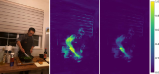
Figure 3: To deal with scenes exhibiting an imbalance in static and dynamic regions, we learn a dynamic MLP with tunable parameter $\boldsymbol{\alpha}$ for each Gaussian, which weighs the parameters of the MLP for each input. For visualization purposes, we render the following: left: predicted image render, middle: tunable $\boldsymbol{\alpha}$ parameters, and right: the normalized output of the MLP displacements $\Delta\boldsymbol{x}$. Note, that the learned $\boldsymbol{\alpha}$ highlights the scene’s mostly dynamic regions.

3.5 Temporal Consistency Fine-tuning

Due to the non-deterministic nature of the 3DGS optimization, models trained independently for each window produce slightly different results. When the resulting renders are played back from each model in sequence, unsightly flickering can be observed, mainly in novel views (the effect is less noticeable in training views). Therefore, once we have trained all adaptively sampled windows in the sequence separately, we address inter-window temporal flickering by introducing a temporal consistency fine-tuning step with a self-supervising loss function to transition between the models of the separate windows smoothly.

We fine-tune each model for a short period (3000 iterations in our experiments), starting from the first window and moving forward sequentially. Given a trained model for a specific window of frames, we also load the 3D Gaussian model from the window directly preceding it, with one overlapping frame between them. During fine-tuning, as the flickering is mainly observed in novel views, we randomly sample novel test views in between the training views by interpolating the training camera poses $P^{4\times 4}_{j}=[R|\boldsymbol{t}]$:

$$P_{\mathrm{novel}}=\exp_{\mathrm{M}}\sum^{Views}_{j}w_{j}\log_{\mathrm{M}}(P_{j})$$ (9)

where $\exp_{\mathrm{M}}$ and $\log_{\mathrm{M}}$ are the matrix exponential and logarithm [1] respectively, and $w_{j}\in[0,1]$ is a uniformly sampled weighting such that $\sum^{Views}_{j}w_{j}=1$.

In one fine-tuning step, we render the overlapping frame from a randomly sampled novel view from both the model of the current window and the model from the previous window. We apply a consistency loss, which is simply the L1 loss on the two image renders from both models:

$$\mathcal{L}_{\mathrm{consistency}}=|I_{w}-I_{w-1}|_{1}$$ (10)

As the canonical set of 3D Gaussians is shared for all frames in a window, when fine-tuning the overlapping frame, we must take care not to affect the other frames in the window negatively. Therefore, we fine-tune with an alternating strategy, which alternates between enforcing temporal consistency on the overlapping frame, and training with the remaining training views and frames as usual.

3.6 Implementation Details

We implement our method in PyTorch, building upon the codebase and differentiable rasterizer of 3DGS [15]. We initialize each model with a point cloud obtained from COLMAP [37]. Each dynamic 3DGS model is trained for 15K iterations for all sampled windows in a sequence. The initial 2K iterations comprise a warm-up stage; training with only the central window frame and freezing the weights of the MLP, allowing the canonical representation to stabilize. We optimize the Gaussians’ positions, rotations, scaling, opacities and SH coefficients. Afterwards, we unfreeze the MLP and allow the deformation field and tuning parameters $\boldsymbol{\alpha}$ to optimize. We find this staggered optimization approach leads to better convergence. The number of Gaussians densifies for 8K iterations, after which the number of Gaussians is fixed. Inputs to the MLP are normalized by the mean and standard deviation of the canonical point cloud post-warm-up stage before frequency encoding, leading to faster and stabler convergence. We train with Adam optimizer, using different learning rates for each parameter following the implementation of [15]. The learning rate for the MLP and $\boldsymbol{\alpha}$ parameters are set to 1e-4, with the MLP learning rate undergoing exponential decay by factor 1e-2 in 20K iterations. During the initial optimization phase, due to the independence of each Gaussian model, we train each model in parallel on eight 32Gb Tesla V100 GPUs to speed up training. After, we fine-tune each model sequentially using a single GPU for 3K iterations each.

4 Results

We evaluate our method on the Neural 3D Video dataset [19], comprising real-world dynamic scenes captured using a time-synchronized multi-view capture system at $2028\times 2704$ resolution and a frame rate of 30 FPS. Camera parameters are estimated using COLMAP [37]. We specifically focus on the following scenes: cook spinach, cut roasted beef, flame steak, sear steak. Following previous works, we omit the asynchronously captured coffee martini scene and the lengthy flame salmon scene. We compare our method to several SoTA methods, including K-Planes, Hexplanes, MixVoxels, Hyperreel, NeRFPlayer, and StreamRF. We compute quantitative metrics for the central test view at half the original resolution ($1014\times 1352$) for all 300 frames. The average results for each method over the dataset are given in Table 1, while Table 3 provides a breakdown of the per-scene performance. The results show that our method performs best regarding PSNR and SSIM metrics while offering the fastest rendering performance.

Method	PSNR	SSIM	LPIPS	FPS
MixVoxels	30.94	0.932	0.109	4.30
K-Planes	31.22	0.933	0.109	0.33
Hexplanes	30.58	0.933	0.110	0.24
Hyperreel	31.85	0.937	0.085	3.60
NeRFPlayer	30.25	0.924	0.121	0.10
StreamRF	31.15	0.920	0.154	9.40
Ours	32.05	0.949	0.093	71.51

Table 1: Quantitative results on the Neural 3D Video dataset [19], averaged over scenes: cook spinach, cut roasted beef, flame steak, and sear steak. Best and second best results are highlighted. Our method performs best overall whilst enabling real-time interactive viewing. Per-scene breakdown of results are given in Table 3. Inference frame rates (FPS) are also given for reference.

Method	PSNR	SSIM	LPIPS	VQA
w/o temporal consist.	32.01	0.956	0.085	0.666
w/ temporal consist.	32.05	0.949	0.093	0.726
Ground truth	-	-	-	0.763

Table 2: Ablation study highlighting the impact of temporal consistency fine-tuning. Results are averaged over four scenes from the Neural 3D Video dataset [19]. We measure the temporal consistency using SoTA video quality assessment metric FAST-VQA [47], where the quality score is in the range [0,1]. We incur a minor degradation in per-frame performance but significantly improve temporal consistency and overall perceptual video quality.

Scene	Cook Spinach			Cut Roast Beef			Flame Steak			Sear Steak
Method	PSNR	SSIM	LPIPS	PSNR	SSIM	LPIPS	PSNR	SSIM	LPIPS	PSNR	SSIM	LPIPS
MixVoxels	$31.39$	$0.931$	$0.113$	$31.38$	$0.928$	$0.111$	$30.15$	$0.938$	$0.108$	$30.85$	$0.940$	$0.103$
K-Planes	$31.23$	$0.926$	$0.114$	$31.87$	$0.928$	$0.114$	$31.49$	$0.940$	$0.102$	$30.28$	$0.937$	$0.104$
Hexplanes‡	$31.05$	$0.928$	$0.114$	$30.83$	$0.927$	$0.115$	$30.42$	$0.939$	$0.104$	$30.00$	$0.939$	$0.105$
Hyperreel	$31.77$	$0.932$	$0.090$	$32.25$	$0.936$	$0.086$	$31.48$	$0.939$	$0.083$	$31.88$	$0.942$	$0.080$
NeRFPlayer†	$30.58$	$0.929$	$0.113$	$29.35$	$0.908$	$0.144$	$31.93$	$0.950$	$0.088$	$29.13$	$0.908$	$0.138$
StreamRF	$30.89$	$0.914$	$0.162$	$30.75$	$0.917$	$0.154$	$31.37$	$0.923$	$0.152$	$31.60$	$0.925$	$0.147$
Ours	31.96	0.946	0.094	31.84	0.945	0.099	32.18	0.953	0.087	32.21	0.950	0.092

Table 3: Quantitative results on scenes from the Neural 3D Video Synthesis dataset [19], evaluated for all frames on the test view. †As reported in [2], ‡Natively trained in lower resolution, upscaled. The best and the second best results are highlighted respectively. Our method performs competitively in all metrics, usually coming in either first or second place.

(a)

(b)

(c)

(d)

(e)

(f)

(g)

(h)

(i)

(j)

(k)

(l)

(m)

(n)

(o)

(p)

(q)

(r)

(s)

(t)

Figure 4: Qualitative results on the Neural 3D Video dataset [19]. Scenes include, from top to bottom: i) cook spinach, ii) cut roasted beef, iii) flame steak, and iv) sear steak. Methods shown, from left to right, include MixVoxels, K-Planes, Hyperreel, Ours, and the ground truth.

(a)

(b)

(c)

(d)

(e)

(f)

(g)

(h)

(i)

(j)

Figure 5: Close-up qualitative results on the Neural 3D Video Synthesis dataset [19]. From top to bottom, scenes include: i) cook spinach and ii) flame steak. Methods from left to right include MixVoxels, K-Planes, Hyperreel, Ours, and the ground truth.

4.1 Ablation Study

In this section, we provide an ablation study that shows the effectiveness of our self-supervised temporal consistency fine-tuning strategy. As we train independent dynamic models for each window of frames, randomness in the optimization results in flickering artifacts occurring in the final renders when the frame moves from one window to another. To visualize this, Fig. 6 plots the absolute image error between renders of neighbouring frames, with overlapping frames between neighbouring windows outlined in red. Without temporal consistency, we observe a spike in absolute error on overlapping frames, resulting in undesirable flickering artifact. Whereas, after fine-tuning each model sequentially with our self-supervising temporal consistency loss, the image error in overlapping frames is drastically reduced. In table 2, we compute per-frame image metrics and estimate a measure of the temporal consistency using SoTA video quality assessment metric FAST-VQA [47], where the quality score is in the range [0,1]. The table provides results averaged over all scenes from the Neural 3D Video dataset [19]. Although we incur a minor penalty in some per-frame performance metrics (SSIM and LPIPs), we obtain a significantly higher video quality (VQA) score. This indicates a substantial improvement in temporal consistency and overall perceptual video quality, resulting in a much more pleasing rendering.

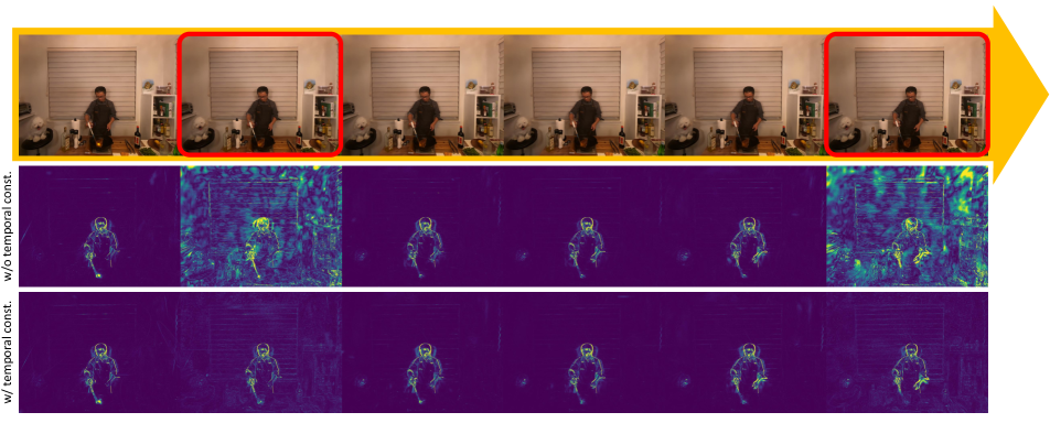
Figure 6: Ablation study on the impact of temporal consistency fine-tuning. We display the absolute error between neighbouring frame renders. Overlapping frames between adjacent windows are highlighted in red. W/o temporal consistency fine-tuning, we observe significant errors between windows. With temporal consistency fine-tuning, the error is substantially reduced. We incur a minor reduction in per-frame performance but significantly improve overall perceptual video quality (VQA) with better temporal consistency and less flickering.

5 Conclusion

We have presented a method to render novel views of dynamic scenes by extending the 3D Gaussian Splatting framework. Results show that our method produces high-quality renderings, even with complex motions like flames. Key to our approach is our adaptive window sampling, which partitions sequences into manageable chunks. Processing each window separately and allowing the canonical representation and deformation field to vary throughout the sequence enables us to handle complex topological changes and/or if new objects enter the scene. In contrast, other methods that learn a single representation for whole sequences are impractical for long sequences and degrade in quality with increasing length. Introducing an MLP for each window lets us learn the deformation field from each canonical representation to a set per-frame 3D Gaussians. Moreover, a learnable tuning parameter helps disentangle static and dynamic parts of the scene, which we find essential for imbalanced scenes. Our ablation shows how self-supervised temporal consistency fine-tuning reduces temporal flickering and improves the overall perceptual video quality, with only a minor impact on per-frame performance metrics. Overall, our method performs strongly compared to recent SoTA and, on average, performs best overall.

References

- Alexa [2002] Marc Alexa. Linear combination of transformations. Proceedings of the 29th annual conference on Computer graphics and interactive techniques, 2002.
- Attal et al. [2023] Benjamin Attal, Jia-Bin Huang, Christian Richardt, Michael Zollhoefer, Johannes Kopf, Matthew O’Toole, and Changil Kim. HyperReel: High-fidelity 6-DoF video with ray-conditioned sampling. In CVPR, 2023.
- Bansal and Zollhoefer [2023] Aayush Bansal and Michael Zollhoefer. Neural Pixel Composition for 3D-4D View Synthesis from Multi-Views. In CVPR, 2023.
- Bansal et al. [2020] Aayush Bansal, Minh Vo, Yaser Sheikh, Deva Ramanan, and Srinivasa Narasimhan. 4D Visualization of Dynamic Events from Unconstrained Multi-View Videos. In CVPR, 2020.
- Barron et al. [2021] Jonathan T. Barron, Ben Mildenhall, Matthew Tancik, Peter Hedman, Ricardo Martin-Brualla, and Pratul P. Srinivasan. Mip-nerf: A multiscale representation for anti-aliasing neural radiance fields. In ICCV, pages 5835–5844, 2021.
- Bârsan et al. [2018] Ioan Andrei Bârsan, Peidong Liu, Marc Pollefeys, and Andreas Geiger. Robust Dense Mapping for Large-Scale Dynamic Environments. In ICRA, 2018.
- Cao and Johnson [2023] Ang Cao and Justin Johnson. HexPlane: A Fast Representation for Dynamic Scenes. In CVPR, 2023.
- Chen et al. [2022] Anpei Chen, Zexiang Xu, Andreas Geiger, Jingyi Yu, and Hao Su. Tensorf: Tensorial radiance fields. In ECCV, 2022.
- Du et al. [2021] Yilun Du, Yinan Zhang, Hong-Xing Yu, Joshua B. Tenenbaum, and Jiajun Wu. Neural radiance flow for 4d view synthesis and video processing. In ICCV, 2021.
- Fang et al. [2022] Jiemin Fang, Taoran Yi, Xinggang Wang, Lingxi Xie, Xiaopeng Zhang, Wenyu Liu, Matthias Nießner, and Qi Tian. Fast Dynamic Radiance Fields with Time-Aware Neural Voxels. In SIGGRAPH Asia 2022 Conference Papers, 2022.
- Fridovich-Keil et al. [2023] Sara Fridovich-Keil, Giacomo Meanti, Frederik Rahbæk Warburg, Benjamin Recht, and Angjoo Kanazawa. K-Planes: Explicit Radiance Fields in Space, Time, and Appearance. In CVPR, 2023.
- Hedman et al. [2021] Peter Hedman, Pratul P. Srinivasan, Ben Mildenhall, Jonathan T. Barron, and Paul Debevec. Baking Neural Radiance Fields for Real-Time View Synthesis. In ICCV, 2021.
- Işık et al. [2023] Mustafa Işık, Martin Rünz, Markos Georgopoulos, Taras Khakhulin, Jonathan Starck, Lourdes Agapito, and Matthias Nießner. Humanrf: High-fidelity neural radiance fields for humans in motion. ACM TOG, 42(4):1–12, 2023.
- Joo et al. [2014] Hanbyul Joo, Hyun Soo Park, and Yaser Sheikh. Map visibility estimation for large-scale dynamic 3d reconstruction. In CVPR, 2014.
- Kerbl et al. [2023] Bernhard Kerbl, Georgios Kopanas, Thomas Leimkühler, and George Drettakis. 3D Gaussian Splatting for Real-Time Radiance Field Rendering. ACM TOG, 42(4), 2023.
- Li et al. [2020] Lingzhi Li, Zhen Shen, Zhongshu Wang, Li Shen, and Ping Tan. D-NeRF: Neural Radiance Fields for Dynamic Scenes. In CVPR, 2020.
- Li et al. [2022a] Lingzhi Li, Zhen Shen, Zhongshu Wang, Li Shen, and Ping Tan. Streaming Radiance Fields for 3D Video Synthesis. In NeurIPS, 2022a.
- Li et al. [2022b] Ruilong Li, Julian Tanke, Minh Vo, Michael Zollhofer, Jurgen Gall, Angjoo Kanazawa, and Christoph Lassner. TAVA: Template-free animatable volumetric actors. In ECCV, 2022b.
- Li et al. [2022c] Tianye Li, Mira Slavcheva, Michael Zollhöfer, Simon Green, Christoph Lassner, Changil Kim, Tanner Schmidt, Steven Lovegrove, Michael Goesele, Richard Newcombe, and Zhaoyang Lv. Neural 3D Video Synthesis from Multi-view Video. In CVPR, 2022c.
- Li et al. [2021] Zhengqi Li, Simon Niklaus, Noah Snavely, and Oliver Wang. Neural Scene Flow Fields for Space-Time View Synthesis of Dynamic Scenes. In CVPR, 2021.
- Li et al. [2023] Zhengqi Li, Qianqian Wang, Forrester Cole, Richard Tucker, and Noah Snavely. DynIBaR: Neural Dynamic Image-Based Rendering. In CVPR, 2023.
- Lin et al. [2021] Kai-En Lin, Lei Xiao, Feng Liu, Guowei Yang, and Ravi Ramamoorthi. Deep 3D Mask Volume for View Synthesis of Dynamic Scenes. In ICCV, 2021.
- Liu et al. [2023] Yu-Lun Liu, Chen Gao, Andreas Meuleman, Hung-Yu Tseng, Ayush Saraf, Changil Kim, Yung-Yu Chuang, Johannes Kopf, and Jia-Bin Huang. Robust Dynamic Radiance Fields. In CVPR, 2023.
- Lombardi et al. [2019] Stephen Lombardi, Tomas Simon, Jason Saragih, Gabriel Schwartz, Andreas Lehrmann, and Yaser Sheikh. Neural Volumes: Learning Dynamic Renderable Volumes from Images. ACM TOG, 38(4), 2019.
- Luiten et al. [2020] Jonathon Luiten, Tobias Fischer, and Bastian Leibe. Track to reconstruct and reconstruct to track. IEEE Robotics and Automation Letters, 5(2):1803–1810, 2020.
- Luiten et al. [2024] Jonathon Luiten, Georgios Kopanas, Bastian Leibe, and Deva Ramanan. Dynamic 3D Gaussians: Tracking by Persistent Dynamic View Synthesis. In 3DV, 2024.
- Maggioni et al. [2023] Matteo Maggioni, Thomas Tanay, Francesca Babiloni, Steven G. McDonagh, and Alevs Leonardis. Tunable convolutions with parametric multi-loss optimization. In CVPR, 2023.
- Mildenhall et al. [2020] Ben Mildenhall, Pratul P. Srinivasan, Matthew Tancik, Jonathan T. Barron, Ravi Ramamoorthi, and Ren Ng. NeRF: Representing Scenes as Neural Radiance Fields for View Synthesis. In ECCV, 2020.
- Müller et al. [2022] Thomas Müller, Alex Evans, Christoph Schied, and Alexander Keller. Instant neural graphics primitives with a multiresolution hash encoding. ACM Trans. Graph., 41(4):102:1–102:15, 2022.
- Newcombe et al. [2015] Richard A. Newcombe, Dieter Fox, and Steven M. Seitz. Dynamicfusion: Reconstruction and tracking of non-rigid scenes in real-time. In CVPR, 2015.
- Niemeyer et al. [2021] Michael Niemeyer, Jonathan T. Barron, Ben Mildenhall, Mehdi S. M. Sajjadi, Andreas Geiger, and Noha Radwan. Regnerf: Regularizing neural radiance fields for view synthesis from sparse inputs. In CVPR, pages 5470–5480, 2021.
- Park et al. [2021a] Keunhong Park, Utkarsh Sinha, Jonathan T. Barron, Sofien Bouaziz, Dan B Goldman, Steven M. Seitz, and Ricardo Martin-Brualla. Nerfies: Deformable Neural Radiance Fields. ICCV, 2021a.
- Park et al. [2021b] Keunhong Park, Utkarsh Sinha, Peter Hedman, Jonathan T. Barron, Sofien Bouaziz, Dan B Goldman, Ricardo Martin-Brualla, and Steven M. Seitz. HyperNeRF: A Higher-Dimensional Representation for Topologically Varying Neural Radiance Fields. ACM TOG, 40(6), 2021b.
- Peng et al. [2021] Sida Peng, Junting Dong, Qianqian Wang, Shangzhan Zhang, Qing Shuai, Xiaowei Zhou, and Hujun Bao. Animatable neural radiance fields for modeling dynamic human bodies. In ICCV, 2021.
- Peng et al. [2023] Sida Peng, Yunzhi Yan, Qing Shuai, Hujun Bao, and Xiaowei Zhou. Representing Volumetric Videos as Dynamic MLP Maps. In CVPR, 2023.
- Reiser et al. [2021] Christian Reiser, Songyou Peng, Yiyi Liao, and Andreas Geiger. KiloNeRF: Speeding up Neural Radiance Fields with Thousands of Tiny MLPs. In ICCV, 2021.
- Schönberger and Frahm [2016] Johannes L. Schönberger and Jan-Michael Frahm. Structure-from-motion revisited. In CVPR, pages 4104–4113, 2016.
- Shao et al. [2023] Ruizhi Shao, Zerong Zheng, Hanzhang Tu, Boning Liu, Hongwen Zhang, and Yebin Liu. Tensor4D: Efficient Neural 4D Decomposition for High-fidelity Dynamic Reconstruction and Rendering. In CVPR, 2023.
- Slavcheva et al. [2017] Miroslava Slavcheva, Maximilian Baust, Daniel Cremers, and Slobodan Ilic. KillingFusion: Non-rigid 3D Reconstruction without Correspondences. In CVPR, 2017.
- Song et al. [2023] Liangchen Song, Anpei Chen, Zhong Li, Zhang Chen, Lele Chen, Junsong Yuan, Yi Xu, and Andreas Geiger. NeRFPlayer: A Streamable Dynamic Scene Representation with Decomposed Neural Radiance Fields. IEEE Transactions on Visualization and Computer Graphics, 29(5):2732–2742, 2023.
- Teed and Deng [2020] Zachary Teed and Jia Deng. RAFT: Recurrent All-Pairs Field Transforms for Optical Flow. In ECCV, 2020.
- Turki et al. [2023] Haithem Turki, Jason Y Zhang, Francesco Ferroni, and Deva Ramanan. SUDS: Scalable Urban Dynamic Scenes. In CVPR, 2023.
- Wang et al. [2023] Feng Wang, Sinan Tan, Xinghang Li, Zeyue Tian, and Huaping Liu. Mixed Neural Voxels for Fast Multi-view Video Synthesis. In ICCV, 2023.
- Wang et al. [2022] Liao Wang, Jiakai Zhang, Xinhang Liu, Fuqiang Zhao, Yanshun Zhang, Yingliang Zhang, Minye Wu, Jingyi Yu, and Lan Xu. Fourier plenoctrees for dynamic radiance field rendering in real-time. In CVPR, 2022.
- Wang et al. [2021] Qianqian Wang, Zhicheng Wang, Kyle Genova, Pratul Srinivasan, Howard Zhou, Jonathan T. Barron, Ricardo Martin-Brualla, Noah Snavely, and Thomas Funkhouser. IBRNet: Learning Multi-View Image-Based Rendering. In CVPR, 2021.
- Weng et al. [2022] Chung-Yi Weng, Brian Curless, Pratul P. Srinivasan, Jonathan T. Barron, and Ira Kemelmacher-Shlizerman. HumanNeRF: Free-Viewpoint Rendering of Moving People From Monocular Video. In CVPR, 2022.
- Wu et al. [2022] Haoning Wu, Chaofeng Chen, Jingwen Hou, Liang Liao, Annan Wang, Wenxiu Sun, Qiong Yan, and Weisi Lin. Fast-vqa: Efficient end-to-end video quality assessment with fragment sampling. In ECCV, 2022.
- Xian et al. [2021] Wenqi Xian, Jia-Bin Huang, Johannes Kopf, and Changil Kim. Space-time Neural Irradiance Fields for Free-Viewpoint Video. In CVPR, 2021.
- Xing and Chen [2022] Wenpeng Xing and Jie Chen. Temporal-MPI: Enabling Multi-Plane Images For Dynamic Scene Modelling Via Temporal Basis Learning. In ECCV, page 323–338, 2022.
- Yu et al. [2021] Alex Yu, Ruilong Li, Matthew Tancik, Hao Li, Ren Ng, and Angjoo Kanazawa. PlenOctrees for real-time rendering of neural radiance fields. In ICCV, 2021.
- Zhao et al. [2022] Fuqiang Zhao, Wei Yang, Jiakai Zhang, Pei Lin, Yingliang Zhang, Jingyi Yu, and Lan Xu. Humannerf: Efficiently generated human radiance field from sparse inputs. In CVPR, pages 7743–7753, 2022.
- Zhou et al. [2018] Tinghui Zhou, Richard Tucker, John Flynn, Graham Fyffe, and Noah Snavely. Stereo magnification: Learning view synthesis using multiplane images. ACM TOG, 37, 2018.