Not All Steps are Equal: Efficient Generation with Progressive Diffusion Models

Abstract

Diffusion models have demonstrated remarkable efficacy in various generative tasks with the predictive prowess of denoising model. Currently, these models employ a uniform denoising approach across all timesteps. However, the inherent variations in noisy latents at each timestep lead to conflicts during training, constraining the potential of diffusion models. To address this challenge, we propose a novel two-stage training strategy termed Step-Adaptive Training. In the initial stage, a base denoising model is trained to encompass all timesteps. Subsequently, we partition the timesteps into distinct groups, fine-tuning the model within each group to achieve specialized denoising capabilities. Recognizing that the difficulties of predicting noise at different timesteps vary, we introduce a diverse model size requirement. We dynamically adjust the model size for each timestep by estimating task difficulty based on its signal-to-noise ratio before fine-tuning. This adjustment is facilitated by a proxy-based structural importance assessment mechanism, enabling precise and efficient pruning of the base denoising model. Our experiments validate the effectiveness of the proposed training strategy, demonstrating an improvement in the FID score on CIFAR10 by over 0.3 while utilizing only 80% of the computational resources. This innovative approach not only enhances model performance but also significantly reduces computational costs, opening new avenues for the development and application of diffusion models.

1 Introduction

Generative models, exemplified by pioneering approaches such as generative adversarial networks (GANs) [6, 3, 39, 25], flows [40], autoregressive models [13], and variational autoencoders (VAEs) [14], have showcased profound capabilities across diverse applications. Among these, diffusion models [10] represent the forefront of generative modeling, achieving notable success in areas like image generation [36, 28, 37, 35, 38, 30, 1], super-resolution [32], and video synthesis [11, 41]. Inherent to diffusion models is their utilization of thousands of timesteps, employing a unified denoising model to predict noise across different levels and temporal instances. However, the substantial variations in noise magnitudes at each timestep present a formidable challenge. The attempt to have a single denoising model cover all noise distributions hampers efficiency, leading to slower convergence, increased training overhead, and compromised performance [9].

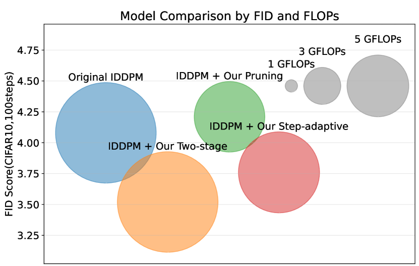
Figure 1: Visualization of Diffusion Model Performance: Circle sizes represent computational costs (GFLOPs) while vertical positioning indicates FID scores.

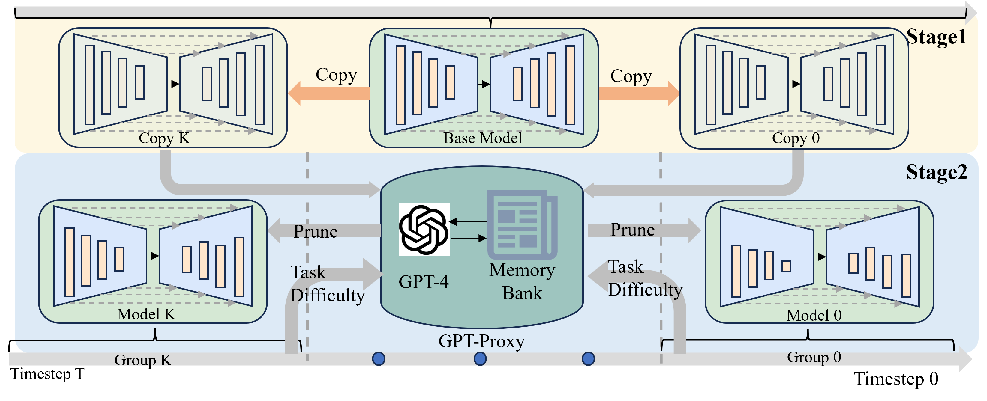
Figure 2: Pipeline of Our Training Strategy. In the first stage, we train a base denoising model across all timesteps, subsequently duplicating it for each group of timesteps. During the second stage, we employ GPT-Proxy Pruning to prune the copies of the base model. This is followed by fine-tuning on the intra-group timesteps to achieve a more specialized model.

To address this issue, a straightforward approach is to decouple the noise prediction by learning distinct denoising models for each timestep. However, this seemingly intuitive solution introduces a significant drawback – training thousands of models becomes impractical, incurring prohibitively high costs and potentially diminishing synergy between timesteps. Recognizing that adjacent timesteps share similar data distributions and signal-to-noise ratios, we advocate for a more efficient and effective strategy. Rather than training individual models for each timestep, we propose a continuous partitioning of timesteps into multiple groups, assigning an independent denoising model to each group. This approach leverages the inherent similarity between adjacent timesteps, mitigating optimization conflicts and potentially enhancing performance through richer training samples at mutually-cooperated timesteps. To manage the training cost associated with multiple denoising models, we introduce a two-stage training strategy. Initially, a basic and general model is trained across all timesteps. Subsequently, this model is distributed and fine-tuned independently on each timestep group. This two-stage divide-and-conquer strategy effectively alleviates conflicts between distinct timesteps, introducing only marginal additional training cost.

The variability across different timesteps extends beyond distinct prediction objectives; it also encompasses variations in learning difficulty. Consider two noisy latents—one with minor noise, revealing clear original image content, and another with substantial noise, containing limited original information. It becomes evident that the denoising model can more easily adapt to the former. In pursuit of a more efficient diffusion model, we advocate for a dynamic allocation of computation resources based on the difficulty inherent to each timestep. This difficulty is intricately tied to the signal-to-noise ratio characterizing each timestep. Consequently, we propose a strategy that dynamically assigns more computation resources to models operating within challenging timesteps. This allocation is tailored to the specific difficulty posed by the signal-to-noise ratio at each timestep, enhancing the overall efficiency of the diffusion model.

To achieve the adjustment of model, we propose a structural pruning method to slim the redundant weights in the model and decrease its computation cost to a certain value computed by our dynamic allocation. Diverging from common pruning methods that rely on magnitude-based assessment [17], loss variation sensitivity [20], and other metrics, which may not align seamlessly with diffusion models due to the sensitivity of model outputs to even minor alterations, we advocate for a more effective and precise importance evaluation mechanism. This mechanism is crucial for accurate pruning to maintain the model’s performance to the utmost degree. Our proposed approach leverages the capabilities of GPT-4 [24], a cutting-edge large-scale general-purpose language model renowned for its formidable prowess in data analysis and the design of complex algorithms [2]. We treat the importance evaluation in pruning as a iterative decision task in GPT-4, allowing it to select redundant parameters that require pruning. This process is enhanced by continuous feedback on model performance to enrich the knowledge base.

In conclusion, our method, a combination of a two-stage divide-and-conquer strategy to derive multiple independent denoising models and a dynamic computation resource allocation method that prunes each model to align with their learning difficulties, attains superior performance and efficiency. Our contributions are summarized as follows:

1. We introduce a Step-Adaptive Training Framework for diffusion models, addressing the timestep conflicts inherent in diffusion models. This framework accelerates the training with progressive diffusion models.

2. We propose a two-stage training strategy, coupled with a proxy-based diffusion model pruning algorithm, to customize models of varying scales and capabilities according to the task difficulty and characteristics of different temporal steps.

3. Compared to the original IDDPM, the incorporation of our Step-Adaptive Training Strategy has improved the FID on CIFAR-10 and ImageNet64 by 0.32 and 1.5, respectively, and reduced computational requirements by approximately 20%.

2 Related Work

2.1 Network Pruning

Model Pruning, a method to optimize deep learning models, involves removing parameters to reduce size and complexity while preserving accuracy. It is mainly utilized for efficient deployment on edge devices, conserving resources and energy [8, 26]. Pruning is classified into unstructured and structured types. Unstructured pruning eliminates individual weights, resulting in sparse matrices that need specific hardware or software for efficiency [15]. Structured pruning, however, removes entire neurons or kernels, directly reducing layer dimensions and is more compatible with conventional hardware [18, 22].

A central issue during the pruning process is how to assess the “importance” of each parameter within the network. Some studies use the magnitude of the weights as a criterion, positing that weights with smaller absolute values have a lesser impact on the model and can therefore be pruned [7]. Another approach is gradient-based, determining importance by examining the sensitivity of the model’s output to the weights [34]. There are also proposals that advocate for pruning based on changes in model output, which typically involves setting a tolerance for the acceptable degradation in model performance post-pruning [27].

2.2 Improvement of Diffusion Models

Advancements in diffusion models mainly focus on sampling efficiency and sample fidelity. For efficiency, one approach eliminates the Markov chain of DDPM to reduce sampling steps [23, 42], while another employs knowledge distillation to condense the multi-step denoising of a ’teacher’ model into a single step in a ’student’ model [33, 12]. In terms of sample quality, strategies include introducing learnable variance in models like Improved Denoising Diffusion Probabilistic Models (IDDPM) to enhance distribution fitting [29]. Another tactic is refining the optimization objective, aligning it closer to the model’s real objective, the log likelihood, to address the variational discrepancy present in traditional approaches.

3 Revisiting Diffusion Models

Diffusion probability model[10] is a kind of latent variable model, with the workflow composed of a forward diffusion process and a reverse denoising process.

3.1 Forward Process

The original data distribution can be defined as $q(\mathbf{x}_{0})$. In the forward diffusion process, given an original data $\mathbf{x}_{0}\sim q(\mathbf{x}_{0})$, a total of $T$ diffusion steps are undertaken, getting $T$ noisy latent variables,$\mathbf{x}_{1},\mathbf{x}_{2},\mathbf{x}_{3}...\mathbf{x}_{T}$, each possessing the same dimension as $\mathbf{x}_{0}$. The diffusion step $t$ is achieved by adding Gaussian noise to $\mathbf{x}_{t-1}$:

$$q(\mathbf{x}_{t}|\mathbf{x}_{t-1}):=\mathcal{N}(\mathbf{x}_{t};\sqrt{1-\beta_{t}}\mathbf{x}_{t-1},\beta_{t}\mathbf{I}),$$ (1)

where $\beta_{t}$ is a small positive constant between 0 and 1, representing the variance of each diffusion step.

3.2 Reverse Denoising Process

It can be easily observed that when $T$ is large enough, the final $\mathbf{x}_{T}$ completely transforms from the original data into random Gaussian noise. Consequently, in the reverse denoising process, an $\mathbf{x}_{T}\sim\mathcal{N}(0,1)$ is sampled from the standard Gaussian distribution as the initial noise. If a neural network can fit the reverse process of the forward diffusion, this random noise $\mathbf{x}_{T}$ can be transformed into a target sample. The reverse distribution from $\mathbf{x}_{t}$ to $\mathbf{x}_{t-1}$ is defined as follows:

$$p_{\theta}(\mathbf{x}_{t-1}|\mathbf{x}_{t}):=\mathcal{N}(\mathbf{x}_{t-1};\mu_{\theta}(\mathbf{x}_{t},t),\sigma_{t}^{2}\mathbf{I}),$$ (2)

where $\mu_{\theta}(x_{t},t)$ is the mean of reverse distribution obtained from a neural network, and $\sigma_{t}$ is the variance of the reverse distribution obtained from $\beta_{t}$:

$$\sigma_{t}=\sqrt{1-(\prod_{i=1}^{t}\sqrt{1-\beta_{i}})^{2}}.$$ (3)

3.3 Training and Sampling

In the practical application of diffusion models, researchers use denoising autoencoders to directly predict the noise that needs to be eliminated at each step, which yields better results than predicting the mean of distribution. In the $k$-th iteration of training, parameters of denoising autoencoder are updated as follows:

$$\theta_{k}=\theta_{k-1}-\lambda\nabla_{\theta}||\mathbf{\epsilon}-\mathcal{U}_{\theta}(\sqrt{\overline{\alpha}_{t}}\mathbf{x}_{0}+\sqrt{1-\overline{\alpha}_{t}}\mathbf{\epsilon},t)||^{2},$$ (4)

where $\alpha_{t}=1-\beta_{t}$, $\overline{\alpha}_{t}=\prod_{i=1}^{t}\alpha_{i}$, $\lambda$ is the learning rate, $\theta$ represents parameters of denoising autoencoder $\mathcal{U}$, $t$ is the diffusion step and $\mathbf{\epsilon}$ is a random noise sampled from Standard Gaussian Distribution $\mathcal{N}(0,1)$.

Once we have a well-trained denoising autoencoder, we can use it to gradually transform the noise $\mathbf{x}_{T}$ into the sample $\mathbf{x}_{0}$.

$$\mathbf{x}_{t-1}=\frac{1}{\sqrt{\alpha_{t}}}\left(\mathbf{x}_{t}-\frac{1-\alpha_{t}}{\sqrt{1-\overline{\alpha}_{t}}}\mathcal{U}_{\theta}(\mathbf{x}_{t},t)\right)+\sigma_{t}\mathbf{\epsilon}.$$ (5)

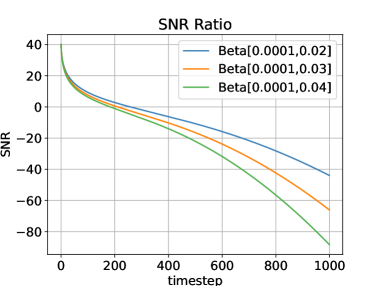
Figure 3: SNR of linear noise schedule

4 Method

In this section, we provide a detailed exposition of our proposed training strategy. In the first subsection, we discuss the inherent differences between various timesteps in diffusion models and analyze how to select suitable model scale based on the level of difficulty. Subsequently, in the second subsection, we introduce the workflow of our two-stage divide-and-conquer diffusion training strategy. Lastly, in the third subsection, we elucidate our dynamic computation resource allocation method, which leverages GPT-4 as a pruning proxy to achieve precise model allocation.

4.1 Unequal Timesteps in Denoising Capacity

Owing to the unique design of our method, where we segregate training across different timesteps and allocate denoising models of varying capacities to different steps, it becomes imperative for us to first investigate the fundamental differences in the tasks undertaken by the denoising model across these timesteps. As indicated by Eq. 5, the denoising task of the model at the $t$ timestep can be modeled as $\mathcal{U}_{\theta}(\mathbf{x}_{t},t)$, highlighting that the variation in tasks across timesteps primarily stems from the distribution differences in $\mathbf{x}_{t}$.

From Eq. 1, the distribution of $\mathbf{x}_{t}$ can be expressed as:

$$\mathbf{x}_{t}=\sqrt{\overline{\alpha}_{t}}\mathbf{x}_{0}+\sqrt{1-\overline{\alpha}_{t}}\mathbf{\epsilon}.$$ (6)

Thus, the distribution of $\mathbf{x}_{t}$ can be regarded as a linear combination of the primary signal $\mathbf{x}_{0}$ and random noise $\mathbf{\epsilon}$. Considering the preceding parameter as the amplitude of the signal, we can compute its Signal-to-Noise Ratio (SNR).

$$SNR=10\log_{10}\left(\frac{\overline{\alpha}_{t}}{1-\overline{\alpha}_{t}}\right).$$ (7)

Taking the linear noise schedule as an example with a diffusion step of 1000, Fig. 3 displays the SNR trends under three different configurations. It’s evident that the task differences across time steps mainly arise from variations in SNR and the distribution of input variables. Adjacent time steps have similar input distributions and SNRs, rendering their tasks quite comparable. It’s observable that tasks across various timesteps possess a strong coherence, and changes occur progressively.

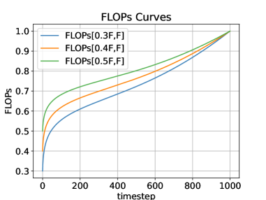
Figure 4: FLOPs of Denoising Models for Different Timesteps

After recognizing that the fundamental differences between different time steps lie in the disparities in distribution and the signal-to-noise ratio (SNR), we can leverage the SNR to evaluate task difficulty, subsequently allocating models of varying sizes to different time steps. When the time step is larger, the SNR is lower, indicating a more challenging task. Thus, a more extensive model should be employed for modeling. Assuming the minimum FLOPs of the model for various time steps is $k\mathcal{F}$, and the maximum is $\mathcal{F}$, the FLOPs of models for different time steps can be determined by normalizing negative SNR values and then mapping them to the range $[k\mathcal{F},\mathcal{F}]$.

$$SNR_{n}=\frac{-SNR-mean(-SNR)}{std(-SNR)}$$ (8)

$$Ratio=\frac{SNR_{n}-min(SNR_{n})}{max(SNR_{n})-min(SNR_{n})}$$

$$FLOPs=(k+(1-k)\times Ratio)\times\mathcal{F}$$

Three examples of FLOPs curves are illustrated in Fig. 4.

4.2 Progressive FLOPs Allocation with Grouped Steps

From the previous analysis of the differences between various timesteps in the diffusion model, it is evident that each timestep requires a different level of model capacity and scale. However, the cost of dedicating a separate model for each timestep and training it from scratch is clearly prohibitive. Fig. 3 and Fig. 4 demonstrate that as timesteps increase, the complexity of the denoising task grows in a monotonic and gradual manner, with adjacent timesteps sharing similar characteristics and levels of difficulty. Thus, a logical approach is to partition all timesteps into $\mathcal{N}$ groups based on the difficulty of the task, with each group sharing a common denoising model. Given that the range of FLOPs across all timesteps is $[k\mathcal{F},\mathcal{F}]$, setting equal intervals for FLOPs between each group, the FLOPs upper limits for each group would be as follows:

$$FLOPs_{g}(i)=(\frac{i}{\mathcal{N}}+\frac{\mathcal{N}-i}{\mathcal{N}}\times k)\mathcal{F},\quad 0\leq i<N.$$ (9)

After determining the upper FLOP limits for each group, we can allocate timesteps into N distinct groups.

$$\mathcal{T}(i)=\{t|v(i)<FLOPs(t)\leq w(i)\},\quad 0\leq i<N$$ (10)

$$v(0)=0,v(i)=FLOPs_{g}(i-1),\quad 0<i<N$$

$$w(i)=FLOPs_{g}(i),\quad 0\leq i<N,$$

where $v(i)$ and $w(i)$ represent the lower and upper FLOPs limits for the $i^{th}$ group, respectively, and $\mathcal{T}(i)$ denotes the set of timesteps included in the $i^{th}$ group. In this way, we also name our obtained models as progressive diffusion models since they are allocated with progressive and grouped FLOPs over timesteps.

4.3 Training for Progressive Diffusion Models

While we have partitioned the timesteps into $\mathcal{N}$ groups, reducing the number of models from $\mathcal{T}$ to $\mathcal{N}$, it remains impractical to design separate models meeting FLOPs constraints for each group and train them from scratch. Therefore, we propose our two-stage Step-Adaptive training strategy for diffusion models.

Two-stage Step-Adaptive Training. In the first stage, we start by training a large-scale base denoising model across all timesteps.

$$\mathcal{U}_{base}^{*}=\mathop{\arg\min}_{\theta}~{}\mathop{Loss}(\mathcal{U}_{base}(\mathcal{T},\mathcal{D},\mathcal{S}))$$ (11)

After acquiring the base denoising model, denoted as $\mathcal{U}_{base}$, in the second stage, we commence by pruning the base model. This process is aimed at deriving the optimal sub-model for each group that conforms to the predefined FLOPs constraint. If we consider the importance evaluation mechanisms as a proxy, this process can be described as follows:

$$\mathcal{U}(i)=\mathcal{U}_{base}^{*}-\theta^{\prime}(i),0\leq i<N$$ (12)

$$\theta^{\prime}(i)=Proxy(\theta,\mathcal{T}(i),\mathcal{D},\mathcal{S},\mathcal{M},FLOPs_{g}(i)),$$

where $\theta^{\prime}(i)$ denotes the structured parameters to be pruned within the $i^{th}$ group, while $\mathcal{U}(i)$ represents the optimal subnetwork obtained for the $i^{th}$ group.

Due to the architectural changes resulting from pruning, it is necessary to fine-tune each model on the timesteps within the group following the pruning to achieve optimal performance.

$$\mathcal{U}^{*}(i)=\mathop{\arg\min}_{\theta}~{}\mathop{Loss}(\mathcal{U}(i))(\mathcal{T}(i),\mathcal{D},\mathcal{S})).$$ (13)

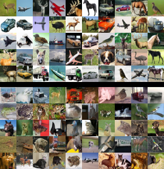
Figure 5: Sample images of IDDPM with (top) and without (bottom) our Step-adaptive training strategy

Proxy-based Pruning. To appropriately allocate model sizes for different groups, we prune the base model before initiating the second phase of training. The objective of model pruning is to reduce the number of parameters and inference overhead of the base model by eliminating non-essential parameters or structures while striving to maintain optimal model performance. Given a dataset $\mathcal{D}$, a base denoising model $\mathcal{U}$, target timesteps $\mathcal{T}$, other settings $\mathcal{S}$, and an upper limit of FLOPs denoted as $f$, the pruning procedure for the diffusion model is as follows:

$${\mathcal{U}_{\theta-\theta^{\prime}}}^{*}=\mathop{\arg\min}_{\theta^{\prime}\in\theta}~{}\mathop{Loss}(\mathcal{U}_{\theta-\theta^{\prime}}(\mathcal{T},\mathcal{D},\mathcal{S}))$$ (14)

$$\text{s.t.}\quad\text{FLOPs}(\mathcal{U}_{\theta-\theta^{\prime}})\leq f,$$

where $\theta$ denotes the parameters of the base denoising model, while $\theta^{\prime}$ indicates the parameters to be pruned. The crux of model pruning lies in identifying the parameters that ought to be eliminated. This essentially involves evaluating and ranking the importance of parameters or structures, then pinpointing the least significant set of parameters. Various methods can be used to assess importance, such as based on the magnitude of parameters or their impact on the loss. If we represent the process of determining the least significant parameters through importance evaluation as $\mathcal{P}$, then LABEL:eq9 can be updated as follows:

$$\theta^{\prime}=\mathcal{P}(\theta,\mathcal{T},\mathcal{D},\mathcal{S}),\ \theta^{\prime}\subseteq\theta$$ (15)

$$\text{s.t.}\quad\text{FLOPs}(\mathcal{U}_{\theta-\theta^{\prime}})\leq f.$$

Traditional importance evaluation methods [16, 5] have shown promising performance for pruning tasks across a variety of model types, however, it is empirically found [4] that they may lose their merits in diffusion models. Actually, we also conduct several benchmark approaches in IDDPM model trained on CIFAR10. However, as demonstrated in Tab. 4, these pruning algorithms result in significant accuracy degradation for diffusion models. These observations remind us that an effective proxy to evaluate and determine the to-be-pruned parameters is of much importance, yet still enjoying fast efficiency since we do not want our training of progressive diffusion models to be slow enough.

Inspired by the success of GPT-NAS [19, 43] in neural architecture search, we also turn to GPT-4’s powerful understanding ability over architectures, and leverage it as a proxy for the assessment of model parameter importance, aiding in the identification of the least important group of parameters. Besides, we also introduce a memory bank to store the performance of each pruned model so that it can serve as a feedback prompt and the whole pruning is implemented in an iterative manner for boosted performance, i.e.

$$\theta^{\prime}=GPT(\theta,\mathcal{T},\mathcal{D},\mathcal{S},\mathcal{M}),\ \theta^{\prime}\subseteq\theta$$ (16)

$$\text{s.t.}\quad\text{FLOPs}(\mathcal{U}_{\theta-\theta^{\prime}})\leq f,$$

where $\mathcal{M}$ denotes the memory bank, which archives the pruned parameters from each pruning iteration along with the performance metrics of the model post-pruning. Its update process is as follows:

$$\mathcal{M}_{i+1}=\mathcal{M}_{i}\cup\left(\theta^{\prime}_{i},Loss(\mathcal{U}_{\theta-\theta^{\prime}_{i}}(\mathcal{T},\mathcal{D},\mathcal{S}))\right).$$ (17)

Table 1: Comparative Results on CIFAR10 and Imagenet64

Dataset	Model	FID	FLOPs	Params
CIFAR10	WaveDiff[31]	4.87	6.06G	38.2M
	PNDM[21]	4.10	6.06G	38.2M
	DDPM[10]	4.19	6.06G	38.2M
	IDDPM[29]	4.08	8.14G	52.5M
	IDDPM+ours	3.76	6.56G	48.7M
ImageNet64	IDDPM	20.7	39.3G	121M
	IDDPM+ours	19.2	32.7G	103M

5 Experiments

As shown in Fig. 5, after incorporating our training strategy, the quality of the sampled images has significantly improved, and the distortions are notably reduced. To further validate the effectiveness of our proposed training strategy, we utilized the representative diffusion model IDDPM as the experimental baseline, conducting experiments on commonly used image generation datasets CIFAR10 and Imagenet64. Across all experiments, we adhered to IDDPM’s standard training configuration, which includes 4000 timesteps, a cosine noise schedule, and a hybrid objective.

In terms of model efficiency evaluation, given that one of the primary limitations of diffusion models is inference speed, we opted for FLOPs as our key metric for assessing inference efficiency. For performance evaluation, we employed the FID (Fréchet Inception Distance) metric to gauge the generative quality and diversity of the models. Recognizing that diffusion models in practical scenarios often employ fast sampling algorithms instead of complete sampling, we aligned our experiments with the real-world use of efficient diffusion. To expedite the experimental process, in all our tests, the performance was evaluated using 100-step fast sampling. As our algorithm involves different models at various timesteps, both the parameter count and FLOPs are calculated as average values across these timesteps.

Table 2: FID Scores for Different Training Methods(same model architecture)

Dataset	Normal Training	Two-stage Training
CIFAR10	4.08	3.52
ImageNet64	20.7	17.6

5.1 Experiment on the Effectiveness of Two-Stage Training

Initially, we conducted comparative experiments to isolate and verify the efficacy of our proposed two-stage divide-and-conquer training strategy. Specifically, during the second stage of training, instead of employing model pruning, we retained the structure of the base model and fine-tuned copies of it across different timestep groups. For standard training of IDDPM on CIFAR10, 500k steps are typically required for convergence. In our two-stage training, we utilized the same denoising model structure and other training configurations. Following Eq. 10, we divided the timesteps into 10 groups. For the CIFAR10 dataset, we trained the base model for 250k steps across all timesteps, then created 10 copies of this base model, each allocated to one of the 10 groups, and subsequently fine-tuned each copy for 3k steps on the timesteps within its group. For the ImageNet64 dataset, we trained for 0.8M steps in the first stage and fine-tuned for 30k steps in the second stage. The experimental results are shown in Tab. 2.

The results demonstrated that our two-stage training strategy achieved a FID of 3.52 on CIFAR10 with just 280k total training steps, which is a significant improvement compared to the FID of 4.08 achieved with the original configuration’s 500k training steps. Similarly, on the ImageNet64 dataset, our approach achieved superior performance with only 73% of the training steps. This indicates that diffusion models indeed have varying capability demands at different timesteps, and employing diverse denoising models at various stages can enhance overall performance. Furthermore, the reduction in total training steps highlights training conflicts between different timesteps, suggesting that separating training across steps can mitigate these conflicts and accelerate convergence.

5.2 Ablation Study on FLOPs Estimation Method

As illustrated in LABEL:eq8, we introduced a strategy to estimate task difficulty based on signal-to-noise ratio (SNR) and subsequently set FLOPs limits for denoising models at each timestep. To prove its effectiveness, we compared it with several other FLOPs schedules. In these experiments, the $k$ value in our proposed FLOPs schedule was set to 0.5. Tab. 3 presents the experimental results obtained after applying various FLOPs schedules to our proposed Step-adaptive Training Strategy. In addition to our schedule, three comparative schedules were included: a consistent FLOPs upper limit across all timesteps; a uniformly increasing FLOPs limit over timesteps; and a uniformly decreasing FLOPs limit over timesteps.

In our algorithm, we merely set an upper limit on FLOPs for the models in each group. The actual FLOPs and parameter counts of the models obtained through GPT-based pruning are not fixed, ensuring only that the models derived from each schedule have approximately similar average FLOPs. The results indicated that at similar average FLOPs, our proposed FLOPs schedule outperformed others in performance, validating that this SNR-based FLOPs schedule can accurately assess task difficulty at each timestep and allocate a reasonable model size accordingly.

Table 3: FID Scores for Different FLOPs Schedule on CIFAR10

Schedule	FID	FLOPs	Params
Our Schedule	3.76	6.56G	48.7M
Constant Schedule	3.91	6.79G	49.5M
Uni-increasing Schedule	3.88	6.85G	43.2M
Uni-decreasing Schedule	4.11	6.21G	45.1M

5.3 Experiment on the Effectiveness of Proxy-Pruning

To evaluate the effectiveness of our proposed pruning algorithm, which uses GPT-4 as a proxy for importance assessment in pruning diffusion models, we designed specific comparative experiments targeting this pruning approach. Given the substantial accuracy loss typically incurred after model pruning, it’s crucial to fine-tune the model post-pruning to adapt it to its new structure. Overfitting is a common challenge during the training of diffusion models, hence selecting the appropriate fine-tuning steps is vital for effective pruning. Using the CIFAR10 dataset as an example, Fig. 6 illustrates the performance of three sub-networks obtained through proxy pruning at various fine-tuning stages. It is evident that immediately after pruning, the model suffers significant performance degradation. However, as fine-tuning progresses, the model performance gradually improves and peaks around 25k steps. Further fine-tuning beyond this point leads to overfitting, diminishing the model’s performance.

Table 4: Performance of Different Pruning Method on CIFAR10

Method	Params	FLOPs	FID	Train Steps
Pretrained	52.5M	8.14G	4.08	500K
Scratch Training	38.7M	5.71G	89.1	25K
Scratch Training	38.7M	5.71G	16.8	100K
Scratch Training	38.7M	5.71G	5.09	500K
Random Pruning	40M	6.02G	4.86	25K
Magnitude Pruning[16]	40M	6.29G	4.60	25K
Taylor Pruning[5]	40M	5.90G	4.72	25K
Diff Pruning[4]	40M	5.88G	4.41	25K
Proxy Pruning	38.7M	5.71G	4.21	25K

After identifying the optimal fine-tuning steps, we conducted comparative experiments of our pruning algorithm on the CIFAR10 dataset. A natural baseline was to train a smaller network from scratch and compare its performance with the network obtained post-pruning. For a fair comparison in this baseline, we set the architecture of the small network trained from scratch to match the one obtained through GPT-4-based pruning. We also compared our method with several common general-purpose pruning mathods, including random pruning, magnitude pruning, and Taylor pruning, as well as with Diff-Pruning, the only pruning method specifically designed for diffusion models to our knowledge at the time. The results are shown in Tab. 4.

Comparisons with the small models trained from scratch revealed that training a small model from scratch not only requires a significantly higher number of training steps to converge but also underperforms compared to the small models obtained using our pruning algorithm. When compared with four types of pruning algorithms, our method’s sub-models demonstrated superior performance under similar pruning rates. Experimental results from four types of pruning algorithms indicate that, unlike their notable success in deep models for classification and similar tasks, the application of pruning in diffusion models presents a significant challenge. In such a difficult pruning task, our algorithm still ensures only a minor decrease in model performance, proving the effectiveness of our proposed proxy pruning method.

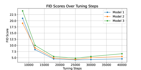
Figure 6: FID Curves during Tuning on CIFAR10

Due to the inherent variance in GPT-4’s inference, which is utilized in our proxy pruning algorithm, the importance assessments obtained are not entirely consistent. Hence, designing experiments to evaluate the stability of the pruning algorithm is of great significance. In these experiments, we pruned the CIFAR10 model with a pruning rate set at 0.7, obtaining three pruning outcomes each time. After evaluating the performance of these three sub-models, we stored the results in a memory bank for the next round of three prunings. This process was repeated for five rounds, with the results illustrated in Fig. 7. It is evident that with the enlargement of the proxy’s memory bank, the effectiveness of pruning gradually improved, and the variance in performance among models pruned in a single round was minimal, indicating strong stability in our algorithm.

5.4 Overall Efficacy Validation

After conducting ablation studies on each innovative aspect, we evaluated the overall effectiveness of our strategy. In these experiments, we continued to use IDDPM as the codebase and compared its performance on two datasets, CIFAR10 and Imagenet64, with the original performance of IDDPM. In the original training configuration of IDDPM, for CIFAR10, the FLOPs of the denoising model were 8.14G with a total training requirement of 500k steps. For Imagenet64, the denoising model’s FLOPs were 39.3G with 1.5M steps needed for training. When applying our Step-adaptive training strategy to IDDPM, we set the minimum FLOPs limit $k$ to 0.5 and the number of timestep groups to 10. For the CIFAR10 dataset, we set the training steps in the first phase to 200k, and the fine-tuning steps for each pruned group model in the second phase to 25k. For the Imagenet64 dataset, the first phase training steps were set to 0.8M, and the fine-tuning steps in the second phase to 50k. The results are presented in Tab. 1.

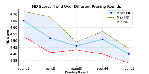
Figure 7: Mean-std Curve over Pruning Rounds

The experimental results demonstrate that, compared to traditional diffusion model training strategies, our training strategy not only achieves faster convergence and reduces overall training expenses but also enhances model performance with lower average FLOPs. Also, this training approach is compatible with various improvements in diffusion models, fostering enhanced performance across a spectrum of diffusion models.

6 Conclusion

In this paper, we introduce a two-stage divide-and-conquer strategy specifically designed for diffusion models. This approach enhances the performance of diffusion models by assigning customized models to different time steps, thereby mitigating training conflicts and accelerating convergence. Our experiments demonstrate that with the addition of this algorithm, the FID of IDDPM on CIFAR-10 improved from 4.08 to 3.52, using only 56% of the training steps. To further tailor the models, we propose a GPT-4-based pruning algorithm for diffusion models. In our CIFAR-10 experiments, this pruning algorithm demonstrates an FID advantage of over 0.2 compared to other methods. The combination of the two-stage divide-and-conquer strategy and the GPT-based pruning algorithm resulted in an improvement of 0.32 and 1.5 in FID on CIFAR-10 and ImageNet64 datasets, respectively, with an approximate 20% reduction in the model’s computational requirements.

Supplementary Material

In the appendix, we present three additional experiments to further validate the effectiveness of each innovative aspect within our proposed Step-Adaptive Training Strategy.

Appendix A Comparative Analysis: Single-Stage vs. Two-Stage Training Strategies

To further validate the effectiveness of the two-stage training in our training strategy, we conducted an experiment with a single-stage divide-and-conquer training strategy. Specifically, we maintained the same group and training configurations on CIFAR-10 as in the experiment described in Sec. 5.1, but we abandoned the two-stage training. Instead, we trained models for each group from scratch.

The experimental results are shown in Fig. 8. With two-stage training, we achieved an FID of 3.52 with a total of 280k training steps. In contrast, with single-stage training, the FID was only 52.8 even after 300k training steps. This demonstrates that the two-stage training in our strategy significantly speeds up the overall training of the model, reducing training costs. At the optimal performance point, the total number of training steps reached 600k, but the FID was only 4.81, which is far inferior to the 3.52 and even worse than the original IDDPM. We believe this is mainly due to the fact that the models at each time-step group were independently trained from scratch, resulting in a lack of coordination among the models and adversely affecting the overall model performance.

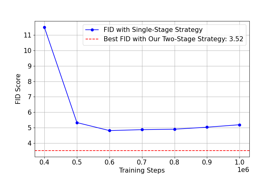
Figure 8: Comparative FID Scores: Single-Stage vs. Two-Stage Strategies in IDDPM on CIFAR10

Appendix B Group Quantity Ablation Experiment

In all the experiments conducted previously, we have consistently used 10 as the number of groups for timesteps. To investigate the impact of the number of groups on the performance of diffusion models, we conducted an exploratory experiment on CIFAR-10 regarding the quantity of groups. In this experiment, we did not prune the model. Instead, similar to the experiments in Sec. 5.1, we used the same model architecture for both stages of the experiment. We set the group numbers to 4, 8, 10, 15 and 20, respectively, and the results are presented in Tab. 5.

It is observed that as the number of groups increases, the performance of the model initially improves and then deteriorates. With fewer than 10 groups, an increase in the number of groups enhances the specialization of the denoising model, leading to an overall performance improvement of the diffusion model. However, when the group count exceeds 10, further increasing the number of groups causes the denoising model to become overly specialized, reducing its collaborative capability and consequently diminishing the overall performance of the diffusion model. Therefore, 10 is identified as a reasonable number of groups.

Table 5: FID Changes for Different Group Numbers in IDDPM

Group Number	4	8	10	15	20
FID	3.62	3.56	3.52	3.56	3.60

Appendix C Pruning Algorithm Ablation Experiment

In Sec. 5.3, we empirically demonstrated that our proposed Proxy-based pruning method outperforms other pruning algorithms in diffusion models. To explore the extent to which replacing the pruning algorithm affects the overall performance of the model within our Step-adaptive training strategy, we designed a comparative experiment on CIFAR-10: keeping other configurations constant, we substituted the pruning algorithm with random pruning and magnitude pruning. The experimental results are presented in Tab. 6. It is evident that after changing the pruning algorithm, the performance of the model slightly decreased compared to the model obtained with the original Step-adaptive training strategy, but still outperformed the original IDDPM.

Table 6: Performance Comparison of Different Models

Model Description	FID	FLOPs	Parameters
Original IDDPM	4.08	8.14G	52.5M
+Our Training(Random)	3.95	6.71G	46.6M
+Our Training(Magnitude)	3.88	6.75G	47.3M
+Our Training(Proxy)	3.76	6.56G	48.7M

References

- Bao et al. [2022] Fan Bao, Chongxuan Li, Jun Zhu, and Bo Zhang. Analytic-dpm: an analytic estimate of the optimal reverse variance in diffusion probabilistic models. arXiv preprint arXiv:2201.06503, 2022.
- Cai et al. [2023] Yuzhe Cai, Shaoguang Mao, Wenshan Wu, Zehua Wang, Yaobo Liang, Tao Ge, Chenfei Wu, Wang You, Ting Song, Yan Xia, et al. Low-code llm: Visual programming over llms. arXiv preprint arXiv:2304.08103, 2023.
- Creswell et al. [2018] Antonia Creswell, Tom White, Vincent Dumoulin, Kai Arulkumaran, Biswa Sengupta, and Anil A Bharath. Generative adversarial networks: An overview. IEEE signal processing magazine, 35(1):53–65, 2018.
- Fang et al. [2023] Gongfan Fang, Xinyin Ma, and Xinchao Wang. Structural pruning for diffusion models. arXiv preprint arXiv:2305.10924, 2023.
- Gaikwad and El-Sharkawy [2018] Akash Sunil Gaikwad and Mohamed El-Sharkawy. Pruning convolution neural network (squeezenet) using taylor expansion-based criterion. In 2018 IEEE International Symposium on Signal Processing and Information Technology (ISSPIT), pages 1–5. IEEE, 2018.
- Goodfellow et al. [2020] Ian Goodfellow, Jean Pouget-Abadie, Mehdi Mirza, Bing Xu, David Warde-Farley, Sherjil Ozair, Aaron Courville, and Yoshua Bengio. Generative adversarial networks. Communications of the ACM, 63(11):139–144, 2020.
- Han et al. [2015a] Song Han, Huizi Mao, and William J Dally. Deep compression: Compressing deep neural networks with pruning, trained quantization and huffman coding. arXiv preprint arXiv:1510.00149, 2015a.
- Han et al. [2015b] Song Han, Jeff Pool, John Tran, and William Dally. Learning both weights and connections for efficient neural network. Advances in neural information processing systems, 28, 2015b.
- Hang et al. [2023] Tiankai Hang, Shuyang Gu, Chen Li, Jianmin Bao, Dong Chen, Han Hu, Xin Geng, and Baining Guo. Efficient diffusion training via min-snr weighting strategy. arXiv preprint arXiv:2303.09556, 2023.
- Ho et al. [2020] Jonathan Ho, Ajay Jain, and Pieter Abbeel. Denoising diffusion probabilistic models. Advances in neural information processing systems, 33:6840–6851, 2020.
- Ho et al. [2022] Jonathan Ho, William Chan, Chitwan Saharia, Jay Whang, Ruiqi Gao, Alexey Gritsenko, Diederik P Kingma, Ben Poole, Mohammad Norouzi, David J Fleet, et al. Imagen video: High definition video generation with diffusion models. arXiv preprint arXiv:2210.02303, 2022.
- Huang et al. [2022] Rongjie Huang, Zhou Zhao, Huadai Liu, Jinglin Liu, Chenye Cui, and Yi Ren. Prodiff: Progressive fast diffusion model for high-quality text-to-speech. In Proceedings of the 30th ACM International Conference on Multimedia, pages 2595–2605, 2022.
- Kingma and Dhariwal [2018] Durk P Kingma and Prafulla Dhariwal. Glow: Generative flow with invertible 1x1 convolutions. Advances in neural information processing systems, 31, 2018.
- Kosiorek et al. [2021] Adam R Kosiorek, Heiko Strathmann, Daniel Zoran, Pol Moreno, Rosalia Schneider, Sona Mokrá, and Danilo Jimenez Rezende. Nerf-vae: A geometry aware 3d scene generative model. In International Conference on Machine Learning, pages 5742–5752. PMLR, 2021.
- LeCun et al. [1989] Yann LeCun, John Denker, and Sara Solla. Optimal brain damage. Advances in neural information processing systems, 2, 1989.
- Lee et al. [2020] Jaeho Lee, Sejun Park, Sangwoo Mo, Sungsoo Ahn, and Jinwoo Shin. Layer-adaptive sparsity for the magnitude-based pruning. arXiv preprint arXiv:2010.07611, 2020.
- Lei et al. [2017] Wang Lei, Huawei Chen, and Yixuan Wu. Compressing deep convolutional networks using k-means based on weights distribution. In Proceedings of the 2nd International Conference on Intelligent Information Processing, pages 1–6, 2017.
- Li et al. [2016] Hao Li, Asim Kadav, Igor Durdanovic, Hanan Samet, and Hans Peter Graf. Pruning filters for efficient convnets. arXiv preprint arXiv:1608.08710, 2016.
- Li et al. [2023] Wenhao Li, Xiu Su, Shan You, Fei Wang, Chen Qian, and Chang Xu. Diffnas: Bootstrapping diffusion models by prompting for better architectures. arXiv preprint arXiv:2310.04750, 2023.
- Lin et al. [2018] Shaohui Lin, Rongrong Ji, Yuchao Li, Yongjian Wu, Feiyue Huang, and Baochang Zhang. Accelerating convolutional networks via global & dynamic filter pruning. In IJCAI, page 8. Stockholm, 2018.
- Liu et al. [2022] Luping Liu, Yi Ren, Zhijie Lin, and Zhou Zhao. Pseudo numerical methods for diffusion models on manifolds. arXiv preprint arXiv:2202.09778, 2022.
- Liu et al. [2017] Zhuang Liu, Jianguo Li, Zhiqiang Shen, Gao Huang, Shoumeng Yan, and Changshui Zhang. Learning efficient convolutional networks through network slimming. In Proceedings of the IEEE international conference on computer vision, pages 2736–2744, 2017.
- Lu et al. [2022] Cheng Lu, Yuhao Zhou, Fan Bao, Jianfei Chen, Chongxuan Li, and Jun Zhu. Dpm-solver: A fast ode solver for diffusion probabilistic model sampling in around 10 steps. Advances in Neural Information Processing Systems, 35:5775–5787, 2022.
- Mao et al. [2023] Rui Mao, Guanyi Chen, Xulang Zhang, Frank Guerin, and Erik Cambria. Gpteval: A survey on assessments of chatgpt and gpt-4. arXiv preprint arXiv:2308.12488, 2023.
- Mao et al. [2017] Xudong Mao, Qing Li, Haoran Xie, Raymond YK Lau, Zhen Wang, and Stephen Paul Smolley. Least squares generative adversarial networks. In Proceedings of the IEEE international conference on computer vision, pages 2794–2802, 2017.
- Molchanov et al. [2016] Pavlo Molchanov, Stephen Tyree, Tero Karras, Timo Aila, and Jan Kautz. Pruning convolutional neural networks for resource efficient inference. arXiv preprint arXiv:1611.06440, 2016.
- Molchanov et al. [2019] Pavlo Molchanov, Arun Mallya, Stephen Tyree, Iuri Frosio, and Jan Kautz. Importance estimation for neural network pruning. In Proceedings of the IEEE/CVF conference on computer vision and pattern recognition, pages 11264–11272, 2019.
- Nichol et al. [2021] Alex Nichol, Prafulla Dhariwal, Aditya Ramesh, Pranav Shyam, Pamela Mishkin, Bob McGrew, Ilya Sutskever, and Mark Chen. Glide: Towards photorealistic image generation and editing with text-guided diffusion models. arXiv preprint arXiv:2112.10741, 2021.
- Nichol and Dhariwal [2021] Alexander Quinn Nichol and Prafulla Dhariwal. Improved denoising diffusion probabilistic models. In International Conference on Machine Learning, pages 8162–8171. PMLR, 2021.
- Pandey et al. [2021] Kushagra Pandey, Avideep Mukherjee, Piyush Rai, and Abhishek Kumar. Vaes meet diffusion models: Efficient and high-fidelity generation. In NeurIPS 2021 Workshop on Deep Generative Models and Downstream Applications, 2021.
- Phung et al. [2023] Hao Phung, Quan Dao, and Anh Tran. Wavelet diffusion models are fast and scalable image generators. In Proceedings of the IEEE/CVF Conference on Computer Vision and Pattern Recognition, pages 10199–10208, 2023.
- Saharia et al. [2022] Chitwan Saharia, Jonathan Ho, William Chan, Tim Salimans, David J Fleet, and Mohammad Norouzi. Image super-resolution via iterative refinement. IEEE Transactions on Pattern Analysis and Machine Intelligence, 45(4):4713–4726, 2022.
- Salimans and Ho [2022] Tim Salimans and Jonathan Ho. Progressive distillation for fast sampling of diffusion models. arXiv preprint arXiv:2202.00512, 2022.
- Simonyan and Zisserman [2014] Karen Simonyan and Andrew Zisserman. Very deep convolutional networks for large-scale image recognition. arXiv preprint arXiv:1409.1556, 2014.
- Sinha et al. [2021] Abhishek Sinha, Jiaming Song, Chenlin Meng, and Stefano Ermon. D2c: Diffusion-decoding models for few-shot conditional generation. Advances in Neural Information Processing Systems, 34:12533–12548, 2021.
- Song and Ermon [2020] Yang Song and Stefano Ermon. Improved techniques for training score-based generative models. Advances in neural information processing systems, 33:12438–12448, 2020.
- Song et al. [2021] Yang Song, Conor Durkan, Iain Murray, and Stefano Ermon. Maximum likelihood training of score-based diffusion models. Advances in Neural Information Processing Systems, 34:1415–1428, 2021.
- Vahdat et al. [2021] Arash Vahdat, Karsten Kreis, and Jan Kautz. Score-based generative modeling in latent space. Advances in Neural Information Processing Systems, 34:11287–11302, 2021.
- Wang et al. [2017] Kunfeng Wang, Chao Gou, Yanjie Duan, Yilun Lin, Xinhu Zheng, and Fei-Yue Wang. Generative adversarial networks: introduction and outlook. IEEE/CAA Journal of Automatica Sinica, 4(4):588–598, 2017.
- Wong and Li [2000] Chun Shan Wong and Wai Keung Li. On a mixture autoregressive model. Journal of the Royal Statistical Society Series B: Statistical Methodology, 62(1):95–115, 2000.
- Yang et al. [2022] Ruihan Yang, Prakhar Srivastava, and Stephan Mandt. Diffusion probabilistic modeling for video generation. arXiv preprint arXiv:2203.09481, 2022.
- Zhang et al. [2022] Qinsheng Zhang, Molei Tao, and Yongxin Chen. gddim: Generalized denoising diffusion implicit models. arXiv preprint arXiv:2206.05564, 2022.
- Zheng et al. [2023] Mingkai Zheng, Xiu Su, Shan You, Fei Wang, Chen Qian, Chang Xu, and Samuel Albanie. Can gpt-4 perform neural architecture search? arXiv preprint arXiv:2304.10970, 2023.