Ultradiscretization in discrete limit cycles
of tropically discretized and max-plus Sel’kov models

Yoshihiro Yamazaki^1∗) and Shousuke Ohmori^2,3

¹Department of Physics, Waseda University, Shinjuku, Tokyo 169-8555, Japan
²National Institute of Technology, Gunma College, Maebashi-shi, Gunma 371-8530, Japan
³Waseda Research Institute for Science and Engineering, Waseda UniversityShinjuku, Tokyo 169-8555, Japan

*corresponding author : yoshy@waseda.jp
  

Abstract
The state of limit cycles for a tropically discretized Sel’kov model becomes ultradiscrete due to phase lock caused by a saddle-node bifurcation. This property is essentially the same as the case of the negative feedback model, and existence of a general mechanism for ultradiscretization of the limit cycles is suggested. Furthermore in the case of the max-plus Selkov model, we find the logarithmic dependence of the time to pass the bottleneck for phase drift motion in the vicinity of the bifurcation point. This dependency can be understood as a consequence of the piecewise linearization by applying the ultradiscrete limit.

Recently, we have reported the results of numerical analysis for the dynamical properties of the tropically discretized negative feedback model [1, 2, 3]. This model includes a positive parameter $\tau$, which corresponds to the time interval for discretization. Discrete stable (attractive) limit cycle solutions emerge in this model when $\tau$ is larger than a finite positive value $\tau_{0}$. The interesting point is that the states (phases) of the limit cycles become ultradiscrete due to phase lock by saddle-node bifurcation at $\tau=\tau^{\ast}>\tau_{0}$. Additonally, there exist unstable (repulsive) limit cycles in addition to stable ones when $\tau>\tau^{\ast}$. Furthermore the existence of these stable and unstable ultradiscrete limit cycles is retained even in the max-plus model, which are obtained from the discretized model in the ultradiscrete limit[4].

So far the above dynamical properties have been confirmed only in the negative feedback model. It is unclear whether they hold only for the negative feedback model or more generally. In this letter, with a focus on their generality, we demonstrate another example, the tropically discretized Sel’kov model[5, 6, 7],

$$\left\{\begin{aligned} x_{n+1}&=\frac{x_{n}+\tau(ay_{n}+x^{2}_{n}y_{n})}{1+\tau}\equiv\eta(x_{n},y_{n}),\\ y_{n+1}&=\frac{y_{n}+\tau b}{1+\tau(a+x_{n}^{2})}\equiv\xi(x_{n},y_{n}).\end{aligned}\right.$$ (1)

Equation (1) can be derived from the following continuous model[8, 9] via the tropical discretization[10, 11] with the additional positive parameter $\tau$ for the discrete time step,

$$\left\{\begin{aligned} \frac{dx}{dt}&=-x+ay+x^{2}y,\\ \frac{dy}{dt}&=b-ay-x^{2}y,\end{aligned}\right.$$ (2)

where $x$, $y$, $a$, and $b$ are positive. We have already reported that eq.(1) has limit cycle solutions for all $\tau$ when we set $a=0.01$ and $b=0.98$ [5, 12]. Defining the phase $\theta_{n}(\tau)\in[0,2\pi)$ in the limit cycles as

$$\theta_{n}(\tau)=\arctan\displaystyle\frac{\ln y_{n}-\ln\bar{y}}{\ln x_{n}-\ln\bar{x}},$$ (3)

where $(\bar{x},\bar{y})$ is the fixed point of eq.(1), we obtain the bifurcation diagram of $\{\theta_{n}(\tau)\}$ shown as the blue scatter plot in Fig.1. It is clearly found that distribution of $\{\theta_{n}(\tau)\}$ changes at $\tau=\tau^{\ast}$ and that the state of the limit cycle becomes ultradiscrete when $\tau>\tau^{\ast}$.

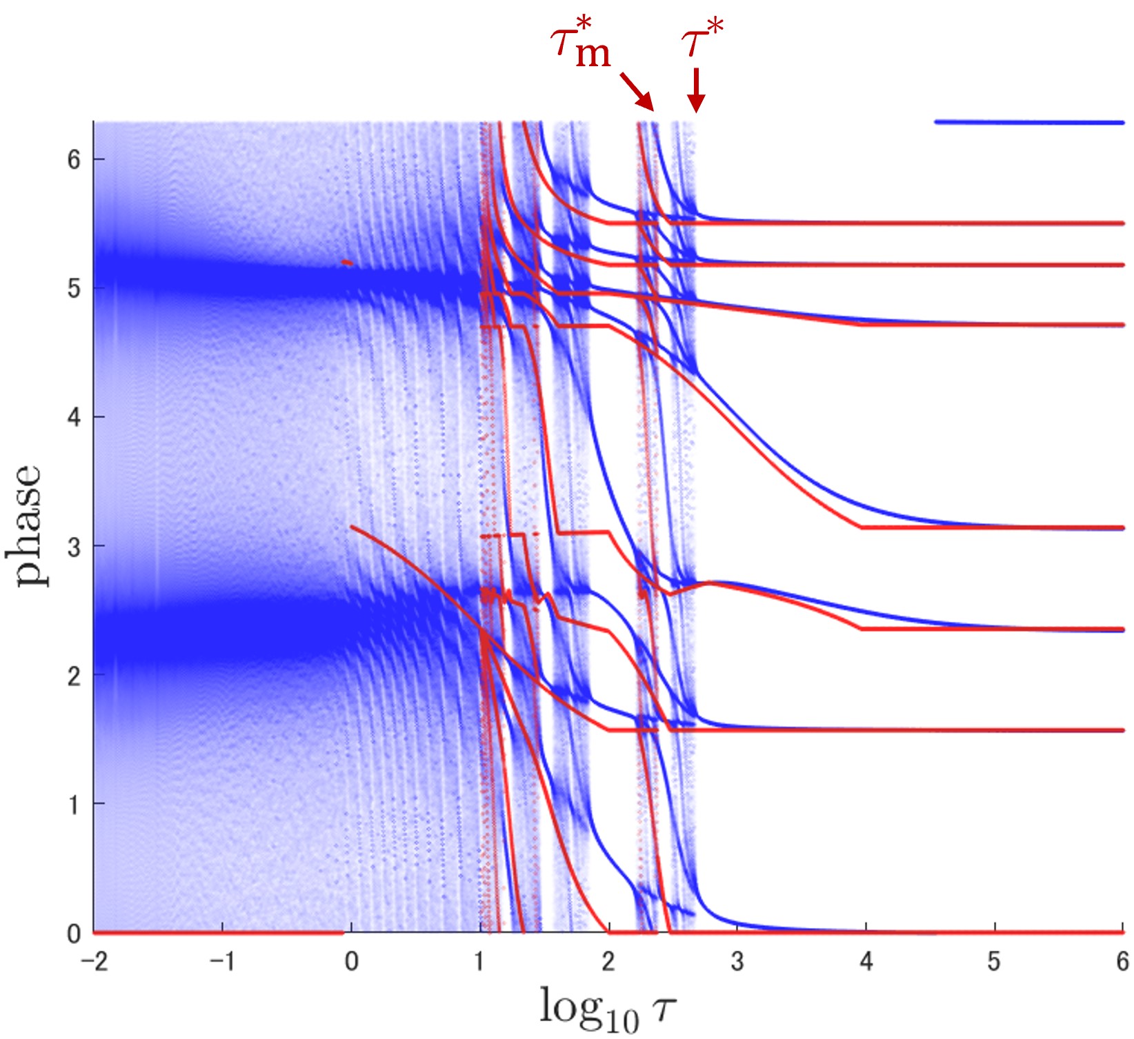
Figure 1: The blue scatter plot: the bifurcation diagram for the phase $\theta_{n}$ as a function of $\tau$ obtained from eq.(1) with $a=0.01$ and $b=0.98$. The red: the max-plus bifurcation diagram for $\Theta_{n}(\tau)$ obtained from eq.(5).

The blue plot in Fig.1 shows that the ultradiscrete limit cycle for $\tau>\tau^{\ast}$ consists of seven states. (For more discussion regarding the number of states, see ref.[6].) Here we consider the time evolution of the state at every seven steps,

$$x_{7(n+1)}=\eta^{7}(x_{7n},y_{7n}),\qquad y_{7(n+1)}=\xi^{7}(x_{7n},y_{7n}),$$ (4)

where $\eta^{7}$ and $\xi^{7}$ show 7-th iterates of $\eta$ and $\xi$ in eq.(1). We introduce the phase $\bar{\theta}_{7}$ of the fixed point $(\bar{x}_{7},\bar{y}_{7})$ from eq.(3), where $(\bar{x}_{7},\bar{y}_{7})$ satisfies $\bar{x}_{7}=\eta^{7}(\bar{x}_{7},\bar{y}_{7})$ and $\bar{y}_{7}=\xi^{7}(\bar{x}_{7},\bar{y}_{7})$. Based on eq.(4), we can numerically estimate the values of $\tau^{\ast}$ as $\tau^{\ast}\approx 473.439297\cdots$ by the upper limit value for absence of the fixed points. We obtain 14 fixed points when $\tau>\tau^{\ast}$ and the phases obtained from them are shown in Fig.2 as a function of $\tau$. It is noted that 7 phases with the blue open circles, denoted by $\left\{\bar{\theta}_{7}^{\rm{(s)}}\right\}$ hereafter, are identical to the ultradiscrete states for $\tau>\tau^{\ast}$ shown by the blue plot in Fig.1. The other 7 phases with the red asterisks are denoted by $\left\{\bar{\theta}_{7}^{\rm{(u)}}\right\}$.

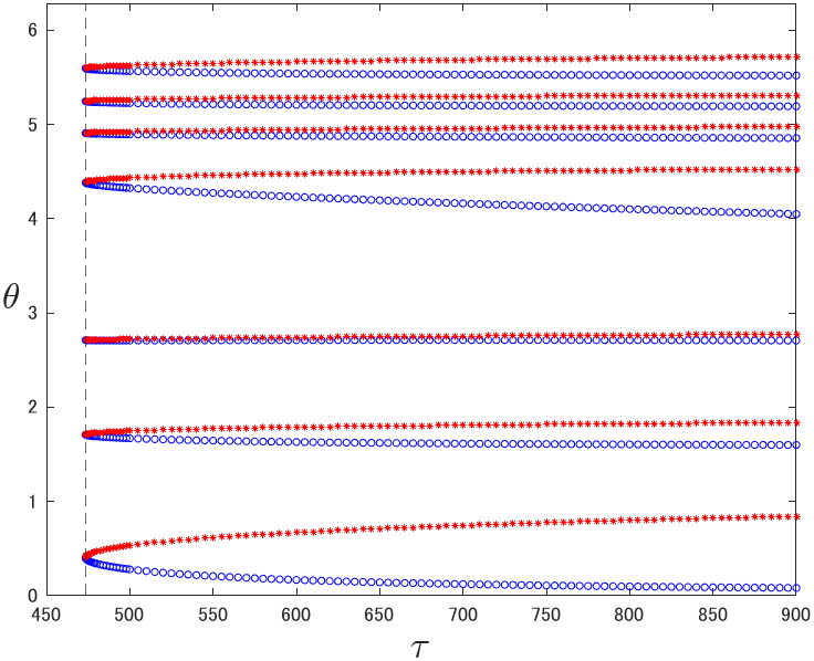
Figure 2: The phases $\bar{\theta}_{7}$ for the fixed points $(\bar{x}_{7},\bar{y}_{7})$ of eq.(4) as a function of $\tau$.

For the stability of these fixed points, the eigenvalues of their Jacobi matrix are focused on. Figure 3(a) shows the maximum eigenvalues $\lambda_{7}^{\rm(s)}$ (blue circles) and $\lambda_{7}^{\rm(u)}$ (red asterisks) for $\left\{\bar{\theta}_{7}^{\rm{(s)}}\right\}$ and $\left\{\bar{\theta}_{7}^{\rm{(u)}}\right\}$, respectively. It is concluded from this figure that $\left\{\bar{\theta}_{7}^{\rm{(s)}}\right\}$ are stable and $\left\{\bar{\theta}_{7}^{\rm{(u)}}\right\}$ are unstable, and that saddle-node bifurcation occurs at $\tau=\tau^{\ast}$. In addition, Fig.3(b) shows the asymptotic property for $\tau$ dependence of $\lambda_{7}^{\rm{(s)}}$ and $\lambda_{7}^{\rm{(u)}}$: $|\lambda_{7}^{\rm{(s)}}-1|,|\lambda_{7}^{\rm{(u)}}-1|\sim(\tau-\tau^{\ast})^{0.5}$. These dynamical properties for ultradiscretization of the Sel’kov model are essentially the same as the case of the negative feedback model, though the number of the ultradiscrete states is different.

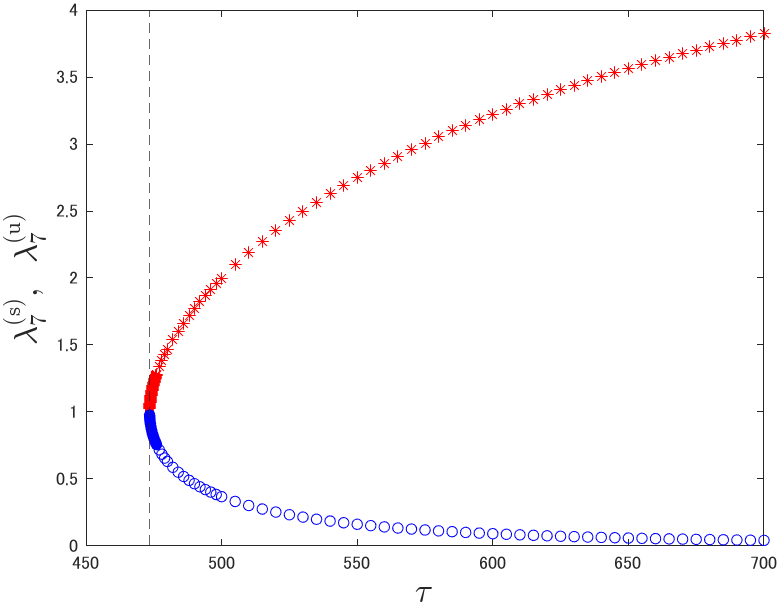
(a)

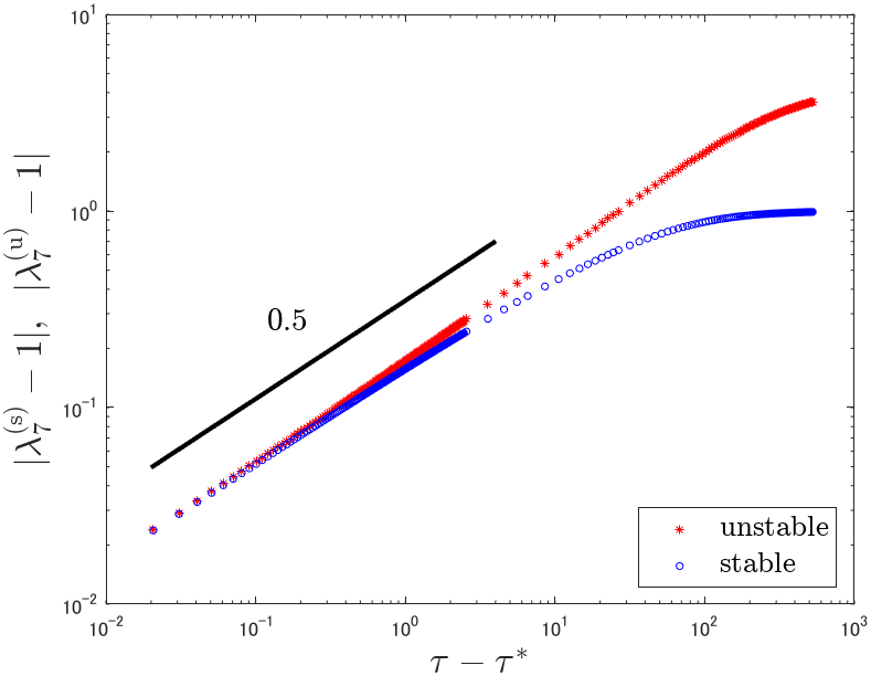
(b)

Figure 3: (a) The maximum eigenvalues $\lambda_{7}^{\text{(s)}}$ (blue circle) and $\lambda_{7}^{\text{(u)}}$ (red asterisk) of the Jacobi matrix for the fixed points $\{\bar{\theta}_{7}^{\rm{(s)}}\}$ and $\{\bar{\theta}_{7}^{\rm{(u)}}\}$, respectively. (b) The scaling relations between $\lambda_{7}^{\text{(s)}}$, $\lambda_{7}^{\text{(u)}}$ and $\tau-\tau^{\ast}$.

Applying the variable transformations, $\tau=e^{T/\varepsilon}$, $x_{n}=e^{X_{n}/\varepsilon}$, $y_{n}=e^{Y_{n}/\varepsilon}$, $a=e^{A/\varepsilon}$, $b=e^{B/\varepsilon}$, and then the ultradiscrete limit[4],

$$\lim_{\varepsilon\to 0}\varepsilon\ln\left(e^{\frac{P}{\varepsilon}}+e^{\frac{Q}{\varepsilon}}+\cdots\right)=\max(P,Q,\cdots),$$

to eq.(1), we obtain

$$\left\{\begin{aligned} X_{n+1}&=\max(X_{n},T+\max(A+Y_{n},2X_{n}+Y_{n}))-\max(0,T),\\ Y_{n+1}&=\max(Y_{n},T+B)-\max(0,T+\max(A,2X_{n})).\end{aligned}\right.$$ (5)

Between the variables in eq.(1) and eq.(5), the following relations hold: $X_{n}=\ln x_{n}$, $Y_{n}=\ln y_{n}$, $T=\ln\tau$, $A=\ln a$, and $B=\ln b$. Here the phase $\Theta_{n}$ for $(X_{n},Y_{n})$ is introduced as

$$\Theta_{n}=\arctan\displaystyle\frac{Y_{n}-\ln\bar{y}}{X_{n}-\ln\bar{x}}.$$ (6)

Based on eq.(5), we obtain the bifurcation diagram of $\Theta_{n}$ as a function of $\tau$. Actually, the red scatter plot in Fig.1 shows the result. As in the case of the negative feedback model, saddle-node bifurcation is retained in the max-plus system given by eq.(5). Here the saddle-node bifurcation point for eq.(5), denoted by $\tau_{\text{m}}^{\ast}$, was numerically estimated as $\tau_{\text{m}}^{\ast}\approx 239.29993555\cdots$.

Figure 4(a) shows the phase drift and bottleneck motion for the phase every 7 steps, $\theta_{7}$, when $\tau\lesssim\tau^{\ast}$ in eq.(1). As a scaling property for the average time to pass through the bottlenecks, denoted by $T_{\rm{b.n.}}$, we can confirm $T_{\rm{b.n.}}\sim(\tau^{\ast}-\tau)^{-0.5}$ from Fig.4(b). In the max-plus case of eq.(5), the phase drift and bottleneck motion for the phase every 7 steps, $\Theta_{7}$, can be also observed as shown in Fig.5(a) when $\tau\lesssim\tau_{\text{m}}^{\ast}$. The fact that the bottleneck motion is retained in the max-plus system is a common property in the Sel’kov model and the negative feedback model. Moreover, as shown in Fig.5(b), we have newly found the logarithmic relation, $T_{\rm{b.n.}}\sim-\ln(\tau_{\text{m}}^{\ast}-\tau)$, in the max-plus case, which is different scaling relation from the discrete case.

Comparing Fig.4(b) and Fig.5(b), it is interesting that the ultradiscrete limit brings about the change of the scaling property for $T_{\rm{b.n.}}$. The reason for the logaritmic dependence of $T_{\rm{b.n.}}$ on $(\tau_{\text{m}}^{\ast}-\tau)\equiv\lambda$ in the max-plus system can be explained as follows. The parameter $\lambda$ corresponds to the characteristic size of bottleneck threshold. Important point is that the time evolution of the states becomes piecewise linear by taking the ultradiscrete limit. Then the initial state approaches the bottleneck at the constant contraction ratio $r(<1)$ for each time step. Therefore, the time step $T_{\rm{b.n.}}$ satisfying $r^{T_{\rm{b.n.}}}\sim\lambda$ is what we desire. Since $\ln r<0$, we obtain $T_{\rm{b.n.}}\sim-\ln(\tau_{\text{m}}^{\ast}-\tau)$. Note that we have also confirmed that this logarithmic dependence also holds for the max-plus negative feedback model.

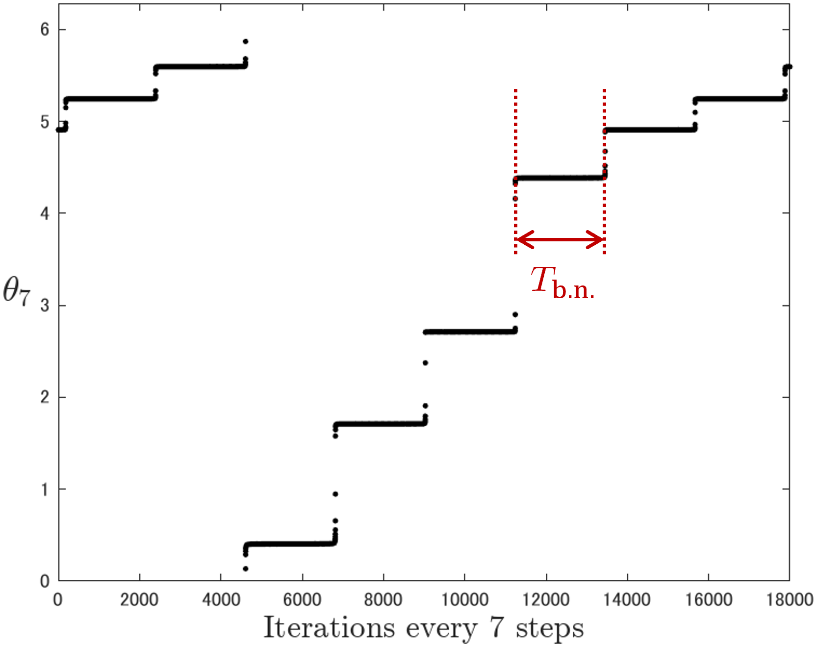
(a)

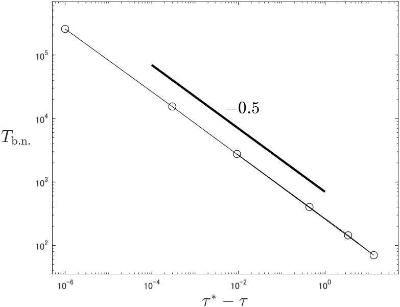
(b)

Figure 4: (a) The bottleneck motion of $\theta_{7}$ for $\tau\lesssim\tau^{\ast}$ obtained from eq.(1). We set $\tau=473.439$. (b) The scaling relation between $T_{\rm{b.n.}}$ and $\tau^{\ast}-\tau$.

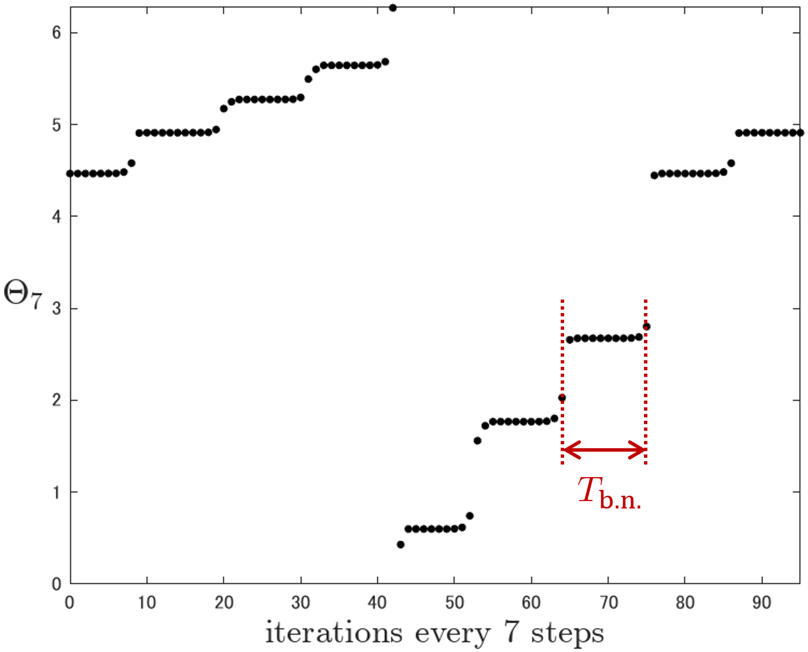
(a)

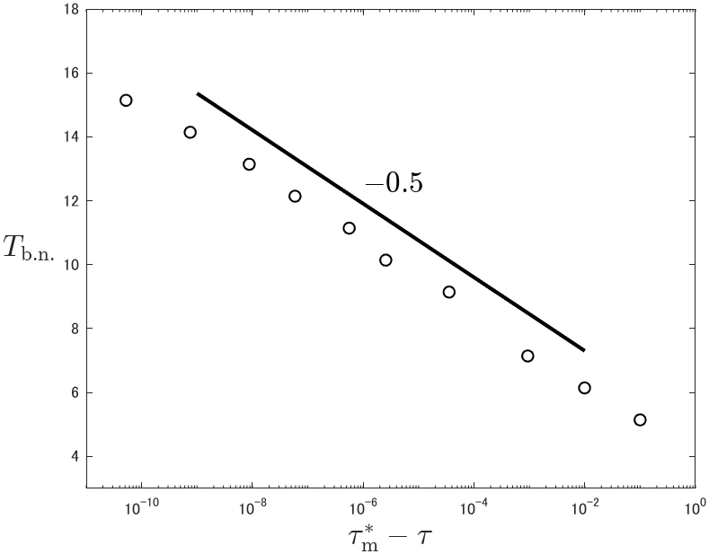
(b)

Figure 5: (a) The max-plus bottleneck motion of $\Theta_{7}$ for $\tau\lesssim\tau^{\ast}$ obtained from eq.(5). We set $\tau=239.299935$. (b) The logarithmic dependence of $T_{\rm{b.n.}}$ on $\tau_{\text{m}}^{\ast}-\tau$.

Finally we comment on the possibility of general treatment for their dynamical properties by comparing the negative feedback model and the Sel’kov model. For eq.(5), considering a sufficiently large $T$ (or $T\to\infty$) and the following variable transformations, $\displaystyle X_{n}-\frac{A}{2}\to X_{n}$, $\displaystyle Y_{n}+\frac{A}{2}\to Y_{n}$, and $\displaystyle B-\frac{A}{2}\to B$, we obtain the simplified max-plus Sel’kov model[5, 6, 7],

$$\left\{\begin{aligned} X_{n+1}&=Y_{n}+\max(0,2X_{n}),\\ Y_{n+1}&=B-\max(0,2X_{n}).\end{aligned}\right.$$ (7)

On the other hand, regarding the negative feedback model[1, 2, 3],

$$\left\{\begin{aligned} \frac{dx}{dt}&=y-x,\\ \frac{dy}{dt}&=\frac{1}{1+x^{m}}-\frac{y}{b},\end{aligned}\right.$$ (8)

from its tropically discretized one,

$$\left\{\begin{aligned} x_{n+1}&=\frac{x_{n}+\tau y_{n}}{1+\tau},\\ y_{n+1}&=\frac{y_{n}+\frac{\tau}{1+x_{n}^{m}}}{1+\frac{\tau}{b}},\end{aligned}\right.$$ (9)

we can obtain the following simplified max-plus negative feedback model[1, 2],

$$\left\{\begin{aligned} X_{n+1}&=Y_{n},\\ Y_{n+1}&=B-\max(0,2X_{n}),\end{aligned}\right.$$ (10)

by the same treatment as the Sel’kov model. Therefore, it is natural to adopt the following equation as a more general set of equations involving both eq.(7) and eq.(10),

$$\left\{\begin{aligned} X_{n+1}&=Y_{n}+\max(0,RX_{n}),\\ Y_{n+1}&=B-\max(0,SX_{n}).\end{aligned}\right.$$ (11)

The dynamical properties of the max-plus system given by eq.(11) will be reported elsewhere.

In conclusion, our research has demonstrated that the emergence of ultradiscrete states, induced by phase locking as a result of saddle-node bifurcation in discrete limit cycles, is not exclusive to the negative feedback model but is also observable in the Sel’kov model. Moreover, a comparison between the simplified max-plus models presented in eq.(7) and eq.(10) reveals a striking similarity, despite the apparent divergence in the corresponding original continuous models. Additionally, it has been found that the logarithmic relationship governing the average time required for a phase to pass through the bottleneck in the max-plus system stems from the piecewise linearization of the tropically discretized dynamical systems. These findings lead us to propose that the occurrence of ultradiscrete states due to phase locking could be a prevalent characteristic in various other models.

Acknowledgement
The authors are grateful to Prof. M. Murata, Assoc. Prof. K. Matsuya, Prof. D. Takahashi, Prof. R. Willox, Prof. H. Ujino, Prof. T. Yamamoto, and Prof. Emeritus A. Kitada for useful comments and encouragements. This work was supported by JSPS KAKENHI Grant Numbers 22K13963 and 22K03442.

References

- [1] Y. Yamazaki and S. Ohmori, Emergence of ultradiscrete states due to phase lock caused by saddle-node bifurcation in discrete limit cycles, PTEP, 2023 (2023), 081A01.
- [2] S. Ohmori and Y. Yamazaki, Dynamical properties of discrete negative feedback models, arXiv:2305.05908 [nlin.CD].
- [3] S. Gibo and H. Ito, Discrete and ultradiscrete models for biological rhythms comprising a simple negative feedback loop, J. Theor. Biol., 378 (2015), 89–95.
- [4] T. Tokihiro, Ultradiscrete Systems (Cellular Automata), in Discrete Integrable Systems (edited by B. Grammaticos, T. Tamizhmani, and Y. Kosmann-Schwarzbach, Springer, Berlin, Heidelberg, 2004), 383–424.
- [5] S. Ohmori and Y. Yamazaki, Dynamical properties of max-plus equations obtained from tropically discretized Sel’kov model, arXiv:2107.02435v1 [nlin.CD].
- [6] Y. Yamazaki and S. Ohmori, Periodicity of limit cycles in a max-plus dynamical system, J. Phys. Soc. Jpn., 90 (2021), 103001.
- [7] S. Ohmori and Y. Yamazaki, Poincaré map approach to limit cycles of a simplified ultradiscrete Sel’kov model, JSIAM Lett., 14 (2022), 127–130.
- [8] E. E. Sel’kov, Self-oscillations in glycolysis, Eur. J. Biochem., 4 (1968), 79–86.
- [9] Steven. H. Strogatz, Nonlinear Dynamics and Chaos: With Applications to Physics, Biology, Chemistry, and Engineering, 2nd ed., Westview Press, Cambridge, 2015.
- [10] M. Murata, Tropical discretization: ultradiscrete Fisher-KPP equation and ultradiscrete Allen-Cahn equation, J. Differ. Equ. Appl., 19 (2013), 1008–1021.
- [11] K. Matsuya and M. Murata, Spatial pattern of discrete and ultradiscrete Gray-Scott model, Discrete Contin. Dyn. Syst. B, 20 (2015), 173–187.
- [12] S. Ohmori and Y. Yamazaki, Types and stability of fixed points for positivity-preserving discretized dynamical systems in two dimensions, JSIAM Lett., 15 (2023), 73–76.