Relating absorbing and hard wall boundary conditions for active particles

Abstract

The connection between absorbing boundary conditions and hard walls is well established in the mathematical literature for a variety of stochastic models, including for instance the Brownian motion. In this paper we explore this duality for a different type of process which is of particular interest in physics and biology, namely active particles. For a general model of an active particle in one dimension, we provide a relation between the exit probability, i.e. the probability that the particle exits an interval from a given boundary before a certain time $t$, and the cumulative distribution of its position in the presence of hard walls at the same time $t$. We illustrate this relation for a run-and-tumble particle in the stationary state by explicitly computing both quantities.

1 Introduction

Recently, there has been a surge of interest in first passage properties of active particles. Inspired from biological systems such as bacteria, active particles exhibit a persistent motion. Unlike their passive counterparts, such as Brownian motion, they can convert energy from their environment into motion, and are thus inherently out-of-equilibrium [1, 2, 3, 4, 5]. Recently, active particles have been the focus of extensive research, leading to the development of various models like the active Ornstein-Uhlenbeck particle (AOUP) [6, 7], the active Brownian particle (ABP) [4, 8], or the run-and-tumble particle (RTP) [9, 10] (also called persistent random walk [11, 12, 13]). This last process is inspired from the motion of Escherichia coli [14] and consists in a series of straight runs over exponentially distributed times separated by instantaneous tumbles, during which the particle takes a random orientation. When confined within a specific geometry, or inside an external potential, due to this persistence, active particles tend to accumulate at the boundaries of the accessible domain [15, 16, 17, 18, 19, 20, 21]. Specifically, the distribution of the position of a one-dimensional RTP inside a confining potential has been observed to display a non-Boltzman steady state [22, 23, 24], transitioning from a passive-like regime to an active-like regime depending on the persistence time [22].

Characterizing the first passage properties [25, 26, 27] of active particles is of significant importance. For instance, understanding how small organisms navigate toward targets like food, or how sperm seek an egg cell presents a substantial challenge [28, 29, 30]. Extracting these properties for active particles proves immensely difficult, primarily due to the persistence of their motion stemming from the colored nature of their stochastic noise – being correlated in time, unlike white noise [31]. In the case of a free RTP in 1d, the survival probability and mean first time (MFPT) have been computed in various settings [24, 32, 33, 34, 35, 36]. Recently, the MFPT of a one-dimensional RTP in confining potentials has been explicitly calculated, revealing that the MFPT can be minimised with respect to the tumbling rate $\gamma$ [37]. Other studies focus on a free RTP in confined domains with various boundary conditions, in one dimension [38, 39, 40] or higher [41, 42, 43]. A related quantity is the exit probability (or splitting/hitting probability [32, 44, 45]). Imagine two absorbing walls located at $x=a$, and $x=b$ (where $b>a$), and suppose that the RTP initiates its motion at some position $x$ in $[a,b]$. What is the probability that the particles is first absorbed at the right wall $x=b$ ? The finite time counterpart of this quantity (i.e. the probability of reaching $x=b$ before time $t$) is key as it contains all first passage properties of the system. Indeed, if one knows the probability that the particle exits at $x=a$ and the probability that it exits at $x=b$ at any time, one can deduce the survival probability at all times.

We consider a generic model of active particle with two types of boundary conditions, represented in Figure 1: absorbing walls and hard walls. When a particle reaches an absorbing wall it remains stuck to it indefinitely. Conversely, a hard wall can be considered as an infinite potential step, i.e. when a particle encounters it, it remains there until its total velocity changes sign. The aim of this paper is to highlight the surprising connection which exists between these two types of boundary conditions. More precisely, the exit probability of an active particle can be related to its cumulative distribution in the presence of hard walls. This kind of relation has been shown for various types of models in the mathematical literature, where it is known as Siegmund duality [46, 47, 48, 49, 50]. Consider for instance a Brownian motion inside a potential $V(x)$, starting at position $x\in[a,b]$. The probability that it exits the interval through $x=b$ is given by $\int_{a}^{x}dz\,e^{\frac{V(z)}{T}}/\int_{a}^{b}dz\,e^{\frac{V(z)}{T}}$ (where $T$ is a diffusion constant), which is also the cumulative distribution with hard walls at $a$ and $b$, if the potential is $-V(x)$ (as noticed for instance in [45]). Our work extends this duality to active particles.

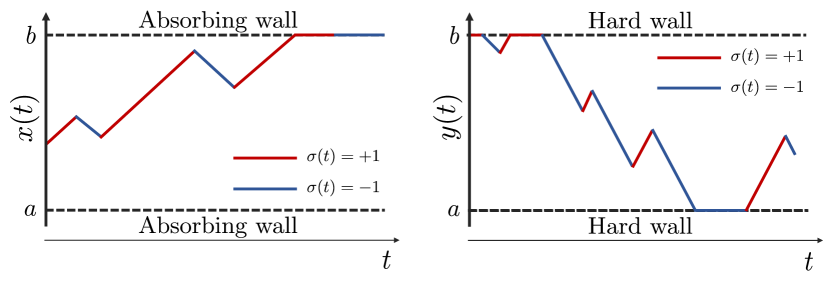
Figure 1: We consider a RTP that evolves through the equation of motion $\dot{x}(t)=F(x)+v_{0}\,\sigma(t)$, where $\sigma(t)$ is a telegraphic noise switching from values $+1$ to $-1$ at exponentially distributed times. On the left panel we show a schematic trajectory of an RTP with absorbing walls located at $a$ and $b$. When the RTP reaches one of these walls, it will stay there forever no matter its state $\sigma=\pm 1$. On the right panel, we show a trajectory of another RTP $y(t)$, with hard walls (i.e. if the particle reaches one of the walls and tries to cross it, it stays in the same place).

The first section of this paper is devoted to the introduction of this duality for general models of active particles. We then illustrate this relation in the case of an RTP by computing independently both quantities, in the stationary state. In Section 3, we derive the exit probability (at infinite time) for an RTP with an arbitrary external force. This computation was performed before in [32] but only for a free RTP (although with an additional Brownian noise). In Section 4, we calculate the cumulative distribution of the position of an RTP when these walls are hard walls (drawing inspiration from [19, 22]).

Although we focus here on the case of active particles, this duality relation is actually much more general, and holds for other models such as diffusing diffusivity models [51, 52] or stochastic resetting [53, 54], and even some instances of discrete and continuous time random walks. All the results presented here for active particles will be derived in this more general context in an upcoming paper [55].

2 A duality relation for active particles

We consider the process $x(t)$ on a $1$d line with absorbing walls located at $x=a$ and $x=b$, where $b>a$. If the particle reaches one of these walls at any point in time, it will remain there indefinitely. The particle is initially placed inside the box such that $x(0)\in[a,b]$. In addition, the particle is subjected to an external force $F(x)$. The equation of motion is given by:

$$\dot{x}(t)=F(x)+\alpha(x)\,v(t)+\sqrt{2\,T}\,\xi(t)\,,$$ (1)

where $\xi(t)$ is a Gaussian white noise with $\langle\xi(t^{\prime})\xi(t)\rangle=\delta(t-t^{\prime})$, and $T$ is a diffusion coefficient. In Eq. (1), $v(t)$ is a stochastic process that verifies the following properties:

1. $v(t)$ is a Markov process independent of the position $x$, with propagator $G(v,t|v_{0})$.

2. $v(t)$ admits an equilibrium distribution $p_{\text{eq}}(v)$ which satisfies the detailed balance condition

   $$p_{\text{eq}}(v_{1})\,G(v_{2},t|v_{1})=p_{\text{eq}}(v_{2})\,G(v_{1},t|v_{2})\;.$$ (2)

It can be modulated by a space-dependent amplitude $\alpha(x)$.

The process described by Eq. (1) is a very general model that encompasses a wide range of stochastic processes, from passive to active particles. For example, when $\alpha(x)=0$ the resulting process $x(t)$ is simply a Brownian motion with an external force $F(x)$. Alternatively, fixing $\alpha(x)=1$ and $v(t)$ to be an Ornstein-Uhlenbeck process results in an Active Ornstein-Uhlenbeck particle (AOUP). One can also recover the run-and-tumble particle (RTP) model (potentially with a space-dependent velocity) by taking $\alpha(x)=v_{0}(x)$ and $v(t)=\sigma(t)$, where $\sigma(t)$ is the telegraphic noise that switches between values $+1$ and $-1$ with a rate $\gamma$ (see Eq. (12)).

We introduce the dual process of $x(t)$, denoted $y(t)$, with hard walls at $x=a$ and $x=b$ and $y(0)\in[a,b]$. The evolution of $y(t)$ is governed by the equation

$$\dot{y}(t)=-F(y)+\alpha(y)\,\tilde{v}(t)+\sqrt{2\,T}\,\xi(t)\,,$$ (3)

where $\tilde{v}(t)$ is a Markov process with propagator $\tilde{G}(\tilde{v},t|\tilde{v}_{0})=G(-\tilde{v},t|-\tilde{v}_{0})$. Here $\xi(t)$, denotes a different realisation of the same white noise as in (1). In the whole paper we denote with a tilde the quantities related to the process $y(t)$. Note that if $v$ is symmetric, i.e. $G(-v,t|-v_{0})=G(v,t|v_{0})$, then $\tilde{v}(t)$ and $v(t)$ have the same law and (1) and (3) differ only in the sign of the force. This is the case for all the examples of processes given above (but not for instance for a RTP with different rates for the transitions $+\to-$ and $-\to+$).

One can define the exit probability of $x(t)$ as

$$E_{b}(x,v,t)=\mathbb{P}(x(t)=b|x(0)=x,v(0)=v)\,.$$ (4)

This is the probability that the process $x(t)$ reaches $x=b$ before time $t$ (since the particle stays at $b$ once it touches it). For the dual $y(t)$ we introduce

$$\tilde{\Phi}(y,t|v;b)=\tilde{\mathbb{P}}(y(t)\leq y|\tilde{v}(t)=v;y(0)=b,\tilde{v}(0)^{eq})\,,$$ (5)

where the notation $\tilde{v}(0)^{eq}$ means that $\tilde{v}(0)$ is drawn from the equilibrium distribution $p_{\text{eq}}(v)$. This is the cumulative distribution of $y(t)$ conditioned on the value of $v(t)$, with the initial conditions $y(0)=b$, and $v(0)$ drawn at equilibrium.

It is then possible to show the identity (see [55])

$$E_{b}(x,v,t)=\tilde{\Phi}(x,t|\tilde{v}(t)=-v;b)\;.$$ (6)

This means that the probability that the process $x(t)$ reaches the boundary $x=b$ before time $t$ when initialised at $x(0)=x$ with $v(0)=v$, is equal to the probability of finding the dual process $y(t)$ within the interval $[a,x]$ at time $t$, conditioned on $\tilde{v}(t)=-v$ and given the initial condition $y(0)=b$. Of course, the relation (6) has an equivalent for the exit probability at $x=a$, $E_{a}(x,v,t)$, which can be immediately deduced by symmetry (one simply needs to revert the inequality in the definition of $\tilde{\Phi}$ and to choose $y(0)=a$).

In some cases the initial value of $v(t)$ may be unknown, or the cumulative of $y(t)$ conditioned on the velocity may be hard to compute. In this case, assuming that $v(0)$ is drawn from its equilibrium distribution $p_{\text{eq}}(v)$, we define

$$E_{b}(x,t)=\int dv\,p_{\text{eq}}(v)E_{b}(x,v,t)\;,$$ (7)

as well as

$$\tilde{\Phi}(y,t|b)=\tilde{\mathbb{P}}(y(t)\leq y|y(0)=b,\tilde{v}(0)^{eq})\,.$$ (8)

Averaging both sides of (6) over $p_{\text{eq}}(v)$ we obtain

$$E_{b}(x,t)=\tilde{\Phi}(x,t|b)\;.$$ (9)

One may also want to consider the large time limit of (6). If $y(t)$ admits a unique stationary distribution, writing $E_{b}(x,v)=E_{b}(x,v,t\to\infty)$ and $\tilde{\Phi}(x|v)=\tilde{\Phi}(x,t\to\infty|v)$, it becomes

$$E_{b}(x,v)=\tilde{\Phi}(x|v)\,.$$ (10)

In the next sections, we will illustrate this last identity in the case of RTPs by explicitly computing both sides of (10).

The duality identity (6) can be thought of as a sort of time reversal. For every trajectory of a particle starting at $x$ in the presence of a potential $V(x)$ and exiting at $b$ before or at time $t$, one can construct a trajectory of a dual particle starting at $b$ with a reversed potential $-V(x)$ and located inside $[a,x]$ at time $t$. This becomes clearer when deriving the duality relation Eq. (6) in discrete-time as done in [55].

This duality relation has several practical applications. From an analytical point of view, deriving one of the two quantities gives directly access to the other as a byproduct. Sometimes, one of them is easier to derive than the other as we will show with the RTP. If instead one seeks to compute these quantities from numerical simulations or experiments, there might be situations where one quantity is simpler to obtain than the other. For instance if one is interested in the exit probability at infinite time, one a priori needs to observe many trajectories starting from every position $x$ in $[a,b]$. Instead, one can compute the stationary distribution between hard walls by observing a single trajectory and averaging over time (assuming that the system is ergodic). This could be of particular relevance in experiments, where it is often easier to observe a single long trajectory (see e.g. Ref. [56]).

3 Exit probability of a run-and-tumble particle

We consider an RTP subjected to a force $F(x)$, that may derive from a potential $V(x)$ through the relation $F(x)=-V^{\prime}(x)$. The dynamics is as follows,

$$\frac{dx(t)}{dt}=F(x)+v_{0}\,\sigma(t)\,,$$ (11)

where $v_{0}$ is the inner speed of the particle. The telegraphic noise $\sigma(t)$ switches value at rate $\gamma$ through

$$\sigma(t+dt)=\begin{cases}\sigma(t)&\text{, with probability }(1-\gamma\,dt)\\ -\sigma(t)&\text{, with probability }\gamma\,dt\end{cases}\,.$$ (12)

The transitions between these values are referred to as tumbles. The time duration $\tau$ between two consecutive tumbles follows an exponential distribution with a probability density function given by $p(\tau)=\gamma\,e^{-\gamma\tau}$. When the RTP is in the positive state $\sigma=+1$, we describe the particle as being in a “positive” ($+$) state, whereas when it is in the negative state $\sigma=-1$, we refer to it as being in a “negative” ($-$) state. Its initial position is $x(0)=x\in[a,b]$ and two absorbing walls are located at $x=a$ and $x=b$ (see Figure 1). In this section, we will assume that $|F(x)|<v_{0}$ on the interval $[a,b]$ such that the whole interval is accessible to the particle no matter its starting position. When the force has turning points $F(x)=\pm v_{0}$, the behaviour of the particle is more subtle. We comment on such cases in Section 6. We define the probability for the RTP to exit at wall $b$ with a positive (resp. negative) initial velocity as

$$E_{b}(x,\pm)=\mathbb{P}\left(x(t\!=\!+\infty)=b\,|\,x(0)=x,\sigma(0)=\pm 1\right)\,.$$ (13)

As we assume $\sigma(0)=+1$ or $\sigma(0)=-1$ with probability $1/2$, the exit probability of an RTP regardless of the initial speed is

$$E_{b}(x)=\frac{1}{2}\left(E_{b}(x,+)+E_{b}(x,-)\right)\,.$$ (14)

We can write a pair of coupled first-order differential equations for $E_{b}(x,\pm)$. Let us evolve the particle during the time interval $[0,dt]$ and average over the possible trajectories. Suppose the RTP starts its motion at $x$, then for the positive state of the RTP, the only possible events are that the particle switches sign, with probability $\gamma\,dt$, and moves from $x$ to $x+\left[F(x)-v_{0}\right]\,dt$, or that it moves over a distance $\left[F(x)+v_{0}\right]\,dt$ while staying in the positive state, with probability $1-\gamma dt$. This translates to

$$E_{b}(x,+,t+dt)=(1-\gamma dt)\,E_{b}(x+\left[F(x)+v_{0}\right]\,dt,+,t)+\gamma dtE_{b}(x+\left[F(x)-v_{0}\right]\,dt,-,t)\,.$$ (15)

After Taylor-expanding at order $dt$, we obtain

$$\partial_{t}E_{b}(x,+,t)=\left[F(x)+v_{0}\right]\partial_{x}E_{b}(x,+,t)+\gamma E_{b}(x,-,t)-\gamma E_{b}(x,+,t)\,,$$ (16)

and similarly for $E_{b}(x,-,t+dt)$. Taking the infinite time limit, it yields

$$\left[F(x)+v_{0}\right]\partial_{x}E_{b}(x,+)+\gamma\,E_{b}(x,-)-\gamma\,E_{b}(x,+) = 0\,,$$ (17)

$$\left[F(x)-v_{0}\right]\partial_{x}E_{b}(x,-)+\gamma\,E_{b}(x,+)-\gamma\,E_{b}(x,-) = 0\,.$$ (18)

To solve the coupled equations (17) and (18), one needs two boundary conditions. When an RTP starts in the negative state at position $a$, it is absorbed at the wall $a$ and thus never reaches $b$ leading to $E_{b}(a,-)=0$. On the other hand, if an RTP starts in the positive state at wall $b$ it will directly exit the interval such that $E_{b}(b,+)=1$.

Writing equations (17)-(18) in terms of $E_{b}(x)=\frac{1}{2}\,(E_{b}(x,+)+E_{b}(x,-))$ and $e_{b}(x)=\frac{1}{2}\,(E_{b}(x,+)-E_{b}(x,-))$ we get

$$F(x)\,\partial_{x}E_{b}(x)+v_{0}\,\partial_{x}e_{b}(x)=0\,,$$ (19)

$$F(x)\,\partial_{x}e_{b}(x)+v_{0}\,\partial_{x}E_{b}(x)-2\gamma\,e_{b}(x)=0\,.$$ (20)

Using equation (19), we can replace $E_{b}(x)$ in equation (20) to get a first order equation for $e_{b}(x)$, which we solve. From this we deduce $E_{b}(x)$, using $E_{b}(a,-)=0$ and $E_{b}(b,+)=1$ to fix the integration constants. We obtain

$$E_{b}(x)=\frac{1}{Z}\left(2\gamma v_{0}\int_{a}^{x}dz\,\frac{\exp\left[-2\gamma\int_{a}^{z}du\,\frac{F(u)}{v_{0}^{2}-F(u)^{2}}\right]}{v_{0}^{2}-F(z)^{2}}+1\right)\,,$$ (22)

$$Z=2\gamma v_{0}\int_{a}^{b}dz\,\frac{\exp\left[-2\gamma\int_{a}^{z}du\,\frac{F(u)}{v_{0}^{2}-F(u)^{2}}\right]}{v_{0}^{2}-F(z)^{2}}+\exp\left[-2\gamma\int_{a}^{b}du\,\frac{F(u)}{v_{0}^{2}-F(u)^{2}}\right]+1\,,$$

and using that $E_{b}(x,\pm)=E_{b}(x)\pm e_{b}(x)$, we have

$$E_{b}(x,\pm)=\frac{1}{Z}\left(2\gamma v_{0}\int_{a}^{x}dz\,\frac{\exp\left[-2\gamma\int_{a}^{z}du\,\frac{F(u)}{v_{0}^{2}-F(u)^{2}}\right]}{v_{0}^{2}-F(z)^{2}}\pm\exp\left[-2\gamma\int_{a}^{x}du\frac{F(u)}{v_{0}^{2}-F(u)^{2}}\right]+1\right).$$ (23)

Diffusive limit: An RTP behaves as a diffusive particle when taking the limit $\gamma\to+\infty$, and $v_{0}\to\infty$, while keeping the ratio $T_{a}=v_{0}^{2}/(2\gamma)$ fixed (where the subscript ‘a’ stands for active). In this diffusive limit, using Eqs. (22), and if one assumes that the force derives from a potential $F(x)=-V^{\prime}(x)$, we recover the well known result

$$E_{b}(x)=\frac{\int_{a}^{x}dz\,e^{\frac{V(z)}{T_{a}}}}{\int_{a}^{b}dz\,e^{\frac{V(z)}{T_{a}}}}\,.$$ (24)

Free RTP: When there is no force applied to the RTP, the particle is free and $F(x)=0$. In this case, it is quite straightforward to compute the exit probabilities. From Eq. (22) and Eq. (23), one obtains

$$E_{b}(x)=\frac{\frac{1}{2}+\frac{\gamma}{v_{0}}(x-a)}{1+\frac{\gamma}{v_{0}}(b-a)}\,,\quad E_{b}(x,+)=\frac{1+\frac{\gamma}{v_{0}}(x-a)}{1+\frac{\gamma}{v_{0}}(b-a)}\,,\quad{\rm and}\quad E_{b}(x,-)=\frac{x-a}{\frac{v_{0}}{\gamma}+(b-a)}\,.$$ (25)

The result is linear, as in the Brownian case where the exit probability is simply $(x-a)/(b-a)$.

Constant drift : The exit probabilities $E_{b}(x,\pm)$ (23) can be computed exactly for a range of potentials. Let us start with the simplest case, namely a constant drift $F(x)=\alpha$ with $|\alpha|<v_{0}$. One finds

$$E_{b}(x,\pm)=\frac{1}{Z}\left[\left(1+\frac{v_{0}}{\alpha}\right)+\left(\pm 1-\frac{v_{0}}{\alpha}\right)e^{-\frac{2\gamma\alpha}{v_{0}^{2}-\alpha^{2}}(x-a)}\right]\,,$$ (26)

$$Z=1+\frac{v_{0}}{\alpha}+\left(1-\frac{v_{0}}{\alpha}\right)e^{-\frac{2\gamma\alpha}{v_{0}^{2}-\alpha^{2}}(b-a)}\,.$$ (27)

Harmonic potential : It is also possible to obtain an explicit form for the exit probabilities of an RTP inside a harmonic potential $V(x)=\mu\,x^{2}/2$. The force is $F(x)=-\mu\,x$ and we impose $b<v_{0}/\mu$ and $a>-v_{0}/\mu$ such that $|F(x)|<v_{0}$ in $[a,b]$. The exit probabilities are given by (for any $x$)

$$\begin{split}\!\!\!\!E_{b}(x,\pm)=\frac{1}{Z}\left\{1\pm\left(\frac{{v_{0}^{2}-a^{2}\mu^{2}}}{{v_{0}^{2}-\mu^{2}x^{2}}}\right)^{\frac{\gamma}{\mu}}+\frac{2\,\gamma}{v_{0}}\left(1-\frac{a^{2}\mu^{2}}{v_{0}^{2}}\right)^{\frac{\gamma}{\mu}}\left[x\,_{2}F_{1}\left(\frac{1}{2},1+\frac{\gamma}{\mu},\frac{3}{2},\frac{\mu^{2}x^{2}}{v_{0}^{2}}\right)\right.\right.\\ \left.\left.-a\,_{2}F_{1}\left(\frac{1}{2},1+\frac{\gamma}{\mu},\frac{3}{2},\frac{a^{2}\mu^{2}}{v_{0}^{2}}\right)\right]\right\}\,,\end{split}$$ (28)

where ${}_{2}F_{1}$ is the hypergeometric function. The expression of the normalisation constant is

$$\begin{split}\!\!\!\!\!\!\!\!\!\!\!\!Z=1+\left(\frac{{v_{0}^{2}-a^{2}\mu^{2}}}{{v_{0}^{2}-b^{2}\mu^{2}}}\right)^{\frac{\gamma}{\mu}}+\frac{2\,\gamma}{v_{0}}\left(1-\frac{a^{2}\mu^{2}}{v_{0}^{2}}\right)^{\frac{\gamma}{\mu}}\left[b\,_{2}F_{1}\left(\frac{1}{2},1+\frac{\gamma}{\mu},\frac{3}{2},\frac{b^{2}\mu^{2}}{v_{0}^{2}}\right)\right.\\ \left.-a\,_{2}F_{1}\left(\frac{1}{2},1+\frac{\gamma}{\mu},\frac{3}{2},\frac{a^{2}\mu^{2}}{v_{0}^{2}}\right)\right]\,.\end{split}$$ (29)

One can check from Eq. (28) that $E_{b}(x,-)$ vanishes linearly as $x\to a^{+}$, and that $E_{b}(b^{-},-)<1$ (and similarly $E_{b}(a^{+},+)>0$, and $1-E_{b}(x,+)$ vanishes linearly as $x\to b^{-}$).

We also provide in Appendix A the explicit formulas when the RTP moves inside a linear potential and a double-well potential. In Figure 2, we compare our formulas to simulations and the agreement is perfect. For all these computations, we made sure that inside the interval $[a,b]$ the force verifies $|F(x)|<v_{0}$.

4 Distribution of the position of a run-and-tumble particle with hard walls

Let us now consider a seemingly completely different problem, namely the calculation of the stationary density of a run-and-tumble particle subjected to an external force $F(x)$, confined between two impenetrable walls at $x=a$ and $x=b$ (see Figure 1). We again assume $|F(x)|<v_{0}$ for any $x$ in the interval $[a,b]$. The case of a general force is commented in Section 6. The solution without walls was found in [22] for an arbitrary $F(x)$, while the solution in the presence of walls but without the external force was presented in [19]. It is straightforward to combine both methods to obtain the solution to our problem.

Let us denote $P(x,+)$ and $P(x,-)$ the densities of an RTP in the $+$ and $-$ states, which are normalised such that $\int_{a}^{b}dx\left[P(x,+)+P(x,-)\right]=1$. The steady-state Fokker-Planck equations for these densities are given by

$$\partial_{x}\left[\left(F(x)+v_{0}\right)P(x,+)\right]+\gamma\,P(x,+)-\gamma\,P(x,-)=0\,,$$ (30)

$$\partial_{x}\left[\left(F(x)-v_{0}\right)P(x,-)\right]-\gamma\,P(x,+)+\gamma\,P(x,-)=0\,.$$ (31)

Introducing $P(x)=P(x,+)+P(x,-)$ and $Q(x)=P(x,+)-P(x,-)$ we get

$$\partial_{x}\left[F(x)\,P(x)+v_{0}\,Q(x)\right]=0\,,$$ (32)

$$\partial_{x}\left[F(x)\,Q(x)+v_{0}\,P(x)\right]+2\gamma\,Q(x)=0\,,$$ (33)

as in [22]. The difference arises when considering the boundary conditions. Due to the persistent motion, the RTP may remain at either wall for a finite time. More precisely, the density $P(x,-)$ will have a finite mass $\kappa_{a}$ at $x=a$, and $P(x,+)$ will have a finite mass $\kappa_{b}$ at $x=b$. Since $\kappa_{a}$ and $\kappa_{b}$ are stationary, the total current $J(x)=J(x,+)+J(x,-)$, where $J(x,\pm)=(F(x)\pm v_{0})P(x,\pm)$, should vanish at the boundaries. In addition the probability current of a $+$ (resp. $-$) particle at $x=a$ (resp. $x=b$) arises entirely from a $-$ (resp. $+$) particle stuck at the wall which switches sign. Therefore one can write $J(a,+)=-J(a,-)=\gamma\,\kappa_{a}$ and $J(b,+)=-J(b,-)=\gamma\,\kappa_{b}$ which translates to

$$\left[v_{0}+F(a)\right]P(a,+)=\left[v_{0}-F(a)\right]P(a,-)=\gamma\,\kappa_{a}\,,$$ (34)

$$\left[v_{0}+F(b)\right]P(b,+)=\left[v_{0}-F(b)\right]P(b,-)=\gamma\,\kappa_{b}\,,$$ (35)

and implies

$$F(a)\,P(a)+v_{0}\,Q(a)=0\quad,\quad F(b)\,P(b)+v_{0}\,Q(b)=0\,.$$ (36)

Integrating (32) and taking this condition into account gives for all $x$

$$F(x)\,P(x)+v_{0}\,Q(x)=0\,,$$ (37)

which we can use to replace $Q(x)$ in (33). We thus obtain the equation

$$\partial_{x}[(v_{0}^{2}-F(x)^{2})\,P(x)]-2\gamma\,F(x)P(x)=0\,,$$ (38)

that is solved by

$$P(x)=\frac{1}{Z}\,\frac{2\gamma\,v_{0}}{v_{0}^{2}-F(x)^{2}}\exp\left[2\gamma\int_{a}^{x}dz\,\frac{F(z)}{v_{0}^{2}-F(z)^{2}}\right]\,,$$ (39)

for any $x$ in $(a,b)$, with $Z$ a normalisation constant. This expression is the same as the density of an RTP without walls derived in [22]. The difference comes from the normalisation and the presence of delta functions at the walls. The expressions for $P(x,\pm)$ can be easily deduced from this result

$$P(x,\pm)=\frac{1}{2}(P(x)\pm Q(x))=\frac{1}{2}\left(1\mp\frac{F(x)}{v_{0}}\right)P(x)=\frac{\gamma}{Z}\,\frac{1}{v_{0}\pm F(x)}\,\exp\left[2\gamma\int_{a}^{x}dz\,\frac{F(z)}{v_{0}^{2}-F(z)^{2}}\right]\,.$$ (40)

Using (34)-(35) we deduce

$$\kappa_{a}=\frac{1}{Z}\quad,\quad\kappa_{b}=\frac{1}{Z}\exp\left[2\gamma\int_{a}^{b}dz\,\frac{F(z)}{v_{0}^{2}-F(z)^{2}}\right]\,.$$ (41)

The constant $Z$ is then fixed by the normalisation condition $\int_{a^{+}}^{b^{-}}dx\,P(x)+\kappa_{a}+\kappa_{b}=1$. Thus the full expression for $P(x)$ is

$$P(x)=\frac{1}{Z}\left(2\gamma v_{0}\frac{\exp\left[2\gamma\int_{a}^{x}du\,\frac{F(u)}{v_{0}^{2}-F(u)^{2}}\right]}{v_{0}^{2}-F(x)^{2}}+\delta(x-a)+\exp\left[2\gamma\int_{a}^{b}du\,\frac{F(u)}{v_{0}^{2}-F(u)^{2}}\right]\delta(x-b)\right)\,,$$

$$Z=2\gamma v_{0}\int_{a}^{b}dz\,\frac{\exp\left[2\gamma\int_{a}^{z}du\,\frac{F(u)}{v_{0}^{2}-F(u)^{2}}\right]}{v_{0}^{2}-F(z)^{2}}+\exp\left[2\gamma\int_{a}^{b}du\,\frac{F(u)}{v_{0}^{2}-F(u)^{2}}\right]+1\,.$$ (42)

Let us now write the associated cumulative distribution. One has, for any $x$ in $[a,b]$,

$$\Phi(x)=\int_{a^{-}}^{x}dz\,P(z)=\frac{1}{Z}\left(2\gamma v_{0}\int_{a}^{x}dz\,\frac{\exp\left[2\gamma\int_{a}^{z}du\,\frac{F(u)}{v_{0}^{2}-F(u)^{2}}\right]}{v_{0}^{2}-F(z)^{2}}+1\right)\,,$$ (43)

which is exactly the same result as (22) for the probability to exit at $x=b$ when starting at $x$, but with an opposite force $-F(x)$. From Eq. (40), we can express $P(x,\sigma)$ for $x\in[a,b]$ and $\sigma=\pm 1$ by adding Kronecker symbols $\delta_{\sigma,\pm}$ to take into account the finite probability masses of $-$ and $+$ at the walls. It gives

$$P(x,\sigma)=\frac{1}{Z}\left(\gamma\frac{\exp\left[2\gamma\int_{a}^{x}dy\frac{F(y)}{v_{0}^{2}-F(y)^{2}}\right]}{v_{0}+\sigma F(x)}+\delta_{\sigma,-}\delta(x-a)+\delta_{\sigma,+}\exp\left[2\gamma\int_{a}^{b}dy\frac{F(y)}{v_{0}^{2}-F(y)^{2}}\right]\delta(x-b)\right)\,.$$ (44)

Integrating over $x$ and dividing by $P(\sigma)=\frac{1}{2}$ (the probability for the particle to be in the state $\sigma$ in the stationary state), we obtain the cumulative of the positions of the dual process conditioned on the internal state $\sigma$ for $x\in(a,b)$,

$$\begin{split}&\Phi(x|\sigma)=\frac{1}{P(\sigma)}\int_{a^{-}}^{x}dz\,\,P(z,\sigma)=\frac{2}{Z}\left(\gamma\int_{a}^{x}dz\,\frac{\exp\left[2\gamma\int_{a}^{z}du\,\frac{F(u)}{v_{0}^{2}-F(u)^{2}}\right]}{v_{0}+\sigma F(z)}+\delta_{\sigma,-}\right)\\ &=\frac{2}{Z}\left(\gamma v_{0}\int_{a}^{x}dz\,\frac{\exp\left[2\gamma\int_{a}^{z}du\frac{F(u)}{v_{0}^{2}-F(u)^{2}}\right]}{v_{0}^{2}-F(z)^{2}}-\sigma\gamma\int_{a}^{x}dz\frac{F(z)}{v_{0}^{2}-F(z)^{2}}\exp\left[2\gamma\int_{a}^{z}du\,\frac{F(u)}{v_{0}^{2}-F(u)^{2}}\right]+\delta_{\sigma,-}\right).\\ \end{split}$$ (45)

One can then simplify by noticing that the integrand of the second integral is the derivative of $1/(2\gamma)\exp\left[2\gamma\int_{a}^{z}du\,\frac{F(u)}{v_{0}^{2}-F(u)^{2}}\right]$. We thus finally obtain

$$\Phi(x|\sigma)=\frac{1}{Z}\left(2\gamma v_{0}\int_{a}^{x}dz\,\frac{\exp\left[2\gamma\int_{a}^{z}du\,\frac{F(u)}{v_{0}^{2}-F(u)^{2}}\right]}{v_{0}^{2}-F(z)^{2}}-\sigma\exp\left[2\gamma\int_{a}^{x}dz\,\frac{F(z)}{v_{0}^{2}-F(z)^{2}}\right]+1\right)\,.$$ (46)

The weights of the delta peaks in Eq. (44) are recovered from $\Phi(a^{+}|\sigma)=\kappa_{a}\,\delta_{\sigma,-}$ and $1-\Phi(b^{-}|\sigma)=\kappa_{b}\,\delta_{\sigma,+}$. In the next subsection we will relate $\Phi(x|\sigma)$ to the exit probabilities $E_{b}(x,\pm)$.

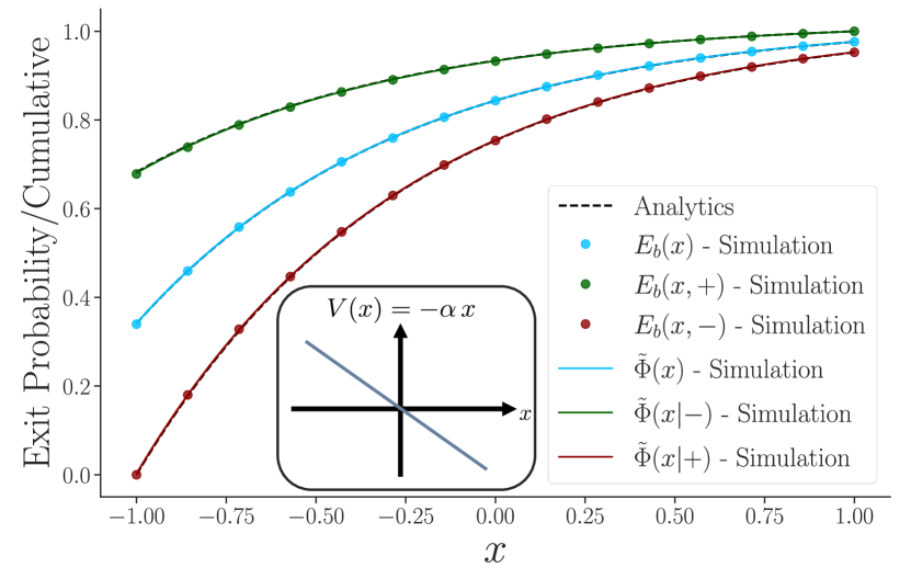
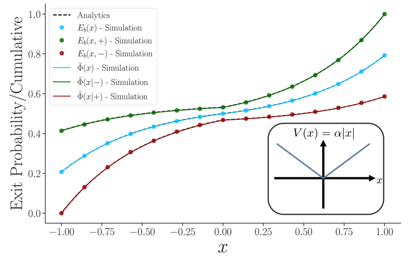
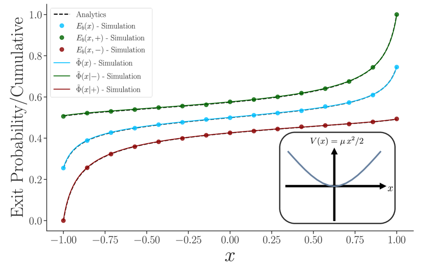
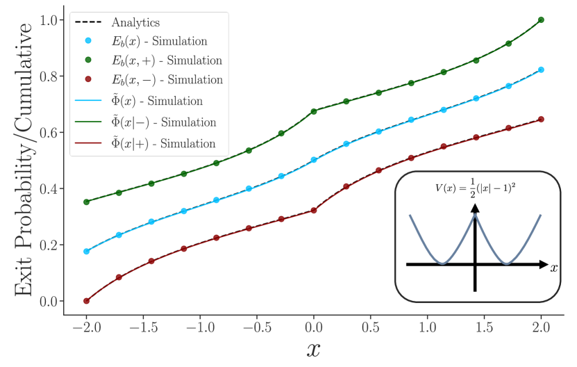
Figure 2: This figure illustrates the duality relations $E_{b}(x)=\tilde{\Phi}(x)$ (48) and $E_{b}(x,\pm)=\tilde{\Phi}(x|\mp)$ (49) for a run-and-tumble particle (RTP). We compute the exit probability (resp. the cumulative distribution) of a RTP in various external potentials $V(x)$ (resp. $-V(x)$), with absorbing walls (resp. hard walls) located at positions $x=a$ and $x=b$. The solid lines show numerical simulations of the cumulative $\tilde{\Phi}$ while the dots are obtained from simulations of the exit probability $E_{b}$. The data from $E_{b}$ and $\tilde{\Phi}$ overlap exactly. Explicit analytical solutions (dotted lines) are also plotted in dashed line. Throughout this analysis, we ensure that the condition $|F(x)|<v_{0}$ is satisfied. Top left: $V(x)=-\alpha\,x$, $\gamma=1$, $\alpha=0.5$, $v_{0}=1$, $a=-1$, $b=1$. Top right: $V(x)=\alpha|x|$, $\gamma=1$, $\alpha=0.6$, $v_{0}=1$, $a=-1$, $b=1$. Bottom left: $V(x)=\mu\,x^{2}/2$, $\gamma=1$, $\mu=1.9$, $v_{0}=2$, $a=-1$, $b=1$. Bottom right: $V(x)=1/2\,(|x|-1)^{2}$, $\gamma=1$, $v_{0}=2$, $a=-2$, $b=2$.

5 Duality relation for a run-and-tumble particle in the stationary state

Let us write the dual $y(t)$ of the process $x(t)$ defined in Eq. (11), as introduced in (3),

$$\dot{y}(t)=-F(y)+v_{0}\,\tilde{\sigma}(t)\,,$$ (47)

where $\tilde{\sigma}(t)$ is a different realisation of the same telegraphic noise defined in Eq. (12). The process $y(t)$ describes the motion of a run-and-tumble particle subjected to the reversed force $-F(y)$. We denote by $\tilde{\Phi}(y)$ the cumulative of the dual process. From Eq. (43), we observe that one can link the exit probability of an RTP (22) to the cumulative of its dual via the following relation

$$E_{b}(x)=\tilde{\Phi}(x)\,,$$ (48)

which is the specialisation of (9) to the RTP case in the stationary state. One can also write a more general relation for the two states of the RTP relating Eq. (23) to Eq. (46),

$$E_{b}(x,\pm)=\tilde{\Phi}(x|\mp)\,,$$ (49)

which is in fact (6) written for an RTP. Note that the derivation of the exit probability is simpler than the one of the cumulative, in particular because the boundary conditions for the density are more subtle. In Figure 2, we check numerically these relations for different forces $F(x)$ such that $|F(x)|<v_{0}$.

Let us stress an important consequence of this relation, which is specific to active particles (in the absence of diffusion). On the one hand, an RTP with initial position at $x=a^{+}$ can still go away from the wall and eventually exit at $x=b$ as long as its velocity is positive at early times, and thus $E_{b}(a^{+},+)$ is generally non-zero (and similarly $E_{b}(b^{-},-)<1$). On the other hand, active particles tend to accumulate near hard walls, leading to delta peaks in the stationary density at $x=a$ and $x=b$ (where the RTP is in the $-$ and $+$ state respectively), such that $\Phi(a^{+},-)>0$ and $\Phi(b^{-},+)<1$. The identity (49) shows that this two phenomena are related, since $E_{b}(a^{+},+)=\tilde{\Phi}(a^{+},-)$ and $E_{b}(b^{-},-)=\tilde{\Phi}(b^{-},+)$ (see Fig. 2).

In Section 6, we comment on what can happen for a general force in the presence of turning points $F(x)=\pm v_{0}$. In this general case, the stationary distribution may depend on the initial condition (since part of the space may be inaccessible to the particle), and therefore it is important that the dual starts its motion at the wall $y=b$ (see [55]).

6 Comments on the exit probability of an RTP subjected to a general force

Here we present an extension of the results of Section 5 to encompass a broader range of forces that do not satisfy the condition $|F(x)|<v_{0}$. This extension allows for forces with multiple turning points, i.e. points such that $F(x)=\pm v_{0}$, within the interval $[a,b]$, as well as regions where the force either falls below $-v_{0}$ or exceeds $v_{0}$ for certain values of $x$ in the same interval (see [24] where a similar situation is considered for the stationary distribution of an RTP). We begin by examining the exit probability for a RTP described by the process $x(t)$ defined in (11). There are two absorbing walls located at $x=a$ and $x=b$. To do so, we introduce the following definition:

$$x_{-}=\ {\rm sup}\left(\{x\in[a,b]\ |\ F(x)\leq-v_{0}\}\cup\{a\}\right)\;.$$ (50)

Both states of the RTP have negative (or null) velocity at $x_{-}$ implying that $E_{b}(x\in[a,x_{-}]|\pm)=0$. Consequently, if the particle initiates its motion inside $]x_{-},b]$ and reaches the position $x_{-}$, it will remain within the interval $[a,x_{-}]$ at all subsequent times. Naturally, it will be unable to exit at $x=b$. As a result, in terms of the exit probabilities (at infinite time) $E_{b}(x,\pm)$, the system behaves as if there were an absorbing wall positioned at $x_{-}$. Let us now define

$$x_{+}=\ {\rm inf}\left(\{x\in[x_{-},b]\ |\ F(x)\geq v_{0}\}\cup\{b\}\right)\;.$$ (51)

At the position $x_{+}$, $\pm$ states of the RTP have a positive (or null) speed, and we also have $F(x)>-v_{0}$ for all $x\in[x_{+},b]$. Hence, if the particle reaches $x_{+}$ from its left, it is guaranteed to eventually exit at $x=b$ so that $E_{b}(x\in[x^{+},b])=1$. Therefore, if we are only interested in the exit probability at infinite time, we can consider that the absorbing wall at $x=b$ is actually replaced by an effective one at $x_{+}$. For an illustration, see the left panel of Figure (3).

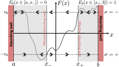
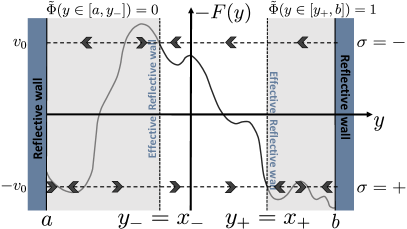
Figure 3: We show here an illustration of the statements of Section 6 which aim to generalize results from Section 5 for a force $F(x)$ that can take any value in $\mathbb{R}$. We are interested in the calculation of the exit probability of an RTP (right panel), and in the cumulative distribution of its dual (left panel). We represent the velocity of the negative state of the RTP on the top dotted line, while the velocity of the positive state is shown on the bottom dotted lines of the plots. If the velocity of the particle is positive, the arrow points to positive values of the abscissa, while if it is negative, it points to the opposite.

Now, let us consider the dual process $y(t)$ defined in (47). At $t=0$, the dual process begins at position $y=b$, and there are two hard walls at $a$ and $b$. As mentioned earlier, unlike the case where $|F(y)|<v_{0}$ holds everywhere, the stationary state of this dual process will depend on its initial condition. In this context, we introduce the following definition

$$y_{-}=\ {\rm sup}\left(\{y\in[a,b]\ |\ -F(y)\geq v_{0}\}\cup\{a\}\right)\;.$$ (52)

At position $y_{-}$, the negative state of the dual RTP has zero speed, while the positive state has a positive velocity. Consequently, as the particle starts its motion at $y=b$, it will always remain at positions such that $y\geq y_{-}$. In particular, this leads to $\tilde{\Phi}(y\in[a,y_{-}])=0$. Therefore, introducing a hard wall at $y_{-}$ will not change the stationary distribution of positions. Similarly, we define

$$y_{+}=\ {\rm inf}\left(\{y\in[y_{-},b]\ |\ -F(y)\leq-v_{0}\}\cup\{b\}\right)\;.$$ (53)

At position $y_{+}$, the negative state of the particle has a negative speed, while the positive state has zero speed. Furthermore, for all $y\in[y_{+},b]$, we have $-F(y)<v_{0}$ and thus, in a finite amount of time, the particle that started at $b$ will reach $y_{+}$. Consequently, we will have $\tilde{\Phi}(y\in[y_{+},b])=1$. Therefore, if our objective is solely to determine the stationary distribution of the dual process, we can assume the existence of a hard wall at $y_{+}$.

At this point, it becomes clear that the definitions of $x_{-}$ and $x_{+}$ coincides with the one of $y_{-}$ and $y_{+}$. In Figure 3, we provide an illustration of these statements. One can then apply the results of Section 3 and Section 4 on the interval $(x_{-},x_{+})$ replacing $a$ with $x_{-}+\epsilon$ and $b$ with $x_{+}-\epsilon$ and taking $\epsilon\to 0$ (some integrals diverge in this limit, but the divergences compensate leading to a well-defined finite limit). When $x_{-}$ or $x_{+}$ is strictly inside $(a,b)$, there is no discontinuity of $E_{b}$ and $\tilde{\Phi}$ at this point. For the exit probability this is because a particle at $x_{-}+\epsilon$ will have zero total velocity if it is in the $+$ state (since $F(x_{-})=-v_{0}$), and thus it will not be able to escape, leading to $E_{b}(x_{-}+\epsilon,+)=0$ (and similarly $E_{b}(x_{+}-\epsilon,-)=1$). For the stationary distribution, this is because it requires an infinite time for the particle to reach the walls (since for instance $-F(x_{-})=v_{0}$), and thus there is no delta peak at the walls (hence $\tilde{\Phi}(x_{-}+\epsilon|-)=0$ and $\tilde{\Phi}(x_{+}-\epsilon|+)=1$). In both cases it is as if the particle inside the interval $(x_{-},x_{+})$ does not “feel” the presence of the walls. For the stationary density, one thus recovers the results of [22].

It is important to note that, in the scenario where turning points are present, we do not necessarily have $E_{a}(x,\pm)=1-E_{b}(x,\pm)$. However, a similar reasoning can be made to obtain the exit probability at $a$. In this case, we define:

$$\begin{split}&x_{+}=\ {\rm inf}\left(\{x\in[a,b]\ |\ F(x)\geq v_{0}\}\cup\{b\}\right)\;,\\ &x_{-}=\ {\rm sup}\left(\{x\in[a,x_{+}]\ |\ F(x)\leq-v_{0}\}\cup\{a\}\right)\;,\end{split}$$ (54)

or similarly for $y_{-}$ and $y_{+}$.

As a conclusion, all the duality results of Section 5 remain true if there are points such that $|F(x)|>v_{0}$, although one has to be more careful when computing both $E_{b}$ and $\tilde{\Phi}$.

7 Conclusion

We have introduced a duality relation for active particle models connecting the exit probability with the cumulative distribution of the position in the presence of hard walls. In the case of an RTP in the stationary state, we obtained explicit expressions for both quantities, which enabled us to illustrate this relation with a concrete example. In a future work [55], we will show how to derive this relation in a much more general setting, that encompasses not only the most studied models of active particles, but also other stochastic processes which are of interest in physics. We hope this result will open the way for new results concerning in particular the first passage properties of active particles, from analytical, numerical as well as experimental viewpoints.

Acknowledgments

We thank P. Le Doussal, S. N. Majumdar and G. Schehr for useful comments and discussions. We also thank J. Klinger and B. De Bruyne for interesting discussions in the early stage of the project.

Appendix

Appendix A Explicit formulas for the exit probabilities of an RTP inside a linear potential and a double-well potential

Linear potential: The linear potential $V(x)=\alpha\,|x|$ leads to a force $F(x)=-\alpha\,\text{sign}(x)$. This force is constant up to the sign of $x$. To have $|F(x)|<v_{0}$ in $[a,b]$, we impose $|\alpha|<v_{0}$. We also fix the location of the walls: $a=-1$, and $b=1$. For positive values of $x$, i.e. $0\leq x\leq 1$, one has

$$E_{b}(x,\pm)=\frac{1}{Z}\left[1\pm e^{\frac{2\gamma\alpha(x-1)}{v_{0}^{2}-\alpha^{2}}}+\frac{v_{0}}{\alpha}\left(1-2e^{-\frac{2\gamma\alpha}{v_{0}^{2}-\alpha^{2}}}+e^{\frac{2\gamma\alpha(x-1)}{v_{0}^{2}-\alpha^{2}}}\right)\right]\,,$$ (55)

while for negative values of $x$, i.e. $-1\leq x\leq 0$, one has

$$E_{b}(x,\pm)=\frac{1}{Z}\left[1\pm e^{-\frac{2\gamma\alpha(1+x)}{v_{0}^{2}-\alpha^{2}}}+\frac{v_{0}}{\alpha}\left(1-e^{-\frac{2\gamma\alpha(1+x)}{v_{0}^{2}-\alpha^{2}}}\right)\right]\,.$$ (56)

The normalisation constant reads

$$Z=2\left[1+\frac{v_{0}}{\alpha}\left(1-e^{-\frac{2\gamma\alpha}{v_{0}^{2}-\alpha^{2}}}\right)\right]\,.$$ (57)

Double-well potential: In this scenario, we examine a potential described by $V(x)=\frac{\mu}{2}\left(|x|-x_{0}\right)^{2}$, which gives rise to a force $F(x)=\mu(x_{0}-|x|)\,\text{sign}(x)$. We constrain the location of the walls such that $b<1+v_{0}$ and $a>-1-v_{0}$ in order to have $|F(x)|<v_{0}$ in $[a,b]$. For positive values of $x$, the exit probabilities are given by (here we fix $x_{0}=1$ and $\mu=1$ to simplify the expressions)

$$E_{b}(x,\pm)=\frac{1}{Z}\left\{1\pm\left(\frac{(1+a)^{2}-v_{0}^{2}}{v_{0}^{2}-(x-1)^{2}}\right)^{\gamma}+\frac{2\gamma}{v_{0}}\,\left(1-\frac{(1+a)^{2}}{v_{0}^{2}}\right)^{\gamma}\left[2\,_{2}F_{1}\left(\frac{1}{2},1+\gamma,\frac{3}{2},\frac{1}{v_{0}^{2}}\right)\right.\right.$$

$$\left.\left.-(1+a)\,_{2}F_{1}\left(\frac{1}{2},1+\gamma,\frac{3}{2},\frac{(1+a)^{2}}{v_{0}^{2}}\right)+(x-1)\,_{2}F_{1}\left(\frac{1}{2},1+\gamma,\frac{3}{2},\frac{(x-1)^{2}}{v_{0}^{2}}\right)\right]\right\}\,.$$ (58)

For negative values of $x$, they read

$$E_{b}(x,\pm)=\frac{1}{Z}\left\{1\pm\left(\frac{(1+a)^{2}-v_{0}^{2}}{(1+x)^{2}-v_{0}^{2}}\right)^{\gamma}+\frac{2\gamma}{v_{0}}\,\left(1-\frac{(1+a)^{2}}{v_{0}^{2}}\right)^{\gamma}\right.$$

$$\left.\times\left[(1+x)\,_{2}F_{1}\left(\frac{1}{2},1+\gamma,\frac{3}{2},\frac{(1+x)^{2}}{v_{0}^{2}}\right)-(1+a)\,_{2}F_{1}\left(\frac{1}{2},1+\gamma,\frac{3}{2},\frac{(1+a)^{2}}{v_{0}^{2}}\right)\right]\right\}\,.$$ (59)

The normalisation is

$$Z=1+\left(\frac{(1+a)^{2}-v_{0}^{2}}{(1-b)^{2}-v_{0}^{2}}\right)^{\gamma}+\frac{2\gamma}{v_{0}}\,\left(1-\frac{(1+a)^{2}}{v_{0}^{2}}\right)^{\gamma}\left[2\,_{2}F_{1}\left(\frac{1}{2},1+\gamma,\frac{3}{2},\frac{1}{v_{0}^{2}}\right)\right.\quad\quad\quad$$

$$\left.-(1+a)\,_{2}F_{1}\left(\frac{1}{2},1+\gamma,\frac{3}{2},\frac{(1+a)^{2}}{v_{0}^{2}}\right)+(b-1)\,_{2}F_{1}\left(\frac{1}{2},1+\gamma,\frac{3}{2},\frac{(b-1)^{2}}{v_{0}^{2}}\right)\right]\,.$$ (60)

References

References

- [1] M. C. Marchetti, J. F. Joanny, S. Ramaswamy, T. B. Liverpool, J. Prost, M. Rao, R. Aditi Simha, Hydrodynamics of soft active matter, Rev. Mod. Phys. 85, 3 1143–1189 (2013).
- [2] C. Bechinger, R. Di Leonardo, H. Löwen, C. Reichhardt, G. Volpe, G. Volpe, Active particles in complex and crowded environments, Rev. Mod. Phys. 88, 4 045006 (2016).
- [3] S. Ramaswamy, Active matter, J. Stat. Mech. 054002 (2017).
- [4] E. Fodor, M. Cristina Marchetti, The statistical physics of active matter: From self-catalytic colloids to living cells, Physica A: Statistical Mechanics and its Applications 504 106-120 (2018).
- [5] P. Romanczuk, M. Bär, W. Ebeling, B. Lindner, and L. Schimansky-Geier, Active Brownian particles, Eur. Phys. J. Spec. Top. 202, 1-162 (2012).
- [6] D. Martin, J. O’Byrne, M. E. Cates, E. Fodor, C. Nardini, J. Tailleur, F. van Wijland, Statistical mechanics of active Ornstein-Uhlenbeck particles, Phys. Rev. E 103, 032607 (2021).
- [7] L. L. Bonilla, Active Ornstein-Uhlenbeck particles, Phys. Rev. E 100, 022601 (2019).
- [8] U. Basu, S. N. Majumdar, A. Rosso, and G. Schehr, Active Brownian motion in two dimensions, Phys. Rev. E, 98(6), 062121 (2018).
- [9] J. Tailleur, M. E. Cates, Statistical mechanics of interacting run-and-tumble bacteria, Phys. Rev. Lett. 100, 218103 (2008).
- [10] M. E. Cates, Diffusive transport without detailed balance: Does microbiology need statistical physics?, Rep. Prog. Phys. 75, 042601 (2012).
- [11] M. Kac, A stochastic model related to the telegrapher’s equation, Rocky Mountain J. Math. 4, 497 (1974).
- [12] E. Orsingher, Random motions governed by third-order equations, Stoch. Process. Their Appl. 34, 49 (1990)
- [13] G. H. Weiss, Some applications of persistent random walks and the telegrapher’s equation, Physica A 311, 381-410 (2002).
- [14] H. C. Berg, E. Coli in Motion, (Springer Verlag, Heidelberg, Germany) (2004).
- [15] C. F. Lee, Active particles under confinement: aggregation at the wall and gradient formation inside a channel, New J. Phys. 15 055007 (2013).
- [16] X. Yang, M. L. Manning and M. C. Marchetti, Aggregation and segregation of confined active particles, Soft Matter, 10, 6477 (2014).
- [17] W. E. Uspal, M. N. Popescu, S. Dietrich and M. Tasinkevych, Self-propulsion of a catalytically active particle near a planar wall: from reflection to sliding and hovering, Soft Matter 11, 434 (2015).
- [18] A. Duzgun and J. V. Selinger, Active Brownian particles near straight or curved walls: Pressure and boundary layers, Phys. Rev. E 97, 032606 (2018).
- [19] L. Angelani, Confined run-and-tumble swimmers in one dimension, J. Phys. A: Math. Theor. 50, 325601 (2017).
- [20] C. Sandford, A. Y. Grosberg, and J.-F. Joanny, Pressure and flow of exponentially self-correlated active particles, Phys. Rev. E 96, 052605 (2017).
- [21] L. Caprini and U. M. B. Marconi, Active particles under confinement and effective force generation among surfaces, Soft matter 14, 9044-9054 (2018).
- [22] A. Dhar, A. Kundu, S. N. Majumdar, S. Sabhapandit and G. Schehr, Run-and-tumble particle in one-dimensional confining potentials, Phys. Rev. E 99, 032132 (2019).
- [23] F. J. Sevilla, A. V. Arzola, and E. P. Cital,Stationary superstatistics distributions of trapped run-and-tumble particles, Phys. Rev. E 99, 012145 (2019).
- [24] P. Le Doussal, S. N. Majumdar and G. Schehr, Velocity and diffusion constant of an active particle in a one-dimensional force field, EPL 130 40002 (2020).
- [25] S. Redner, A guide to first-passage processes, Cambridge university press, (2001).
- [26] R. Metzler, S. Redner and G. Oshanin, First-passage phenomena and their applications, Vol. 35, World Scientific, (2014).
- [27] A. J. Bray, S. N. Majumdar and G. Schehr, Persistence and first-passage properties in nonequilibrium systems, Adv. Phys. 62, 225 (2013).
- [28] O. Bénichou, C. Loverdo, M. Moreau, and R. Voituriez, Intermittent search strategies Reviews of Modern Physics, 83(1), 81. (2011).
- [29] O. Bénichou, M. Coppey, M. Moreau, P. H. Suet, and R. Voituriez, Optimal search strategies for hidden targets, Phys. Rev. Lett. 94(19), 198101 (2005).
- [30] U. Basu, S. Sabhapandit, and I. Santra, Target search by active particles, arXiv:2311.17854 (2023).
- [31] P. Hanggi, and P. Jung, Colored Noise in Dynamical Systems, Adv. Chem. Phys. 89, 239 (1995).
- [32] K. Malakar, V. Jemseena, A. Kundu, K. Vijay Kumar, S. Sabhapandit, S. N. Majumdar, S. Redner, A. Dhar, Steady state, relaxation and first-passage properties of a run-and-tumble particle in one-dimension, Phys. Rev. E 103, 032607 (2021)
- [33] B. De Bruyne, S. N. Majumdar and G. Schehr, Survival probability of a run-and-tumble particle in the presence of a drift, J. Stat. Mech. (2021) 043211.
- [34] P. Singh, S. Sabhapandit and A. Kundu, Run-and-tumble particle in inhomogeneous media in one dimension, J. Stat. Mech. (2020) 083207.
- [35] P. Singh, S. Santra and A. Kundu, Extremal statistics of a one-dimensional run and tumble particle with an absorbing wall, J. Phys. A: Math. Theor. 55 465004 (2022).
- [36] S. A. Iyaniwura and Z. Peng, Asymptotic analysis and simulation of mean first passage time for active Brownian particles in 1-D, arXiv:2310.04446 (2023).
- [37] M. Guéneau, S. N. Majumdar and G. Schehr, Optimal mean first-passage time of a run-and-tumble particle in a one-dimensional confining potential, arXiv:2311.06923 (2023).
- [38] L. Angelani, One-dimensional run-and-tumble motions with generic boundary conditions, J. Phys. A: Math. Theor. 56 455003 (2023).
- [39] P. C. Bressloff, Encounter-based model of a run-and-tumble particle II: absorption at sticky boundaries, J. Stat. Mech. (2023) 043208.
- [40] E. Jeon, B. Go and Y. W. Kim, Searching for a partially absorbing target by a run-and-tumble particle in a confined space, arxiv-2310.04016 (2023).
- [41] V. Tejedor, R. Voituriez, and O. Bénichou, Optimizing persistent random searches, Phys. Rev. Lett. 108, 088103 (2012).
- [42] J.-F. Rupprecht, O. Bénichou, and R. Voituriez, Optimal search strategies of run-and-tumble walks, Phys. Rev. E 94, 012117 (2016).
- [43] F. Mori, P. Le Doussal, S. N. Majumdar and G. Schehr, Universal Survival Probability for a d-Dimensional Run-and-Tumble Particle, Phys. Rev. Lett. 124, 090603 (2020).
- [44] C. W. Gardiner, Handbook of stochastic methods, Berlin : springer (1985).
- [45] S. N. Majumdar, A. Rosso, A. Zoia, Hitting probability for anomalous diffusion processes, Phys. Rev. Lett. 104, 020602 (2010).
- [46] P. Lévy, Processus stochastiques et mouvement brownien, Gauthier-Villars, Paris (1948).
- [47] D. Lindley, The theory of queues with a single server, Mathematical Proceedings of the Cambridge Philosophical Society 48(2), 277-289 (1952).
- [48] D. Siegmund, The Equivalence of Absorbing and Reflecting Barrier Problems for Stochastically Monotone Markov Processes, Ann. Probab. 4(6): 914-924 (1976).
- [49] S. Asmussen and K. Sigman, Monotone Stochastic Recursions and their Duals, Probability in the Engineering and Informational Sciences 10(1), 1-20 (1996).
- [50] K. Sigman and R. Ryan, Continuous-time monotone stochastic recursions and duality, Advances in Applied Probability 32(2), 426-445 (2000).
- [51] M. V. Chubynsky and G. W. Slater, Diffusing Diffusivity: A Model for Anomalous, yet Brownian, Diffusion, Phys. Rev. Lett. 113, 098302 (2014).
- [52] V. Sposini, A. Chechkin and R. Metzler, First passage statistics for diffusing diffusivity, J. Phys. A: Math. Theor. 52, 04 (2019).
- [53] M. R. Evans, and S. N. Majumdar, Diffusion with stochastic resetting, Phys. Rev. Lett. 106(16), 160601 (2011).
- [54] M. R. Evans, S. N. Majumdar and G. Schehr, Stochastic resetting and applications, J. Phys. A: Math. Theor. 53, 193001 (2020).
- [55] M. Guéneau and L. Touzo, to be published.
- [56] V. Sposini, R. Metzler and G. Oshanin, Single-trajectory spectral analysis of scaled Brownian motion, New J. Phys. 21, 073043 (2019).