An improved Halo Occupation Distribution prescription from UNITsim H_α emitters: conformity and modified radial profile

Abstract

The Euclid mission is poised to make unprecedented measurements in cosmology from the distribution of galaxies with strong H_α spectral emission lines. Accurately interpreting this data requires understanding the imprints imposed by the physics of galaxy formation and evolution on galaxy clustering. In this work we utilize a semi-analytical model of galaxy formation (SAGE) to explore the necessary components for accurately reproducing the clustering of Euclid-like samples of H_α emitters. We focus on developing a Halo Occupation Distribution (HOD) prescription able to reproduce the clustering of SAGE galaxies. Typically, HOD models assume that satellite and central galaxies of a given type are independent events. We investigate the need for conformity, i.e. whether the average satellite occupation depends on the existence of a central galaxy of a given type. Incorporating conformity into HOD models is crucial for reproducing the clustering in the reference galaxy sample. Another aspect we investigate is the radial distribution of satellite galaxies within haloes. The traditional density profile models, NFW and Einasto profiles, fail to accurately replicate the small-scale clustering measured for SAGE satellite galaxies. To overcome this limitation, we propose a generalization of the NFW profile, thereby enhancing our understanding of galaxy clustering.

1 INTRODUCTION

The study of the large-scale structure in the Universe plays a crucial role in contemporary cosmology. It serves as a powerful tool for understanding the fundamental properties of our Universe, including the values of different cosmological parameters and the nature of dark matter and dark energy. Galaxy clustering is an observable that allows us to probe both the cosmological parameters and the physics of galaxy formation.

Over the past few decades, numerous endeavours have been dedicated to creating large galaxy maps, such as the 2dFGRS (Cole et al., 2005), SDSS (York et al., 2000; Eisenstein et al., 2005), WiggleZ (Drinkwater et al., 2010; Parkinson et al., 2012), BOSS (Dawson et al., 2013; Alam et al., 2017), eBOSS (Dawson et al., 2016; Alam et al., 2021a), and DES (The Dark Energy Survey Collaboration, 2005; Abbott et al., 2018). These endeavors have enhanced our understanding of the Universe, by providing measurements of its expansion history and increasing the constrains on dark energy and alternative theories of gravity. These cosmological surveys have provided the community with large 3-D maps of galaxies up to $z\sim 1$, allowing for a better understanding of the evolution of galaxies. Despite significant progress, these areas of investigation remain open and ongoing.

New generation surveys, including Euclid (Laureijs et al., 2011; Amendola et al., 2018), DESI (DESI Collaboration et al., 2016), the Nancy Grace Roman Space Telescope (Spergel et al., 2013, 2015) and the 4-metre Multi-Object Spectroscopic Telescope (de Jong et al., 2012), are set to map galaxies beyond $z\sim 1$ and to increase the density of QSOs at higher redshifts. One of the main tracers beyond $z\sim 1$ are galaxies with strong spectral emission lines or emission line galaxies (ELGs). In particular, Euclid utilizes near-infrared grisms to observe galaxies with a strong H_α spectral line, or H_α emitters.

H_α emitters are mostly galaxies with strong star formation rates (e.g. Favole et al., 2023). From both hydrodynamical and semi-analytical models (SAMs) of galaxy formation, we expect the connection between galaxies selected by their star-formation rate and dark matter haloes to be more complex than for stellar-mass selected samples (e.g. Zheng et al., 2005; Orsi & Angulo, 2018; Gonzalez-Perez et al., 2020). SAMs of galaxy formation and evolution populate dark matter haloes at early cosmic times with gas and let them evolve with a set of coupled differential equations (e.g. Cole et al., 2000; Croton et al., 2016; Hirschmann et al., 2016; Cora et al., 2018; Lagos et al., 2019). These equations aim to encapsulate the physical processes that are understood to be relevant during the formation and evolution of galaxies, such as the cooling of gas, the formation of stars, the interplay between super massive black holes and the intergalactic medium, etc (see the reviews on modelling galaxies by Baugh, 2006; Somerville & Davé, 2015; Wechsler & Tinker, 2018). SAMs are faster than hydrodynamical simulations (e.g. Schaye et al., 2015; McCarthy et al., 2017; Springel et al., 2018; Pillepich et al., 2018), as they are ran on dark matter only N-body simulations, at the expense of loosing the effect that baryons have over dark matter haloes (Schneider & Teyssier, 2015; Aricò et al., 2020).

In this work we use SAGE, the SAM introduced in Croton et al. (2016), to explore how H_α emitters populate dark matter halos. SAMs have been previously used to produce Euclid-like and Roman-like H_α emitter catalogues that have been used to understand the clustering of H_α galaxies and their relation to halos  (Merson et al., 2018; Zhai et al., 2019, 2021b, 2021a; Knebe et al., 2022). Here we use the SAGE run on the UNIT dark-matter only simulation (Chuang et al., 2019), as described and released in the work by Knebe et al. (2022). This simulation uses the fixed and paired technique to increase its effective volume, allowing more precise statistical analyses (Angulo & Pontzen, 2016).

SAMs can produce model galaxies accounting for a large range of physical phenomena in simulation volumes comparable to those required to interpret observations from current cosmological surveys. Nevertheless, they are still too slow to be able to produce many realisations and they require the construction of merger trees tracing the evolution of halos in fine time slices, which is not available in many simulations due to computing/storing limitations. The Halo Occupation Distribution (HOD) model provides a simplified way to describe the relation between galaxies and haloes and can be constructed from a single halo catalogue. These simplifications makes HOD valid for the target observables they are constructed to match, but sometimes will show limitations when trying to extend it to other observables  (e.g. Chaves-Montero et al., 2023).

HOD models are computationally efficient. They have demonstrated their capability to reproduce the observed clustering across a range of galaxies, including the dependency with luminosity and colour (Zehavi et al., 2005; Christodoulou et al., 2012; Carretero et al., 2015). In their basic form, HOD models assume that the mass of haloes determine the average number of galaxies thy can host (e.g. Benson et al., 2000; Berlind et al., 2003; Zheng et al., 2005). Catalogues of model galaxies produced with HOD models can be produced fast enough as to choose the best fit to a set of clustering observables using statistical techniques that require hundreds or thousands of realisations in large simulation volumes (e.g. Alam et al., 2021b; Yuan et al., 2023a; Rocher et al., 2023a). HOD models have become a popular tool for producing realistic mock catalogs in large simulation volumes to match the clustering of a target galaxy sample (e.g., in BOSS, DES and eBOSS: Manera et al., 2013; Avila et al., 2018, 2020).

The objective of this work is to construct an HOD model that accurately reproduces the galaxy clustering of the Euclid H_α emitters modelled by SAGE. In particular, we explore if two of the usual assumptions made by HOD models should be challenged when compared with model H_α emitters. One of this usual assumptions is that central and satellite galaxies of a certain type are independent events within a halo, a lack of conformity. The other is the modelling of the radial profile of satellite galaxies.

One of the main focus of this paper is to study the effect that galactic conformity has on the clustering of H_α emitters. The term galactic conformity was first coined by Weinmann et al. (2006) to describe strong correlations between the properties of satellite galaxies and their central galaxies in data from the Sloan Digital Sky Survey (SDSS). A strong 1-halo conformity for ELGs has recently been suggested from the comparison of DESI data with model galaxies produced with different HOD models (Rocher et al., 2023b; Gao et al., 2023). Overall, galactic conformity remains an active research topic and a significant puzzle in the formation and evolution of galaxies.

The second main focus of this work is to explore whether the typical assumptions made by HOD models for the radial profiles of satellite galaxies are upheld. Commonly, HOD models assume that the distribution of satellite galaxies within the dark matter halo follows the distribution of the dark matter itself, or often an NFW (Navarro et al., 1997) or an Einasto (Einasto, 1969) profile. We will try different ways to sample these types of profiles and also propose an extension.

The plan of this paper is as follows. In section (§ 2) we introduce UNIT DM simulation. In section (§ 3) we describe the model galaxy sample of reference. First (§ 3.1), we introduce UNITsim-SAGE, how our reference H_α galaxy sample for Euclid is built and we describe the average halo occupation distribution that we find. We then describe in (§ 3.2) how we build the final sample of reference by applying the shuffling method to the previous model sample. In section (§ 4), we detail the various halo occupation models and properties that we employ to generate mock catalogues. Section (§ 5) discusses conformity, the method we employ to model it and its effect in galaxy clustering. Section (§ 6) is devoted to studying the radial profile of SAGE and how to reproduce it in order to recover accurate H_α galaxy clustering. Finally, in Section (§ 7), we conclude and discuss our findings and future prospects.

2 UNIT DM simulation

The UNIT suite is a set of N-body cosmological simulations (Chuang et al., 2019) designed to cover the expected halo masses for emission line galaxies (ELGs), in particular [OII] emitters targeted by DESI ($\sim 10^{11}h^{-1}{\rm M}_{\odot}$ Gonzalez-Perez et al., 2020) and Euclid H_α emitters ($\sim 4\times 10^{11}h^{-1}{\rm M}_{\odot}$ Cochrane et al., 2017). To reduce the cosmic variance in the UNIT simulations, we employ the Fix and Pair method (Angulo & Pontzen, 2016). Following this method, two pairs of simulations are generated with initial conditions with a power spectrum with an amplitude fixed to the expected value, given by the input power spectrum. The initial conditions of one of the simulations from each pair is set with the opposite phases than the other one from the pair (Chuang et al., 2019). These simulations were generated using GADGET2 (Springel, 2005), which fully solves the gravitational evolution of the continuous distribution of dark matter. The phase-space halo finder ROCKSTAR (Behroozi et al., 2013a) was used to identify haloes from the $129$ existing snapshots. Subsequently, the ConsistentTrees software (Behroozi et al., 2013a) was employed to calculate their merging histories. The software tracks dark matter halos (regions of the universe where gravity has made matter collapse into denser structures) as they evolve over time and move in space, constructing a tree-structure that illustrates how these halos merge together to form larger halos. These merger trees are ’consistent’ in the sense that the mass and position of a halo at a given moment in the tree are informed by the mass and position of its progenitors and its descendants.

For this work we use simulations with boxes of side $1h^{-1}\text{Gpc}$ and $4096^{3}$ dark matter particles. The cosmological parameters of these simulations are: $\Omega_{m,0}=1-\Omega_{\Lambda,0}=0.3089,\hskip 7.11317pth=0.6774,\hskip 7.11317ptn_{\rm s}=0.9667,\hskip 7.11317pt\sigma_{8}=0.8147$.

We perform our analysis over the simulation snapshot at $z=1.321$, which approximately corresponds to the mean redshift expected for Euclid H_α emitters, $0.9<z<1.8$.

3 UNITsim-sage: Reference galaxy sample

We aim to provide an improved Halo Occupation Distribution model for Euclid-like H_α emitters, focusing on conformity and satellite radial profiles. Our reference catalogue of galaxies is generated from the UNITsim-Galaxies catalogues described in Knebe et al. (2022) and released along it . This catalogue is based on the SAGE semi-analytical model of galaxy formation and evolution (Croton et al., 2016) by populating the dark-matter-only UNITsim simulations (section 2). For each model galaxy, spectral emission lines associated with star formation events are obtained with the get_emlines model described in Orsi et al. (2014). One of these spectral lines is the H_α, targeted by Euclid. The spectral emission lines are then attenuated by dust using a Cardelli et al. (1989) law following the code developed in Favole et al. (2020). All these models were implemented in the catalogue in Knebe et al. (2022) and we refer the reader to that publication for a more detailed description.

In order to single out the modelling of both conformity and the satellite radial profiles, we use a shuffled sample, SAGE_sh (§ 3.2). To construct this sample, we remove the galaxy assembly bias: the effect that other properties beyond halo mass have on the distribution of galaxies within haloes.

3.1 Model H_α emitters with an Euclid-like number density

Sample	$\frac{d^{2}N(z)}{dzdA}$	Number density	Flux cutoff
	$\rm Galaxies\hskip 2.84526ptdeg^{-2}$	$\rm Mpc^{-3}h^{3}$	$\rm ergs\rm s^{-1}\rm cm^{-2}$
Pozzetti nº1	$4377$	$1.299\times 10^{-3}$	$1.041\times 10^{-16}$
Pozzetti nº3	$\mathbf{2268}$	$\mathbf{6.731\times 10^{-4}}$	$\mathbf{1.325\times 10^{-16}}$
Euclid flux	$580.7$	$1.723\times 10^{-4}$	$2\times 10^{-16}$

Table 1: Properties of the three model galaxy catalogues described in section 3. The first column on the left shows the name given to the samples. In the second column we quote the galaxies per square degree per redshift interval from Pozzetti et al. (2016) for the first two samples and the one we obtain applying the H_α flux Euclid-expected limit to the SAGE sample. The third column contains the corresponding numerical volume densities ($n$). The fourth column shows the H_α flux limit needed to recover the target $n$ for the Pozzetti et al. models and the flux limit expected for Euclid. Our reference model from subsection 3.2 onwards is Pozzetti nº3 (or the shuffled version of it, see subsection 3.2 ), which will be referred to as SAGE (or SAGE_sh, when shuffled).

In order to produce Euclid-like catalogues of H_α emitters, we aim to reproduce the mean number density forecasted by Pozzetti et al. (2016) over the entire redshift range observed by Euclid: $0.9<z<1.8$. For this, we use a simulation snapshot at $z=1.321$, which approximately corresponds to the average redshift of Euclid’s targetted redshift range. This approach is slightly different to the one taken in Knebe et al. (2022), where we matched the Pozzetti et al. (2016) differential luminosity function, at the redshift of the snapshot.

Pozzetti et al. (2016) provides a range of forecasts, with the extreme number densities being $n_{1}=1.299\times 10^{-3}$ $\rm Mpc^{-3}h^{3}$ and $n_{3}=6.731\times 10^{-4}$ $\rm Mpc^{-3}h^{3}$, which are tabulated in the first column of Table 1. These volume number densities, $n$, are obtained from the angular ones, $\eta=\frac{d^{2}N(z)}{dzdA}$, provided by Pozzetti et al. (2016) (third column in Table 1), as follows:

$$n=\frac{\eta\hskip 2.84526pt180^{2}}{\pi^{2}\hskip 2.84526ptD_{\rm c}^{2}(z)\hskip 2.84526pt\frac{{\rm d}D_{\rm c}(z)}{{\rm d}z}}\,,$$ (1)

where $D_{\rm c}(z)$ is the comoving distance to the object at redshift $z$. We apply the flux cuts indicated in Table 1 to get the extreme number densities forcasted by Pozzetti et al.. These are well below $2\times 10^{-16}{\rm ergs\,s^{-1}\,cm}^{-2}$, the expected H_α flux limit for Euclid. If we apply this cut to the UNITsim-Galaxies catalogue, we obtain a sample with a number density $1.723\times 10^{-4}$ $\rm{Mpc^{-3}}$$h^{3}$, far below those from Pozzetti et al.’s models. The exact shape of the SAGE H_α luminosity function is very sensitive to the dust attenuation modelling, in particular at the tails of the distribution, sampled by the flux limits. An alternative approach would be to fine tune the dust attenuation model until we match the Pozzetti et al. (2016) luminosity function as done in Zhai et al. (2019). However, this approach is not clear to be more physical than the one taken here, where we are following the approach described in Knebe et al. (2022). A more physical alternative would be to fit simultaneously the dust attenuation parameters, the emission line modelling and the SAM to different available observations with luminosity functions from different lines or even clustering measurements. However, this is beyond the scope of this paper and deserves and stand-alone study.

Figure 1: Top: The mass function of our catalogues of dark matter haloes (dark matter haloes , solid black section 2) and of the different H_α galaxies samples considered: the Euclid-flux raw sample (gold) together with the optimistic (green) and reference (red) samples based on Pozzetti et al. (2016) luminosity functions (see Table 1). The solid curves correspond to the central galaxies and the dashed curves to the satellite galaxies. The mass function corresponds to the density of haloes/galaxies for a given halo mass divided by the halo mass bin size. To achieve this, histograms of objects in the halo/galaxy catalogues are created as a function of $M_{\rm 200c}$, and they are normalized by their volume ($1h^{-1}\text{Gpc}$) and the size of the corresponding log$M_{\rm halo}$ bin. Bottom: the mean halo occupation distribution as a function of halo mass of the haloes. This is compute as the ratio of the galaxy to halo mass functions.

In the upper panel of Figure 1, we present the halo mass function of main dark matter haloes and galaxies for the three samples summarised in Table 1. In this figure, we separate the contributions of central (solid curves) and satellite galaxies (dashed curves). The halo mass functions for dark matter haloes follow a typical shape close to a power law, with a change in the slope at the massive end. Central H_α emitters follow this trend above a mininimum halo mass. The numbers of both central and satellite galaxies decrease rapidly below a minimum halo mass. The number of H_α emitters is lower than that for haloes for all halo masses. As expected, satellite galaxies populate more massive haloes than centrals.

The average halo occupation distribution (HOD) for model H_α emitters selected with different number densities is shown in the lower panel of Figure 1. Satellite H_α emitters follow the typical truncated power law seen for model satellite galaxies (e.g. Zheng et al., 2005; Avila et al., 2022).

The average HOD for central model galaxies do not reach unity, as it would do in a complete sample sample of galaxies without an particular type selection. This was expected from previous theoretical works on star-forming and ELGs (e.g. Zheng et al., 2005; Gonzalez-Perez et al., 2018; Zhai et al., 2021b) and also found for DESI ELGs (Rocher et al., 2023b). This implies that we do not expect to find a H_α emitter in the center of every halo above a certain mass threshold. In Avila et al. (2020), a similar shape for the mean HOD of centrals galaxies, although with a steeper decay, was described as a asymmetric Gaussian.

From this point onward, we use Pozzetti et al.’s Model 3 by default, labelled as SAGE. This model has been used as the baseline for several Euclid studies, as it is expected to be the most realistic.

3.2 SAGE_sh: the shuffled reference galaxy sample

At first order, galaxy clustering at large scales only depends on the mass of the host haloes. However, galaxy clustering can be affected by other halo properties, what is usually known as assembly bias. Assembly bias has been measured from simulated haloes and galaxies in different ways (e.g. Lacerna & Padilla, 2011; Contreras et al., 2021; Jiménez et al., 2021). Moreover, there is compelling observational evidence of galaxy assembly bias (Obuljen et al., 2020; Yuan et al., 2021; Wang et al., 2022; Alam et al., 2023).

Properties encapsulating the environment of haloes have been found to be the most relevant secondary property (e.g. Xu et al., 2021). However, in previous articles, one can observe how other internal properties of the halo, such as $V_{\rm max}$ (which is the maximum circular velocity of the halo) or the haloes own concentration, could explain at least part of the assembly bias. We attempted to construct an HOD prescription based on $V_{\rm max}$ instead of $M_{\rm halo}$ (à la Figure 1) and we found that it reduces the effect of assembly bias signal of SAGE galaxies, but it does not completely eliminate it. The way to quantify the effect was to check the goodness in the recovery of the 2-halo term (large scales) clustering of SAGE (see discussion of Figure 2 below).

This work is focused on the exploration of both conformity and the satellite radial profile. To isolate the effect that varying these properties have on clustering we build a reference galaxy sample for which the effect of assembly bias is removed, SAGE_sh. We can achieve this by shuffling all galaxies within a given halo to the position of another halo of similar mass. This technique was first proposed in Croton et al. (2007). In this proccess, the relative positions (and velocities) of galaxies to the center of a halo as well as internal properties of galaxies are preserved. It is worth noting that the bin size for shuffling coincides with the same binning used to calculate the mean galaxy occupation value (Figure 1). Where the range of the mass is 10.5 < $\rm log_{10}(M_{\rm 200c})$ < 14.5 with a binning of $\Delta$log$M$ = 0.057.

Throughout this paper we quantify the clustering by calculating the real-space two-point correlation function, $\xi$, with the publicly available Cute code (Alonso, 2012) with logarithmic binning, where the number of bins is equal to 80, the bins in r per decade is $8$ and the $r_{\rm max}$ is $140h^{-1}{\rm Mpc}$. The clustering of model Euclid-like H_α emitters before and after the shuffling process is shown in Figure 2. By construction these two agree for the 1-halo term contribution to the clustering (pairs of galaxies within the same halo). From $\sim 0.2{\rm Mpc}/h$, the clustering of the SAGE and SAGE_sh H_α emitters start to differ, and stabilises at larger scales to a difference of about 10 per cent. This difference in the scales dominated by the 2-halo term (pairs of galaxies from different haloes) is due to the history of formation and environments of dark matter haloes, the assembly bias. While for scales smaller than 0.22, the clustering is correctly repopulated, that is, the shuffling does not affect the 1-halo. Note that the shuffling procedure does not alter the two properties we are investigating here, the 1-halo conformity and the distribution of satellite galaxies within haloes as, by construction, the positions and properties of galaxies within haloes are preserved.

In what follows we attempt to reproduce clustering of the shuffled UNITsim-SAGE H_α catalogue, that we label in short SAGE_sh. In Figure 2 we can see our starting point, labeled as Vanilla HOD. In that figure, we can also see the model proposed (default, see subsection 4.3) after the improvements developed in section 5 and section 6. We see that the gain in recovering our reference clustering from SAGE_sh is very remarkable, with our default model closely following the clustering of SAGE_sh. We describe the main properties of these two models in the next section.

Figure 2: Top: Two-point correlation function in real space of different model galaxy catalogues: SAGE (solid orange), shuffled SAGE (SAGE_sh, dashed black) and two HOD catalogues fitted to SAGE. The Vanilla HOD (subsection 4.2, solid blue) uses NFW radial profile and assumes that central and satellite H_α galaxies are independent events (no conformity). The default HOD uses the concept of conformity and the analytical $N(r)$ function implemented for the satellite galaxies fitted to SAGE (subsection 4.3, solid red). Bottom: Ratios with respect to SAGE_sh clustering. The error bars are calculated as the standard deviation of 100 realisations. Remember that we have eliminated the assembly bias, studying Euclid like model galaxies from SAGE_sh, since we decided not to focus on the effects of assembly bias but to analyze other properties.

4 Halo occupation distribution model

In this section we summarise the halo occupation distribution (HOD) model we use to populate with SAGE_sh-like galaxies the UNIT dark matter only simulation.

Halo Occupation Distribution (HOD) models are widely used to assign galaxies of different types to dark matter haloes (e.g. Avila et al., 2020). In their basic form, the mass of the halo determines the average number of galaxies that it hosts (e.g. Benson et al., 2000; Berlind et al., 2003; Zheng et al., 2005). Central and satellite galaxies are modelled separately in HOD models. In order to implement an HOD galaxy assignment prescription, we first need to choose the shape of the mean HOD (§ 4.1.1), then a probability distribution function determines if a halo contains or not a central galaxy and how many satellites (§ 4.1.3). The radial positions (§ 4.1.4) and velocities of satellite galaxies within haloes are chosen next. In this work, we have disregarded the velocities of satellites as our focus is solely on the two-point correlation function statistic in real space.

Throughout this work all the model galaxy catalogues are generated at $z=1.321$ and have fixed number density, $6.731\times 10^{-4}$ $\rm Mpc^{-3}h^{3}$, and linear bias, $1.86$. These are what we refer to as the Euclid-like H_α emitters samples.

We start with a vanilla HOD model (§ 4.2), with assumptions commonly employed in the literature and propose a new model that better fits the characteristics of the model Euclid-like H_α emitters from SAGE_sh, our default HOD model (§ 4.3). The default model incorporates 1-halo conformity and utilizes the analytical function proposed in subsection 6.5 for the radial profile of our satellite galaxy distribution. The clustering of mock galaxies produced with these two models, are compared to the SAGE and SAGE_sh in Figure 2. This Figure shows how the vanilla HOD model departs from the expectation of SAGE_sh H_α emitters for the 1-halo term. We see that this model under-predicts the clustering by $\sim 20\%$ at $0.3$Mpc$h^{-1}$ and over-predicts it by more than $50\%$ at $0.1$Mpc$h^{-1}$. On the other hand, the default model reproduces much better the galaxy clustering at small scales.

4.1 Ingredients of our HOD models

Below, we detail the different aspects that make up the HOD models we use for our analysis. We do not incorporate the velocity profile of the satellites, in this study, as we focus only on the clustering in real space.

4.1.1 Mean HOD shape

For this work we need to know the expected number of central and satellite galaxies within a halo of mass $M$ is represented by $\langle N_{\rm cen}(M)\rangle$ and $\langle N_{\rm sat}(M)\rangle$, respectively. The Figure 1 (bottom panel) illustrates the outcomes obtained for the halo occupation function as a function of halo mass, noting again that we will focus in model 3. As mentioned in subsection 3.1, to obtain the corresponding mean values, we first count the number of H_α galaxies of each type that we have in a series of mass intervals and determine the average occupation values by dividing by the number of haloes in each interval. These mass intervals range from 10.5 to 14.8 in terms of log(M).

In this work, we do not fit a smooth curve to the measured mean HOD, but simply use it as measured. This is order to have something as close as possible to SAGE and avoid having other sources of contribution to differences in the clustering and focusing on the main properties of study in this work (conformity and radial profiles). When applying our HOD model to a halo catalogue, for each mean halo, we read its mass, which will fall in one of the mass-bins defined in our HOD. We then assign to this halo a expected number of $\langle N_{\rm cen}\rangle$ central galaxies and $\langle N_{\rm sat}\rangle$ satellite galaxies, according to the mass bin. In order to sample the mean HOD, for each main halo in our simulation Nevertheless, the latter one ($\langle N_{\rm sat}\rangle$) will be modified by a factor ($K_{1}$ or $K_{2}$, see section 5) whenever we are considering conformity.

4.1.2 Conformity

In this work we define the 1-halo conformity, or just conformity, as considering that central and satellite galaxies are not independent events for the HOD model. Conformity turns out to be of great relevance for recovering the target clustering of SAGE_sh Euclid-like H_α emitters.

Reproducing the count of satellite SAGE_sh galaxies, both with and without a central galaxy of the same type, requires to include 1-halo conformity in our HOD models. In practice, this implies changing the $\langle N_{\rm sat}\rangle$, depending on whether we have assigned a central (H_α) galaxy or not. In section 5, we explain in detail the concept of conformity and how we implement it.

Figure 3: Top: The galaxy probability distribution function (PDF) as a function of the mean number of satellite galaxies, $N_{\rm sat}$. Results are shown for the SAGE_sh (black bars) model galaxies and those from our default HOD model (filled symbols). Bottom: Ratio between the number of model galaxies found in both catalogues. The error bars are calculated as the standard deviation of $100$ realisations.

4.1.3 Galaxy probability distribution function

The probability distribution function (PDF) describes the sampling from the mean number of galaxies $\langle N_{\rm i}\rangle$ to a specific realization $N_{\rm i}$ in a given halo mass, ${P}(N_{\rm i}|\langle N_{\rm i}\rangle)$. In this work, we fix the PDF for both central and satellite galaxies.

For central galaxies, the mean number of galaxies, $N_{\rm cen}$, can only take the values of 0 or 1, following the Bernoulli distribution.

For satellite galaxies, we assume the PDF of a Poisson distribution. This is the most common assumption for HOD models in the literature (e.g. Zheng et al., 2005; Rocher et al., 2023a). However, previous theoretical models have shown that the PDF of satellite ELGs might be better described by a non-Poissonian distribution. (Jiménez et al., 2019) found model ELGs to be better described when a super-Poisson variance was assumed. Meanwhile, Avila et al. (2020) and (Vos-Ginés et al., 2023) have found hints for eBOSS ELGs following a sub-Poisson distribution.

SAGE satellite H_α emitters are well described by a Poisson distribution. We have reached this conclusion by counting in Figure 3 the number of times that a halo hosts a given number of satellite galaxies ($N_{\rm sat}$) in our HOD models compared to those measured from the SAGE_sh catalogue.

By assuming a Poisson distribution, we are able to recover very well, within $1\sigma$, the number of haloes with no satellites, $N_{\rm sat}=0$ (not shown in Figure 3), and up to two satellites. For haloes with 3 or 4 satellites, we find slightly larger differences, but still within $1.5\sigma$.

Figure 3 shows that larger differences appear for higher $N_{\rm sat}$ values, which are very rare. In particular, haloes with $N_{\rm sat}\geq 5$ appear to be poorly described by a Poisson distribution. However, in the SAGE_sh catalogue we only find one halo with $N_{\rm sat}=5$. For our HOD galaxy catalogues we find no halo with $N_{\rm sat}=5$ in $90$% of the cases run and a single halo in $10$% of the cases. Thus, we consider the differences found for massive haloes to be statistically negligible. Even if they were not, we expect such small differences to have a negligible impact on the clustering, compared to the effect of assuming conformity or a different radial profile for satellite galaxies.

Assuming a Poisson distribution is not expected to affect the the conclusions drawn in this paper.

4.1.4 Radial profile for satellite galaxies

While central galaxies are always located at the center of their host halo, a model is needed to place satellite galaxies within haloes. In this work we explore several different prescriptions for positioning satellite H_α emitters within their host haloes that will be discussed in detail in section 6. The prescriptsions we have considered in this work are:

• Sampling individual halo profiles assuming an NFW given by the individual halo concentration, as detailed in subsection 6.1.

• Adjusting the NFW or Einasto curves to the $r/R_{\rm s}$-stacked profile from all our H_α galaxies, as detailed in subsection 6.2.

• Adjusting the NFW or Einasto curves to the $r/R_{\rm vir}$-stacked profile from all our H_α galaxies, as detailed in subsection 6.3.

• The inherent $N(r)$ SAGE_sh distribution profile: We make use of the discrete (in a histogram) distribution profile of satellite galaxies in SAGE_sh as a function of the distance $r$ and sample from there.

• Modified NFW profile. We introduce a generalized version of the NFW density profile that effectively models the stacked profile of all our H_α galaxies as a function of $r$. We find an excellent fit with our modified NFW curve (Equation 14). In subsection 6.5, we describe in detail how we use this continuous function to accurately fit the distribution profile obtained from SAGE_sh.

4.2 Vanilla HOD model

The benchmark model for this work, our Vanilla HOD, makes the following assumptions:

• Mean HOD as described in subsubsection 4.1.1 as read-off from our SAGE-UNITsim catalogues.

• Central and satellite H_α galaxies are independent events (no conformity).

• Poisson distribution for the satellite PDF.

• The radial profiles for satellite galaxies are obtained sampling a NFW profile given the concentration of each halo.

Whereas the first point differs slightly from the most common practice, which would rely on assuming an analytical formula (see discussion in subsubsection 4.1.1 and in subsection 3.1), the rest of points matches what is commonly assumed to generate HOD catalogues (e.g. Avila et al., 2020). As previously noted, the Vanilla HOD model produces a clustering at small scales very different from that for SAGE_sh H_α emitters, as shown in Figure 2.

4.3 Default HOD model

The default HOD model is our proposal to best fit the clustering of SAGE_sh Euclid-like H_α emitters (§ 3). As a summary, these are the choices made for the default HOD model:

• Mean HOD as described in subsubsection 4.1.1: Asymmetric Gaussian for centrals and truncated power law for satellite galaxies.

• We assume conformity, i.e. central and satellite H_α emitters are not modelled as independent events. We implement the conformity as a global factor independent of mass. This factor modifies the average random numbers of satellite galaxies, $\langle N_{\rm sat}\rangle$, depending on whether the central is another H_α selected galaxy or not, to match the numbers found in SAGE_sh.

• Poisson distribution for the satellite PDF.

• Satellite galaxies are placed in haloes following an analytical function that encapsulates the number of model H_α emitters found as a function of their relative distance to the center of the halo. This function is presented in subsection 6.5, and can be considered as an extension of the NFW profile equation.

Figure 2 shows the improvement achieved at small scales when using our proposed model, with respect to utilizing a vanilla HOD.

The HOD default model summarised in the previous paragraph was obtained from one of the 4 existing SAGE-UNITsim boxes. The level of noise we find in the clustering when applying the default HOD model to the other simulation boxes, is similar to that found for the clustering of galaxies modelled by running SAGE on different simulation boxes. Hence, we conclude that our default-HOD model works well for the other simulation boxes and that any noise in our inferred parameters would not affect our conclusions.

Our analysis is done, by default, for the number density corresponding to the Pozzetti model number 3, as indicated in Table 1, and using the simulation snapshot corresponding to $z=1.3$. However, in this work we also explore how our conclusions might change when a different number density or redshift is assumed when analysing the Euclid-like H_α emitters, as discussed below.

4.3.1 Clustering as a function of number density

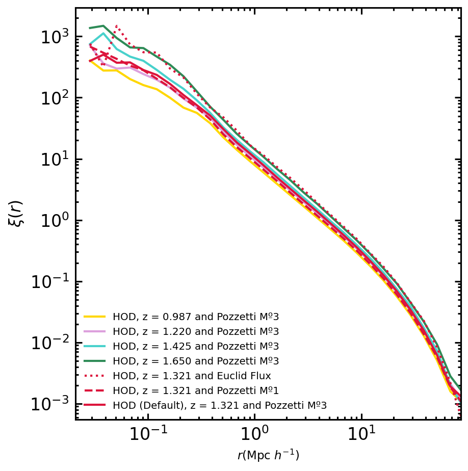
Figure 4: The two point correlation in real space for galaxies generated with HOD models assuming different number densities and redshifts, with different line-styles as indicated in the legend. The three samples at $z=1.3$ with number densities indicated in Table 1 are shown as red lines. The samples with number density fixed to that of Pozzetti model number 3 are shown at different redshifts with varying colours, as indicated in the legend.

In Figure 4 we compare the clustering of galaxies at $z=1.3$ generated with HOD models assuming the three number densities summarised in Table 1 (in three different line-styles). As expected, the clustering at large scales, grows in amplitude with decreasing number density. At $r=10{\rm Mpc}h^{-1}$ there is an increases by a factor of $1.55$ from the sample with the lowest density to the highest.

At small scales, there is a boost in the clustering for the sample with the lowest number density considered. This is partly due to the slight decrease with increasing redshift of the numbers of model satellite H_α-emitters without a central counterpart. Bearing in mind that for this exercise we only used one realisation of the HOD (compared to the $100$ seeds used in the default analysis), we expect that part of these different could also be due to statistical fluctuations.

4.3.2 Evolution with redshift

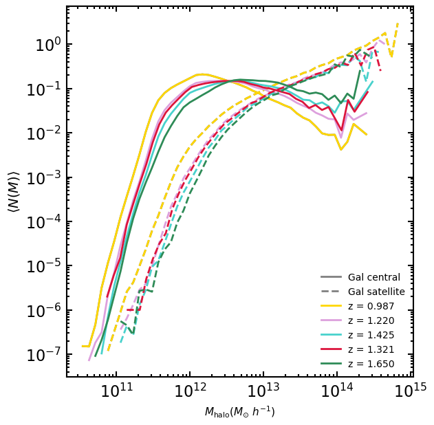
Figure 5: Mean halo occupation distribution for galaxies generated with HOD models at different redshift, as indicated in the legend. The number densities of this samples correspond to those from the diferential luminosity function number 3 from Pozzetti et al. and are summarised in Table 2. The contribution from central galaxies is shown as solid lines and that from satellite galaxies as dashed ones.

dPozzetti nº3	Number density	Flux cutoff
Redshift	$\rm Mpc^{-3}h^{3}$	$\rm erg\,\rm s^{-1}\rm cm^{-2}$
$0.987$	$1.381\times 10^{-3}$	$1.88\times 10^{-16}$
$1.220$	$7.731\times 10^{-4}$	$1.50\times 10^{-16}$
$1.425$	$5.185\times 10^{-4}$	$1.22\times 10^{-16}$
$1.650$	$3.371\times 10^{-4}$	$1.00\times 10^{-16}$

Table 2: The columns in this table contain from left to right: the redshift of each sample; the number densities ($n$) derived from the diferential luminosity function number 3 from Pozzetti et al. at the given redshifts (dPozzetti nº3); and the H_α flux cut used in the SAGE to recover each $n$. Note that for the case of $z=1.3$ we consider a range in redshift, instead of the single redshifts considered here (Table 1).

In this section we discuss how the clustering changes across the Euclid redshift range, $0.9<z<1.8$. For this, we follow the approach by Knebe et al. (2022), where we considered 4 different snapshots in this range ($z=0.99$, $1.22$, $1.42$ and $1.65$) with a number density matched to the differential luminosity function number 3 from Pozzetti et al. (2016). The number density and flux cuts resulting at these four redshifts are listed in Table 2. Note that this procedure is somewhat different to our default $z=1.3$ analysis where we are targeting the average number density over the Euclid redshift range, according to Pozzetti et al. model number 3 (Table 1).

Table 2 shows that the target number densities increase by a factor of $4$ from the lowest at $z=1.65$ to the highest at $z=0.99$. The number density for the sample at $z=1.321$ (Table 1), agrees with this trend, despite being calculated differently. The variation in number density is smaller than the factor of $7$ found between those samples at $z=1.3$ summarised in Table 1. Accordingly, Figure 5 shows smaller variations of the mean HOD than those seen in Figure 1 at fixed redshift.

The typical mass of haloes hosting Euclid-like H_α emitters increases slightly with redshift. Although Figure 5 shows a bigger difference between the sample at $z=0.987$ and the rest, the change in mean HOD with redshift is small. Again, we can expect that part of the differences could be due to statistical fluctuations as we are only using one HOD realisation, instead of the $100$ seed used for our main analysis. This small variation with redshift is consistent with the findings from Rocher et al. (2023a), who showed that DESI OII ELGs do not exhibit significant evolution in the HOD parameters.

Figure 4 also shows a slight increase with redshifts of the clustering at large scales. At $r=10{\rm Mpc}h^{-1}$ there the clustering increases by a factor of $1.62$ from the sample at $z=0.987$ to $z=1.650$.

At small scales we do see in Figure 4 a larger variation in clustering. This might be a consequence of the different slopes of the mean HOD for central galaxies at larger masses. From Figure 5, it is clear how similar the mean HOD for satellite galaxies are.

The results shown in this section are derived with a single seed for each HOD. The level of noise we find for the clustering at small scales, appears to be consistent among the different redshifts.

5 Modelling conformity

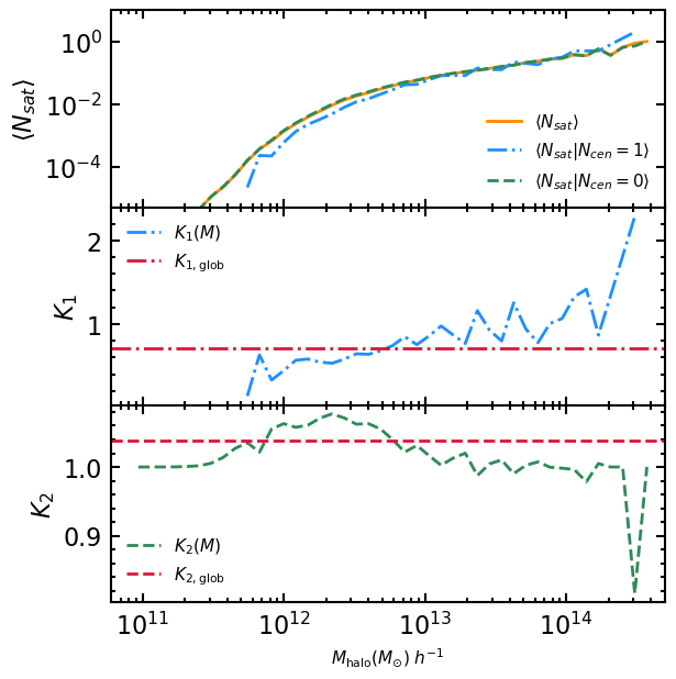
Figure 6: Top: Mean number of satellite galaxies per halo as a function of halo mass: total (orange), with a companion central galaxy of the same type (blue), and without these centrals (green). Middle: The conformity parameter $K_{1}(M)$ per mass bin (Equation 4) and the global conformity factor $K_{1,\rm glob}$ (Equation 6), measured for SAGE_sh Euclid-like H_α emitters, as a function of halo mass. These parameters represent the ratio between the mean number of total satellite galaxies with a central galaxy (shown in blue in the top panel) with respect to the corresponding number of haloes (see Equation 2). Bottom: Similar to the middle panel, but for $K_{2}(M)$ (Equation 5) and the global factor, $K_{2,\rm glob}$

(Equation 7). In this case, these parameters represent the ratio between the mean number of total satellite galaxies without a central galaxy (shown in green in the top panel) with the number of haloes (see Equation 3).

Usually, HOD models assume satellite and central galaxies of a given type to be independent events, i.e., the mean occupation of satellite galaxies does not depend whether or not the central is of the same type. Here we define the 1-halo conformity as deviations from independency, i.e., the mean occupation of satellite H_α emitters depend on having or not a central H_α emitter in that halo.

The phenomenon of galactic conformity refers to the correlation between the properties of neighbouring galaxies (Weinmann et al., 2006). This is thought to happen due to galaxies having a common evolution as baryonic matter collapses within dark matter haloes to form galaxies. Observed galaxies exhibit variations in mass, shape, star formation activity, colors, and ages, and these properties tend to be correlated. It is important to differentiate between one-halo conformity, which measures conformity at small separations within a single halo, and two-halo conformity, which measures conformity at larger separations between central galaxies and neighboring galaxies in adjacent haloes.

Conformity has been detected in simulations (e.g Lacerna et al., 2018; Ayromlou et al., 2023) and there seems to be growing evidence of it from observations (e.g. Rocher et al., 2023a; Gao et al., 2023). Galactic conformity continues to be an active area of study and remains a significant puzzle in our understanding of galaxy formation and evolution.

We define the mean value of satellite galaxies with, $\langle N_{\rm sat}|N_{\rm cen}=1\rangle$, and without a central galaxy, $\langle N_{\rm sat}|N_{\rm cen}=0\rangle$, as:

$$\langle N_{\rm sat}|N_{\rm cen}=1\rangle=\frac{N_{\rm sat,wc}}{N_{\rm h,wc}}=K_{1}\hskip 2.84526pt\langle N_{\rm sat}\rangle$$ (2)

$$\langle N_{\rm sat}|N_{\rm cen}=0\rangle=\frac{N_{\rm sat,w/oc}}{N_{\rm h,w/oc}}=K_{2}\hskip 2.84526pt\langle N_{\rm sat}\rangle\,,$$ (3)

where $N_{\rm sat,wc}$ and $N_{\rm sat,w/oc}$ denote the number of satellites with or without a central H_α galaxy. Note that the total number of satellite galaxies, $N_{\rm sat}$, is the sum of these two values, $N_{\rm sat}=N_{\rm sat,wc}+N_{\rm sat,w/oc}$. The total number of dark matter haloes with and without a central H_α galaxy are $N_{\rm h,wc}$ and $N_{\rm h,w/oc}$, respectively. $\langle N_{\rm sat}\rangle$ is the average value of satellite galaxies in all types of haloes (with and without central galaxies of the given type). $K_{1}$ and $K_{2}$ are the conformity factors.

When there is no conformity, $K_{1}=K_{2}=1$, so the mean number of satellite galaxies is independent of having a central galaxy of the same type, $\langle N_{\rm sat}|N_{\rm cen}=0,1\rangle=\langle N_{\rm sat}\rangle$.

When there is conformity, $K_{1}\neq 1\neq K_{2}$. To model the 1-halo conformity, the average number of satellites should depend on the presence or absence of a central galaxy of the same type.

To investigate conformity, we initially examine whether the average number of satellite galaxies, with or without a central galaxy, constitutes two completely independent events. To achieve this, we calculate the mean values $\langle N_{\rm sat}|N_{\rm cen}=1\rangle$ and $\langle N_{\rm sat}|N_{\rm cen}=0\rangle$ for our SAGE galaxy sample and compare them to the mean value of $\langle N_{\rm sat}\rangle$. In the top panel of Figure 6, we demonstrate that the total number of satellites with and without a central galaxy in our SAGE sample is not reproduced when assuming independence. As a result, we can infer that introducing the concept of conformity is necessary to accurately reproduce these differences. Furthermore, it enables us to demonstrate the crucial role of conformity in replicating the distribution of satellites in SAGE, thus marking it as one of the primary novel findings of our article. It is worth noting that in other studies, such as Lacerna et al. (2018) and Rocher et al. (2023b), they have also found the need to include the conformity property.

5.1 Mass dependent conformity

For a given bin of halo masses, $M_{i}$ and using the above expressions, it is possible to define $K_{1}(M_{i})$ and $K_{2}(M_{i})$ as a function of quantities that we can measure from the reference galaxy catalogue:

$$K_{1}(M_{i})=\frac{N_{\rm sat,wc}(M_{i})}{N_{\rm cen}(M_{i})\ \hskip 2.84526pt\langle N_{\rm sat}(M_{i})\rangle}\,,$$ (4)

$$K_{2}(M_{i})=\frac{1-K_{1}(M_{i})\hskip 2.84526pt\langle N_{\rm cen}(M_{i})\rangle}{1-\langle N_{\rm cen}(M_{i})\rangle}\,.$$ (5)

The above conformity factors, $K_{1}(M_{i})$ and $K_{2}(M_{i})$, can be computed using these equations by inserting the galaxy/halo counts measured in our simulation. These factors are then used in a HOD prescription for each mass bin. In practice, what we need is to first sample the Bernoulli PDF for centrals in order to determine whether we have $N_{\rm cen}=0$ or $N_{\rm cen}=1$ in a given halo (see PDF description in subsubsection 4.1.3) and then modify $\langle N_{\rm sat}\rangle$ according to Equation 3 or Equation 2, respectively. Subsequently, we would sample the Poisson distribution (again subsubsection 4.1.3) from the modified $\langle N_{\rm sat}\rangle$ ($=\langle N_{\rm sat}\lvert N_{\rm cen}\rangle$) and continue with the rest of steps of the HOD (subsection 4.1).

In the middle panel of Figure 6, we can observe the conformity parameter $K_{1}(M)$ (Equation 4) for our SAGE_sh H_α emitters sample as a function of halo mass. These parameters represent the relationship between the average number of total satellite galaxies associated with a central galaxy and the overall average number of satellites, depicted in blue for $K_{1}(M)$. This comparison indicates the presence of conformity, i.e., how much it deviates from the scenario where the existence of a satellite galaxy and a central galaxy are two independent events (that would be represented by $K_{1}(M)=1$). Then, in the bottom panel, similar analyses are performed, but this time for $K_{2}(M)$ (Equation 5). In this case, these parameters represent the ratio between the mean number of total satellite galaxies without a central galaxy and the overall average number of satellites, shown in green for $K_{2}(M)$.

5.2 Global conformity

As an alternative, we consider global conformity factors, $K_{1,\rm glob}$ and $K_{2,\rm glob}$, that are assumed constant for a given reference galaxy catalogue and to be the same for all halo masses. $K_{1,\rm glob}$ and $K_{2,\rm glob}$ are then constants in Equation 2 and Equation 3. In this case, the global conformity factors are computed as:

$$K_{1,\rm glob}=\frac{\sum_{i=1}^{n}{N_{\rm sat,wc}(M_{i})}}{\sum_{i=1}^{n}\langle N_{\rm cen}(M_{i})\rangle\hskip 2.84526ptN_{\rm sat}(M_{i})}\,,$$ (6)

$$K_{2,\rm glob}=\frac{\sum_{i=1}^{n}{N_{\rm sat,w/oc}(M_{i})}}{\sum_{i=1}^{n}(1-\langle N_{\rm cen}(M_{i})\rangle)\hskip 2.84526ptN_{\rm sat}(M_{i})}\,,$$ (7)

where $i$ indicates each of the different mass bins considered. The somewhat complicated expressions above are a consequence of populating the mean HOD $\langle N_{\rm sat}\rangle$ in bins of halo mass, hence, with Equation 3 and Equation 2 also applied in mass bins. This implies that we can not compute the global factors, $K_{1,\rm glob}$ and $K_{2,\rm glob}$, by simply dropping the mass dependence from Equation 4 and Equation 5. Instead, we need to compute them in individual bins and then do the sum indicated in Equation 6 and Equation 7.

The middle panel of Figure 6 shows the global conformity factor $K_{1,\rm glob}$ (Equation 6) for our SAGE_sh H_α emitters sample. And the bottom panel the other global factor, $K_{2,\rm glob}$ (Equation 7). The global conformity factors, $K_{1,\rm glob}$ and $K_{2,\rm glob}$, roughly correspond to the respective mean values of the mass-dependent conformity ones, $K_{1}(M)$ and $K_{2}(M)$.

Sample	Redshift	$K_{1,\rm glob}$	$K_{2,\rm glob}$
Pozzetti nº1	$1.3$	$0.799$	$1.034$
Pozzetti nº3	$\mathbf{1.3}$	$\mathbf{0.708}$	$\mathbf{1.038}$
Euclid flux	$1.3$	$0.618$	$1.033$
dPozzetti nº3	$0.987$	$0.741$	$1.033$
dPozzetti nº3	$1.220$	$0.717$	$1.035$
dPozzetti nº3	$1.425$	$0.701$	$1.040$
dPozzetti nº3	$1.650$	$0.718$	$1.042$

Table 3: Global conformity parameters, $K_{1,\rm glob}$ (Equation 6) and $K_{2,\rm glob}$ (Equation 7) for galaxies produced with HOD models at different redshifts and with number densities obtained either in a range of redshifts, first three rows (Table 1) or from a differential luminosity function (Table 2). Our default choice is the sample at $z=1.3$ with number density matching that of Pozzetti model number 3 in a range of redshifts. This is indicated by using bold face in the table.

We find $K_{1,\rm glob}=0.708$ and $K_{2,\rm glob}=1.038$, implying that we detect conformity of the order of $\sim 15-20$%. These values are summarised in Table 3, together with those derived for galaxy samples with the other two number densities considered in this study (see Table 1).

The global conformity factors remain remarkably constant for samples of H_α emitters with different number densities. The variations are below $20$% for $K_{1,\rm glob}$ and below $1$% for $K_{2,\rm glob}$. This suggests that the mechanisms that drives conformity might depend weakly on environment. This is in line with the proposal of spectral emission lines coming from star forming regions being triggered by merging events (Yuan et al., 2023b).

The conformity global factors, $K_{1,\rm glob}$ and $K_{2,\rm glob}$, obtained for samples at different redshifts are summarised in Table 3. We find variations below $5\%$ for $K_{1,\rm glob}$ and below $1\%$ for $K_{2,\rm glob}$. The results suggest that there is no evolution in conformity in the explored redshift range, $0.987<z<1.650$.

5.3 Clustering

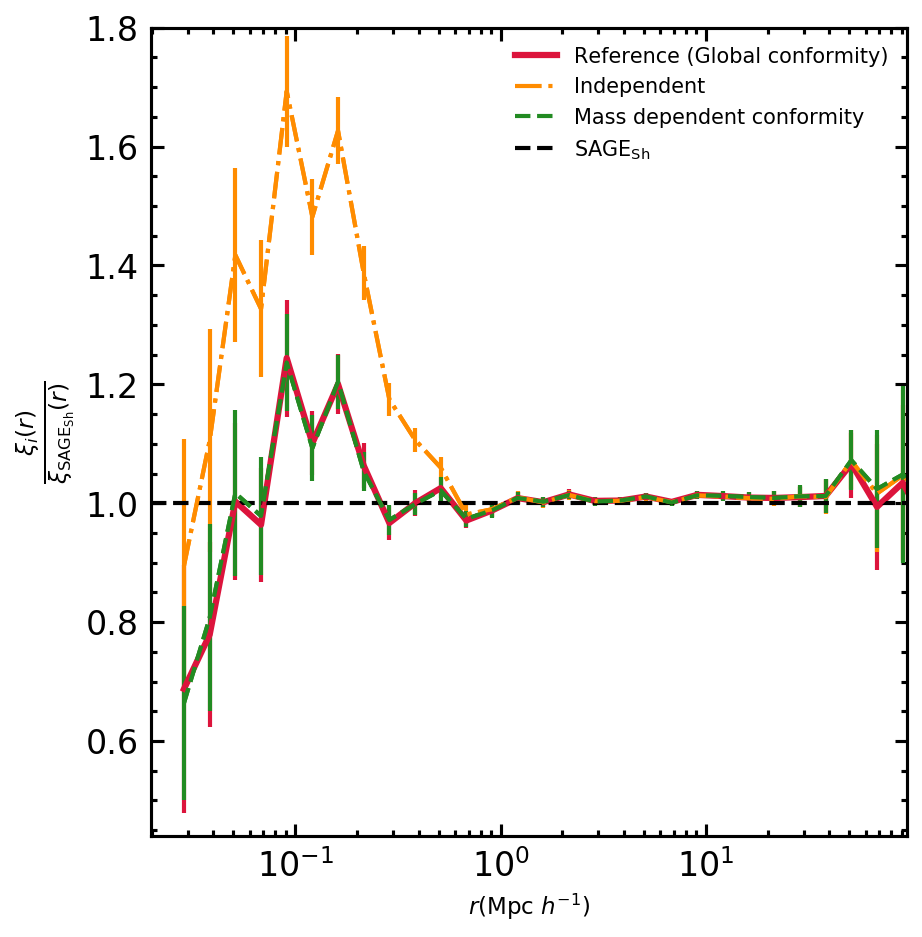
Figure 7: Ratios of the real space two-point correlation functions from galaxy catalogues generated with different HOD models with respect to that from the SAGE_sh reference galaxy. The result from the proposed HOD model (§ 4.3), which uses global conformity factors, is shown in red. Two modifications of this model are also shown: one with no conformity (centrals and satellites are treated as independent events), shown in orange; and one using mass dependent conformity factors, shown in green. Note that the three HOD catalogues use an analytical function to model the radial distribution of satellite galaxies (§ 14). The error bars are calculated as the standard deviation of 100 realisations.

After computing the values of $K_{1}$ and $K_{2}$, either as a global factor or as a function of mass, we apply Equations 2 $\&$ 3 to our HOD model, based on either the global conformity or the mass-dependent conformity, respectively.

Subsequently, we assess their clustering and compare, in Figure 7, the results to a scenario without conformity (orange dotted dashed). The dot-dashed green line illustrates the scenario where $K_{1}$ and $K_{2}$ are dependent on the mass of the bins, while the solid red line corresponds to the global factor conformity. First of all, it is noticeable that in the case of independence, the largest deviation from the reference sample in terms of clustering occurs around $r\sim 0.1,\text{Mpc},h^{-1}$, resulting in an approximately $\sim 60\%$ difference. However, by incorporating conformity, we mitigate this difference by $\sim 40\%$ at this scale. Moreover, we observe that both implementations of conformity yield similar outcomes, significantly superior to the scenario without considering conformity. The clustering is found nearly indistinguishable between the two models proposed for conformity. Consequently, for the sake of simplicity, we opt for using global conformity factors as our default modeling approach. It is important to emphasize that the results regarding the necessity of including the conformity property align with what has been found in other studies, as mentioned in Lacerna et al. (2018) or Rocher et al. (2023b). In the latter, a mean satellite occupation function was obtained that aligns with physically motivated models of OII galaxies (ELG) only if conformity between centrals and satellites is introduced. This implies that the occupation of satellites is conditioned by the presence of central galaxies of the same type. It turns out that this aligns with what we obtain in this article, while using very different angles.

6 The radial profile of satellite galaxies

The distribution of substructure in dark matter haloes has been accurately described by either a Navarro-Frenk-White profile (NFW, Navarro et al., 1997) or an Einasto profile (Einasto, 1969). However, the distribution of galaxies within haloes could be biased with respect to that of dark matter (e.g Yuan et al., 2023a; Rocher et al., 2023a; Hadzhiyska et al., 2023).

Central galaxies are placed in the center of potential of the dark matter halo, so we focus here on satellite galaxies and how they are distributed with respect to their center of halo.

In this work, we first study the spatial distribution of Euclid-like H_α satellite galaxies within dark matter haloes in SAGE_sh. Then we explore how to best use the measured distribution to inform HOD models with the aim to reproduce the SAGE_sh 1-halo term clustering.

The radial profile of SAGE_sh satellite H_α emitters is shown in Figure 8 as filled circles. This plot shows the number of satellite galaxies as a function of their distance to the central galaxy, $r=|\vec{r}|=|\vec{r}_{\rm sat}-\vec{r}_{\rm h}|$. Note that we have verified the existence of a displacement between the position of the central galaxy and the center of the halo. However, we have studied these differences, and they are smaller than $1\times 10^{-5}$ for all central galaxies, so we can assume that $\vec{r}_{\rm cen}=\vec{r}_{\rm h}$. Satellite galaxies in SAGE_sh are preferentially placed at a distance of $\sim 0.2{\rm Mpc}h^{-1}$ from their central galaxy.

In Figure 8, we present the radial profile as a function of the relative distance to the halo, $r$, because we have found that this approach provides an HOD model clustering closer to the reference SAGE_sh sample. This result is shown in 9. It is clear from this figure that the 1-halo clustering is better recovered when the radial profile as a function of $r$ is best matched, instead of $r/R_{\rm s}$ or $r/R_{\rm vir}$. This is a surprising result as haloes of different sizes and masses are being mixed in the radial profile shown in Figure 8, as a function of $r$.

Typically, HOD models place satellite galaxies in dark matter haloes assuming the NFW profile given the concentration (or mass) of the halo (e.g. Zheng et al., 2005). This is typically done halo-by-halo. An other commonly used option is to use the positions of dark matter particles (e.g. Avila et al., 2020; Rocher et al., 2023a).

Our aim is to have an HOD model with galaxies clustered as close as possible to that from SAGE_sh, in small scales. To achieve this, we explore HOD models with different ways of placing satellite galaxies within haloes: (i) NFW profiles using the concentration from each halo (§ 6.1, NFW halo-by-halo); (ii) NFW and Einasto curves fitted to the $r/R_{\rm s}$-stacked profiles (§ 6.2); (iii) NFW and Einasto curves fitted to the $r/R_{\rm vir}$-stacked profile (§ 6.3); (iv) radial profile from SAGE_sh, as a function of $r$, using it either directly as a discrete distribution function or to fit an analytical function (§ 6.5).

Figure 8 presents the radial distribution of galaxies modelled with all the approaches described above, together with the SAGE_sh distribution. From this figure, it is clear that the first three approaches cannot reproduce the radial profile of satellite galaxies in SAGE_sh. A similar conclusion was reached by Qin et al. (2023) also using the SAGE SAM to study the distribution of galaxies. In their work they applied their proposed extended profile to SSDS DR10 group catalogue galaxies.

The different HOD approaches described above are implemented following a similar method. For each halo, we generate a number of random values equal to the number of satellite galaxies assigned to that halo, which we then transform to a distance $x$ using an inverse cumulative distribution sampling of the profile (in terms of $N(x)\propto x^{2}\rho(x)$). This distance $x$ can be $r/R_{\rm vir}$, $r/R_{\rm s}$ or $r$ depending on the chosen independent variable in each prescription. The first two distances can be transformed into $r$, given the halo $R_{\rm vir}$ or $R_{s}$. Once we have $r$, we place the satellite galaxies by randomly sampling the angular position with respect to the halo center.

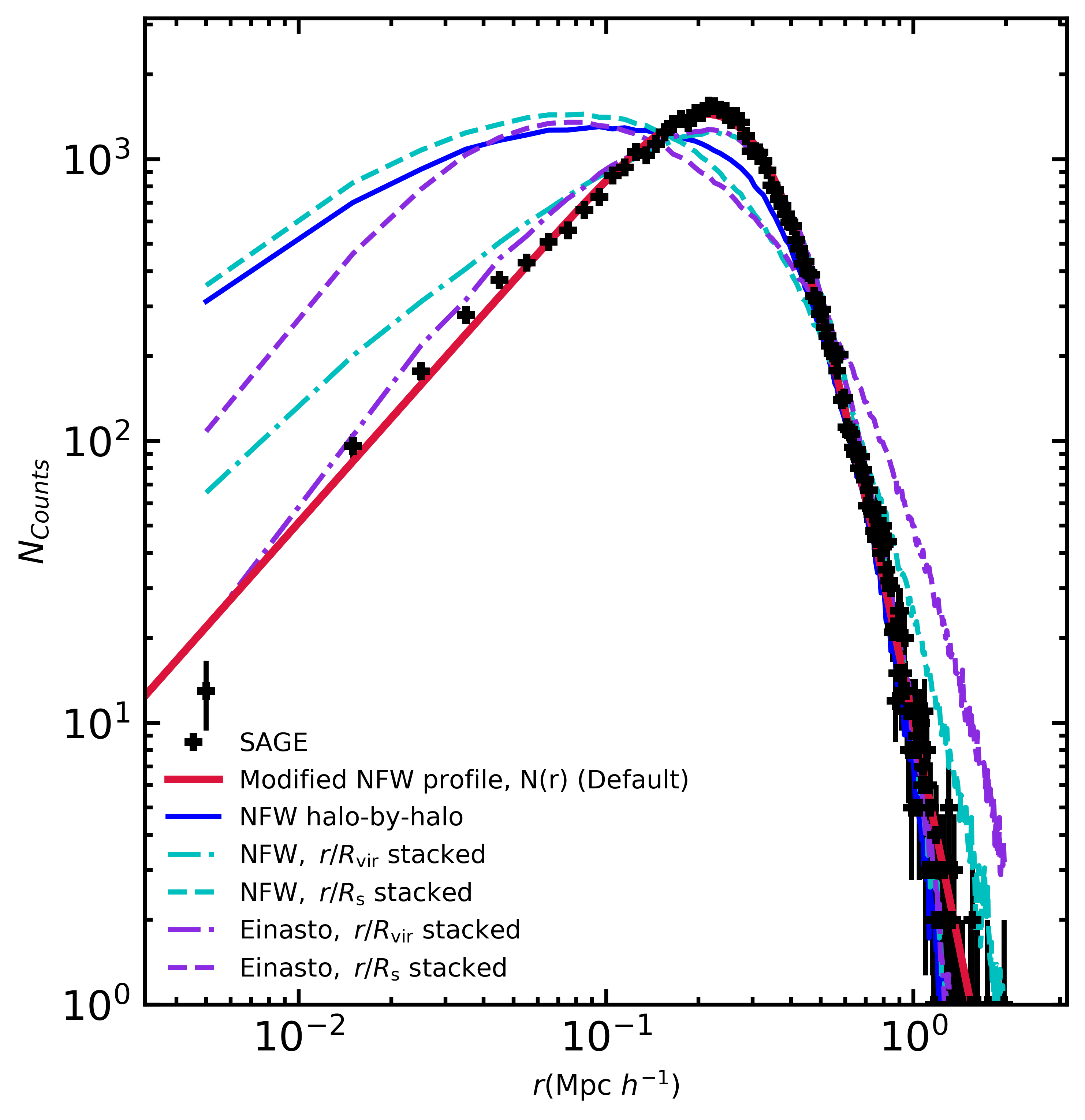
Figure 8: Radial profile for satellite galaxies as a function of their distance, $r$, to the center of their host halo. Euclid-like H_α emitters from SAGE_sh are shown as filled symbols with Poisson error bars. The lines correspond to catalogues produced with different HOD models, as indicated in the legend. The results from our proposed HOD model (§ 4.3), which uses an analytical function (Equation 14) to fit the radial distribution of SAGE_sh satellite galaxies, is shown in red. Five modifications of this model are also shown in the plot: a model assuming a NFW distribution given the concentration of each halo (solid blue line); models assuming a NFW density profile fitted to reprocude the average SAGE_sh one as a function of $r/R_{\rm vir}$ (dash-dotted blue line) and $r/R_{\rm s}$ (dashed blue line); models assuming an Einasto profile fitted to reproduce the average SAGE_sh one as a function of $r/R_{\rm vir}$ (dash-dotted purple line) and $r/R_{\rm s}$ (dashed purple line). Note that the binning is linear but we have plot in logarithmic scale to properly appreciate the change of slopes.

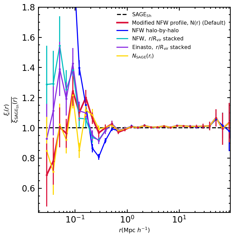
Figure 9: Ratios of the real space two-point correlation functions from galaxy catalogues generated with different HOD models with respect to that from the SAGE_sh reference galaxy sample. The results from our proposed HOD model (§ 4.3), which uses an analytical function (Equation 14) to fit the radial distribution of SAGE_sh satellite galaxies, is shown in red. Four modifications of this model are also shown in the plot, with similar colours to those shown in Figure 8. Error bars are calculated as the standard deviation of 100 realisations with changing seeds for the generators of random numbers.

6.1 NFW halo-by-halo: Sampling individual halo profiles

HOD models usually place satellite galaxies within haloes following the distribution of dark matter itself (e.g. Avila et al., 2018). This is often described by a Navarro–Frenk–White (NFW) profile, which was derived from dark matter only N-body simulations (Navarro et al., 1997). The NFW profile describes the density of dark matter, $\rho_{\rm NFW}$, as a function of distance to the center of a halo, $r$:

$$\rho_{\rm NFW}(r)=\frac{4\,\rho_{\rm s}}{\frac{r}{R_{\rm s}}\left(1+\frac{r}{R_{\rm s}}\right)^{2}}\ ,$$ (8)

where $R_{\rm s}$ is the scale radius provided by Rockstar, and $\rho_{\rm s}$ is the mass density at this radius. The halo concentration, $C$, relates the virial and scale radii of haloes, $R_{\rm vir}=CR_{\rm s}$.

Given a halo concentration, the NFW can be sampled in a halo-by-halo basis. We have followed this method to construct catalogues of Euclid-like H_α emitters. In Figure 8 we compare the global radial profile for satellite galaxies from this catalogue (dark blue solid line, NFW halo-by-halo) with that from SAGE_sh. The differences are large, in particular below $0.1h^{-1}{\rm Mpc}$. At these scales, we obtain differences over $70\%$ compared to our SAGE_sh sample. The difference increases for smaller values of $r$.

The NFW halo-by-halo clearly fails to reproduce the global radial profile of SAGE_sh satellite galaxies. This difference results in a very strong clustering at scales below $\sim 0.2h^{-1}{\rm Mpc}$. The NFW halo-by-halo results in galaxy clustering over a factor of $2$ above the clustering measured for SAGE_sh galaxies at scales below $0.1h^{-1}{\rm Mpc}$ (Figure 9). This is of great importance, as the NFW halo-by-halo approach is very commonly used one in the literature to populate halo catalogues from large simulations.

6.2 $r/R_{\rm s}$-stacked profiles

We have fitted the SAGE_sh $r/R_{\rm s}$-stacked satellite profile with single NFW(Navarro et al., 1997) and Einasto (Einasto, 1969) parametrisations. To construct the stacked profile from the SAGE_sh sample we start by converting the counts of satellite galaxies as a function of distance to the central galaxy, $N(r)$, into densities, with $\rho=N(r)/(4\pi r^{2}{\rm d}r)$. We use a binning of ${\rm d}r=0.1$.

In the previous section, we introduced the NFW parametrisation of radial profiles (Equation 8). The Einasto parametrisation can be written as a function of the scale radius, $R_{\rm s}$, as follows:

$$\rho_{\rm Ein}(r)=\rho_{\rm s}\hskip 2.84526pte^{-\frac{2}{\alpha}[(\frac{r}{R_{\rm s}})^{\alpha}-1]}\,,$$ (9)

where $\rho_{\rm s}$ is the mass density at $r=R_{\rm s}$ and $\alpha$ determines the curvature of the profile.

When fitting the SAGE_sh $r/R_{\rm s}$-stacked profiles we aim to recover the total number of satellite galaxies. To achieve this, the NFW (Equation 8) and Einasto (Equation 9) parametrisations must be integrated up to $r=R_{\rm vir}$, which is considered the edge of the halo. Thus, we ensure the total number of satellite galaxies, $N_{\rm sat}$, is preserved by imposing:

$$N_{\rm sat}=R_{\rm s}^{3}\int_{0}^{\left(\frac{r}{R_{\rm s}}\right)=\frac{R_{\rm vir}}{R_{\rm s}}\equiv C}4\pi\left(\frac{r}{R_{\rm s}}\right)^{2}\rho\left(\frac{r}{R_{\rm s}}\right){\rm d}\left(\frac{r}{R_{\rm s}}\right)\,.$$ (10)

When fitting the NFW and Einasto parametrisations, we find the halo concentration, $C=R_{\rm vir}/R_{\rm s}$, that gives the closest value of $N_{\rm sat}$ to the SAGE_sh one. Note that the concentration appears as an integration limit in Equation 10. For both parametrisations, $\rho_{0}$ provides the normalisation of the fit to the SAGE_sh $r/R_{\rm s}$-stacked satellite profile. The NFW profile has the halo concentration as the only free parameter, while the Einasto one also has $\alpha$ as a second free parameter.

For performing the fit to the NFW profile, we allow the halo concentration to vary from $0.1$ to $10$. This truncation is chosen based on the scarcity of satellite galaxies, $N\lesssim 1$, beyond this limit. This choice is conservative, compared with the results from Ramakrishnan et al. (2019) where they used dark matter simulations to measure the distribution of different halo properties. In their study, the halo concentration is found between $0$ and $\sim 30$.

To determine the parameters that yield the best fit to the SAGE_sh $r/R_{\rm s}$-stacked profiles, we iterate through different values of halo concentration, $C_{i}$, which gives the upper limit of the integration in Equation 10. The parameters yielding the lowest $\chi^{2}$ per data point (see below) value are selected as the optimal fit. The $\chi^{2}$ value is determined using the following expression:

$$\chi^{2}=\sum\frac{(\rho_{\rm SAGE_{sh}}-\rho)^{2}}{\sigma^{2}}\,,$$ (11)

where we assume a Poisson error on the counts, which translates to an uncertainty on the density profile of

$$\sigma=\frac{\sqrt{N}}{4\pi\left(\frac{r}{R_{\rm s}}\right)^{2}\Delta\left(\frac{r}{R_{\rm s}}\right)}\ .$$ (12)

We perform the integration within $\Delta(r/R_{\rm s})=0.05$ bins. Thus, for smaller $C_{i}$ values, the number of data points used to evaluate the functions will be fewer compared to larger ones, due to the profile cutoff set by this integration limit (see Equation 10). To address this differences, we normalize the $\chi^{2}$ value dividing it by the total number of bins within each interval. We minimize this normalised quantity.

In the case of an Einasto profile, a combination of $C_{i}$ and $\alpha_{i}$ values are sampled from a grid. For $C_{i}$, we follow the same approaches as for NFW, and consider $\alpha_{i}$ values from $0.1$ to $2$, incremented by $\Delta\alpha=0.01$

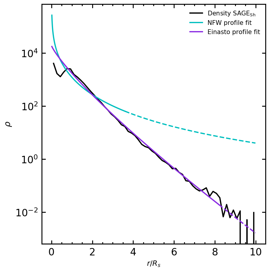
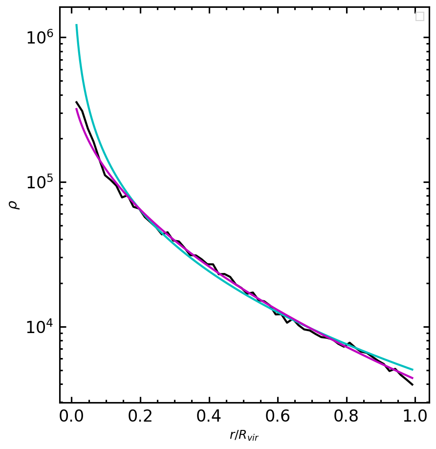
Figure 10: Density profiles of the SAGE_sh Euclid-like H_α emitters as a function of $r/R_{\rm s}$, left, and $r/R_{\rm vir}$, right, in black, together with fits using either NFW, in blue, or Einasto profiles, in purple. In the case of density profiles as a function of $r/R_{\rm s}$, the average concentration, $\langle C\rangle$, is a free parameter that appears as an integration limit (see Equation 13). We show as solid lines the fit up to $\langle C\rangle$, beyond this value we show dashed lines. Note that in this case we are effectively averaging different parts of haloes with different sizes.

Table 4 presents the best fit parameters to the SAGE_sh $r/R_{\rm s}$-stacked satellite profile for both NFW and Einasto profiles. The left panel of Figure 10 show the best fit profiles compared to the Euclid-like H_α emitters. We can observe that the Einasto density profile fits reasonably well, whereas the NFW profile is far from being a good fit.

$r/R_{\rm s}$	NFW	Einasto
$\rho_{0}\left(\frac{h^{3}}{\rm Mpc^{3}}\right)$	1227	1742
C	3.60	8.20
$\alpha$	-	0.83
$r/R_{\rm vir}$
$\rho_{0}\left(\frac{h^{3}}{\rm Mpc^{3}}\right)$	3941	10593
C	0.89	1.49
$\alpha$	-	0.51

Table 4: Best fit parameters to the SAGE_sh $r/R_{\rm s}$ and $r/R_{\rm vir}$-stacked satellite profile for both NFW and Einasto profiles. It should be noted that the best fit of NFW for C is very similar to what we obtain by averaging the $C_{i}$ values of haloes containing satellite galaxies.

Finally, we generate the corresponding mocks using these fitted $r/R_{S}$ profiles. In Figure 8, we can observe the profiles in terms of $r$ (dashed violet and cyan). We find that even when utilizing our fitted $r/R_{\rm s}$-stacked profiles, we still achieve a poor $N(r)$ curve, akin to the one obtained through the halo-by-halo sampling approach (blue curve). This is particularly striking for the Einasto profile, which showed a good fit in the stacked $\rho(r/R_{s})$ profile.

6.3 $r/R_{\rm vir}$-stacked profiles

In order to address the next scenario, we begin by rewriting equations 8 and 9 in terms of the virial radius of the haloes with $R_{\rm vir}=C\hskip 2.84526ptR_{\rm s}$. The viral radius is defined as the radius that contains a mass with a virial overdensity, defined by $\rho$ from Bryan & Norman (1998) and internally computed by Rockstar. It is considered the size of the halo, hence objects beyond this radius are considered outside the halo. By now stacking the profile in terms of $r/R_{\rm vir}$ we are encapsulating the information of the size of each halo (instead of the concentration as in subsection 6.2).

Following a similar procedure to the previous case, we observe that both classical models have the same number of free parameters and normalization parameters for fitting using r/$R_{\rm vir}$. However, in this situation, the free parameter C does not appear as an integration limit, but rather as a component within the density profile functions for both models. To ensure the conservation of the total number of satellites, we integrate these theoretical expressions up to r = $R_{\rm vir}$, leading to the following equivalences:

$$N_{\rm sat}=R_{\rm vir}^{3}\int_{0}^{\left(\frac{r}{R_{\rm vir}}\right)=\frac{R_{\rm vir}}{R_{\rm vir}}=1}4\pi\left(\frac{r}{R_{\rm vir}}\right)^{2}\rho\left(\frac{r}{R_{\rm vir}}\right){\rm d}\left(\frac{r}{R_{\rm vir}}\right)\$$ (13)

It is important to note that, in this case, when performing the fit, we truncate the density profile obtained from our sample of satellite galaxies up to $r=R_{\rm vir}$, as there are very few satellite galaxies beyond this value. Technically, there should not be any. By definition, there are no subhaloes outside the virial radius, but there are some exceptions, likely due to how the merger trees are constructed with ConsistentTrees (Behroozi et al., 2013b).

For the fitting, we use the same procedure as in the previous section, with a few differences. Now, C does not appear as an integration limit but is explicit present in the functions of both models. Likewise, in this case we always evaluate the number of data points from our histograms ($0\leq r\leq R_{\rm vir}$ with $\Delta(r/R_{\rm vir})$ = 0.01), eliminating the need for normalization by the total number of bins.

In the right panel of Figure 10, we observe the fittings achieved by the parameter set that minimizes the $\chi^{2}$ of the classical models (Einasto and NFW) with respect to our sample of SAGE satellite galaxies, when stacking the profiles on the variable $r/R_{\rm vir}$. The resulting parameters for both models are shown in Table 4. For this case, we can confirm that a decent qualitative fit has been achieved for both the NFW and Einasto profiles, unlike the $r/R_{\rm s}$ case. However, the Einasto profile still provides a better fit, as expected, given that it includes one more free parameter.

It is worth noting that even though both models share the same physical parameters ($\rho_{s}$, $C$, $\alpha$), the values obtained differ when using $r/R_{\rm s}$ or $r/R_{\rm vir}$ as our variable (see Table 4). These differences stem from the lack of a direct correlation between the variables $R_{\rm s}$ and $R_{\rm vir}$, with a Pearson correlation coefficient of only $r_{\rm R_{\rm vir},R_{\rm s}}$ = 0.36. As a result, we find a great dispersion between these variables, between these and the concentration $C$ and also between all those quantities and the $r$ found in the ELGs. This non-univocal relation between the variables considered, makes possible the differences observed in the goodness of fit and best fit parameters when considering a fit to an $r/R_{\rm S}$-stacked profile or an $r/R_{\rm vir}$-stacked profile.

This level of dispersion is consistent with what has been previously presented in Salvador-Solé et al. (2023). In the aforementioned article, various models with distinct simulations and redshift values, showing an existence of a concentration dispersion in relation to the mass of haloes. The resulting $C-M_{200c}$ diagrams can be extrapolated using the dispersion we discovered for the variables $R_{\rm s}$ and $R_{\rm vir}$, which are correlated with mass.

In Figure 8, we can observe the profiles as a function of distance ($r$) that we have obtained from the generated mocks using the average fits of the NFW and Einasto density profiles in terms of $r/R_{\rm vir}$, as described in this subsection. As observed, both Einasto and NFW models show better results when the fits are performed in terms of $r/R_{\rm vir}$ (dotted dashed) compared to when we use $r/R_{\rm s}$ (dashed), in comparison with our reference, SAGE (black dots). It is also possible to appreciate a better adjustment of the Einasto model with respect to the NFW model, at least on the low-$r$ side, in line with the findings in Figure 10. In light of these findings, when studying the clustering of the different samples, we will only show results of the $r/R_{\rm vir}$-fitted classical profiles (and not the $r/R_{\rm S}$ ones), to avoid overcrowding our figure.

The differences observed in the profile as a function of distance $N(r)$ translate to differences in the observed galaxy clustering. These differences are reflected in Figure 9, where a strong clustering is observed at scales below $\sim 0.1h^{-1}{\rm Mpc}$. This difference reaches almost $\sim 40\%$ for both the NFW and Einasto cases at $r\sim 0.1h^{-1}{\rm Mpc}$. Furthermore, we can confirm that the Einasto fit proves to be superior to the NFW concerning small scales ($<0.1h^{-1}{\rm Mpc}$), consistent with the results obtained earlier in this subsection.

6.4 The inherent SAGE_sh distribution $\rho_{\rm SAGE_{sh}}(r)$ profile.

In order to achieve a better fit on the small scale in terms of clustering compared to the various prescriptions discussed in the previous subsections, we make use of the inherent SAGE_sh distribution $\rho_{{\sc SAGE}}(r)$ profile. This allows us to determine the discrete distribution profile (in a histogram) of our sample of satellite galaxies from SAGE_sh. We use linear binning with a bin size of $\Delta r=0.01h^{-1}$Mpc. We then use this histogram as a discrete distribution function to generate new catalogs of satellite galaxies with their respective positions. In Figure 9, we can see the clustering we obtain for this case (gold curve). Where it can be observed that it corresponds to the best results in terms of fitting the small scale, below $r=1h^{-1}{\rm Mpc}$. It is worth noting that for $r\sim 0.1h^{-1}{\rm Mpc}$, this difference is below $25\%$.

6.5 Extending NFW for an average $\rho(r)$profile.

In this section, we present an analytical expression that describes the SAGE_sh profile with greater accuracy. Since the previous prescriptions did not perform adequately in reproducing the radial profile ($N(r)$) of our SAGE_sh satellite sample, we now attempt to directly fit the profile based on the variable $r$. This variable is the most closely related one to observable quantities and during our study we have found that the profiles in $r$ are a better indicator of the measured clustering. For example, as we see in subsection 6.4, when we use the $N(r)$ measured directly from SAGE_sh, we achieved good results in terms of clustering. Motivated by this, we now perform an analytical fit to $N(r)$ that may make more portable our results to other models and easily implementable in different simulations. After some search, we found that the following analytical function describes well the $N(r)$ profile of SAGE_sh:

$$N(r)=N_{0}\cdot\left(\frac{r}{r_{0}}\right)^{\alpha}\left(1+\left(\frac{r}{r_{0}}\right)^{\beta}\right)^{\kappa}\,,$$ (14)

with $N_{0}=3928.273$ , $r_{0}=0.34h^{-1}{\rm Mpc}$, $\alpha=1.23$, $\beta=3.19$ and $\kappa=-2.1$. Note that these parameters are free, and this case is applicable to our binning in $\Delta r=0.01$, thus the normalization would change with the binning.

In Figure 8 it is evident that our implemented analytical function (solid red line) offers a better fit to describe the SAGE profile compared to all the other used prescriptions.

The derived analytic expression can be interpreted as a generalization of the NFW density profile:

$$\rho(r)=4\rho_{0}\cdot\left(\frac{r}{r_{0}}\right)^{\alpha-2}\left(1+\left(\frac{r}{r_{0}}\right)^{\beta}\right)^{\kappa}\ ,$$ (15)

where $\rho_{0}=N_{0}/16\pi r_{0}^{2}$. When $\alpha=3$, $\beta=1$ and $\kappa=-2$, the expresion above is reduced to the classical NFW profile (8). In this case, the free parameter $r_{0}$ would correspond to the $R_{s}$ variable in the NFW density profile, and our definition of $\rho_{0}$ with the $\rho_{s}$ variable.

Figure 9 shows how reproducing the global radial profile of SAGE_sh satellite galaxies using an analytical extension of the NFW density profile yields similar results to those we obtain if we use the histogram of the distribution profile of satellite galaxies in SAGE_sh (gold curve). For small scales, below $r=1h^{-1}{\rm Mpc}$, our analytical expression (red curve) achieves a clustering that reproduces that of SAGE_sh within $\sim 25\%$.

Sample	Redshift	$\alpha$	$\beta$	$\kappa$	$r_{0}$
Pozzetti nº1	$1.3$	$1.29$	$2.98$	$-2.21$	$0.31$
Pozzetti nº3	$\mathbf{1.3}$	$\mathbf{1.23}$	$\mathbf{3.19}$	$\mathbf{-2.1}$	$\mathbf{0.34}$
Euclid flux	$1.3$	$1.1$	$3.17$	$-2.49$	$0.44$
dPozzetti nº3	$0.987$	$1.35$	$2.53$	$-2.56$	$0.33$
dPozzetti nº3	$1.220$	$1.24$	$3.05$	$-2.16$	$0.34$
dPozzetti nº3	$1.425$	$1.17$	$3.27$	$-2.09$	$0.35$
dPozzetti nº3	$1.650$	$1.16$	$3.05$	$-2.63$	$0.39$

Table 5: Values of the free parameter in Equation 14 and Equation 15 that best fit the radial profiles of our reference samples of Euclid-like H_α emitters for samples at different redshifts and with number densities obtained either in a range of redshifts, first three rows (Table 1) or from a differential luminosity function (Table 2). Our default choice is the sample at $z=1.3$ with number density matching that of Pozzetti model number 3 in a range of redshifts. This is indicated by using bold face in the table.

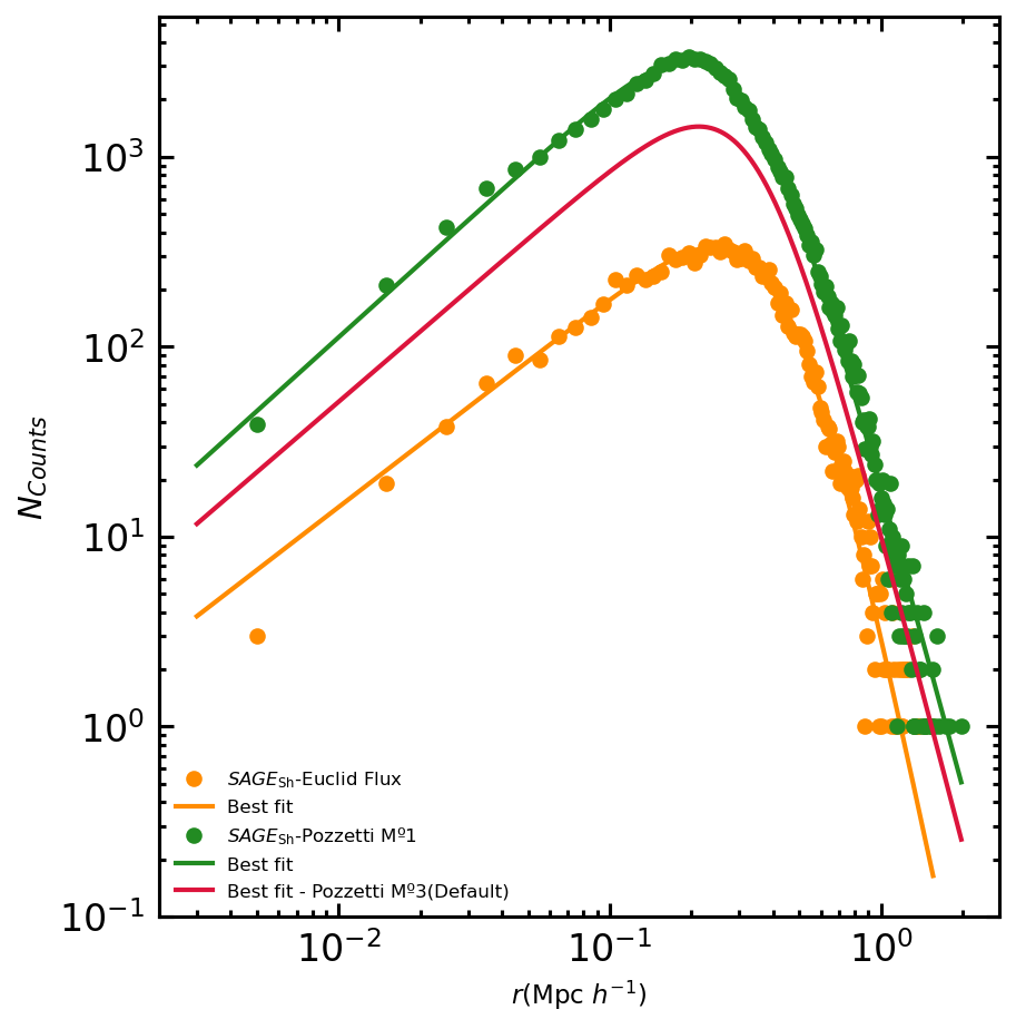
Figure 11: Radial profile for satellites at $z=1.3$ from our reference sample of Euclid-like H_α emitters modelled by SAGE_sh (filled symbols) assuming two number densities: Pozzetti model number 1 and Euclid flux (Table 1), as indicated in the legend. These reference profiles are compared with their best fits to the analytical function for the radial profiles described by Equation 14 (Table 5). For reference, the profile from the default case, Pozzetti model number 3, is shown as a red line.

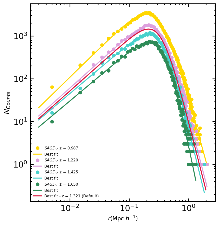
Figure 12: Radial profile for satellites at different redshift from our reference sample of Euclid-like H_α emitters modelled by SAGE_sh (filled symbols) assuming number densities matching the differential luminosity function number 3 from Pozzetti et al. (Table 2). These are compared with the corresponding best fits to the analytical function described in Equation 14 (Table 5). For reference, the profile from the default case, Pozzetti model number 3 in a range of redshifts centered at $z=1.3$, is shown as a red line.

In Figure 11 we compare the radial profile of satellites from the three SAGE_sh H_α samples at $z=1.3$ with different number densities (Table 1). The radial profiles for the three SAGE_sh samples exhibit the same shape with varying normalisation, as expected from the change in number density. At $r=0.21{\rm Mpc}h^{-1}$, the value associated with the maximum number of counts for our reference sample, the count number increases by a factor of $2.19$ from the reference sample to that with the highest density. This factor practically coincides with the ratio of total satellite galaxies between both samples, $2.04$. The count number increases by a factor of $4.15$ from the sample with the lowest density to the reference one; approaching the value corresponding to the ratio of total satellite galaxies for that case, which is $3.73$.

The three samples with varying number density at $z=1.3$ are well described by our proposed extended NFW profile (Equation 14). The best fit parameters corresponding to each sample are summarised in Table 5. We find variations of a factor of $1.17$ for $\alpha$, $1.07$ for $\beta$, $1.19$ for $\kappa$, and $1.42$ for $r_{0}$. Thus, there is not much variation in the shape of the profiles for these three samples.

In Figure 12 we show the radial profile of SAGE_sh satellite samples at different redshifts (see subsubsection 4.3.2 for details on the construction of the samples). Following the decrease in number density of the samples (Table 2), the normalisation of the curves decrease with increasing redshift. At $r=0.21{\rm Mpc}h^{-1}$, the value associated with the maximum number of counts for our default sample, the count number increases by a factor of $4.52$ from the lowest value at $z=1.650$ to that at $z=0.987$. This factor is close to the ratio of total satellite galaxies between both extreme samples, which is $4.63$.

At all redshifts, the shape of the profiles remain similar and well described by Equation 14. Table 5 summarises the best fit parameters to this equation for each redshift. The parameter $r_{0}$ remains nearly unchanged with redshift. We find the other parameters to change by at most a factor of $1.16$ for $\alpha$, $1.29$ for $\beta$, and $1.26$ for $\kappa$.

Therefore, we can conclude, that Equation 14 is a good description of the radial profiles of Euclid-like H_α satellite galaxies at different redshifts.

6.6 Clustering

In this subsection, we provide a global discussion of the results obtained for the clustering, comparing the 2-point correlation function of all previously mentioned radial profile prescriptions and concluding the respective section. These include sampling individual halo profiles assuming an NFW profile based on halo concentration, using NFW and Einasto density profiles as a function of $R_{\rm vir}$ to fit our data, utilizing the normalized histogram of SAGE_sh satellite galaxies as a function of $r$, and proposing an extension to NFW that fits the overall distribution observed for SAGE_sh galaxies. It is important to note that we generated 100 mocks with different seeds for each of the aforementioned descriptions.

In terms of clustering, we show in the Figure 9 how the classical density profiles (Einasto and NFW) do not correctly reproduce the small scales clustering of SAGE satellite galaxies for any of the prescriptions described above (halo-by-halo, $r/R_{\rm S}$-stacked-fit, $r/R_{\rm vir}$-stacked-fit,). Moving on, we see that the stacked fits show some improvement, but still exhibit a deviation of around 40$\%$ at 0.1 $h^{-1}{\rm Mpc}$. However, it is worth noting that among the stacked fits, the Einasto profile (purple curve) yields better results than the NFW profile (cyan curve), which shows a maximum difference of 60$\%$ in the range $r<$0.1$h^{-1}{\rm Mpc}$. Finally, we have the curves corresponding to the radial profile of our SAGE_sh sample (yellow curve) and the extended NFW profile that we have implemented (red curve). We can verify that these fits provide the best results for small scales compared to the previous prescriptions, with differences less than 22$\%$ to $r\sim 0.1h^{-1}{\rm Mpc}$ and ratios closer to 1 than the other profiles.

The great improvement in the small scale clustering (when compared to our reference SAGE_sh sample) introduced by the modified NFW in Equation 15 is one of the main results of this paper. It should be noted that when we analyzed the $\chi^{2}$ of all the fits shown in the Figure 9, the one that presented the smallest value for the small scale was the one in which we used the own distribution profile of SAGE ($N(r_{i})$): $\chi^{2}(r<1h^{-1}{\rm Mpc})=36.35$, followed by our Default model (subsection 4.3, using Eq. 15): $\chi^{2}(r<1h^{-1}{\rm Mpc})=42.34$ compared to $\chi^{2}(r<1h^{-1}{\rm Mpc})=654.32$ and $\chi^{2}(r<1h^{-1}{\rm Mpc})=54.01$ for halo-by-halo and $r/R_{\rm vir}$ Einasto, respectively. However, we have chosen Equation 15 our default model because it is more practical to implement an analytical expression that can be used in other simulations without resorting to the actual profile of the sample or running SAGE again. In accordance with the results obtained in terms of clustering, we can observe that it is interesting how galaxies do not seem to follow the classic dark matter density profiles, despite the different prescriptions made. This result aligns with various current studies (Qin et al., 2023).

7 Summary and Conclusions

We have explored the essential components needed in a HOD prescription to reproduce the clustering of that Euclid-like H_α emitters. In particular, we aim to reproduce the small-scale of the real-space two-point correlation function (2PCF) from our reference sample. In this work we have proposed a Halo Occupation Distribution (HOD) prescription capable of significantly improving the clustering of model Euclid-like H_α emitters compared to HOD models without conformity and/or assuming a radial NFW profile based on individual halo concentration.

We have generated our reference catalogue of model galaxies by running the semi-analytical model (SAM) of galaxy formation SAGE on the UNITsims dark matter simulations (Chuang et al., 2019), as outlined in Knebe et al. (2022). The Euclid-like sample of H_α emitters is obtained selecting a UNITsim-SAGE galaxy sample at $z=1.321$ with a cut in H_α flux to match a target number density. The chosen redshift, $z=1.321$, approximately corresponds to the mean value of the redshift range of the Euclid spectroscopic survey, $0.9<z<1.8$. The target number density corresponds to that predicted by the Pozzetti et al. (2016) model number 3 over the entire Euclid redshift range. We then shuffle the SAGE sample (see subsection 3.2), to remove assembly bias from our reference sample, SAGE_sh (section 3). This last step allows us to focus on the main goal of the paper: the influence of conformity and the radial profiles on galaxy clustering without contamination from assembly bias.

Our HOD prescription is very modular, containing a series of ingredients that we have study in comparisson to the clustering measured for the SAGE_sh reference sample (section 4). We focus our analysis on the effect that conformity and the radial profiles have on the final galaxy clustering. However, we outline here all the ingredients of our HOD model. We do this following the order in the code and highlighting the choice made for our default model:

• Mean halo occupation shape for centrals, $\langle N_{\rm cen}(M)\rangle$, and satellites, $\langle N_{\rm sat}(M)\rangle$. Here, we fix these properties to what is directly measured in SAGE and shown in Figure 1.

• Conformity. We investigate whether satellite and central galaxies of a given type are independent events. We define the 1-halo conformity as deviations from independence and we quantify this with two factors $K_{1}$ and $K_{2}$ (Equation 4, Equation 5). We consider two cases for modeling conformity: one where the modification of satellite occupation is performed in mass bins (mass dependent conformity), and the other with global factors, constant for all mass bins (global conformity). Introducing conformity greatly improves the match to the 2PCF of the reference sample at small scales, with respect to the independent case. Figure 7 shows that the 2PCF of HOD models assuming independence, present a $\sim 60\%$ difference at $r\sim 0.1{\rm Mpc}\,h^{-1}$ with respect to the reference sample. This difference is reduced to $\sim 20\%$ when conformity is introduced in the HOD prescriptions. Both models of conformity result in similar 2PCF, and thus, we adopt the Global conformity as our default model for simplicity.

• Probability Distribution Function. We assume a Bernoulli distribution for central galaxies and a Poisson one for satellites. These are good descriptions for our reference sample (subsubsection 4.1.3).

• Radial profile. These are the prescriptions for the radial profiles of satellite galaxies we have implemented in our HOD models (section 6):

  1. Sampling individual halo profiles assuming an NFW given by the concentration of each halo. This is usually the default in the literature.

  2. Adjusting the NFW and Einasto curves to the $r/R_{\rm s}$-stacked profile from our reference sample. With $r$ being the distance between a satellite galaxy and the center of its host halo. $R_{\rm S}$ is the scale radius of the halo.

  3. Adjusting the NFW and Einasto curves to the $r/R_{\rm vir}$-stacked profile from our reference sample. $R_{\rm vir}$ is the viral radius of the halo.

  4. The inherent distribution profile of satellite galaxies from our reference sample, measured directly as a normalised histogram of satellite counts as a function of $r$.

  5. Modified NFW profile. We introduce a generalized version of the NFW density profile that effectively models the stacked profile of our reference sample of galaxies as a function of $r$. We find an excellent fit with the following modified NFW curve (Equation 15) and we adopt it for our default HOD model:

     $$\rho(r)=4\rho_{0}\cdot\left(\frac{r}{r_{0}}\right)^{\alpha-2}\left(1+\left(\frac{r}{r_{0}}\right)^{\beta}\right)^{\kappa}\,.$$

The NFW and Einasto density profiles are unable to replicate the small-scale clustering of our sample of SAGE_sh Euclid-like H_α emitters, with any of the implementations tried here. It is particularly striking the case of the Einasto $r/R_{\rm vir}$-stacked curve, which shows a very good fit in $\rho(r/R_{\rm vir})$, but does not recover the clustering from the reference sample. We argue that this is due to the low correlation between $r$ and $R_{\rm vir}$ in the reference sample. Therefore, we provide an analytical expression for the positional profile (v above) of this type of satellite galaxies, which can be interpreted as an extension of the NFW profile (Equation 14 and Equation 15).

We find that a good fit to the radial profile, $N(r)$, of our SAGE_sh reference sample is a good predictor for how good the clustering of galaxies generated with an HOD model will be reproducing the reference one (Figure 9). The goodness of the two last presciptions above (inherent, iv, or fitted, v) stand out with respect to all the others (Figure 8). Directly using the inherent $N(r)$ profile (iv above) provides a clustering that matches that from the reference sample slightly better than using the analytical fitted expression (v above). However, the gain is small compared to the error bars. As we find difficult to use the inherent SAGE_sh $N(r)$ for different simulations or reference samples, we decide to use as our default the analytical expression above (Equation 15).

Our proposed (default) HOD model includes a model for the 1-halo conformity and a modified NFW radial profile for satellite galaxies. The conformity model is implemented by computing two constants: $K_{1,\,\rm glob}=0.708$ (Equation 6) and $K_{2,\,\rm glob}=1.038$ (Equation 7); and then applying them within the HOD model using Equation 2 and Equation 3. We assume that satellite galaxies occupy haloes following the modified NFW profile described by Equation 15. This equation has 4 free parameters: $\alpha$, $\beta$, $\kappa$ and $r_{0}$ (subsection 6.5).

The proposed default HOD model improves significantly the small scale clustering when compared to the benchmark model we started from, the vanilla HOD. This HOD model does not include conformity and assumed a radial profile for satellite galaxies based on a halo-by-halo NFW profile (4.2). This is clearly depicted in Figure 2, where we see a $\sim 15\%$ improvement at $r\sim 0.3h^{-1}{\rm Mpc}$ and more than $50\%$ improvement below $\sim 0.1h^{-1}{\rm Mpc}$.

There are four SAGE-UNITsim simulation boxes. To understand how much of what we learn from one simulation box can be extrapolated to the other ones, we have applied our default HOD model to the other simulation boxes. The measured clustering is consistent among the boxes, with noise levels similar to those found for the corresponding variations in SAGE. Hence, we conclude that any noise in our inferred parameters would not affect our conclusions.

The main conclusion of this work is that modelling the clustering of Euclid-like H_α emitters requires the inclusion of conformity and a radial distribution of satellite galaxies as a function of the distance to the corresponding central galaxy (Equation 15). This conclusion is robust to different number densities (those summarised in Table 1) and redshifts between $0.987$ and $1.650$.

The work presented here can have a large impact in the way mock catalogues of emission line galaxies (ELGs) are generated in the future. This can be of special relevance for Euclid, but also for DESI, which studies other type of ELGs. As a next step, we aim to implement the velocity profile of the satellites to investigate its impact on the study of redshift space distortions. A natural follow up to this paper would be to study the assembly bias for Euclid galaxies, by exploring the differences in clustering between SAGE and SAGE_sh (Figure 2).

As we enter the fourth stage of dark energy experiments, with sub-percent precision cosmology, controlling the origin of any contribution to galaxy clustering is fundamental. Hence, studies like this one will help us in the future to understand the different contributions of galaxy formation physics to the observed galaxy clustering.

Data Availability

The data used in this study are publicly available at http://www.unitsims.org, as described in (Knebe et al., 2022). The code developed during this analysis will be released at a later stage. In the meantime it can be shared upon request.

References

- Abbott et al. (2018) Abbott T. M. C., et al., 2018, ApJS, 239, 18
- Alam et al. (2017) Alam S., et al., 2017, MNRAS, 470, 2617
- Alam et al. (2021a) Alam S., et al., 2021a, Phys. Rev. D, 103, 083533
- Alam et al. (2021b) Alam S., et al., 2021b, Phys. Rev. D, 103, 083533
- Alam et al. (2023) Alam S., Paranjape A., Peacock J. A., 2023, arXiv e-prints, p. arXiv:2305.01266
- Alonso (2012) Alonso D., 2012, arXiv e-prints, p. arXiv:1210.1833
- Amendola et al. (2018) Amendola L., et al., 2018, Living Reviews in Relativity, 21, 2
- Angulo & Pontzen (2016) Angulo R. E., Pontzen A., 2016, MNRAS, 462, L1
- Aricò et al. (2020) Aricò G., Angulo R. E., Hernández-Monteagudo C., Contreras S., Zennaro M., Pellejero-Ibañez M., Rosas-Guevara Y., 2020, MNRAS, 495, 4800
- Avila et al. (2018) Avila S., et al., 2018, MNRAS, 479, 94
- Avila et al. (2020) Avila S., et al., 2020, MNRAS, 499, 5486
- Avila et al. (2022) Avila S., Vos-Ginés B., Cunnington S., Stevens A. R. H., Yepes G., Knebe A., Chuang C.-H., 2022, MNRAS, 510, 292
- Ayromlou et al. (2023) Ayromlou M., Kauffmann G., Anand A., White S. D. M., 2023, MNRAS, 519, 1913
- Baugh (2006) Baugh C. M., 2006, Reports on Progress in Physics, 69, 3101
- Behroozi et al. (2013a) Behroozi P. S., Wechsler R. H., Wu H.-Y., 2013a, ApJ, 762, 109
- Behroozi et al. (2013b) Behroozi P. S., Wechsler R. H., Wu H.-Y., Busha M. T., Klypin A. A., Primack J. R., 2013b, ApJ, 763, 18
- Benson et al. (2000) Benson A. J., Cole S., Frenk C. S., Baugh C. M., Lacey C. G., 2000, MNRAS, 311, 793
- Berlind et al. (2003) Berlind A. A., et al., 2003, ApJ, 593, 1
- Bryan & Norman (1998) Bryan G. L., Norman M. L., 1998, ApJ, 495, 80
- Cardelli et al. (1989) Cardelli J. A., Clayton G. C., Mathis J. S., 1989, ApJ, 345, 245
- Carretero et al. (2015) Carretero J., Castander F. J., Gaztañaga E., Crocce M., Fosalba P., 2015, MNRAS, 447, 646
- Chaves-Montero et al. (2023) Chaves-Montero J., Angulo R. E., Contreras S., 2023, MNRAS, 521, 937
- Christodoulou et al. (2012) Christodoulou L., et al., 2012, MNRAS, 425, 1527
- Chuang et al. (2019) Chuang C.-H., et al., 2019, MNRAS, 487, 48
- Cochrane et al. (2017) Cochrane R. K., Best P. N., Sobral D., Smail I., Wake D. A., Stott J. P., Geach J. E., 2017, MNRAS, 469, 2913
- Cole et al. (2000) Cole S., Lacey C. G., Baugh C. M., Frenk C. S., 2000, MNRAS, 319, 168
- Cole et al. (2005) Cole S., et al., 2005, MNRAS, 362, 505
- Contreras et al. (2021) Contreras S., Chaves-Montero J., Zennaro M., Angulo R. E., 2021, MNRAS, 507, 3412
- Cora et al. (2018) Cora S. A., et al., 2018, MNRAS, 479, 2
- Croton et al. (2007) Croton D. J., Gao L., White S. D. M., 2007, MNRAS, 374, 1303
- Croton et al. (2016) Croton D. J., et al., 2016, The Astrophysical Journal Supplement Series, 222, 22
- DESI Collaboration et al. (2016) DESI Collaboration et al., 2016, arXiv e-prints, p. arXiv:1611.00036
- Dawson et al. (2013) Dawson K. S., et al., 2013, AJ, 145, 10
- Dawson et al. (2016) Dawson K. S., et al., 2016, AJ, 151, 44
- Drinkwater et al. (2010) Drinkwater M. J., et al., 2010, MNRAS, 401, 1429
- Einasto (1969) Einasto J., 1969, Astronomische Nachrichten, 291, 97
- Eisenstein et al. (2005) Eisenstein D. J., et al., 2005, ApJ, 633, 560
- Favole et al. (2020) Favole G., et al., 2020, MNRAS, 497, 5432
- Favole et al. (2023) Favole G., et al., 2023, arXiv e-prints, p. arXiv:2303.11031
- Gao et al. (2023) Gao H., et al., 2023, arXiv e-prints, p. arXiv:2309.03802
- Gonzalez-Perez et al. (2018) Gonzalez-Perez V., et al., 2018, MNRAS, 474, 4024
- Gonzalez-Perez et al. (2020) Gonzalez-Perez V., et al., 2020, MNRAS, 498, 1852
- Hadzhiyska et al. (2023) Hadzhiyska B., et al., 2023, MNRAS, 524, 2524
- Hirschmann et al. (2016) Hirschmann M., De Lucia G., Fontanot F., 2016, MNRAS, 461, 1760
- Jiménez et al. (2019) Jiménez E., Contreras S., Padilla N., Zehavi I., Baugh C. M., Gonzalez-Perez V., 2019, MNRAS, 490, 3532
- Jiménez et al. (2021) Jiménez E., Padilla N., Contreras S., Zehavi I., Baugh C. M., Orsi Á., 2021, MNRAS, 506, 3155
- Knebe et al. (2022) Knebe A., et al., 2022, MNRAS, 510, 5392
- Lacerna & Padilla (2011) Lacerna I., Padilla N., 2011, MNRAS, 412, 1283
- Lacerna et al. (2018) Lacerna I., Contreras S., González R. E., Padilla N., Gonzalez-Perez V., 2018, MNRAS, 475, 1177
- Lagos et al. (2019) Lagos C. d. P., et al., 2019, MNRAS, 489, 4196
- Laureijs et al. (2011) Laureijs R., et al., 2011, arXiv e-prints, p. arXiv:1110.3193
- Manera et al. (2013) Manera M., et al., 2013, MNRAS, 428, 1036
- McCarthy et al. (2017) McCarthy I. G., Schaye J., Bird S., Le Brun A. M. C., 2017, MNRAS, 465, 2936
- Merson et al. (2018) Merson A., Wang Y., Benson A., Faisst A., Masters D., Kiessling A., Rhodes J., 2018, MNRAS, 474, 177
- Navarro et al. (1997) Navarro J. F., Frenk C. S., White S. D. M., 1997, ApJ, 490, 493
- Obuljen et al. (2020) Obuljen A., Percival W. J., Dalal N., 2020, J. Cosmology Astropart. Phys., 2020, 058
- Orsi & Angulo (2018) Orsi Á . A., Angulo R. E., 2018, Monthly Notices of the Royal Astronomical Society, 475, 2530
- Orsi et al. (2014) Orsi Á ., Padilla N., Groves B., Cora S., Tecce T., Gargiulo I., Ruiz A., 2014, Monthly Notices of the Royal Astronomical Society, 443, 799
- Parkinson et al. (2012) Parkinson D., et al., 2012, Phys. Rev. D, 86, 103518
- Pillepich et al. (2018) Pillepich A., et al., 2018, MNRAS, 473, 4077
- Pozzetti et al. (2016) Pozzetti L., et al., 2016, A&A, 590, A3
- Qin et al. (2023) Qin F., Parkinson D., Stevens A. R. H., Howlett C., 2023, arXiv e-prints, p. arXiv:2308.03298
- Ramakrishnan et al. (2019) Ramakrishnan S., Paranjape A., Hahn O., Sheth R. K., 2019, MNRAS, 489, 2977
- Rocher et al. (2023a) Rocher A., et al., 2023a, arXiv e-prints, p. arXiv:2306.06319
- Rocher et al. (2023b) Rocher A., et al., 2023b, arXiv e-prints, p. arXiv:2306.06319
- Salvador-Solé et al. (2023) Salvador-Solé E., Manrique A., Canales D., Botella I., 2023, MNRAS, 521, 1988
- Schaye et al. (2015) Schaye J., et al., 2015, MNRAS, 446, 521
- Schneider & Teyssier (2015) Schneider A., Teyssier R., 2015, J. Cosmology Astropart. Phys., 2015, 049
- Somerville & Davé (2015) Somerville R. S., Davé R., 2015, ARA&A, 53, 51
- Spergel et al. (2013) Spergel D., et al., 2013, arXiv e-prints, p. arXiv:1305.5422
- Spergel et al. (2015) Spergel D., et al., 2015, arXiv e-prints, p. arXiv:1503.03757
- Springel (2005) Springel V., 2005, MNRAS, 364, 1105
- Springel et al. (2018) Springel V., et al., 2018, MNRAS, 475, 676
- The Dark Energy Survey Collaboration (2005) The Dark Energy Survey Collaboration 2005, arXiv e-prints, pp astro–ph/0510346
- Vos-Ginés et al. (2023) Vos-Ginés B., Avila S., Gonzalez-Perez V., Yepes G., 2023, arXiv e-prints, p. arXiv:2310.18189
- Wang et al. (2022) Wang K., Mao Y.-Y., Zentner A. R., Guo H., Lange J. U., van den Bosch F. C., Mezini L., 2022, MNRAS, 516, 4003
- Wechsler & Tinker (2018) Wechsler R. H., Tinker J. L., 2018, ARA&A, 56, 435
- Weinmann et al. (2006) Weinmann S. M., van den Bosch F. C., Yang X., Mo H. J., 2006, MNRAS, 366, 2
- Xu et al. (2021) Xu X., Zehavi I., Contreras S., 2021, MNRAS, 502, 3242
- York et al. (2000) York D. G., et al., 2000, AJ, 120, 1579
- Yuan et al. (2021) Yuan S., Hadzhiyska B., Bose S., Eisenstein D. J., Guo H., 2021, MNRAS, 502, 3582
- Yuan et al. (2023a) Yuan S., et al., 2023a, arXiv e-prints, p. arXiv:2306.06314
- Yuan et al. (2023b) Yuan S., et al., 2023b, arXiv e-prints, p. arXiv:2310.09329
- Zehavi et al. (2005) Zehavi I., et al., 2005, ApJ, 630, 1
- Zhai et al. (2019) Zhai Z., Benson A., Wang Y., Yepes G., Chuang C.-H., 2019, MNRAS, 490, 3667
- Zhai et al. (2021a) Zhai Z., Wang Y., Benson A., Colbert J., Bagley M., Henry A., Baronchelli I., 2021a, arXiv e-prints, p. arXiv:2109.12216
- Zhai et al. (2021b) Zhai Z., Wang Y., Benson A., Chuang C.-H., Yepes G., 2021b, MNRAS, 505, 2784
- Zheng et al. (2005) Zheng Z., et al., 2005, ApJ, 633, 791
- de Jong et al. (2012) de Jong R. S., et al., 2012, in McLean I. S., Ramsay S. K., Takami H., eds, Society of Photo-Optical Instrumentation Engineers (SPIE) Conference Series Vol. 8446, Ground-based and Airborne Instrumentation for Astronomy IV. p. 84460T (arXiv:1206.6885), doi:10.1117/12.926239