$\mathcal{O}(\log\log{n})$ Passes is Optimal for Semi-Streaming
Maximal Independent Set

Abstract

In the semi-streaming model for processing massive graphs, an algorithm makes multiple passes over the edges of a given $n$-vertex graph and is tasked with computing the solution to a problem using $O(n\cdot\mbox{\rm poly}\!\log{\!(n)})$ space. Semi-streaming algorithms for Maximal Independent Set (MIS) that run in $O(\log\log{n})$ passes have been known for almost a decade, however, the best lower bounds can only rule out single-pass algorithms. We close this large gap by proving that the current algorithms are optimal: Any semi-streaming algorithm for finding an MIS with constant probability of success requires $\Omega(\log\log{n})$ passes. This settles the complexity of this fundamental problem in the semi-streaming model, and constitutes one of the first optimal multi-pass lower bounds in this model.

We establish our result by proving an optimal round vs communication tradeoff for the (multi-party) communication complexity of MIS. The key ingredient of this result is a new technique, called hierarchical embedding, for performing round elimination: we show how to pack many but small hard $(r-1)$-round instances of the problem into a single $r$-round instance, in a way that enforces any $r$-round protocol to effectively solve all these $(r-1)$-round instances also. These embeddings are obtained via a novel application of results from extremal graph theory—in particular dense graphs with many disjoint unique shortest paths—together with a newly designed graph product, and are analyzed via information-theoretic tools such as direct-sum and message compression arguments.

1 Introduction

In the semi-streaming model for processing graphs, the edges of an $n$-vertex graph $G=(V,E)$ are presented to an algorithm one-by-one in an arbitrarily ordered stream. A semi-streaming algorithm then is allowed to make one or few passes over this stream and use $\widetilde{O}(n):=O(n\cdot\mbox{\rm poly}\!\log{\!(n)})$ space to solve a given problem. The semi-streaming model has been at the forefront of research on processing massive graphs since its introduction in [FKM⁺05] almost two decades ago.

We study the Maximal Independent Set (MIS) problem, namely, finding any independent set of the graph that is not a proper subset of another independent set. An $O(\log{n})$-pass semi-streaming algorithm for MIS follows from Luby’s parallel algorithm [Lub85] (see also [LMSV11, KMVV13]). This was improved to an $O(\log\log{n})$-pass algorithm in [ACG⁺15] (see also [GGK⁺18, Kon18a]). Despite significant attention, this has remained the state of the art for almost a decade now. At the same time, the only streaming lower bounds known for MIS are the $\Omega(n^{2})$ space lower bounds for one-pass algorithms obtained independently in [ACK19b, CDK19].

We prove that the $O(\log\log{n})$ passes in the algorithm of [ACG⁺15] is optimal.

Result 1 (Formalized in Corollary 2).

For any $p\geqslant 1$, any $p$-pass streaming algorithm for finding any maximal independent set of $n$-vertex graphs with constant success probability requires $n^{1+1/(2^{p}-1)-o(1)}$ space. In particular, semi-streaming algorithms require $\Omega(\log\log{n})$ passes.

1 fully settles the pass-complexity of MIS in the semi-streaming model. This answers a fundamental open question in the graph streaming literature—see, e.g., [CDK19, Dar20]—on whether it is possible to even prove any multi-pass lower bound for MIS – our lower bound now matches, up to $n^{o(1)}$ factors, the tradeoff of the algorithm of [ACG⁺15] for every number of passes.

We establish 1 by proving a stronger rounds vs communication tradeoff for MIS in the standard (multi-party) communication model. Here, the input graph is edge-partitioned between multiple players. In each round, player one sends a message to player two, who sends a message to player three, and they continue like this until the last player, who sends a message back to the first one. We would like the message of the last player in the last round to reveal an MIS of the input graph (see Section 3.1 for a formal definition). It is a well-known fact that communication lower bounds in this model also imply streaming lower bounds (see Proposition 3.2).

Result 2 (Formalized in Theorem 1).

For any $r\geqslant 1$, any $r$-round $(r+1)$-party protocol for finding any maximal independent set of $n$-vertex graphs with constant success probability requires $n^{1+1/(2^{r}-1)-o(1)}$ communication.

The bounds in 2 are again optimal, up to $n^{o(1)}$ factors, in light of the algorithms in [ACG⁺15, GGK⁺18, Kon18a]. 1 now follows immediately from 2 using the standard reduction between the two models. Given the central role MIS plays in most distributed communication models—wherein communication is often a bottleneck—our result on the communication complexity of MIS is of its own independent interest.

1.1 Our Techniques

We shall go over our techniques in detail in the streamlined overview of our approach in Section 2. For now, we only mention the high level ideas behind our techniques.

Our main approach in proving 2—which implies 1 immediately—is by finding a way to generalize and adapt the natural and easy-to-work-with “round elimination lemma”-type arguments of [MNSW95] to graph problems. We achieve this using a new technique which we call hierarchical embedding that consists of two separate parts.

The first part is of combinatorial nature. We design a new family of extremal graphs that have many disjoint induced subgraphs that are essentially—but not (necessarily) entirely—smaller copies of the same “outer” graph (informally, the outer graph is repeated many times as a smaller induced copy inside itself). These graphs form a considerable generalization of Ruzsa-Szemerédi (RS) graphs [RS78] that, starting from [GKK12], have found numerous applications in proving streaming and communication lower bounds, e.g., in [Kap13, AKLY16, AKL17, AKO20, Kap21, CDK19, KN21, AR20, CKP⁺21a, A22, AS23, KN24]. We construct these graphs via a new graph product applied to a (variant of) another family of extremal graphs studied in the literature on hopsets and spanners under the terms “directed graphs requiring large number of shortcuts” [Hes03] or “graphs with many long disjoint shortest paths” [AB16] (see, e.g., [CE06, HP21, BH22, LWWX22, WXX23]).

The second part is of information-theoretic nature. We use information complexity [CSWY01, BBCR10] and direct-sum results to generalize the $\Theta(n)$-party simultaneous communication lower bounds of [ANRW15, AKZ22] to the $O(\log\log{n})$-party communication model that we study. This involves dealing with protocols with more interaction in each round and a much larger bandwidth per player. One component of this part is a message compression technique due to [HJMR07] (see also [BG14]), which we use to handle protocols in our arguments that are statistically close to having low information cost, but may not have an actually low information cost themselves.

Finally, we note that our hierarchical embedding approach adapts and generalizes the very recent work of [KN24] for proving two-pass lower bounds for approximating matchings: in the combinatorial part, we allow for embedding a much richer family of graphs compared to those of [KN24] by going beyond RS graphs; in the information-theoretic part, we use entirely different arguments that allow for proving lower bounds for any large number of passes and not just two.

1.2 More Context and Related Work

MIS is a fundamental problem with natural connections to many other classical problems, such as vertex cover, matching, and vertex/edge coloring (see, e.g. [Lin87]). Hence, MIS has been studied extensively in most models of computation on (massive) graphs, including LOCAL [Lub85, Lin87, BEPS12, KMW16, Gha16, BBH⁺19, RG20, GG23], Dynamic graphs [AOSS18, OSSW18, AOSS19, BDH⁺19b, CZ19], the Massively Parallel Computation model (MPC) [GGK⁺18, BBD⁺19, GU19], Distributed Sketching [AKO20, AKZ22], Local Computation Algorithms (LCAs) [RTVX11, ARVX12, GU19, Gha22], Sublinear-time [NO08, YYI09, AS19, Beh21], and semi-streaming [ACG⁺15, CDK19, ACK19b] (this is by no means a comprehensive list; see these papers for further references). We now mention some of these and related work that are most relevant to us.

MIS as a subroutine and a “barrier” for other semi-streaming algorithms

The $O(\log\log{n})$-pass algorithm of [ACG⁺15] for MIS was designed as part of a semi-streaming implementation of the so-called Pivot algorithm [ACN05] which computes the random order MIS to approximate Correlation Clustering (improving upon [CDK14]; see also [BFS12, FN18]). In general, computing MIS, and, in particular, random order MIS, is a highly useful subroutine in various algorithmic problems; see, e.g. [YYI09, BFS12, BDH⁺19b, Beh21, HZ23, CKL⁺24]. At the same time, this also meant that for many of these problems, the best bounds remained stuck at the same $O(\log\log{n})$ passes of the MIS.

More recently, there have been several attempts to bypass this “barrier” by relying on weaker subroutines than MIS. Most notably, for correlation clustering, [CLM⁺21, AW22] designed “non Pivot” algorithms that use an entirely different subroutine based on sparse-dense decompositions (at a cost of much larger approximations); and, [BCMT22, BCMT23, CKL⁺24] designed semi-streaming algorithms for more relaxed versions of Pivot that can be implemented in much fewer passes. Another example of similar nature is the $O(1)$-pass semi-streaming algorithm of [CKPU23] for a relaxation of MIS called the $2$-ruling set, which can replace MIS sometimes, e.g., in metric facility location [BHP12] (see [KPRR19, AD21] for other streaming algorithms for ruling sets).

Our lower bound in 1 now definitively confirms the necessity of relying on these relaxations (and their accompanied complications), as there is provably no way of implementing any MIS-based algorithm in the semi-streaming model in fewer than $O(\log\log{n})$ passes.

Distributed lower bounds for MIS

There is a quite large body of work on proving lower bounds for MIS in distributed models that focus on locality (instead of communication cost and message lengths). This is a topic orthogonal to ours and we instead refer the reader to [KMW16, BBH⁺19, Suo20]. We only mention that these results are also based on a technique called round elimination which is conceptually similar to communication complexity round eliminations (as in [MNSW95] or our paper) but technically they appear to be entirely disjoint (see [Suo20] for more details on distributed round elimination).

Much more closer to our work is the distributed sketching (a.k.a., broadcast Congested Clique) lower bound of [AKZ22] (building on [ANRW15]). In their model, there is a player for each vertex of the graph that can only see incident edges of this vertex (so $n$ players in total). In each round, each player, simultaneously with others, can send $\mbox{\rm poly}\!\log{\!(n)}$-size messages which will be seen by everyone in the next round. [AKZ22] proved that $\Omega(\log\log{n})$ rounds of communication is needed in this model to compute an MIS. The distributed sketching model is algorithmically weaker than the communication model of 2 in three aspects: $(i)$ (much) more players, $(ii)$ much less interaction per round, and, $(iii)$ the more stringent requirement of $\mbox{\rm poly}\!\log{\!(n)}$-size messages per vertex in worst case, as opposed to on average, namely, $\widetilde{O}(n)$ communication per round in total. In particular, this model is not even strong enough to implement the MIS algorithms of [ACG⁺15, GGK⁺18, Kon18a] (primarily due to condition $(iii)$; see [AKZ22]), and the best known upper bound in this model for MIS is still the $O(\log{n})$ rounds of Luby’s algorithm [Lub85].

Given the above, the lower bounds in [AKZ22] do not imply any streaming lower bounds. Nonetheless, they do rule out a certain restricted family of semi-streaming algorithms: these are algorithms that compute a linear sketch of the neighborhood of each vertex individually, as was introduced in [AGM12] to design algorithms on dynamic streams with both edge insertions and deletions. As such, [AKZ22] posed the question of whether their results can be generalized to all dynamic streaming algorithms. Our 1 is now answering an even more stronger version of the question by proving the lower bound directly for insertion-only streams.

MIS in MPC and Congested-Clique models

The key technique behind the semi-streaming MIS algorithm of [ACG⁺15] was proving the “residual sparsity property” of the randomized greedy MIS: computing MIS of a “small” random subset of vertices allows for sparsifying the graph significantly. This technique has been quite influential for both designing other semi-streaming algorithms, e.g., for approximating matchings [Kon18b, ABR23], as well as for designing algorithms for MIS in other models, e.g. [AOSS19, BDH⁺19b, CZ19] for dynamic graphs, [GGK⁺18, Kon18a] for MPC or Congested-Clique algorithms.

In particular, the current best MPC and Congested-Clique algorithms [GGK⁺18, Kon18a] for MIS are direct translation of the algorithm of [ACG⁺15] to these models. Similar to the semi-streaming model, it is also an important open question in the area to obtain more efficient algorithms for MIS in these models. Proving unconditional lower bounds in MPC and Congested-Clique models imply strong circuit lower bounds (see, e.g. [DKO14, RVW16]) and is thus beyond the reach of current techniques. But, our 1 can still act as a strong guide here: any algorithm in these models for breaking the $O(\log\log{n})$-round barrier must exploit the “extra” power of these models over semi-streaming algorithms and should not be implementable in the semi-streaming model (unlike many MPC and Congested-Clique algorithms that do have semi-streaming counterparts).

The classic four local graph problems in the semi-streaming model

There has been a growing interest in studying “locally checkable” graph problems in the semi-streaming model, beyond their origins in distributed computing; see, e.g. [ACK19b, KPRR19, AD21, CKPU23, FGH⁺24] and references therein. In particular, the (pass-)complexity of the ‘classic four local graph problems’ is as follows: Maximal matching: a one-pass semi-streaming algorithm via the greedy algorithm [FKM⁺05]; $(\Delta+1)$-vertex coloring: a one-pass semi-streaming algorithm via palette sparsification [ACK19b]; $(2\Delta-1)$-edge coloring: this problem is not well-defined in the semi-streaming model given its output size is more than the allowed space (although, there have been exciting recent work on this problem in the W-streaming model that augments the standard semi-streaming model with a write-only tape [BDH⁺19a, BS23, CMZ23, GS23]); and finally, Maximal independent set: our 1 combined with the algorithm of [ACG⁺15] completes the picture for MIS and establishes $\Theta(\log\log{n})$ passes as its pass-complexity. Consequently, we now have a complete understanding of these four classical problems in the semi-streaming model.

Optimal multi-pass streaming lower bounds

Finally, we remark that there has been tremendous progress recently in proving multi-pass graph streaming lower bounds [GO16, ACK19a, AR20, CKP⁺21a, CKP⁺21b, A22, AS23, KN24]; see [A23] for a recent survey of these results. Yet, our techniques in 1 are the first ones that allow for proving (even nearly) optimal pass lower bounds for semi-streaming algorithms in this line of work. For instance, [GO16, CKP⁺21a] prove $\Omega(\log{n})$ pass lower bounds for reachability or perfect matching, and [AS23] proves $\Omega(\log{(1/\varepsilon)})$-passes for $(1-\varepsilon)$-approximate matchings (conditionally). However, the best known algorithms require $n^{1/2+o(1)}$ and $n^{3/4+o(1)}$ passes for the first two problems [AJJ⁺22], and $O(1/\varepsilon^{2})$ [ALT21] or $O(\log{(n)}/\varepsilon)$ [AG18, A24] passes for the second one. We hope our techniques pave the path for proving other optimal multi-pass lower bounds as well.

A note on the presentation of this paper

Given the generality—and conceptual simplicity—of our approach, we believe the ideas in this paper can be of general interest beyond the semi-streaming model. As such, to enhance the readability of our paper and make it more accessible to non-experts, we have provided ample intuition, discussions, and figures throughout, which has contributed significantly to the length of the paper. However, the main parts of the proofs can be stated fairly succinctly. In particular, to obtain a complete understanding of all the key technical details, a reader familiar with the background on multi-pass semi-streaming lower bounds can directly jump to Section 4 (ignoring Section 4.3 in the first read) and then check Section 5 followed by Section 6 until the beginning of Section 6.4.

2 Technical Overview

We now present a streamlined overview of our technical approach. As stated earlier, our main result is a (multi-party) round vs communication lower bound for MIS in 2; we obtain our semi-streaming lower bound from this result immediately, using the standard connection between the two models (see Section 3.1). Thus, in this section, we solely focus on the communication complexity of MIS and postpone the streaming result to the formal proofs. We emphasize that this section oversimplifies many details and the discussions will be informal for the sake of intuition.

We start by presenting the intuition on what would have been the ideal lower bound approach for this problem. We then discuss how we are actually implementing this ideal approach and discuss our main technical ingredient, namely, hierarchical embeddings, that enables this implementation.

2.1 An “Ideal” Lower Bound Approach

Almost all round-sensitive communication lower bounds, at a high level, rely on some form of round elimination arguments (see, e.g. [MNSW95, Section 1.3]): one shows that a too-good-to-be-true $r$-round protocol can be used to also create a too-good-to-be-true $(r-1)$-round protocol, and continue this until ending up with a $0$-round protocol which does something non-trivial, a contradiction. These arguments can take various forms, wherein the number of players, the domains of the inputs, or even the underlying problems may change (dramatically) from one round to another.

One of the simplest approaches here is the following “Round Elimination Lemma” of [MNSW95]: an $r$-round hard instance of the problem is created by picking multiple $(r-1)$-round hard instances of the same problem $I_{1},\ldots,I_{k}$ given to the players. The players also receive additional inputs that “point” to one of these instances $I^{*}\in\left\{I_{1},\ldots,I_{k}\right\}$ as being the special one in a way that, to obtain the final answer, they need to solve $I^{*}$. However, this pointer is hidden to the players at first (e.g., is only given to the player not speaking first) and so they cannot reveal enough information about $I^{*}$ in their first round; thus, they now need to solve $I^{*}$ which is a hard $(r-1)$-round instance in $(r-1)$ rounds, with “almost no help” from the first round, implying the lower bound.

Let us now see the one-round lower bounds for MIS in [ACK19b, CDK19] in this context.

Prior one-round lower bounds.

The proofs in [ACK19b, CDK19] are as follows. Alice receives two identical copies of a random bipartite graph $G$ with $\Theta(n^{2})$ edges. Bob receives the following graph on the same set of vertices: pick a pair $\left\{u,v\right\}$ of vertices on the two sides of the bipartition of $G$ and connect all vertices that are not a copy of these vertices to each other. See Figure 1. Computing the MIS of such a graph requires the players to figure out if $(u,v)$ is an edge in $G$ or not. This is because picking any vertex $w$ other than $u$ or $v$ in the MIS “forces out” all the remaining vertices (possibly even the copies of $u$ and $v$ in the same copy as $w$), except for $u,v$ of the other copy, that are now the only candidates to join the MIS (again, see Figure 1).

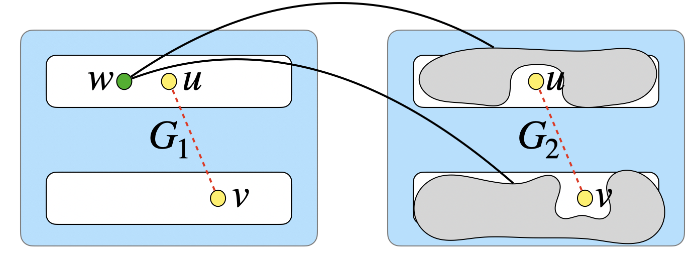
Figure 1: Alice’s input is $G_{1}$ and $G_{2}$ which are copies of the same random bipartite graph $G$. Bob’s input connects every vertex other than copies of $u$ and $v$ to each other. If we pick a vertex $w$ in the left to join the MIS, only vertices $u$ and $v$ in the right remain to join the MIS (the figure only shows some of $w$’s edges).

We can now do a round elimination to prove the lower bound. Think of the $0$-round “hard” problem as finding the MIS of a graph on a pair of vertices which may or may not be connected. The $1$-round hard problem above consists of $\Theta(n^{2})$ copies of this problem, with Bob’s input making exactly one of them, corresponding to the pair $\left\{u,v\right\}$, the special one; for the players to solve this $0$-round problem, Alice should have communicated enough information about $\left\{u,v\right\}$, which is not possible with $o(n^{2})$ size messages, given Alice does not know which of the $\Theta(n^{2})$ instances is special.

Beyond one-round lower bounds.

Suppose we want to extend this approach beyond a single round. We can use the same approach of using two identical copies of the same base graph for Alice and give Bob an input that connects these copies. Instead of a random graph however, we need Alice’s base graph to be a collection of independent copies of the $1$-round hard instances. Here, ‘independent’ copies not only mean in a probabilistic sense, but also in a graph-theoretic sense: the edges of one instance should not appear between vertices of another as otherwise the instances become “corrupted”, namely, they are no longer necessarily hard $1$-round instances. On top of this, we also need these instances to be quite large, so that a $1$-round lower bound for them incurs a significant communication cost in terms of the entire graph size (this is not a problem for the $1$-round case as a $0$-round protocol cannot have any communication no matter the input size).

A bit more specifically, to make this strategy work even for just a two-round $n^{1+\varepsilon}$ communication lower bound, for any constant $\varepsilon>0$, we need Alice’s base graph to have the following properties:

1. It must contain $(n^{1+\varepsilon})$ $1$-round instances so Alice cannot reveal too much about a random instance;

2. Each $1$-round instance needs to have $(n^{(1+\varepsilon)/2})$ vertices so that the quadratic $1$-round lower bound implies that the second round of the protocol needs $(n^{(1+\varepsilon)/2})^{2}=n^{1+\varepsilon}$ communication;

3. The instances cannot have edges between each others’ vertices so as not to “corrupt” one another.

Given that one-round instances have quadratic number of edges, satisfying all these constraints means having a base graph on $n$ vertices with $n^{2+2\varepsilon}$ edges or even pairs of vertices!

This highlights an inherent difficulty (basically, impossibility) of implementing this natural type of round elimination argument for proving communication lower bounds on graphs. In fact, almost all prior round-sensitive communication lower bounds on graphs (which are super linear in $n$) rely on more complicated arguments. For instance, the recent lower bounds in [AR20, CKP⁺21a, A22, AS23] require proving a lower bound for much harder intermediate problems to be able to carry out the inductive argument (e.g., see permutation hiding generators in [CKP⁺21a, AS23]; see also [A23] for a summary of these recent advances). The only exception is the very recent work of [KN24] that shows how to extend a similar one-round lower bound approach (but, for the matching problem in [GKK12]) to two-rounds, and prove a two-pass semi-streaming lower bound for approximate matching (we mention similarities and differences of these two approaches throughout this section).

2.2 Our Actual Lower Bound Approach: Hierarchical Embeddings

Even though the above approach seems quite hopeless, we show how to actually implement it modulo a crucial twist: we will not only start with many hard instances of the $(r-1)$-round problem in our $r$-round instance, but we will get the players to also solve many of these instances in the subsequent rounds (this is inspired by the aforementioned two-round lower bound of [KN24]). Specifically, we have $q\cdot p$ “hard” $(r-1)$-round sub-instances $\left\{I_{i,j}\right\}_{i\in[q],j\in[p]}$, each on $b$ vertices for some large parameters $q$, $p$, and $b$ as a function of $n$. These instances are again created based on a single base graph which is copied twice and given to the players; they are then connected via a clique structure, which identifies a sub-instance group $I_{t,*}:=I_{t,1},\ldots,I_{t,p}$ for a random chosen $t\in[q]$ as special instances. Restricting ourselves again to a two-round $n^{1+\varepsilon}$-communication lower bound, what we need from this base graph is the following:

1. We need $q\cdot p=n^{1+\varepsilon}$ so Alice’s first message does not reveal too much information;

2. We also need $p\cdot b^{2}=n^{1+\varepsilon}$ so Bob’s message cannot solve all $p$ special instances (each on $b$ vertices admitting a $1$-round $\Omega(b^{2})$-communication lower bound) in the second round;

3. Inducedness property: None of $q\cdot p$ sub-instances can have an edge between vertices of another sub-instance so as to not “corrupt” one another. Also, each sub-instance group $I_{i,*}$ for $i\in[q]$ should be vertex disjoint so that finding an MIS of their vertices requires solving all sub-instances.

Satisfying these constraints requires having a base graph on $n$ vertices with $q\cdot p\cdot b^{2}$ vertex-pairs. If we could set $p\approx q\approx n/b$, then, at least we will pass the basic test of “vertex-pair counting”. This in turn gives us a base graph with $\approx n^{2}/b^{2}$ sub-instances among which $\approx n/b$ are special (each admitting a 1-round $\Omega(b^{2})$-communication lower bound). Optimizing the parameters by setting $n^{2}/b^{2}=(n/b)\cdot b^{2}=n^{1+\varepsilon}$, implies that we can hope for obtaining an $\approx n^{4/3}$ lower bound (for $b\approx n^{1/3}$) for two-round algorithms this way.

Remark 1.

This is precisely the tradeoff achieved by the protocols for MIS in [ACG⁺15, GGK⁺18] in two rounds. In the first round, they sample $n/b$ vertices and send all their edges in $n^{2}/b^{2}$ communication, compute their MIS, and remove their neighbors. They prove that this reduces the maximum degree of remaining vertices to $\approx b$ only, and so in the next round they can send the remaining edges in $\approx n\cdot b$ communication and compute an MIS. This approach allows us to mimic the same exact tradeoffs for the lower bound for any number of passes.

Let us see how a base graph with these parameters should look like, especially given that the third requirement is quite strict: the induced subgraph of the base graph on vertices of $I_{i,*}$ for $i\in[q]$, should be a vertex-disjoint union of graphs in $I_{i,*}$, see Figure 2.

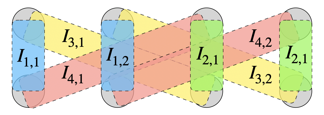
Figure 2: An illustration of the base graphs discussed above. Here $q=4$ and $p=2$ and each box denotes a single sub-instance (with different colors for different $I_{i,*}$ for $i\in[4]$). There are no edges between vertices of $I_{i,*}$ except for edges of the same sub-instances, which themselves are vertex-disjoint. While the figure may suggest sub-instances as being bipartite graphs, that crucially cannot be true in the actual construction.

Combinatorial considerations.

Do such graphs even exist? Notice that inserting each group of sub-instances $I_{i,*}$ adds $p\cdot b^{2}\approx n\cdot b$ edges to the graph, but prohibits roughly $\approx p^{2}\cdot b^{2}\approx n^{2}$ vertex-pairs to ever appear as an edge in the graph (to ensure the inducedness property, vertices of a single sub-instance in $I_{i,*}$ cannot have edges to any of the remaining $(p-1)\cdot b$ vertices of the sub-instances of $I_{i,*}$). This seems to suggest that by the time we have added barely a super-constant number of sub-instance groups $I_{i,*}$, i.e., when $q$ is becoming super-constant and way before $q\approx n/b$, we will run out of edges and thus cannot continue. In other words, these graphs can only be sparse, and are hence not at all suitable for a super-linear-in-$n$ lower bound.

The above argument however is flawed because the vertex-pairs prohibited by these sub-instance groups can be shared among each other (as opposed to edges that cannot be shared). Indeed, succinctly stated, the base graphs for $r$-round instances are disjoint collections of induced subgraphs that are vertex-disjoint unions of hard $(r-1)$-round instances. This definition is reminiscent of Ruzsa-Szemerédi (RS) graphs [RS78]: these are graphs that consist of many disjoint induced matchings. The same “flawed reasoning” also applies to RS graphs and yet, in reality, they can become quite dense, with even ${{n}\choose{2}}-o(n^{2})$ edges and induced matchings of size $p=n^{1-o(1)}$ [AMS12].

The difference with RS graphs for us is that we need induced subgraphs that are much more complicated than matchings. One of our main contributions is an almost-optimal construction of these graphs for a large family of induced subgraphs (which can be any $n^{o(1)}$-colorable graph). Our construction relies on two separate ingredients: $(i)$ another family of extremal graphs referred to as “directed graphs requiring large number of shortcuts” [Hes03] or “graphs with many long disjoint shortest paths” [AB16] studied extensively in the context of hopsets and spanners lower bounds (see, e.g., [CE06, HP21, BH22, LWWX22, WXX23]); and, $(ii)$ a graph product, which we call embedding product, that allows for “packing” a large number of complex induced subgraphs inside a single graph of part $(i)$. See Section 2.3 for a detailed overview.

Information-theoretic considerations.

We have so far focused on the combinatorial aspects of our approach. The next step are the information theoretic arguments for proving the lower bound. Here, our work can be seen as generalizing and unifying two previously disjoint sets of techniques for proving round-sensitive communication lower bounds (discussed in more detail in Section 2.4):

• The round elimination arguments of [ANRW15] and [AKZ22] for approximate matchings and MIS, respectively, for quite different and “algorithmically weaker” models of communication (e.g., one cannot implement the MIS algorithms of [ACG⁺15, GGK⁺18] in these models). These lower bounds in particular work with a much larger number of players (proportional to vertices in the graph) and do not allow interaction between the players in each single round.

• The line of work, starting from [GKK12], that use RS graphs for proving semi-streaming lower bounds and in particular, a very recent result of [KN24] that proves a two-pass lower bound for the matching problem. These prior works typically rely on different reductions to various communication problems—which are often different from the original underlying problem—say, Index in [GKK12] and HiddenStrings in [KN24]. Our approach, on the other hand, takes advantage of a “self-reducibility” property of the problem which allows for implementing a round elimination argument over multiple passes/rounds.

The hierarchical embedding technique.

Let us now reiterate how our hierarchical embedding technique works at a high level. For technical reasons, our $r$-round lower bound will be against $(r+1)$-party (number-in-hand) protocols instead of just two parties.

We pick $q_{r}\cdot p_{r}$ hard $(r-1)$-round sub-instances with $r$-players in a set $\mathcal{I}:=\left\{I_{i,j}\right\}_{i\in[q_{r}],j\in[p_{r}]}$, each on $b_{r}$ vertices, for parameters $q_{r},p_{r}$, and $b_{r}$ to be determined soon.

We use our combinatorial constructions to embed all these instances into a single base graph $G$ with the inducedness property mentioned earlier (and then copied identically twice as before). For every $a\in[r]$, the input of the $a^{\textnormal{th}}$ player in the $r$-round instance is the collection of the inputs of all $a^{\textnormal{th}}$ players in sub-instances in $\mathcal{I}$. The $(r+1)^{\textnormal{th}}$ player in the $r$-round instance gets a clique-subgraph as before that “points” to one of the sub-instance groups $I_{t,*}$ for a random $t\in[q_{r}]$.

This way, the input consists of a hierarchy of different-round instances of the problem, and the players have to solve multiple root-to-leaf paths of this hierarchy to obtain a solution to the entire input as well. Our round elimination argument then shows that the first round of the protocol cannot reveal enough information about the special sub-instance group to allow solving all of them in the remaining $(r-1)$ rounds. See Figure 3 for an illustration.

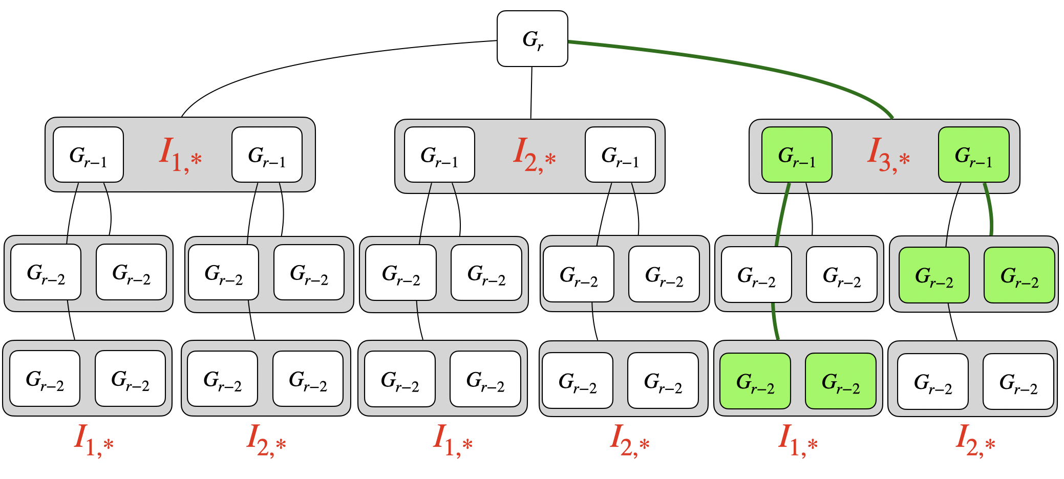
(a) The hierarchical instances form a conceptual tree, and the players need to “solve” certain root-to-leaf paths.

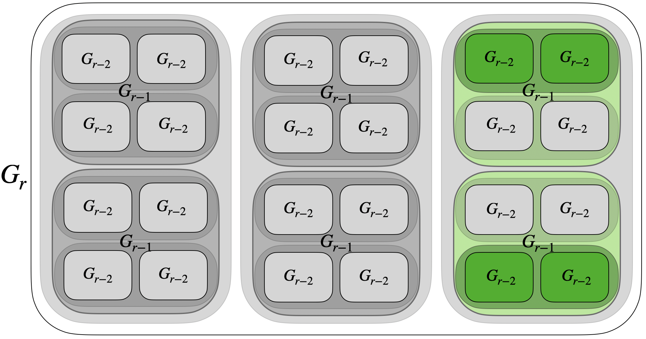
(b) The input graph is also a hierarchy of induced subgraphs (this figure shows these graphs in a vertex-disjoint way for simplicity of drawing, but in reality, vertices of these graphs are highly “tangled”).

Figure 3: An illustration of the hierarchical embedding technique.

Finally, the choice of the parameters $q_{r},p_{r}$ and $b_{r}$ is as follows. Let $C(n,r)$ denote the lower bound on the communication cost we hope to prove for $r$-round protocols on $n$-vertex graphs. Then,

$$q_{r}\cdot p_{r}\approx C(n,r):\text{so players cannot reveal much about $p_{r}$ special sub-instances in the first round}$$

$$p_{r}\cdot C(b_{r},r-1)\approx C(n,r):\text{so solving the $p_{r}$ special $b_{r}$-size sub-instances in $r-1$ rounds is hard}.$$

Picking these parameters optimally, while accounting for the restrictions imposed by the combinatorial construction (and an $n^{o(1)}$-“loss” on size of these graphs compared to absolute best-imaginable bounds), gives us our $\approx n^{1+1/(2^{r}-1)}$ communication lower bound for $r$-round $(r+1)$-party protocols.

Remark 2.

As should be clear from this discussion, our hierarchical embedding technique is quite general and is not particularly tailored to the MIS problem. Hence, it seems quite plausible to extend this approach to various other graph problems as well, making hierarchical embeddings a general technique for proving multi-pass graph streaming lower bounds.

2.3 Combinatorial Part: Dense Graphs with Many Induced Subgraphs

We now discuss the construction of our base graphs for our hierarchical embeddings. Recall that we need an $n$-vertex graph $G$ with $q\approx n/b$ subgraph groups $\left\{H_{i,*}\right\}_{i\in[q]}$, each with $p\approx n/b$ vertex-disjoint subgraphs $\left\{H_{i,1},\ldots,H_{i,p}\right\}_{i\in[q]}$ on $b$ vertices each. In addition, the inducedness property requires that there are no other edges between the vertices of each subgraph group (other than the edges of the subgraphs themselves). Refer back to Figure 2 from earlier for an illustration.

Our starting point is the recent RS-graph based constructions in streaming lower bounds in [AS23, KN24]. In particular, [AS23] created a graph with “high entropy permutations” in place of edges of RS graphs and [KN24] took this even further with a graph that has many “small” RS graphs embedded inside one larger RS graph (roughly speaking, by changing each edge of the outer RS graph, with a copy of the inner RS graph). These constructions, however, are still insufficient for us as they can support quite limited “inner” graphs, while our hierarchical embeddings require a graph consisting of highly complex subgraphs corresponding to hard instances of MIS with one less round. For instance, both constructions in [AS23, KN24] inherently can only support bipartite inner graphs while our hard instances definitely cannot be bipartite as finding MIS of bipartite graphs is easy with $\approx n$ communication in one round.

Our constructions work with an outer graph, which, instead of induced matchings in RS graphs, contains many Unique Path Collections (UPCs) that can almost be seen as “stretching” an induced matching (a collection of paths of length $1$), to longer paths (see 4.3 for the formal definition and Figures 4 and 7 for illustrations). The ‘almost’ part however is due to a subtle difference: the property of UPCs goes beyond only their induced subgraphs – instead, these paths are not only induced on their vertices, but also are the unique shortest path between their endpoints even if one uses outside vertices. See Figure 4 for an example.

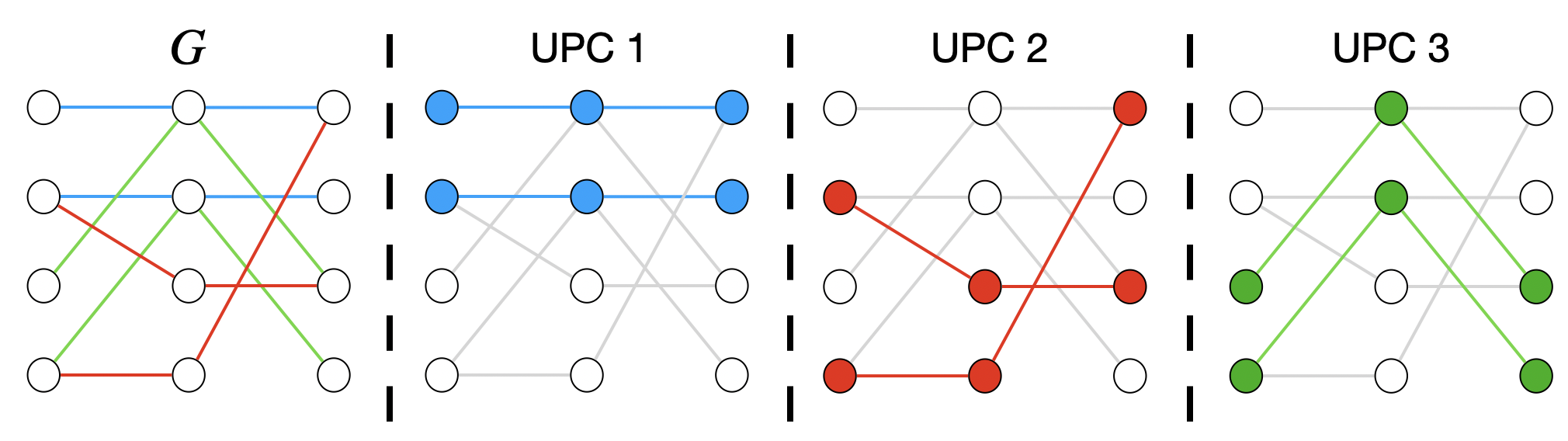
Figure 4: An example of UPCs in the graph $G$ on the left. In each UPC, there is no path of length $2$ from a starting vertex to an end vertex unless the path belongs to the UPC itself.

Such outer graphs have been already studied extensively in the context of shortcutting sets and spanners; see, e.g.,  [Hes03, AB16, CE06, HP21, BH22, LWWX22, WXX23] and references therein. For our purpose, we need a slight variation that follows from the approach in [AB16], which is itself based on the original RS graph constructions in [RS78] (the variation allows for “packing” many paths together in a UPC, as opposed to the path-wise guarantee of prior work). Nevertheless, it appears that the way we use these graphs is completely different from prior work. We are also not aware of any prior applications of these graphs to streaming or communication lower bounds, or to the maximal independent set problem in any other computational model.

Having obtained these outer graphs, our embedding product works by replacing, for every $i\in[q]$, each path in the $i^{\textnormal{th}}$ UPC of these graphs with the subgraphs in $H_{i,*}$ that we would like to have in our base graph. The only requirement we need from subgraphs $\left\{H_{i,j}\right\}_{i,j}$ is that they should have a small chromatic number; in particular, as long as they are $k$-colorable graphs, we can also embed them in UPCs with paths of length $k-1$ by mapping each of their color classes to one of the vertices of the path in a careful way. The strong guarantee of our outer graphs can then be used to argue that these $k$-colorable graphs cannot have inserted an edge between vertices of each other (i.e., break the inducedness property), as such an edge can be traced backed to a “shortcutting path” in the outer graph which cannot exist. See Figure 5 for an illustration.

Figure 5: If the solid (red) edge between $u$ and $v$ is inserted by any other $k$-colorable graph $H_{i,j}$ for $i\neq 1$, we will also find a shortcut between “outer” versions of $u$ and $v$, which cannot exist in the outer graph.

Finally, in our application to MIS, we start with $2$-colorable graphs as our base case instances that are hard for $0$-round protocols. The identical copying plus adding a clique between some parts of the two copies that we mentioned earlier, with some modifications, leads to a $4$-colorable hard instance for $1$-round protocols. Following the same pattern thus leads to $2^{r+1}$-colorable graphs for $r$-round protocols. Our construction allows for setting $q\approx p\approx n^{1-o(1)}$ for embedding any $n^{o(1)}$-colorable graphs, and since we will only need to continue the lower bound for $r\approx\log\log{n}$ rounds, we will have more than enough room to carry out the entire plan.

2.4 Information-Theoretic Part: Round Elimination via Direct-Sum

We will now discuss the information-theoretic parts of our lower bound. The combinatorial parts of our lower bound gives us a quite strong boost here: we can now solely focus on the ability of the protocols in “traversing” the hierarchical tree of instances we discussed earlier (see Figure 3), without worrying about any interference between underlying instances of the problem (there is none owing to the inducedness property of our construction). In other words, the communication lower bound here is practically independent of the MIS problem and is essentially (although not quite) only about the abstract problem of traversing the hierarchical tree:

• The first $r$ players receive $q_{r}\cdot p_{r}$ “hard” $(r-1)$-round sub-instances $\mathcal{I}:=\left\{I_{i,j}\mid i\in[q_{r}],j\in[p_{r}]\right\}$; the last player receives an index $t\in[q_{r}]$;

• The goal for the players is to solve all special sub-instances of $I_{t,*}$ in $r$ rounds.

This problem is similar in spirit to the tree-pointer jumping problem of [CCM08]. The crucial difference is that tree-pointer jumping only has one special instance per level (think of $p_{r}=1$ above), whereas for us, we need the players to solve many “small” sub-instances—which, individually, are not hard to solve within the budget of even the $(r-1)$-round protocols (this is precisely our deviation from the ideal-type lower bounds to our actual lower bound). A similar problem was also very recently introduced by [KN24] only for $2$-round protocols as their HiddenStrings problem. However, the techniques in [KN24]—based on the two-way communication complexity of the Index problem [JRS09]—are inherently only for $2$-round protocols and do not generalize beyond.

Our second technical contribution is a lower bound for this problem (in a bit less abstract form).

An intuitive “proof”.

Suppose we have a protocol $\pi$ with $s=o(p_{r}\cdot q_{r})$ communication on the distribution $\mathcal{G}_{r}$ of $r$-round instances. We can first show that, in its first round, $\pi$ can only reveal $O(s/q_{r})=o(p_{r})$ bits in total about all instances in $I_{t,*}$ (as these are an unknown $1/q_{r}$ fraction of the inputs in $\mathcal{I}$). This means that on average $\pi$ has only revealed $o(1)$ bits about any one instance $I_{t,j}$ for $j\in[p_{r}]$. Thus, in the remaining $r-1$ rounds, it needs to solve $p_{r}$ copies of the $(r-1)$-round problem, where each copy, on average, is only $o(1)$ statistical distance away from the hard $(r-1)$-round distribution $\mathcal{G}_{r-1}$. This second problem has a flavor of a direct-sum result. Hence, using a direct-sum style argument (say, as in [BBCR10]), we should also be able to say that in the remaining $(r-1)$ rounds, $\pi$ needs to communicate $p_{r}$ times the communication cost of solving one $(r-1)$-round hard instance. This gives us the tradeoff stated at the very end of Section 2.2.

Unfortunately, making this intuition precise is hindered by the fact that in this direct-sum scenario, the $p_{r}$ $(r-1)$-round instances, in addition to their marginal deviation of $o(1)$ from $\mathcal{G}_{r-1}$, also have become correlated with each other for a total of $o(p_{r})$ bits. In other words, the first message of $\pi$ can also change their joint distribution by revealing $o(p_{r})$ bits about them collectively. In general, one cannot hope for a direct-sum result to hold over such non-independent instances.

Our actual proof.

To tackle this obstacle, we apply an information complexity direct-sum to the previous round elimination arguments of [ANRW15, AKZ22]. Specifically, we show how to obtain a $(r-1)$-round protocol $\pi^{\prime}$ for a single hard $(r-1)$-round instance using the protocol $\pi$: High level description of the protocol $\pi^{\prime}$ for $I_{r-1}\sim\mathcal{G}_{r-1}$: 1. Sampling step: Sample the first message $\Pi_{1}$ of $\pi$ and a family of sub-instances $\mathcal{I}$ from $\mathcal{G}_{r}$, i.e., $(\Pi_{1},\mathcal{I})\sim\mathcal{G}_{r}$. Then, sample $k\in[p_{r}]$ uniformly at random and replace $I_{t,k}$ in $\mathcal{I}$ with the input instance $I_{r-1}$ (where $t$ is the index of the special sub-instance group of $\mathcal{I}$). 2. Simulation step: Run the protocol $\pi$ on the modified $\mathcal{I}$ from its second round onwards and output the answer of $\pi$ on the special sub-instance $I_{t,k}$.

The analysis consists of two parts, one for each step of the protocol. The first part shows how the players can sample the joint variables $(\Pi_{1},\mathcal{I})$ and embed $I_{r-1}$ inside $\mathcal{I}$—which crucially is independent of $\Pi_{1}$ in this sampling, although it should not be in the distribution of by $\pi$—using a distribution that is close to $\mathcal{G}_{r}\mid I_{i,j}=I_{r-1}$. This sampling is inspired by [ANRW15, AKZ22] with various modifications to account for the considerable differences between the two communication models. Proving this part is based on a similar argument as in the intuitive “proof” above that says that the marginal distribution of $I_{i,j}$ is not affected that much by the first-round message $\Pi_{1}$.

The second part of the argument, however, deviates entirely from [ANRW15, AKZ22], because in their communication model, the new protocol $\pi^{\prime}$ already has the desired communication cost for an $(r-1)$-round protocol (given their focus on maximum message-size per vertex of the graph); thus, their arguments finish at this point. However, for us, the protocol $\pi^{\prime}$ has the same communication cost as $\pi$ even though it is being run on a much smaller instance. Hence, there is no contradiction that $\pi^{\prime}$ can solve $\mathcal{G}_{r-1}$ in $(r-1)$ rounds as its communication cost is way above the bar anyway.

To handle this part, we instead work with the information cost of the protocols (in place of their communication cost) for a natural multi-party generalization of two-party external information cost in [BBCR10] (see Section 3.2 for the definition). Our approach is then to show that even though $\pi^{\prime}$ may communicate as much as $\pi$, its information cost is a factor $1/p_{r}$ smaller than the information cost of $\pi$. This is because $I_{r-1}$ is embedded in one of the $p_{r}$-many special sub-instances randomly whose identity is hidden to the protocol $\pi$. But, this creates another challenge: information cost, unlike communication, is a function of the underlying distribution, and in $\pi^{\prime}$, the distribution of the inputs that $\pi$ is simulated on is not the original distribution $\mathcal{G}_{r}$, only statistically close to it. Thus, even though we know that $\pi$ has a low information cost on $\mathcal{G}_{r}$, we cannot guarantee it also has a low information cost in the simulation step and conclude that $\pi^{\prime}$ has a low information cost.

The challenge outlined above is not unique to our problem and has been studied before also, e.g., for direct-product results in [BRWY13b, BRWY13a, BW15] but typically for internal information cost and two-party protocols. For our purpose, we use a message compression technique due to [HJMR07] (see also [BG14]) to reduce the communication cost of the protocol $\pi$ in the simulation step down to its information content. This leads to some minimal loss in the parameters that can be easily handled in our setting. But now, the change in the underlying distribution of the simulation step cannot affect the communication cost, which allows us to obtain a too-good-to-be-true protocol $\pi^{\prime}$ for $\mathcal{G}_{r-1}$, which leads to our desired contradiction.

This concludes our overview. In the rest of the paper, we formalize the ideas and approaches discussed in this section and prove 1 and 2 formally.

3 Preliminaries

Notation.

For any $t\geqslant 1$, define $[t]:=\left\{1,\ldots,t\right\}$. Some times, for a clarity of exposition, we may write $(a)\uparrow(b)$ to denote $a^{b}$. For any tuple $(x_{1},\ldots,x_{t})$ and $i\in[t]$, we define $x_{<i}:=(x_{1},\ldots,x_{i-1})$. We define $x_{>i}$ and $x_{-i}$, analogously. For a set of tuples $\left\{(x,y)\mid x\in X,y\in Y\right\}$ for some sets $X$ and $Y$, and $x\in X$, we define $(x,*):=\left\{(x,y)\mid y\in Y\right\}$; we define $(*,y)$ for $y\in Y$ analogously.

When there is room for confusion, we use sans-serif letters for random variables (e.g. ${\mathsf{A}}$) and normal letters for their realizations (e.g. $A$). We use $\textnormal{dist}({\mathsf{A}})$ and $\textnormal{\text{supp}}({\mathsf{A}})$ to denote the distribution of ${\mathsf{A}}$ and its support, respectively.

For random variables ${\mathsf{A}},{\mathsf{B}}$, we use $\mathbb{H}({\mathsf{A}})$ to denote the Shannon entropy and $\mathbb{I}({\mathsf{A}}\,;{\mathsf{B}})$ to denote the mutual information. For two distributions $\mu$ and $\nu$ on the same support, $\|\mu-\nu\|_{\mathrm{tvd}}$ denotes their total variation distance and $\mathbb{D}(\mu~{}||~{}\nu)$ is their KL-divergence. Appendix A contains the definitions of these notions and standard information theory facts that we use in this paper.

3.1 (Multi-Party) Communication Complexity

We work in the standard multi-party number-in-hand communication model; we provide some basic definitions here and refer the interested reader to the excellent textbooks [KN97, RY20] on communication complexity for more details.

There are $k\geqslant 1$ players $P_{1},\ldots,P_{k}$ in this model who receive a partition of the edges of an input graph $G=(V,E)$. The players follow a protocol $\pi$ to solve a given problem on $G$, say, finding an MIS. They have access to a shared tape of randomness, referred to as public randomness, in addition to their own private randomness. In each round, $P_{1}$ writes a message on a board visible to all parties, followed by $P_{2}$, all the way to $P_{k}$. Each message can only depend on the private input of the sender, content of the blackboard, public randomness, and private randomness of the sender. At the end of the last round, the last player $P_{k}$ writes the answer to the blackboard.

Definition 3.1.

For any protocol $\pi$, the communication cost of $\pi$, denoted by $\textsc{CC}(\pi)$, is defined as the worst-case (maximum) length of messages, measured in bits, communicated by all players on any input. We assume that all transcripts, i.e., the set of all messages written onto the blackboard, in $\pi$ have the same worst-case length (by padding).

Communication complexity and streaming.

The following standard result—dating back (at the very least) to the seminal paper of [AMS96] that introduced the streaming model—relates communication cost of protocols and space of streaming algorithms.

Proposition 3.2 (cf. [AMS96]).

For any $p\geqslant 1,s\geqslant 1$, and $\delta\in(0,1)$, suppose there is a $p$-pass $s$-space $\delta$-error streaming algorithm $A$ for some problem $\mathbb{P}$. Then, for any integer $k\geqslant 1$, there also exists a $k$-party protocol $\pi$ with $p$ rounds, communication cost $\textsc{CC}(\pi)\leqslant p\cdot k\cdot s$, and error probability at most $\delta$, for the same problem $\mathbb{P}$.

Proof.

Consider the stream $\sigma=\sigma_{1}\circ\cdots\circ\sigma_{k}$ where $\sigma_{i}$ is the input to the player $P_{i}$ in $\pi$ (ordered arbitrarily in the stream). Player $P_{1}$ runs $A$ on $\sigma_{1}$ and writes the memory content on the board, which allows player $P_{2}$ to continue running $A$ on $\sigma_{2}$, and so on and so forth. This allows the players to run one pass of $A$ using communication cost at most $k\cdot s$. The players can continue this in $p$ rounds, faithfully simulating the $p$ passes of the algorithm, and at the end $P_{k}$ can read the answer of $A$ from the memory and outputs it on the blackboard.

This way, $\pi$ will have the same probability of success as $A$, uses at most $p\cdot k\cdot s$ communication and $p$ rounds of communication.       

Proposition 3.2 allows us to translate communication lower bounds into streaming lower bounds. In particular, this result reduces proving 1 to proving 2.

3.2 Information Cost and Message Compression

We also work with the notion of information cost of protocols that originated in [CSWY01] and has since found numerous applications (see, e.g. [Wei15] for an excellent survey of this topic).

There are various definitions of information cost that have been considered depending on the application. The definition we use—which is a natural multi-party variant of the standard external information cost [BBCR10]—is best suited for our application.

Definition 3.3.

For any multi-party protocol $\pi$ whose inputs are distributed according to the distribution $\mu$, the (external) information cost is defined as: $$\textsc{IC}(\pi,\mu):=\mathbb{I}({\mathsf{G}}\,;{\mathsf{\Pi}}\mid{\mathsf{R}}),$$ where ${\mathsf{G}}$ denotes the random variable for the input graph sampled from $\mu$, ${\mathsf{\Pi}}$ denotes the set of all messages written on the board, and ${\mathsf{R}}$ is the public randomness.

In words, multi-party external information cost measures the information revealed by the entire protocol about the entire graph to an external observer. The following result follows from [BBCR10].

Proposition 3.4 (cf. [BBCR10]).

For any multi-party protocol $\pi$ on any input distribution $\mu$,

$$\textsc{IC}(\pi,\mu)\leqslant\textsc{CC}(\pi).$$

Proof.

We have,

$$\textsc{IC}(\pi,\mu)\underset{\textnormal{(1)}}{=}\mathbb{I}({\mathsf{G}}\,;{\mathsf{\Pi}}\mid{\mathsf{R}})\underset{\textnormal{(2)}}{=}\mathbb{H}({\mathsf{\Pi}}\mid{\mathsf{R}})-\mathbb{H}({\mathsf{\Pi}}\mid{\mathsf{G}},{\mathsf{R}})\underset{\textnormal{(3)}}{\leqslant}\mathbb{H}({\mathsf{\Pi}}\mid{\mathsf{R}})\underset{\textnormal{(4)}}{\leqslant}\mathbb{H}({\mathsf{\Pi}})\underset{\textnormal{(5)}}{\leqslant}\log{\left|{\textnormal{\text{supp}}({\mathsf{\Pi}})}\right|}\underset{\textnormal{(6)}}{=}\textsc{CC}(\pi);$$

here, $(1)$ is by the definition information cost, $(2)$ is by the definition of mutual information, (3) is by the non-negativity of entropy (A.1-(1)), (4) is because conditioning can only reduce the entropy (A.1-(3)), (5) is because uniform distribution has the highest entropy (A.1-(1)), and (6) is by the definition of worst-case communication cost.       

Message compression.

We use message compression to reduce communication cost of protocols close to their information cost in certain settings. The following result is due to [HJMR07] which was further strengthened slightly in [BG14]. We follow the textbook presentation in [RY20].

Proposition 3.5 (c.f.[RY20, Theorem 7.6]).

Suppose Alice knows two distributions $\mathcal{A},\mathcal{B}$ over the same set ${U}$ and Bob only knows $\mathcal{B}$. Then, there is a protocol for Alice and Bob to sample an element according to $\mathcal{A}$ by Alice sending a single message of size

$$\mathbb{D}(\mathcal{A}~{}||~{}\mathcal{B})+2\log(1+\mathbb{D}(\mathcal{A}~{}||~{}\mathcal{B}))+O(1)$$ (1)

bits in expectation. This protocol has no error.

We note that somewhat weaker bounds on the KL-Divergence in Eq 1 already suffice for our purposes. Thus, to simplify the exposition, we use,

$$\mathbb{D}(\mathcal{A}~{}||~{}\mathcal{B})+2\log(1+\mathbb{D}(\mathcal{A}~{}||~{}\mathcal{B}))+O(1) \leqslant\mathbb{D}(\mathcal{A}~{}||~{}\mathcal{B})+10\mathbb{D}(\mathcal{A}~{}||~{}\mathcal{B})+O(1) \log(1+x)\leqslant 5x x\geqslant 0$$ (as for every )

$$\leqslant c_{\textnormal{comp}}\cdot\left(\mathbb{D}(\mathcal{A}~{}||~{}\mathcal{B})+1\right),$$ (2)

for some absolute constant $c_{\textnormal{comp}}\geqslant 1$ that we use from now on in our proofs.

4 Disjoint-Unique-Paths Graphs and Embedding Products

Our lower bound for MIS relies on two graph-theoretic ingredients: $(i)$ an extremal family of graphs which can be seen as a generalization of RS graphs [RS78], and $(ii)$ a graph product which we call the embedding product for this particular family of graphs. We now define these constructions and establish their key properties. To continue, we need the following basic definitions (see Figure 6).

Definition 4.1.

For any $n,k\geqslant 1$, a graph $G=(V,E)$ is called a $(n,k)$-layered graph if there exists an equipartition of $V$ into $k$ independent sets $(V_{1},V_{2},\ldots,V_{k})$ of size $n/k$ each, referred to as layers of $G$. We additionally say that $G$ is a strictly-layered graph if all edges of $G$ are between consecutive layers.

Definition 4.2.

For any $n,k\geqslant 1$, a path $P$ in an $(n,k)$-strictly-layered graph $G$ is called a layered path if it has edges between consecutive layers and exactly one vertex per layer. For any layered path $P$, we define $\textnormal{{start}}(P)$ as the vertex of $P$ in the layer $V_{1}$ of $G$ and $\textnormal{{final}}(P)$ as the vertex of $P$ in the layer $V_{k}$.

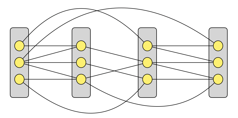
(a) A $(12,4)$-layered graph.

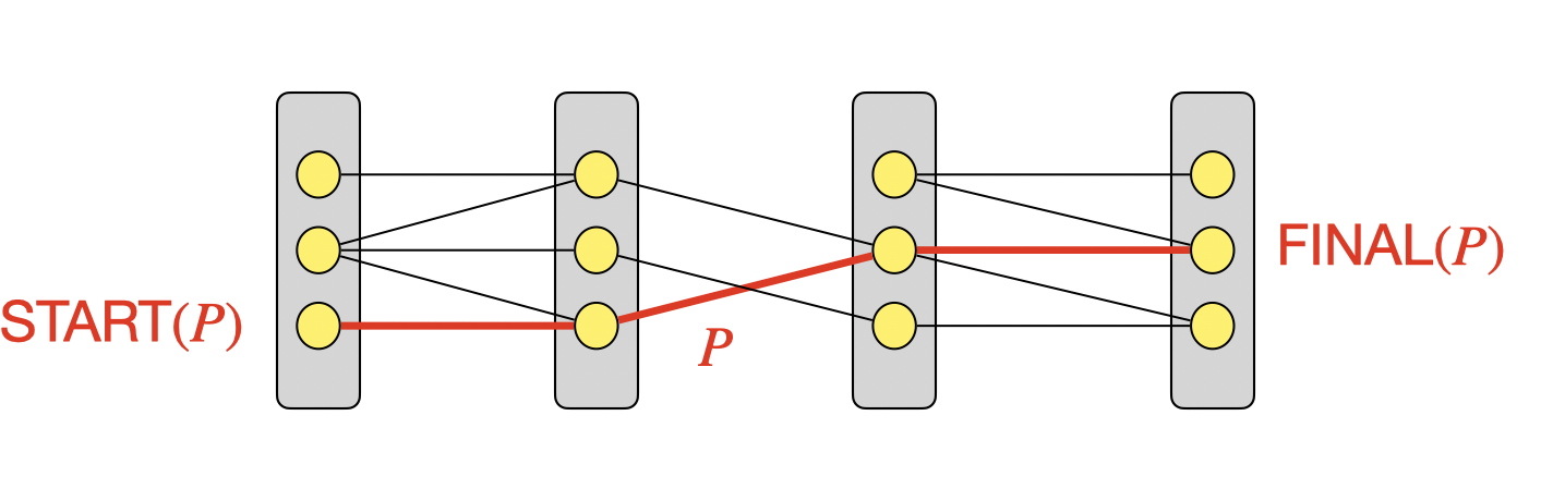
(b) A $(12,4)$-strictly-layered graph and a layered path inside it.

Figure 6: An illustration of layered graphs and strictly-layered graphs with a layered path.

4.1 Disjoint-Unique-Paths (DUP) Graphs

The following definition captures the key concept we need from our extremal graphs.

Definition 4.3.

A set of paths $\mathcal{P}$ in a strictly-layered graph $G$ is called a unique path collection (UPC) iff $(i)$ $\mathcal{P}$ is a vertex-disjoint set of layered paths, and, $(ii)$ for any pair of vertices $s$ in $\textnormal{{start}}(\mathcal{P}):=\left\{\textnormal{{start}}(P)\mid P\in\mathcal{P}\right\}$ and $t$ in $\textnormal{{final}}(\mathcal{P}):=\left\{\textnormal{{final}}(P)\mid P\in\mathcal{P}\right\}$, the only layered path between $s$ and $t$ in the entire graph $G$ is a path in $\mathcal{P}$ (if one exists, $s$ and $t$ are the two ends of the same path $P\in\mathcal{P}$).

Figure 7: An illustration of a UPC in a strictly-layered graph. Neither the dashed red edges (between the vertices of different paths in a UPC) nor the edges of the solid red path (using outside vertices) are allowed.

See Figure 7 for an example of UPCs. We use UPCs to define our extremal graph family.

Definition 4.4.

For any $n,k,p,q\geqslant 1$, a $(p,q,k)$-disjoint-unique-paths (DUP) graph is a $(n,k+1)$-strictly-layered graph $G$ whose edges can be partitioned into $q$ UPCs $\mathcal{P}_{1},\ldots,\mathcal{P}_{q}$, each consisting of exactly $p$ layered paths $P_{i,1},\ldots,P_{i,p}\in\mathcal{P}_{i}$ for $i\in[q]$.

The following result shows the existence of $(p,q,k)$-DUP graphs with $p,q=n^{1-o(1)}$ (that is necessary for our application) and $k=\omega(\mbox{\rm poly}\!\log{(n)})$ (that is sufficient for our application). The existence of such results is a-priori surprising as UPCs of size $p$ are “locally sparse” and restrict many edges from appearing in the graph, and yet large $q$ implies that the graph is “globally dense”. Nevertheless, we can use the same ideas as they are used in the construction of RS graphs [RS78] or for ‘graphs with many long disjoint shortest paths’ in [AB16] to construct DUP graphs.

Proposition 4.5.

For any sufficiently large $n\in\mathbb{N}$ and any given $k\geqslant 1$ satisfying $k\leqslant 2^{(\log{n})^{1/4}}$, there exists a $(p,q,k)$-DUP graph on $n$ vertices with the following parameters for two absolute constants $\eta_{p},\eta_{q}>0$,

$$p=\frac{n}{\exp\left(\eta_{p}\cdot(\ln{n})^{3/4}\right)}\qquad\text{and}\qquad q=\frac{n}{\exp\left(\eta_{q}\cdot(\ln{n})^{3/4}\right)}.$$

Given that this result does not seem to have appeared in prior work, we provide a self-contained proof in Section 4.3, which may also provide some more intuition about these graphs.

4.2 Embedding Products

The next key ingredient of our construction is a graph product that treats DUP graphs as an “outer” graph and replace their entire paths in UPCs with different “inner” layered graphs (not necessarily strictly-layered ones). See Figure 8 for an illustration.

Definition 4.6.

Let $G_{\textsc{dup}}$ be a $(p,q,k)$-DUP graph on $n_{1}$ vertices and layers $U_{1},\ldots,U_{k+1}$ for some $p,q,k\geqslant 1$. Let $\mathcal{H}:=\left\{H_{i,j}\mid i\in[q],j\in[p]\right\}$ be a family of $(n_{2},k+1)$-layered graphs where all the graphs in $\mathcal{H}$ are on the same layers $W_{1},\ldots,W_{k+1}$ but may have different edges. We define the embedding of $\mathcal{H}$ into $G_{\textsc{dup}}$, denoted by $G:=\textnormal{{embed}}(\mathcal{H}\rightarrow G_{\textsc{dup}})$, as the following $((n_{1}\cdot n_{2})/(k+1),k+1)$-layered graph: • Vertices: We have layers $V_{1},\ldots,V_{k+1}$ where, for every $\ell\in[k+1]$, $V_{\ell}:=U_{\ell}\times W_{\ell}$; • Edges: For any layered path $P_{i,j}=(u_{1},u_{2},...,u_{k+1})$ of UPC $\mathcal{P}_{i}$ in $G_{\textsc{dup}}$ with $i\in[q]$ and $j\in[p]$, and any edge $(x,y)\in H_{i,j}$ between layers $W_{\ell_{x}}$ and $W_{\ell_{y}}$, we add an edge $e$ between $(u_{\ell_{x}},x)$ and $(u_{\ell_{y}},y)$ to $G$. We say that the edge $e$ is added w.r.t. the path $P_{i,j}$.

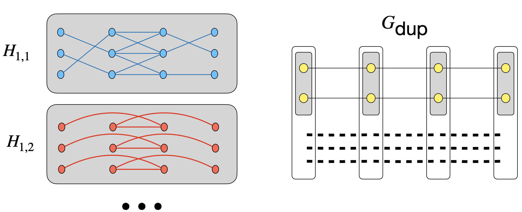
(a) A family $\mathcal{H}$ including $(12,4)$-layered graphs $H_{1,1}$ and $H_{1,2}$ (remaining graphs are unspecified) on the left and a DUP graph $G_{\textsc{dup}}$ with $p=2$, unspecified $q$, and $k=3$ on the right.

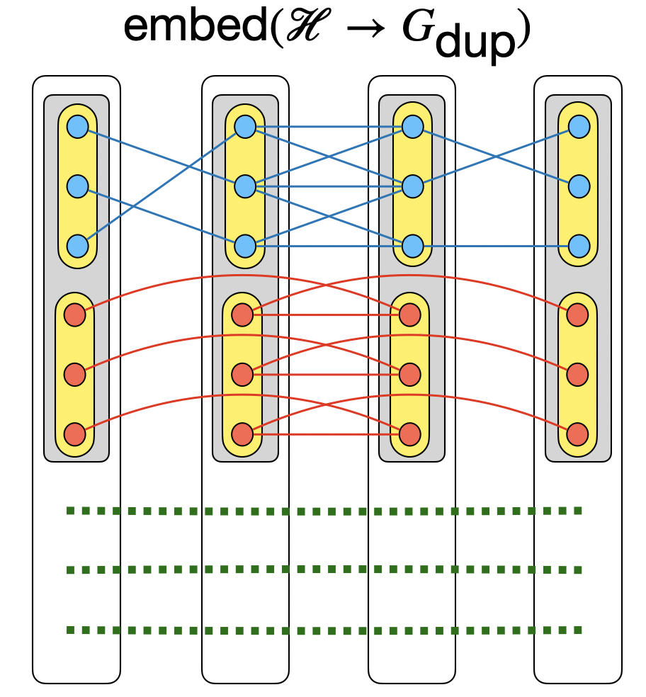
(b) The resulting layered graph as the embedding of $\mathcal{H}$ into $G_{\textsc{dup}}$ – the drawing only shows the effect of the embedding on one UPC of $G_{\textsc{dup}}$ and the remainder of the graph is unspecified.

Figure 8: An illustration of the embedding product. For simplicity of exposition, this figure only shows a part of the final graph obtained via embedding inside a single UPC of the DUP graph; in the actual construction, every UPC is replaced by an embedded graph.

The following lemma captures the main property of these embeddings.

Lemma 4.7.

Let $G_{\textsc{dup}}$ be a $(p,q,k)$-DUP graph for some $p,q,k\geqslant 1$, $\mathcal{H}:=\left\{H_{i,j}\mid i\in[q],j\in[p]\right\}$ be a family of layered graphs with size $p\cdot q$, and $G:=\textnormal{{embed}}(\mathcal{H}\rightarrow G_{\textsc{dup}})$. For any $i\in[q]$, the induced subgraph of $G$ on vertices corresponding to $\mathcal{P}_{i}$, i.e., $\left\{(v,*)\mid v\in P_{i,j}~{}\text{for some $P_{i,j}\in\mathcal{P}_{i}$}\right\}$, is a vertex-disjoint union of graphs $H_{i,j}$ for $j\in[p]$ in $\mathcal{H}$.

Before getting to the proof of Lemma 4.7, an important remark is in order. Recall that our layered graphs can have edges between any pairs of layers and not only consecutive ones. As such, to be able to establish the property in Lemma 4.7, we crucially rely on the fact that DUP graphs not only disallow any additional edges between vertices of a UPC, but in fact, no layered paths can connect them also even if the paths are using vertices outside the UPC. This is the key property of DUP graphs that is needed for our constructions.

Proof of Lemma 4.7.

For any $i\in[q]$, let $U_{i}:=\left\{(v,*)\mid v\in P_{i,j}~{}\text{for some $P_{i,j}\in\mathcal{P}_{i}$}\right\}$ denote the vertices of $G$ corresponding to the UPC $\mathcal{P}_{i}$. Let $G_{i}:=G[U_{i}]$ be the induced subgraph of $G$ on $U_{i}$. We first prove that $(i)$ $G_{i}$ contains the vertex-disjoint union of $H_{i,j}$ for $j\in[p]$, and then, that $(ii)$ it does not contain any other edges. See Figure 9 for an illustration of this proof.

Part (i).

Fix $j\in[p]$ and observe that all edges of $H_{i,j}$ are added to $G_{i}$ by the embedding product w.r.t. layered path $P_{i,j}$ in a way that “preserves its structure”. Formally, since $P_{i,j}=(u_{1},\ldots,u_{k+1})$ is a layered path (with edges between consecutive layers and one vertex per layer), the edges between layers $W_{\ell}$ and $W_{\ell^{\prime}}$ in $H_{i,j}$ are added as edges between vertices $\{u_{\ell}\}\times W_{\ell}\subseteq V_{\ell}$ and $\{u_{\ell^{\prime}}\}\times W_{\ell^{\prime}}\subseteq V_{\ell^{\prime}}$ of $G_{i}$. Also, since the layered paths of the UPC $\mathcal{P}_{i}$ must be vertex-disjoint (4.3), the edges added w.r.t. paths in $\mathcal{P}_{i}$ form a vertex-disjoint union of $H_{i,j}$’s for $j\in[p]$ in $G_{i}$.

Part (ii).

It remains to argue that no other edges are added to $G_{i}$ by the embedding product. For a contradiction, suppose that $G_{i}$ contains an edge $e$ that is not added w.r.t. $\mathcal{P}_{i}$. As such, it must be between vertices that correspond to $u\in P_{{i,j_{1}}}$ and $v\in P_{i,j_{2}}$ for some $j_{1},j_{2}\in[p]$ (possibly $j_{1}=j_{2}$), respectively. By the embedding product, the edge $e$ is added w.r.t. a layered path $P_{i^{\prime},j^{\prime}}$ and layered graph $H_{i^{\prime},j^{\prime}}$ for some $i^{\prime}\neq i\in[q]$ and $j^{\prime}\in[p]$. The layered graph $H_{i^{\prime},j^{\prime}}$ may contain any edge between layers even non-consecutive ones. Thus, the existence of edge $e$ implies that there is a subpath of $P_{i^{\prime},j^{\prime}}$ that connects the vertices $u\in P_{{i,j_{1}}}$ and $v\in P_{i,j_{2}}$ in $G_{\textsc{dup}}$, which is a strictly-layered graph and only has edges between consecutive layers. This creates a layered path from $\textnormal{{start}}(P_{i,j_{1}})$ to $\textnormal{{final}}(P_{i,j_{2}})$ (or $\textnormal{{start}}(P_{i,j_{2}})$ to $\textnormal{{final}}(P_{i,j_{1}})$) that uses one or more edges of $P_{i^{\prime},j^{\prime}}$ and is thus not in $\mathcal{P}_{i}$, which is a contradiction by the definition of a UPC (4.3).       

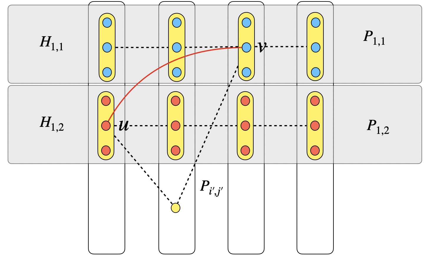
Figure 9: The gray boxes denote the subgraphs $H_{1,1}$ and $H_{1,2}$ that are created w.r.t. paths $P_{1,1}$ and $P_{1,2}$ in the same UPC of $G_{\textsc{dup}}$. If there is an edge between vertices $u$ and $v$ that is added w.r.t. another path $P_{i^{\prime},j^{\prime}}$, it implies that some subpath of $P_{i^{\prime},j^{\prime}}$ connects two vertices in paths $P_{1,1}$ and $P_{1,2}$ together – this is because any edge of $G$ is added “alongside” a path of $G_{\textsc{dup}}$, although it is possible that it shortcuts a couple of layers in between as $H_{i^{\prime},j^{\prime}}$ may have edges between non-consecutive layers. This in turn creates another layered path between $\textnormal{{start}}(P_{1,2})$ and $\textnormal{{final}}(P_{1,1})$, which is not allowed in a UPC, a contradiction.

4.3 A Construction of DUP Graphs

We now present a construction of DUP graphs and prove Proposition 4.5. The construction of these graphs follows a standard approach in the literature, e.g., in [AB16], for creating graphs with many long disjoint shortest paths. For completeness, we provide the construction to incorporate UPCs explicitly (beyond just bounding the number of “critical paths” as in [AB16]) and fine tune the parameters to the range that we need (which is different from the typical range of parameters used in other applications of these graphs that we are aware of).

We first need a basic claim on the existence of a large set of “average-free” vectors.

Claim 4.8.

For any $\ell,d\geqslant 1$, there exists a set $A\subseteq[\ell]^{d}$ with $\left|{A}\right|\geqslant\frac{\ell^{d}}{d\cdot\ell^{2}}$ such that for every multi-set of $t\geqslant 1$ not-all-equal vectors $y_{1},\ldots,y_{t}\in A$, their average $(1/t)\sum_{i=1}^{t}y_{i}$ is not in $A$.

Proof.

Let $A$ be the largest subset of $[\ell]^{d}$ such that all vectors in $A$ have the same $\ell_{2}$-norm. Since the number of different values possible for squared $\ell_{2}$-norm of vectors in $[\ell]^{d}$ is at most $d\cdot\ell^{2}$, we obtain the lower bound in the claim statement on the size of $A$ by the pigeonhole principle.

Let $s$ denote the $\ell_{2}$-norm of the vectors in $A$. Consider any multi-set of $t>1$ not-all-equal vectors $y_{1},\ldots,y_{t}\in A$. We have,

$$\|\frac{1}{t}\sum_{i=1}^{t}y_{i}\|_{2}^{2} =\frac{1}{t^{2}}\left(\sum_{i=1}^{t}\|y_{i}\|^{2}+\sum_{i\neq j}\langle y_{i}\;,\;y_{j}\rangle\right)<\frac{1}{t^{2}}\left(\sum_{i=1}^{t}\|y_{i}\|^{2}+\sum_{i\neq j}\|y_{i}\|\|y_{j}\|\right) y_{i}\neq y_{j} y_{i}$$ (the Cauchy-Schwartz inequality is strict for the pair which exists as ’s are not all equal)

$$=\frac{1}{t^{2}}\left(t\cdot s^{2}+t\cdot(t-1)\cdot s^{2}\right)=s^{2}.$$

The $\ell_{2}$-norm of the average is strictly less than $s$, hence, it cannot be in $A$.       

We now use the existence of the set $A$ in Claim 4.8 to construct our DUP graphs.

A construction of $(p,q,k)$-DUP graphs: $(i)$ Set $d:=\sqrt{\log{\big{(}\frac{n}{k+1}\big{)}}}$ and $\ell:=\left(\frac{n}{(k+1)\cdot(k+2)^{d}}\right)^{1/d}$ and let $A\subseteq[\ell]^{d}$ be the set of vectors in Claim 4.8. $(ii)$ Fix the vertex set $V=V_{1}\cup V_{2}\cup\ldots\cup V_{k+1}$ with $V_{i}:=[(k+2)\cdot\ell]^{d}$ for each $i\in[k+1]$. $(iii)$ For every $x\in[\ell]^{d}$ and $y\in A$, and all $i\in[k]$, add an edge between $$x+i\cdot y\in V_{i}\quad\text{and}\quad x+(i+1)\cdot y\in V_{i+1}.$$

Proof of Proposition 4.5.

The partition of the edge set into $q=\ell^{d}$ UPCs of size $p=\left|{A}\right|\geqslant\ell^{d}/(d\cdot\ell^{2})$ each is as follows. For every $x\in[\ell]^{d}$, we have a UPC $\mathcal{P}_{x}:=\left\{P_{x,y}\mid y\in A\right\}$ of $p$ paths. Each path $P_{x,y}\in\mathcal{P}_{x}$ for $y\in A$ is defined as:

$$P_{x,y}:=(x+y~{},~{}x+2y~{},~{}x+3y~{},~{}\ldots~{},~{}x+(k+1)\cdot y),$$

where edge $(x+i\cdot y,x+(i+1)\cdot y)$ is from the layer $V_{i}$ to layer $V_{i+1}$ for $i\in[k]$. See Figure 10 for an illustration. We now prove that $G$ is indeed a DUP graph with the UPCs $\mathcal{P}_{x}$ for $x\in[\ell]^{d}$.

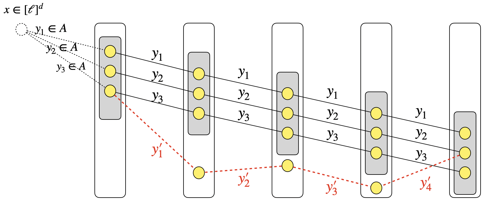
Figure 10: An illustration of the construction of DUP graphs. The circle $x$ at left does not correspond to a vertex and instead is used to define a UPC. The red path cannot exist because it requires $y_{3}+y^{\prime}_{1}+y^{\prime}_{2}+y^{\prime}_{3}+y^{\prime}_{4}=5\cdot y_{2}$ which cannot happen because $A$ is average free.

Firstly, any edge of the graph $G$ is between some $x+i\cdot y$ and $x+(i+1)\cdot y$ for $x\in[\ell]^{d}$ and $y\in A$ and $i\in[k]$. This edge thus belongs to the path $P_{x,y}$ in the UPC $\mathcal{P}_{x}$. Hence, the edges of the graph are partitioned between the UPCs.

Secondly, by the definition, each $P_{x,y}$ is a layered path. Furthermore, the paths in $\mathcal{P}_{x}$ are vertex-disjoint since, for any pair of paths $P_{x,y}$ and $P_{x,y^{\prime}}$ for some $y,y^{\prime}\in A$, their respective vertices in layer $i$, given by $x+i\cdot y$ and $x+i\cdot y^{\prime}$, are only the same if $y=y^{\prime}$.

Finally, consider $z_{s}:=\textnormal{{start}}(P_{x,y})$ and $z_{f}:=\textnormal{{final}}(P_{x,y^{\prime}})$ for some $y,y^{\prime}\in A$; we prove that $z_{s}$ has no layered path to $z_{f}$ in $G$ unless $y=y^{\prime}$, in which case there is only one layered path $P_{x,y}$ (in the entire graph $G$), between $z_{s}$ and $z_{f}$.

By definition, we have

$$z_{s}=x+y\qquad\text{and}\qquad z_{f}=x+(k+1)\cdot y^{\prime}.$$

Suppose there exists a layered path between $z_{s}$ and $z_{f}$. As each edge of the graph connects its both endpoints via a vector in $A$, this means that there exist vectors $y_{1},\ldots,y_{k}\in A$ such that $z_{f}-z_{s}=\sum_{i=1}^{k}y_{i}$. This implies that

$$x+(k+1)\cdot y^{\prime}=z_{f}=z_{s}+\sum_{i=1}^{k}y_{i}=x+y+\sum_{i=1}^{k}y_{i},$$

which in turn means

$$y^{\prime}=\frac{1}{k+1}\cdot\left(y+\sum_{i=1}^{k}y_{i}\right).$$

By Claim 4.8, since $y^{\prime}\in A$, the only possibility is that $(y,y_{1},\ldots,y_{k})$ are all-equal, which means that they are also all equal to $y^{\prime}$. Thus, the only possible layered path between $z_{s}$ and $z_{t}$ is if they belong to the same path $P_{x,y}\in\mathcal{P}_{x}$.

To finalize the proof, we can work out the parameters as follows. The number of vertices is

$$(k+1)\cdot\left((k+2)\cdot\ell\right)^{d}=(k+1)\cdot\left((k+2)\cdot\left(\frac{n}{(k+1)\cdot(k+2)^{d}}\right)^{1/d}\right)^{d}=n,$$

as it should be, hence the choice of $\ell$ and $d$ are consistent with $n$. Moreover, by the upper bound on $k$ and the choice of $d$, we have,

$$q =\ell^{d}=\left(\left(\frac{n}{(k+1)\cdot(k+2)^{d}}\right)^{1/d}\right)^{d}\geqslant\frac{n}{(k+2)^{d+1}}\geqslant\frac{n}{2^{\Theta(1)\cdot(\log{n})^{1/4}\cdot(\log{n})^{1/2}}}\geqslant\frac{n}{2^{\Theta((\log{n})^{3/4})}};$$

$$p \geqslant\frac{\ell^{d}}{\ell^{2}\cdot d}=\frac{q}{\ell^{2}\cdot d}\geqslant\frac{q}{n^{2/d}\cdot\sqrt{\log{n}}}=\frac{q}{2^{2\log n/\sqrt{\log{n/k}}}\cdot\sqrt{\log{n}}}\geqslant\frac{q}{2^{\Theta(\sqrt{\log{n}})}}\geqslant\frac{n}{2^{\Theta((\log{n})^{3/4})}},$$

as desired. This concludes the proof for all graph sizes determined this way from $k$ and $\ell$ by picking $\eta_{p}$ and $\eta_{q}$ to match the hidden constants in the $\Theta$-notation above.

To conclude the proof, we need the construction to work for all large enough integers $n$ as in the statement of the proposition. However, this can be fixed easily using a padding argument, which we postpone to Appendix B.       

5 A Round vs Communication Tradeoff for MIS

We now switch to proving a multi-party communication lower bound for MIS, defined formally as:

Definition 5.1.

For any integers $n,t\geqslant 1$, we define $\textnormal{{MIS}}_{n,t}$ as the communication game of outputting any MIS of a given $n$-vertex graph whose edges are partitioned between $t$ players.

We prove an almost optimal round vs communication tradeoff for MIS in the model of Section 3.1, formalizing 2 from Section 1.

Theorem 1.

For any $r\geqslant 1$ and sufficiently large $n\in\mathbb{N}$, any $r$-round $(r+1)$-party protocol $\pi$ for $\textnormal{{MIS}}_{n,r+1}$ with any constant probability of success strictly more than zero has communication cost

$$\textsc{CC}(\pi)=\Omega\Big{(}\frac{1}{2^{\Theta(r\log^{5/6}(n))}}\cdot n^{1+1/(2^{r}-1)}\Big{)}.$$

The lower bound for semi-streaming algorithms in 1, restated below, now follows.

Corollary 2.

For any integer $p\geqslant 1$ and sufficiently large $n\in\mathbb{N}$, any $p$-pass streaming algorithm for finding any maximal independent set with any constant probability of success strictly more than zero has space

$$\Omega\Big{(}\frac{1}{2^{\Theta(p\log^{5/6}(n))}}\cdot n^{1+1/(2^{p}-1)}\Big{)}.$$

In particular, semi-streaming algorithms require $\Omega(\log\log{n})$ passes.

Proof.

Follows from Theorem 1 and Proposition 3.2 since the number of players and rounds are $O(\log\log{n})$ each, and hence, the space lower bound is at most smaller than the communication one by an $O((\log\log{n})^{2})$ factor; this is subsumed by the $2^{\Theta(\log^{5/6})}$ term of the lower bound.       

We define our hard input distribution in the proof of Theorem 1 in this section, and list its main properties. We then use this distribution in the next section to conclude the proof of Theorem 1.

5.1 A Family of Hard Distributions for MIS

The distributions are defined recursively as a family $\left\{\mathcal{G}_{r}(n)\right\}_{r\geqslant 0}$ where $\mathcal{G}_{r}(n)$ is a hard distribution for $r$-round $(r+1)$-party protocols on $n$-vertex graphs. To avoid ambiguity with the notation for paths, we use ${Q}_{1},{Q}_{2},\ldots,{Q}_{r+1}$ to denote the players in $\mathcal{G}_{r}(n)$. In addition, the input to player ${Q}_{a}$ for $a\in[r+1]$ is denoted by $G_{a}$.

Base case for $r=0$.

The base case is defined vacuously for $r=0$ and $0$-round “protocols” that are supposed to solve a simple yet non-trivial MIS problem (and are hence trivially impossible).

The distribution $\mathcal{G}_{0}(n)$ for $0$-round protocols on $n$-vertex graphs for $n\geqslant 2$. 1. Let $G=(V,E)$ be a graph on $p_{0}=n/2$ vertices $V=\left\{u_{i},v_{i}\mid i\in[p_{0}]\right\}$. 2. For each $i\in[p_{0}]$, the edge $(u_{i},v_{i})$ is independently included in $E$ with probability $1/2$ (independent of the inclusion of the other potential edges $(u_{j},v_{j})$, for $j\neq i$). 3. Player ${Q}_{1}$ receives $G(1):=G$ as the input (this is the only player when $r=0$).

The answer to MIS on $\mathcal{G}_{0}$ contains either one of the vertices $u_{i}$ or $v_{i}$ (but not both) with probability half, and otherwise contains both $u_{i}$ and $v_{i}$ with the remaining probability for each $i\in[p_{0}]$ independently. Thus, a $0$-round “protocol”, namely, one that has to commit to a fixed answer always without checking the input, can only succeed with probability $1/2^{p_{0}}$ on $\mathcal{G}_{0}$.

Distributions for $r\geqslant 1$.

A graph generated by $\mathcal{G}_{r}(n)$ will be an $(n,2^{r+1})$-layered graph created by embedding many $n_{r-1}$-vertex hard instances for $(r-1)$ rounds into $(p_{r},q_{r},2^{r}-1)$-DUP graphs with $b_{r}$ vertices in each layer. We will determine the values of the parameters $p_{r},q_{r},b_{r}$ and $n_{r-1}$ based on $n$ shortly, after defining the distribution itself. Throughout, if clear from the context or not relevant, we may omit the subscripts on $p_{r},q_{r}$, and $b_{r}$, as well as $n$ from $\mathcal{G}_{r}(n)$.

Distribution $\mathcal{G}_{r}(n)$ for $r$-round protocols for $r\geqslant 1$. 1. Pick a fixed $(p_{r},q_{r},2^{r}-1)$-DUP graph $G_{\textsc{dup}}:=(W=W_{1}\cup\ldots\cup W_{2^{r}},E_{\textsc{dup}})$ with $b_{r}$ vertices in each layer and thus $b_{r}\cdot 2^{r}$ vertices in total. 2. Sample $p_{r}\cdot q_{r}$ independent instances $\mathcal{H}:=\left\{H_{i,j}\mid i\in[q_{r}],j\in[p_{r}]\right\}$ from $\mathcal{G}_{r-1}(n_{r-1})$. 3. Create two identical copies of the graph $\widetilde{G}_{L}=\widetilde{G}_{R}:=\textnormal{{embed}}(\mathcal{H}\rightarrow G_{\textsc{dup}})$. 4. For $a\in[r]$, player ${Q}_{a}$ receives the edges in both $\widetilde{G}_{L}$ and $\widetilde{G}_{R}$ that correspond to $H_{i,j,a}$ for $i\in[q_{r}],j\in[p_{r}]$ where $H_{i,j,a}$ is the subgraph of $H_{i,j}$ given to the $a^{\text{th}}$ player in $\mathcal{G}_{r-1}(n_{r-1})$. 5. Pick $t$ uniformly at random from $[q_{r}]$ and let $\mathcal{P}^{\star}:=\mathcal{P}_{t}$ be the $t$-th UPC in $G_{\textsc{dup}}$, referred to as the special UPC. Let $W^{\star}\subseteq W$ be the set of vertices in $G_{\textsc{dup}}$ incident to $\mathcal{P}^{\star}$. 6. Player ${Q}_{r+1}$ receives a bipartite clique between $\left\{(u,*)\mid u\in W\setminus W^{\star}\right\}$ in $\widetilde{G}_{L}$ and $\widetilde{G}_{R}$.

Figure 11 gives an illustration of our hard distribution.

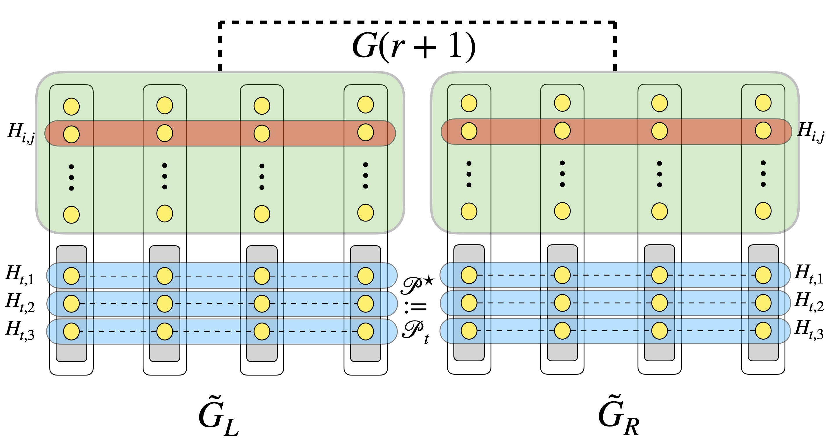
Figure 11: An illustration of the distribution $\mathcal{G}_{r}(n)$. The paths at the bottom correspond to the UPC $\mathcal{P}^{\star}$; each path is “replaced” with an instance $H$ from $\mathcal{G}_{r-1}(n_{r-1})$ via the embedding product. Since the embedding product affects the entire graph, the paths in other UPCs are also replaced by instances from $\mathcal{G}_{r-1}(n_{r-1})$, e.g., for the top (red) block (remaining instances are not drawn). The last player ${Q}_{r+1}$ receives a bipartite clique between the vertices corresponding to $W\setminus W^{\star}$ in $\widetilde{G}_{L}$ and $\widetilde{G}_{R}$, denoted by the top (green) blocks. Other players ${Q}_{a}$ for $a\in[r]$ receive the inputs of the $a^{\text{th}}$ player in all instances $H$ sampled from $\mathcal{G}_{r-1}(n_{r-1})$ when placed inside graphs $\widetilde{G}_{L}$ and $\widetilde{G}_{R}$.

Definitions and Notation for Distribution $\mathcal{G}_{r}(n)$

We set up the following notation for the distribution $\mathcal{G}_{r}(n)$ for $r\geqslant 1$. For any $a\in[r+1]$, let $\mathcal{G}_{r,a}(n)$ denote the distribution of edges in the input graph that are given to player ${Q}_{a}$. Thus, the distribution $\mathcal{G}_{r}(n)$ is a joint distribution of $(\mathcal{G}_{r,1}(n),\ldots,\mathcal{G}_{r,r+1}(n))$.

An instance of the $\textnormal{{MIS}}_{n,r+1}$ sampled from $\mathcal{G}_{r}(n)$ is a graph $G$ with $n$ vertices together with its edge partitioning between the $r+1$ players. With a slight abuse of notation, we sometimes refer to $G$ sampled from $\mathcal{G}_{r}(n)$, i.e., $G\sim\mathcal{G}_{r}(n)$, as the entire instance, where the edge partitioning between the players is implicit. Any $G\sim\mathcal{G}_{r}(n)$ contains $q_{r}\cdot p_{r}$ instances $H_{1,1},\ldots,H_{q_{r},p_{r}}$ sampled from $\mathcal{G}_{r-1}(n_{r-1})$ that are embedded as part of both $\widetilde{G}_{L}$ and $\widetilde{G}_{R}$. We refer to these $(r-1)$-round instances as the sub-instances of $G$. For any $i\in[q_{r}],j\in[p_{r}]$, we further write $\widetilde{E}_{L,i,j}$ and $\widetilde{E}_{R,i,j}$ to denote the edges inserted to, respectively, $\widetilde{G}_{L}$ and $\widetilde{G}_{R}$ as part of the embedding of $H_{i,j}$ into $G_{\textsc{dup}}$.

Among the sub-instances of any $G\sim\mathcal{G}_{r}(n)$, there are $p_{r}$ sub-instances that correspond to the paths in the special UPC $\mathcal{P}^{\star}$; we denote them by $\mathcal{H}^{\star}$ and call them the special sub-instances of $G$. We enumerate these special sub-instances by $H_{t,j}$ for $t\in[q_{r}]$ being the index of the special UPC $\mathcal{P}^{\star}=\mathcal{P}_{t}$ and $j$ ranging over $[p_{r}]$.

For any $j\in[p_{r}]$, define the special subgraphs $G^{\star}_{L,j}$ and $G^{\star}_{R,j}$ as the subgraphs of $\widetilde{G}_{L}$ and $\widetilde{G}_{R}$ on edges of special sub-instance $H_{t,j}$, i.e., with edges $\widetilde{E}_{L,t,j}$ and $\widetilde{E}_{R,t,j}$, respectively.

The Choice of Parameters and Their Ranges

We now specify how the parameters $p_{r},q_{r},b_{r}$, and $n_{r-1}$ are chosen, the restriction we have on their ranges, and their “validity” in their recursive calls (and Proposition 4.5).

Parameters $b_{r},n_{r-1}$.

Let $n_{0}$ be an arbitrarily large constant to be determined later (this controls the probability of success of the protocols). The distribution $\mathcal{G}_{r}(n)$ for $r\geqslant 0$ rounds requires that

$$n\geqslant\frac{1}{2}\cdot(2n_{0})^{{2}^{r}-1}.$$ (3)

For $r=1$, $n_{0}$ is already defined and $b_{1}$ is defined from $n$ as

$$b_{1}=\left(\frac{n}{2\cdot n_{0}}\right).$$ (4)

For $r>1$, $b_{r}$ and $n_{r-1}$ are defined from $n$ via the following equations (recall that $(a)\uparrow(b)=a^{b}$)

$$\begin{split}&b_{r}=\left(n_{r-1}\right)\uparrow\left(1+\frac{1}{2^{r-1}-1}\right),\\ &2\cdot b_{r}\cdot n_{r-1}=n,\end{split}$$ (5)

which implies that

$$\begin{split}n_{r-1}&=\left(\frac{n}{2}\right)\uparrow\left(\frac{2^{r-1}-1}{2^{r}-1}\right)\\ b_{r}&=\left(\frac{n}{2}\right)\uparrow\left(\frac{2^{r-1}}{2^{r}-1}\right).\end{split}$$ (6)

In the distribution $\mathcal{G}_{r}(n)$ for any $r\geqslant 1$, we call the distribution $\mathcal{G}_{r-1}(n_{r-1})$. For $r=1$, $\mathcal{G}_{1}(n)$ calls $\mathcal{G}_{0}(n_{0})$ which satisfies Eq 3 as

$$\frac{1}{2}\cdot(2n_{0})^{2^{1}-1}=n_{0}.$$

For $r>1$, $\mathcal{G}_{r}(n)$ calls $\mathcal{G}_{r-1}(n_{r-1})$ and by the choice of $n_{r-1}$ in Eq 6, we have,

$$n_{r-1}=\left(\frac{n}{2}\right)\uparrow\left(\frac{2^{r-1}-1}{2^{r}-1}\right)\underset{\textnormal{\lx@cref{creftypecap~refnum}{eq:n-r-relation}}}{\geqslant}\left(\frac{1}{2}\cdot(2n_{0})^{{2}^{r}-1}\right)\uparrow\left(\frac{2^{r-1}-1}{2^{r}-1}\right)\geqslant\frac{1}{2}\cdot\left(2n_{0}\right)^{2^{r-1}-1},$$ (7)

which means the call to $\mathcal{G}_{r-1}(n_{r-1})$ also satisfies Eq 3 for $r-1$. This gives us the following.

Observation 5.2.

For any $r\geqslant 1$, if the distribution $\mathcal{G}_{r}(n)$ satisfies Eq 3 for $n$, then any distribution $\mathcal{G}_{r^{\prime}}(n^{\prime})$ for $r^{\prime}<r$ called recursively in $\mathcal{G}_{r}$ also satisfies Eq 3 for $r^{\prime},n^{\prime}$.

Parameters $p_{r},q_{r}$ for $r\geqslant 1$.

Recall that we use a $(p_{r},q_{r},2^{r}-1)$-DUP graph with $b_{r}$ vertices in each layer in $\mathcal{G}_{r}$. This means the the total number of vertices in this DUP graph is $b_{r}\cdot 2^{r}$. We define the parameters $p_{r}$ and $q_{r}$ as follows:

$$\begin{split}p_{r}&:=\frac{b_{r}\cdot 2^{r}}{\exp(\eta_{p}\cdot(\ln(b_{r}\cdot 2^{r}))^{3/4})},\\ q_{r}&:=\frac{b_{r}\cdot 2^{r}}{\exp(\eta_{q}\cdot(\ln(b_{r}\cdot 2^{r}))^{3/4})}.\end{split}$$ (8)

Firstly, these bounds match those of Proposition 4.5 and thus we can apply the proposition to prove the existence of the required DUP graphs in our distribution. We should also verify that

$$2^{r}-1\leqslant 2^{(\log{(b_{r}\cdot 2^{r})})^{1/4}},$$

which is required by Proposition 4.5. For $r=1$, the LHS is $1$ and this holds trivially. For $r>1$, we have by Eq 6 that

$$b_{r}=\left(\frac{n}{2}\right)\uparrow\left(\frac{2^{r-1}}{2^{r}-1}\right)\underset{\textnormal{\lx@cref{creftypecap~refnum}{eq:n-r-relation}}}{\geqslant}\left(\frac{1}{2}\cdot(2n_{0})^{{2}^{r}-1}\right)\uparrow\left(\frac{2^{r-1}}{2^{r}-1}\right)\geqslant\frac{1}{2}\cdot\left((2n_{0})^{{2}^{r-1}}\right).$$

This satisfies the above equation because

$$\log{(2^{r}-1)}\leqslant r\qquad\text{whereas}\qquad(\log{(b_{r}\cdot 2^{r})})^{1/4}\geqslant 2^{r-4}\cdot\log{(n_{0})}$$

and thus we obtain the equation for any large constant $n_{0}$ (with quite some room to spare).

Observation 5.3.

For any $r\geqslant 1$, if the distribution $\mathcal{G}_{r}(n)$ satisfies Eq 3 for $n$, then the DUP graphs created in $\mathcal{G}_{r}$ (and in any recursive call to $\mathcal{G}_{r^{\prime}}$ for $r^{\prime}<r$) with the given parameters $p_{r}$ and $q_{r}$ do exist (by Proposition 4.5).

5.2 Basic Properties of the Distributions $\left\{\mathcal{G}_{r}(n)\right\}_{r\geqslant 1}$

We establish some basic properties of the distribution $\mathcal{G}_{r}(n)$ for $r\geqslant 1$ in this subsection. We then use these to define search predicates that reduce our task of proving the lower bound for MIS to determining the ability of protocols in figuring out a certain predicate for graphs sampled from $\mathcal{G}_{r}$.

The first property identifies the “real input” to the players.

Property 1.

For any $a\in[r]$, the input of player ${Q}_{a}$ in $G_{a}\sim\mathcal{G}_{r,a}(n)$ is determined deterministically by the input of the $a^{\text{th}}$ player in all sub-instances in $\mathcal{H}$, i.e., $\mathcal{H}_{a}:=\left\{H_{i,j,a}\mid i\in[q_{r}],j\in[p_{r}]\right\}$. The input of player ${Q}_{r+1}$ is deterministically determined by the index $t\in[q_{r}]$ of the special UPC.

Proof.

The choice of $G_{\textsc{dup}}$ is fixed in $\mathcal{G}_{r}(n)$ and does not include any randomness (think of it as being “hardcoded” in the definition of the distribution). For any $a\in[r]$, given only $\mathcal{H}_{a}$, player ${Q}_{a}$ can know the edges of $\widetilde{G}_{L}$ and $\widetilde{G}_{R}$ that belong to its input. Similarly, given only $t$, player ${Q}_{r+1}$ can know what vertices of $\widetilde{G}_{L}$ and $\widetilde{G}_{R}$ are in $W^{\star}$ and thus which edges should be added to the bipartite clique between vertices corresponding to $W\setminus W^{\star}$ in $\widetilde{G}_{L}$ and $\widetilde{G}_{R}$.       

The next property shows that the distributions $\left\{\mathcal{G}_{r}(n)\right\}_{r\geqslant 0}$ are product distributions – a fact which is used crucially in our lower bound arguments.

Property 2.

For any $r\geqslant 0$, the distribution $\mathcal{G}_{r}(n)$ is a product distribution, i.e.,

$$\mathcal{G}_{r}(n)=\mathcal{G}_{r,1}(n)\times\mathcal{G}_{r,2}(n)\times\cdots\times\mathcal{G}_{r,r+1}(n).$$

Proof.

The proof is by induction on $r$. The base case when $r=0$ is trivial as the entire graph is given to ${Q}_{1}$. Let us assume that the statement is true for $r=\ell$ and we prove it for $r=\ell+1$.

The input to players in $\mathcal{G}_{\ell+1}(n)$, by Property 1 is determined by $q_{\ell+1}\cdot p_{\ell+1}$ sub-instances sampled from $\mathcal{G}_{\ell}(n_{\ell})$ (for players ${Q}_{1}$ to ${Q}_{\ell+1}$) and by $t\in[q_{\ell+1}]$ (for player ${Q}_{\ell+2}$). The distribution of each sub-instance $H_{i,j}$ for $i\in[q_{\ell+1}]$ and $j\in[p_{\ell+1}]$ is a product distribution of the inputs to ${Q}_{a}$ for all $a\in[\ell+1]$ by the induction hypothesis. These sub-instances are also all sampled independently of each other, thus making the collective input to players ${Q}_{1}$ to ${Q}_{\ell+1}$ independent of each other. Finally, the index $t\in[q_{\ell+1}]$ is sampled independent of all other variables, implying the input to player ${Q}_{\ell+2}$ is also independent of the rest, completing the proof.       

The next two properties together identify the key properties of special subgraphs and their role w.r.t. any MIS of the input graph.

Property 3.

The special subgraphs are all vertex-disjoint. Moreover, the induced subgraph of $\widetilde{G}_{L}$ (resp. $\widetilde{G}_{R}$) on the vertices corresponding to the special subgraphs contains only the edges of these subgraphs, i.e., the edges of $G^{\star}_{L,j}$ (resp. $G^{\star}_{R,j}$) for all $j\in[p_{r}]$.

Proof.

The special subgraphs inserted to either $\widetilde{G}_{L}$ or $\widetilde{G}_{R}$ are part of the embedding product of $\textnormal{{embed}}{(\mathcal{H}\rightarrow G_{\textsc{dup}})}$ corresponding to the special UPC $\mathcal{P}^{\star}$. Thus, by Lemma 4.7, we know that they are vertex-disjoint and no other edges from any other subgraphs are present in the vertices of the special subgraphs.       

Property 4.

For any graph $G\sim\mathcal{G}_{r}(n)$ for $r\geqslant 1$, any MIS $S$ of $G$ also contains an MIS for every special subgraph $G^{\star}_{L,1},\ldots,G^{\star}_{L,p_{r}}$ or every special subgraph $G^{\star}_{R,1},\ldots,G^{\star}_{R,p_{r}}$.

Proof.

We consider three possible cases for the proof.

Case 1.

Suppose first that there exists a vertex $v\in S$ which (1) belongs to $\widetilde{G}_{L}$ and (2) corresponds to some vertex in $W\setminus W^{\star}$. Figure 12 gives an illustration of this case.

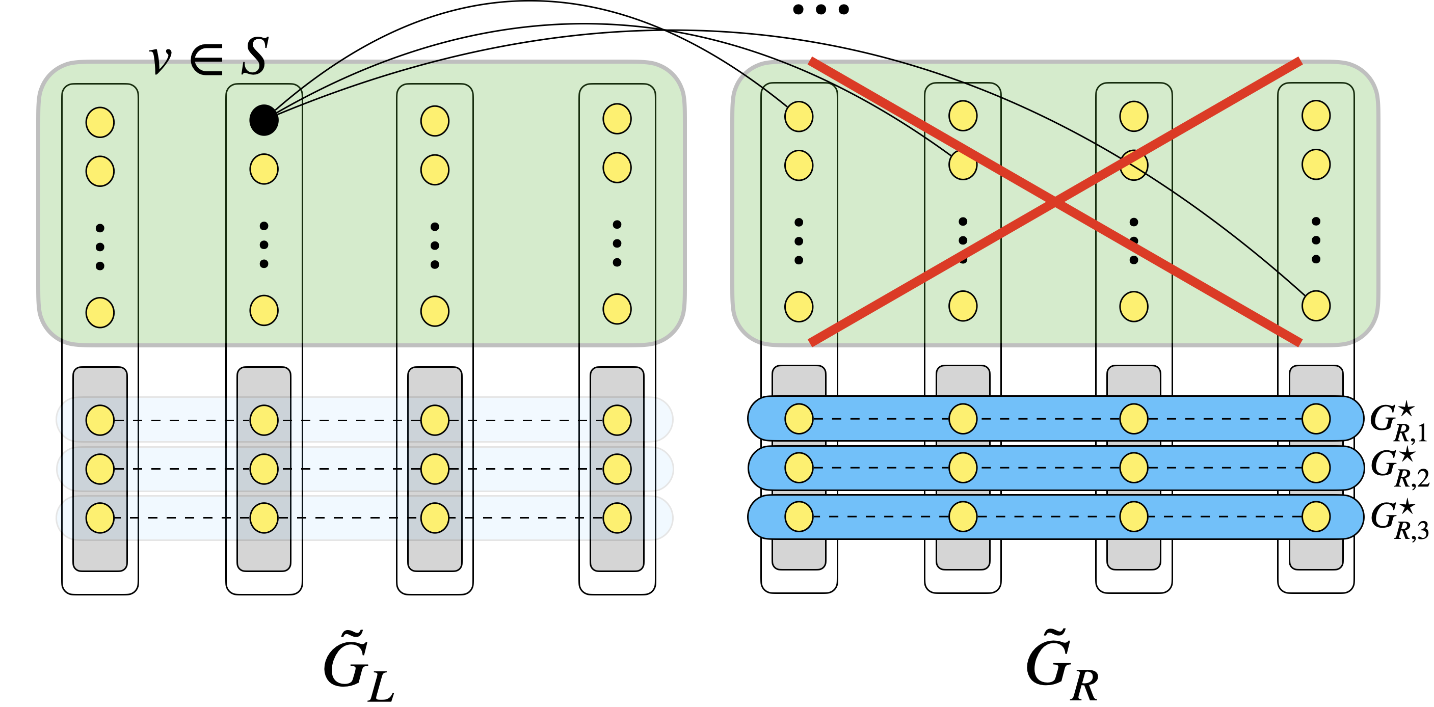
Figure 12: An illustration of case $1$: picking vertex $v$ in the MIS “removes” all vertices on $\widetilde{G}_{L}$ that are not part of the special subgraphs as the remaining ones are all neighbor to $v$ (not all edges of $v$ are drawn). Since the special subgraphs are now isolated, the MIS of $G$ now needs to contain a separate MIS for each of the special subgraphs in $\widetilde{G}_{R}$ in bottom right (drawn in blue).

Since $G_{r+1}\subseteq G$ is a bipartite clique between vertices corresponding to $W\setminus W^{\star}$ in $\widetilde{G}_{L}$ and $\widetilde{G}_{R}$, we have that all vertices corresponding to $W\setminus W^{\star}$ in $\widetilde{G}_{R}$ are now incident on $v$ and cannot be part of the MIS $S$. The remaining vertices in $\widetilde{G}_{R}$ are incident on $W^{\star}$ and thus $S$ also needs to contain an MIS of the induced subgraph of $\widetilde{G}_{R}$ on vertices corresponding to $W^{\star}$ or equivalently $\mathcal{P}^{\star}$ – this is because these vertices do not have any edge to $\widetilde{G}_{L}$ and also no vertex of $\widetilde{G}_{R}$ outside these can be part of $S$.

We can now apply the main property of the embedding product, i.e., Lemma 4.7, captured in Property 3 to have that the induced subgraph of $\widetilde{G}_{R}$ on the vertices corresponding to the UPC $\mathcal{P}^{\star}$ is a vertex-disjoint union of subgraphs $G^{\star}_{R,1},\ldots,G^{\star}_{R,p_{r}}$. This immediately implies that the MIS of this subgraph of $\widetilde{G}_{R}$ should be a union of the MISes of $G^{\star}_{R,1},\ldots,G^{\star}_{R,p_{r}}$, which means the MIS $S$ contains an MIS for each of these special subgraphs.

Case 2.

Suppose the symmetric case that there exists a vertex $v\in S$ which (1) belongs to $\widetilde{G}_{R}$ and (2) corresponds to some vertex in $W\setminus W^{\star}$. The same exact argument implies that now $S$ should contain an MIS for every special subgraph $G^{\star}_{L,1},\ldots,G^{\star}_{L,p_{r}}$ instead.

Case 3.

Finally, suppose that no vertex in $S$ corresponds to a vertex of $W\setminus W^{\star}$ in either of $\widetilde{G}_{L}$ or $\widetilde{G}_{R}$. This, similar to the above, implies that $S$ should contain an MIS for the induced subgraph of $\widetilde{G}_{L}$ on vertices corresponding to $W^{\star}$ and the induced subgraph of $\widetilde{G}_{R}$ on vertices corresponding to $W^{\star}$. This in turn, again, as above, implies that $S$ now contains an MIS for every special subgraph $G^{\star}_{L,1},\ldots,G^{\star}_{L,p_{r}}$ and every $G^{\star}_{R,1},\ldots,G^{\star}_{R,p_{r}}$.       

5.3 Search Sequences and Predicates

Before getting to analyze the distributions $\left\{\mathcal{G}_{r}(n)\right\}_{r\geqslant 1}$, we need one other set of definitions, which capture the notion of hierarchical embeddings in our lower bounds.

At a high level, the analysis goes as follows. We are hiding the choice of the special UPC of the instance from the first $r$ players in the first round, then UPC of special sub-instances from the first $r-1$ players in the second round, and so on and so forth, until at the end of the last round; at that point, we reach the “inner most” graphs sampled from $\mathcal{G}_{0}$, whose edges are still hidden from the players, and now there is no more round to compute the answer. Making this intuition precise is going take work, but hopefully this provides some intuition for the following definitions.

Notation.

Fix any $r\geqslant 1$. We use $p_{j},q_{j},n_{j}$ for $0\leqslant j<r$ to denote the parameters $p,q,n$ in the instances sampled from the hard distribution for $j$ rounds, i.e., $\mathcal{G}_{j}$, in the construction of the hard distribution on $r$ rounds with $n$ vertices, i.e., $\mathcal{G}_{r}(n)$.

Definition 5.4.

For $r\geqslant 0$, we define $K=(k_{r},k_{r-1},\ldots,k_{1})$ to be a valid search sequence if $k_{i}\in[p_{i}]$ for each $i\in[r]$ ($K=\emptyset$ is the only valid search sequence for $r=0$). We interpret a search sequence on a graph $G=G_{r}\sim\mathcal{G}_{r}(n)$ as: • $k_{r}$ points to the $k_{r}^{\textnormal{th}}$ special sub-instance of $G_{r}$, namely, $G_{r-1}:=H_{t_{r},k_{r}}\sim\mathcal{G}_{r-1}$ where $t_{r}$ is the index of the special UPC of $G_{r}$; • $k_{r-1}$ points to the $k_{r-1}^{\textnormal{th}}$ special sub-instance of $G_{r-1}$, namely, $G_{r-2}:=H_{t_{r-1},k_{r-1}}\sim\mathcal{G}_{r-2}$ where $t_{r-1}$ is the index of the special UPC of $G_{r-1}$; • We continue like this until $k_{1}$ points to the $k_{1}^{\textnormal{th}}$ special sub-instance of $G_{1}$, namely, $G_{0}:=H_{t_{1},k_{1}}\sim\mathcal{G}_{0}$ where $t_{1}$ is the index of the special UPC of $G_{1}$. • We now have a unique instance $G_{0}$ of $\mathcal{G}_{0}$ defined by $K$. Finally, we define the search predicate of a $G\sim\mathcal{G}_{r}(n)$ and a search sequence $K$ as: $$\mathbb{P}_{r}(G,K):=\textnormal{a string in $\left\{0,1\right\}^{p_{0}}$ where the $i$-th bit is $1$ iff $(u_{i},v_{i})$ is an edge in $G_{0}$.}$$

Figure 13 gives an illustration of this definition.

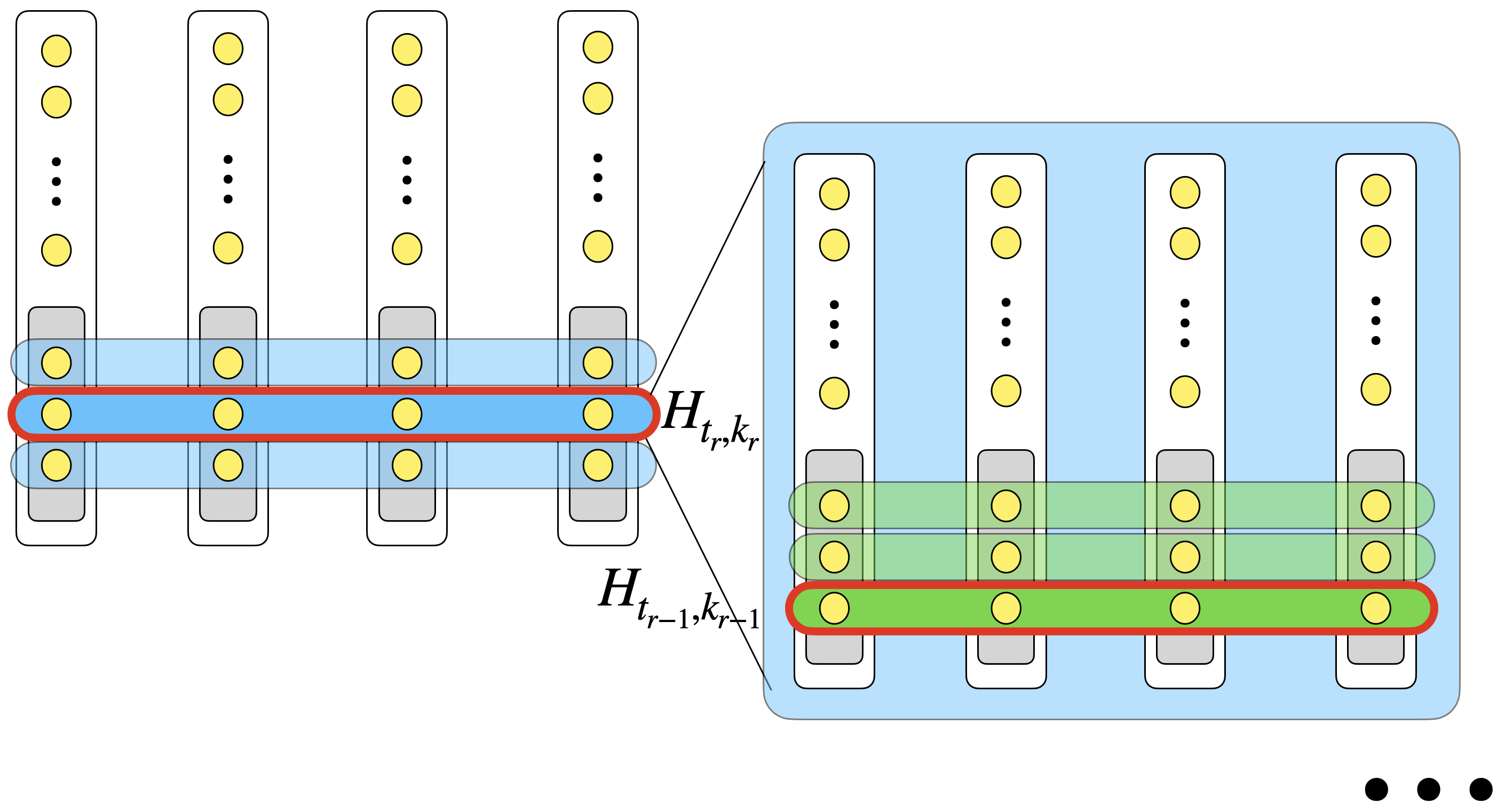
Figure 13: An illustration of a search sequence. Here, $k_{r}$ picks a special sub-instance $H_{t_{r},k_{r}}$ from $\mathcal{G}_{r-1}$ (with $t_{r}$ being the index of the special UPC of the outer instance), and then “inside” that instance, $k_{r-1}$ picks another sub-instance $H_{t_{r-1},k_{r-1}}$ from $\mathcal{G}_{r-2}$ (with $t_{r-1}$ being the index of the special UPC of the instance $H_{t_{r},k_{r}}$), and this continues on.

Let $\pi$ be any $(r+1)$-party communication protocol on inputs sampled from $\mathcal{G}_{r}(n)$, and let $\Pi=\Pi(G)$ be the transcript of $\pi$ at the end of $r$ rounds on an input $G\sim\mathcal{G}_{r}(n)$. We say that the protocol $\pi$ solves the search predicate $\mathbb{P}_{r}$ for input graph $G$, if only given the transcript $\Pi$ and any search sequence $K$ (with no further access to $G$), $\mathbb{P}_{r}(G,K)$ can be deterministically determined for all valid search sequences $K$. We shall emphasize that the search sequence $K$ is not a part of the input to the protocol $\pi$ (and is in fact even independent of the input graph $G$).

The following lemma shows why search sequences are important to us.

Lemma 5.5.

For every $\delta\in(0,1)$, any $(r+1)$-party protocol $\pi$ that outputs an MIS of $G\sim\mathcal{G}_{r}(n)$ with probability at least $\delta$, also solves the search predicate $\mathbb{P}_{r}(G,K)$ for every valid search sequence $K$ with probability at least $\delta$.

Proof.

We claim that:

For any $r\geqslant 0$, any MIS of $G\sim\mathcal{G}_{r}(n)$ uniquely determines $\mathbb{P}_{r}(G,K)$ for all valid search sequences $K$.

We can then conclude the proof as follows. Protocol $\pi$ will be computing some MIS of $G$ with probability at least $\delta$. Thus, whenever $\pi$ succeeds, the transcript $\Pi$ contains an MIS that can be used to solve the predicate $\mathbb{P}_{r}(G,K)$ for all $K$ with probability at least $\delta$ as well.

We now prove the above statement by induction on $r$. The base case when $r=0$ is a graph $G_{0}$ consisting of $n_{0}=2p_{0}$ vertices $u_{i}$ and $v_{i}$ for each $i\in[p_{0}]$ and $K=\emptyset$. Each such $u_{i}$ and $v_{i}$ pair for $i\in[p_{0}]$ is possibly an edge in $G_{0}$. If the edge does exist, any MIS necessarily should have exactly one of $u_{i}$ or $v_{i}$ but not both, whereas if the edge does not exist, then any MIS of $G_{0}$ should contain both $u_{i}$ and $v_{i}$. Thus, given any MIS of $G_{0}\sim\mathcal{G}_{0}$, we can determine the predicate $\mathbb{P}_{0}(G,\emptyset)$.

For the induction step, suppose the statement is true for $r-1$ and we prove it for $r$. Let $K:=(k_{r},\ldots,k_{1})$ be any search sequence. By Property 4, any MIS of $G\sim\mathcal{G}_{r}$ also contains an MIS either for every special subgraph $G^{\star}_{L,1},\ldots,G^{\star}_{L,p_{r}}$ or for every special subgraph $G^{\star}_{R,1},\ldots,G^{\star}_{R,p_{r}}$. In particular, it contains an MIS for either $G^{\star}_{L,k_{r}}$ or $G^{\star}_{R,k_{r}}$. Both these graphs are identical and correspond to the $k_{r}^{\textnormal{th}}$ special sub-instance $H_{t,k_{r}}$ in $G$ where $t$ is the index of the special UPC. As $H_{t,k_{r}}\sim\mathcal{G}_{r-1}$, by the induction hypothesis, an MIS of $H_{t,k_{r}}$ uniquely determines

$$\mathbb{P}_{r-1}(H_{t,k_{r}},(k_{r-1},k_{r-2},\ldots,k_{1})).$$

But, by definition, we also have

$$\mathbb{P}_{r}(G,K)=\mathbb{P}_{r-1}(H_{t,k_{r}},(k_{r-1},k_{r-2},\ldots,k_{1})),$$

as $k_{r}\in K$ is just pointing to the special sub-instance $H_{t,k_{r}}$. This finalizes the proof.       

6 Analysis of the Hard Distribution

We present the analysis of the lower bound for distributions $\left\{\mathcal{G}_{r}\right\}_{r\geqslant 1}$ in this section, and conclude the proof of Theorem 1. By Lemma 5.5, we need to focus on the ability of protocols for solving the search predicate. The following lemma captures our lower bound for this task.

Lemma 6.1.

For any $r\geqslant 1$, any $r$-round protocol $\pi$ that given $G\sim\mathcal{G}_{r}(n)$ (for $n,r$ satisfying Eq 3), can solve $\mathbb{P}_{r}$ on input graph $G$ with probability of success at least

$$2^{-p_{0}}\cdot\left(1+\frac{r}{20\cdot(r+1)}\right)$$

has communication cost

$$\textsc{CC}(\pi)\geqslant s_{r}(n):=\frac{1}{{n_{0}}^{2}\cdot(2^{p_{0}}\cdot 40\cdot c_{\textnormal{comp}})^{r}\cdot((r+1)!)^{2}\cdot e^{3r\ln^{5/6}(n)}}\cdot\left({(n)}\uparrow\left(1+\frac{1}{2^{r}-1}\right)\right).$$

We do note that ignoring all extra (and lower order) terms in the lemma (that are needed for a proper inductive argument), the lemma simply says that obtaining any probability of success better than $2^{-p_{0}}$ (an arbitrarily small constant) requires roughly $n^{1+1/(2^{r}-1)}$ communication.

We prove Lemma 6.1 inductively using a round elimination argument: if we have a “very good” $r$-round protocol, then we should be able to eliminate its first round and also obtain a “good enough” $(r-1)$-round protocol; keep doing this then eventually bring us to a “non-trivial” protocol for the $r=0$ case, which we know cannot exist. The following lemma—which is the heart of the proof—allows us to establish the induction step.

Lemma 6.2.

For every $0<\varepsilon<\delta<1$ and integer $s\geqslant 1$, the following is true. Suppose there is a deterministic $r$-round $(r+1)$-party protocol $\pi_{r}$ with communication cost $\textsc{CC}(\pi_{r})\leqslant s$ that solves predicate $\mathbb{P}_{r}$ with probability at least $\delta$ for a graph $G\sim\mathcal{G}_{r}(n)$ (for $n,r$ satisfying Eq 3). Then, for constant $c_{\textnormal{comp}}$ (from Eq 2), there is an $(r-1)$-round $r$-party deterministic protocol $\pi_{r-1}$ with communication cost

$$\textsc{CC}(\pi_{r-1})\leqslant\frac{c_{\textnormal{comp}}}{\varepsilon}\cdot(\frac{s}{p_{r}}+r^{2})$$

that solves $\mathbb{P}_{r-1}$ for $G^{\prime}\sim\mathcal{G}_{r-1}(n_{r-1})$ (for $n_{r-1}$ from Eq 6) with probability of success at least

$$\delta-\varepsilon-\sqrt{\frac{s}{2p_{r}\cdot q_{r}}}.$$

We spend the bulk of this section in proving Lemma 6.2. We then use this lemma to prove Lemma 6.1 easily in Section 6.4 and subsequently use it to conclude the proof of Theorem 1 in Section 6.5.

6.1 The Setup for the Proof of Lemma 6.2

We now start the proof of Lemma 6.2 which is the most technical part of the paper. Fix any $r\geqslant 1$ and let $\pi_{r}$ be a $r$-round $(r+1)$-party protocol for solving $\mathbb{P}_{r}$ with the parameters specified in Lemma 6.2. We further define (or recall) the following notation:

• $\mathcal{G}_{r,a}(n)$ for $a\in[r+1]$ to denote the distribution of the input subgraph $G_{a}$ given to player ${Q}_{a}$; we further use $H_{a}$ to denote the input of ${Q}_{a}$ in a specific sub-instance $H\in\mathcal{H}(G)$.

• ${\mathsf{t}}$ to denote the random variable for the index $t\in[q_{r}]$ of the special UPC picked in $\mathcal{G}_{r}(n)$.

• $H_{i,*}$ for any $i\in[q_{r}]$ to denote the sub-instances $(H_{i,1},H_{i,2},\ldots,H_{i,p_{r}})$ together in $G\sim\mathcal{G}_{r}(n)$. The sub-instances given to player ${Q}_{a}$ for $a\in[r+1]$ are denoted by $H_{i,*,a}=(H_{i,1,a},H_{i,2,a},\ldots,H_{i,p_{r},a})$.

• $\Pi=(\Pi_{1},\ldots,\Pi_{r})$ as the set of messages communicated by the players in rounds $1$ to $r$. Similarly, we use $\Pi_{i,a}$ for $a\in[r+1]$ to denote the messages of player ${Q}_{a}$ in round $i\in[r]$, and $\Pi_{*,a}$ to denote all messages of ${Q}_{a}$. We use ${\mathsf{\Pi}},{\mathsf{\Pi}}_{i},$ and ${\mathsf{\Pi}}_{i,a}$ as the corresponding random variables for these messages.

Our goal is to go from a $r$-round $(r+1)$-party protocol $\pi_{r}$ for $\mathbb{P}_{r}$ with communication cost $s$ and probability of success $\delta$, to a $(r-1)$-round $r$-party protocol $\pi_{r-1}$ for $\mathbb{P}_{r-1}$ with communication cost $\approx s/(\varepsilon\cdot p_{r})$ and success probability $\approx\delta-\varepsilon-\sqrt{s/(p_{r}\cdot q_{r})}$. We do this in two steps:

• Step 1: We first shave off one player from $\pi_{r}$ and obtain an intermediate $r$-party protocol $\pi^{\prime}$ with communication cost $\approx s/(\varepsilon\cdot p_{r})$ and success probability $\approx\delta-\varepsilon$ for $\mathbb{P}_{r-1}$. However, $\pi^{\prime}$ still has $r$ rounds instead of our desired $(r-1)$ rounds.

• Step 2: We then shave off one round from $\pi^{\prime}$ and obtain the protocol $\pi_{r-1}$ without increasing the communication but by decreasing the success probability with another $\approx\sqrt{s/(p_{r}\cdot q_{r})}$ term.

We implement each step in the following two subsections. We do emphasize that these steps are not entirely blackbox and this partitioning into the two steps is more for the simplicity of exposition (and there will be some intermediate steps as well). Figure 14 gives a schematic organization of these steps, in particular, the protocols we build along the way and their properties.

​​​​​​

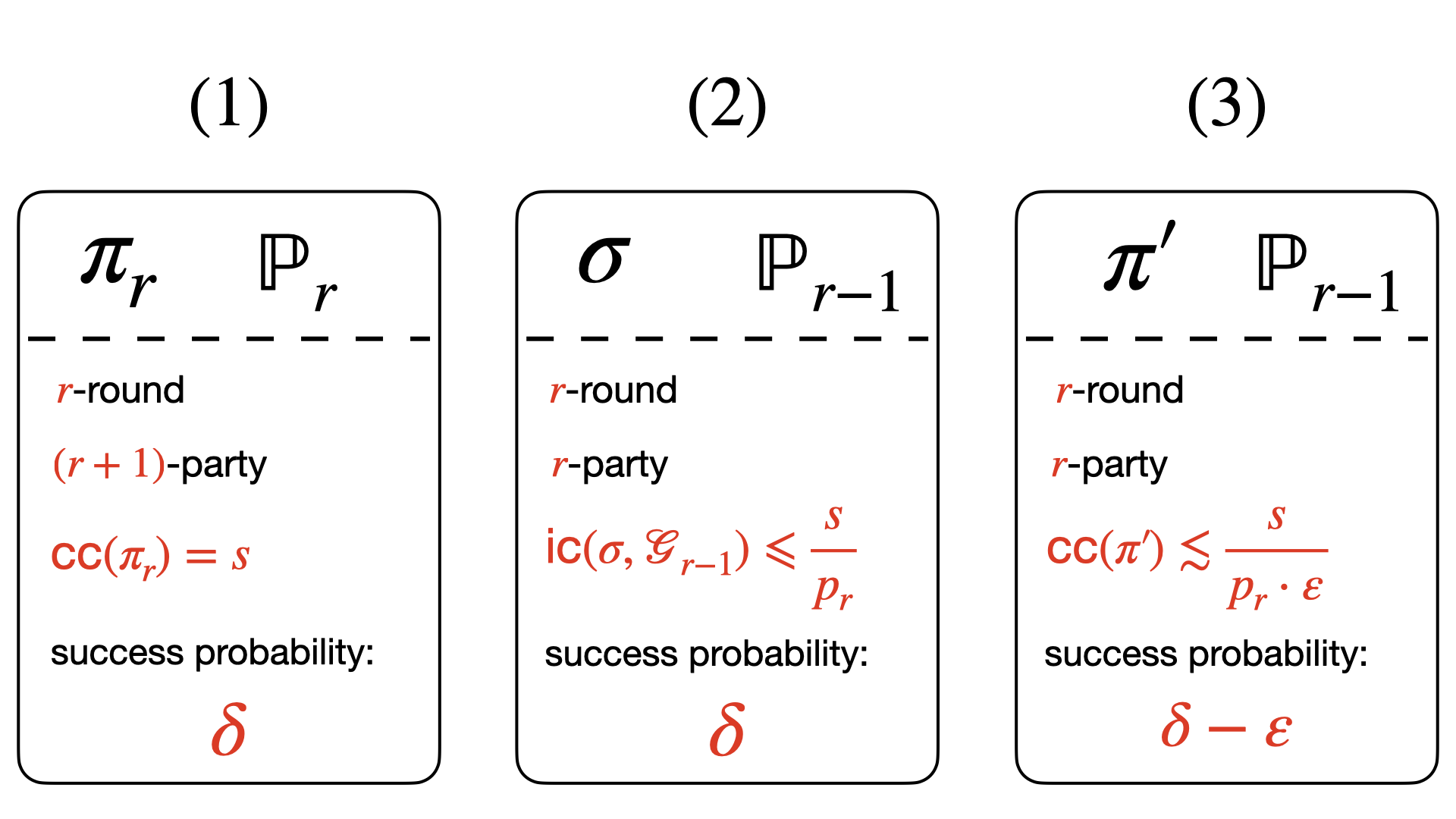
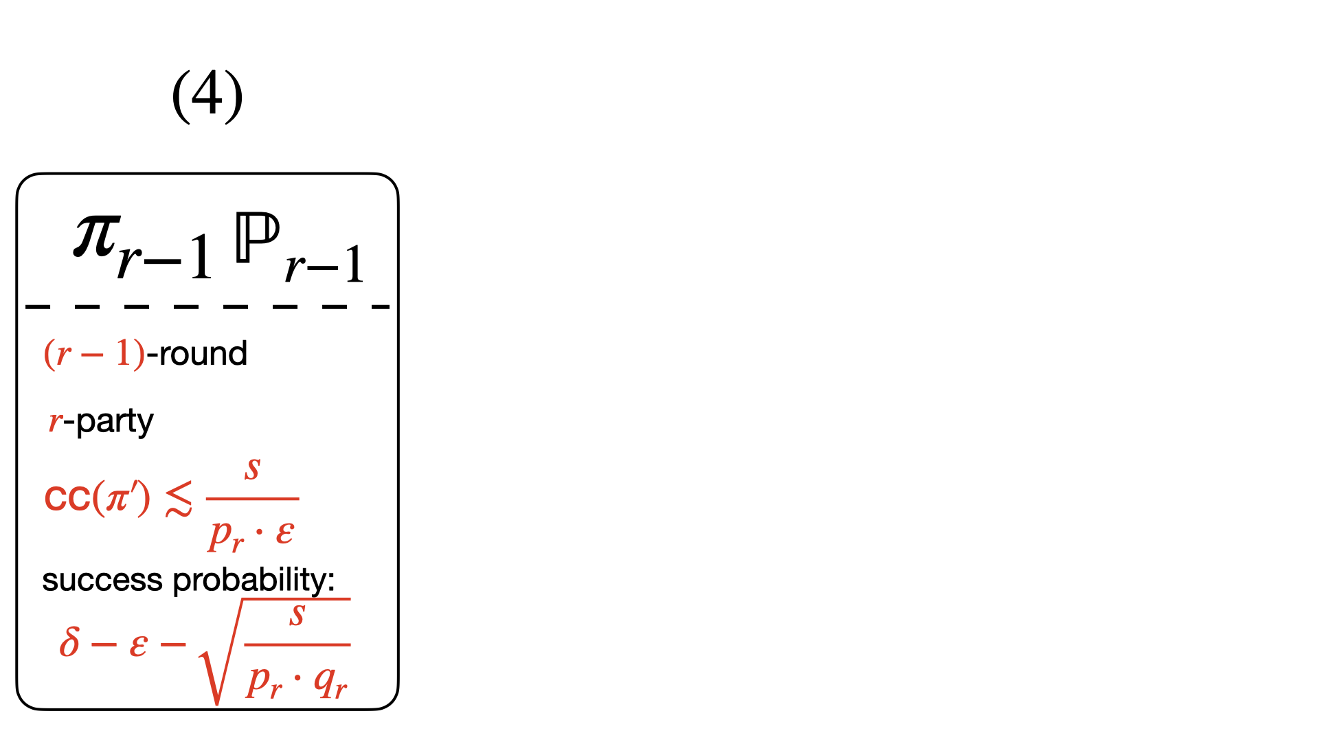
Figure 14: A schematic organization of the proof of Lemma 6.2: step 1 encompasses moving from part 1 to part 3 here, and step 2 is for moving from part 3 to part 4.

6.2 Step 1: A Low Communication Protocol for $\mathbb{P}_{r-1}$ in $r$ Rounds

Fix $r\geqslant 1$ and $n\in\mathbb{N}$ satisfying Eq 3 and let $n_{r-1}$ be determined from $n$ as in Eq 6. Suppose we have an instance $G_{r-1}$ sampled from $\mathcal{G}_{r-1}(n_{r-1})$, and we want to use $\pi_{r}$, which is for $\mathcal{G}_{r}(n)$, to solve $\mathbb{P}_{r-1}$ for all search sequences $K$ (note that we use $K$ to denote search sequences for $\mathbb{P}_{r-1}$ and not $\mathbb{P}_{r}$). Consider the following direct way of doing this:

An $r$-round $r$-party protocol $\sigma$ for $\mathbb{P}_{r-1}$ on input graph $G_{r-1}(n_{r-1})$: 1. Sample indices $k^{\star}\in[p_{r}]$ and $t\in[q_{r}]$ uniformly at random using public randomness. 2. For every $a\in[r]$, each player ${Q}_{a}$ samples $\Big{(}G_{r,a}\sim\mathcal{G}_{r}\mid{\mathsf{t}}=t,{\mathsf{H}}_{t,k^{\star},a}=G_{r-1,a}\Big{)}$ using private randomness. Let $G_{r}=(G_{r,1},G_{r,2},\ldots,G_{r,r+1})$ be the input of all players in $\mathcal{G}_{r}$ where, using Property 1, the input of the “simulated” player ${Q}_{r+1}$ is fixed by ${\mathsf{t}}=t$. 3. The players run $\pi_{r}(G_{r})$ by simulating the messages of player ${Q}_{r+1}$ in $\pi_{r}$ given that $t$ is public knowledge. 4. At the end, for any search sequence $K=(k_{r-1},\ldots,k_{1})$, to solve $\mathbb{P}_{r-1}(G_{r-1},K)$, we return the answer of $\pi_{r}$ for $\mathbb{P}_{r}(G_{r},(k^{\star},k_{r-1},k_{r-2},\ldots,k_{1}))$.

Define the distribution $\mathcal{G}^{\textnormal{{real}}}$ as the distribution of the graph $G_{r}$ obtained in the protocol $\sigma$ when $G_{r-1}\sim\mathcal{G}_{r-1}$. We claim that this is the “right” distribution.

Observation 6.3.

Distribution $\mathcal{G}^{\textnormal{{real}}}$ is the same as $\mathcal{G}_{r}$.

Proof.

We know from Property 2 that $\mathcal{G}_{r}$ is a product distribution of $\mathcal{G}_{r,1}\times\ldots\mathcal{G}_{r,r+1}$. Moreover, each $\mathcal{G}_{r,a}$ for $a\in[r]$ is, by Property 1, a collection of independent instances $H_{i,j,a}\sim\mathcal{G}_{r-1,a}$ and $t\in[q_{r}]$ is chosen uniformly at random in $\mathcal{G}_{r}$ to define the input of player ${Q}_{r+1}$. This matches exactly the distribution of $\mathcal{G}^{\textnormal{{real}}}$ in $\sigma$, given that $G_{r-1,a}$ used by player ${Q}_{a}$ is sampled from $\mathcal{G}_{r-1,a}$ by definition.       

As protocol $\pi_{r}$ can solve $\mathbb{P}_{r}$, the transcript of $\pi_{r}$ can determine $\mathbb{P}_{r}(G_{r},(k^{\star},k_{r-1},\ldots,k_{1}))$ for every $K=(k_{r-1},\ldots,k_{1})$ and any $k^{\star}\in[p_{r}]$. By 6.3, we know that the probability of success of $\sigma$ in solving $\mathbb{P}_{r-1}$ is the same as that of $\pi_{r}$ for solving $\mathbb{P}_{r}$ and is thus at least $\delta$ by the statement of Lemma 6.2.

It seems however that we have done nothing yet: $\sigma$ is a $r$-round protocol with the same communication cost as $\pi_{r}$, so effectively we made no progress. The silver lining is that we can actually prove $\sigma$ has a much lower information cost compared to $\pi_{r}$, using a direct-sum style argument.

Claim 6.4.

The information cost of protocol $\sigma$ on the distribution $\mathcal{G}_{r-1}$ is at most

$$\textsc{IC}(\sigma,\mathcal{G}_{r-1})\leqslant\frac{1}{p_{r}}\cdot\textsc{IC}(\pi,\mathcal{G}_{r}).$$

Proof.

Let ${\mathsf{k}}$ denote the random variable for the index $k^{\star}$ in $\sigma$ and ${\mathsf{\Pi}}$ denote both the messages of players in $\sigma$ as well as $\pi_{r}$ – this is because, the players in $\sigma$ communicate exactly the same messages as $\pi_{r}$ (without loss of generality, we can assume ${Q}_{r}$ also writes the message of ${Q}_{r+1}$ on the board, even though all players can calculate that message on their own also). And, by 6.3, we obtain that these messages are also distributed exactly the same way as $\pi_{r}$ is a deterministic function of the samples from $\mathcal{G}_{r}=\mathcal{G}^{\textnormal{{real}}}$. Moreover, since $\pi_{r}$ is a deterministic protocol, the only public randomness of $\sigma$ is ${\mathsf{k}}$ and ${\mathsf{t}}$. Thus,

$$\textsc{IC}(\sigma,\mathcal{G}_{r-1}) =\mathbb{I}({\mathsf{G}}_{r-1}\,;{\mathsf{\Pi}}\mid{\mathsf{k}},{\mathsf{t}})$$ (by 3.3)

$$=\sum_{k=1}^{p_{r}}\frac{1}{p_{r}}\cdot\mathbb{I}({\mathsf{H}}_{{\mathsf{t}},k}\,;{\mathsf{\Pi}}\mid{\mathsf{t}},{\mathsf{k}}=k) {\mathsf{k}} G_{r-1}=H_{t,k} \sigma t\in[q_{r}]$$ (by the distribution of and since in for any choice of )

$$=\sum_{k=1}^{p_{r}}\frac{1}{p_{r}}\cdot\mathbb{I}({\mathsf{H}}_{{\mathsf{t}},k}\,;{\mathsf{\Pi}}\mid{\mathsf{t}}),$$ (9)

where the final equality holds because of the following: the joint distribution of $({\mathsf{H}}_{{\mathsf{t}},k},{\mathsf{\Pi}},{\mathsf{t}})$ is a deterministic function of the choice of ${\mathsf{G}}_{r}\sim\mathcal{G}^{\textnormal{{real}}}$ as fixing the graph $G_{r}$ also fixes the sub-instance $H_{t,k}$ (where $t$ is the index of the special UPC of $G_{r}$) as well as all the messages of protocol $\pi_{r}=\pi_{r}(G_{r})$ which is deterministic. On the other hand, even given a fixed choice of $G_{r}$, we can still pick ${\mathsf{k}}$ uniformly at random from $[p_{r}]$ as it is entirely independent of $G_{r}$. Thus, the joint distribution of $({\mathsf{H}}_{{\mathsf{t}},k},{\mathsf{\Pi}},{\mathsf{t}})$ is independent of the event ${\mathsf{k}}=k$ and we can drop the conditioning.

The next observation is that for every $k\in[p_{r}]$, we have ${\mathsf{H}}_{{\mathsf{t}},k}\perp{\mathsf{H}}_{{\mathsf{t}},<k}\mid{\mathsf{t}}$ because the sub-instances are sampled independently and, after conditioning on ${\mathsf{t}}$, the choice of ${\mathsf{H}}_{{\mathsf{t}},k}$ and ${\mathsf{H}}_{{\mathsf{t}},<k}$ only depend on the sub-instances. Thus, we can apply Proposition A.2 to each of the mutual information terms above and get:

$$\sum_{k=1}^{p_{r}}\mathbb{I}({\mathsf{H}}_{{\mathsf{t}},k}\,;{\mathsf{\Pi}}\mid{\mathsf{t}}) \leqslant\sum_{k=1}^{p_{r}}\mathbb{I}({\mathsf{H}}_{{\mathsf{t}},k}\,;{\mathsf{\Pi}}\mid{\mathsf{t}},{\mathsf{H}}_{{\mathsf{t}},<k})$$

$$=\mathbb{I}({\mathsf{H}}_{{\mathsf{t}},*}\,;{\mathsf{\Pi}}\mid{\mathsf{t}})$$ (by the chain rule of mutual information in A.1-(4))

$$\leqslant\mathbb{I}({\mathsf{H}}_{{\mathsf{t}},*}\,;{\mathsf{\Pi}}\mid{\mathsf{t}})+\mathbb{I}({\mathsf{H}}_{-{\mathsf{t}},*}\,;{\mathsf{\Pi}}\mid{\mathsf{H}}_{{\mathsf{t}},*},{\mathsf{t}})+\mathbb{I}({\mathsf{t}}\,;{\mathsf{\Pi}})$$ (as mutual information is non-negative (A.1-(2)))

$$=\mathbb{I}(\left\{{\mathsf{H}}_{i,j}\right\}_{i\in[q_{r}],j\in[p_{r}]},{\mathsf{t}}\,;{\mathsf{\Pi}})$$ (by the chain rule of mutual information in A.1-(4))

$$=\mathbb{I}({\mathsf{G}}_{r}\,;{\mathsf{\Pi}}) G_{r} \left\{H_{i,j}\right\}_{i,j},T$$ (as fixes and vice-versa by Property 1)

$$=\textsc{IC}(\pi_{r},\mathcal{G}_{r}).$$ (by 3.3)

Plugging in this bound in Eq 9, we conclude that,

$$\textsc{IC}(\sigma,\mathcal{G}_{r-1})\leqslant\frac{1}{p_{r}}\cdot\textsc{IC}(\pi_{r},\mathcal{G}_{r}).\nobreak\hskip 0.0pt\hskip 15.00002pt minus 5.0pt\nobreak\vrule height=7.5pt,width=5.0pt,depth=2.5pt$$

We are not done however as in the next step, we really need the communication cost of the protocol to be small and not only its information cost (see 3). We do this by “compressing” the messages of $\sigma$ down to their information cost. This part uses standard ideas except for the fact that we are applying them to a multi-party protocol instead of their typical two-party application.

In the following, we design a protocol $\overline{\sigma}$ by compressing the messages of $\sigma$ on an input $G_{r-1}\sim\mathcal{G}_{r-1}$ down to their information cost. To avoid ambiguity, here, for every $a\in[r]$ and $i\in[r]$, we use $\Sigma_{i,a}$ to denote the message sent by player ${Q}_{a}$ of $\sigma$ in round $i$. We also use ${\mathsf{R}}_{\sigma}$ to denote the public randomness of $\sigma$. We define $\overline{\Sigma}_{i,a}$ and ${\mathsf{R}}_{\overline{\sigma}}$ analogously for $\overline{\sigma}$. Protocol $\overline{\sigma}$ is as follows: A communication efficient implementation of $\sigma$ as a protocol $\overline{\sigma}$: • For $i=1$ to $r$ rounds and $a=1$ to $r$ players in this order: 1. Suppose the players at this point all know $R_{\sigma}$ as well as $$\Sigma_{<i}:=\Sigma_{<i,r},\ldots,\Sigma_{<i,r},\quad\text{and}\quad\Sigma_{i,<a}:=\Sigma_{i,1},\ldots,\Sigma_{i,a-1},$$ i.e., the public randomness of $\sigma$ and the messages that “should have been” communicated by $\sigma$ in the first $i-1$ rounds plus the ones by ${Q}_{1},\ldots,{Q}_{a-1}$ in round $i$. 2. Define the distributions $$\mathcal{A}_{i,a}:={\mathsf{\Sigma}}_{i,a}\mid\Sigma_{<i},\Sigma_{i,<a},R_{\sigma},G_{r-1,a},\quad\text{and}\quad\mathcal{B}_{i,a}:={\mathsf{\Sigma}}_{i,a}\mid\Sigma_{<i},\Sigma_{i,<a},R_{\sigma};$$ notice that the difference is only that in $\mathcal{A}_{i,a}$ we also condition on the input of player ${Q}_{a}$ in $G_{r-1}$, i.e., $G_{r-1,a}$ but in $\mathcal{B}_{i,a}$, we do not. 3. The player ${Q}_{a}$ plays the role of Alice in Proposition 3.5, who knows both $\mathcal{A}_{i,a}$ and $\mathcal{B}_{i,a}$ and all other players play the role of Bob who only knows $\mathcal{B}_{i,a}$. The players use public randomness and Alice (i.e., player ${Q}_{a}$) writes the message of Proposition 3.5, denoted by $\overline{\sigma}_{i,a}$, on the blackboard which allows all players to sample a single message $$\Sigma_{i,a}\sim\mathcal{A}_{i,a}={\mathsf{\Sigma}}_{i,a}\mid\Sigma_{<i},\Sigma_{i,<a},G_{r-1,a},R_{\sigma}.$$ This allows the players to obtain the message $\Sigma_{i}(a)$ and continue this for-loop.

The fact that $\overline{\sigma}$ is faithfully simulating the protocol $\sigma$ follows immediately from Proposition 3.5 as the message compression approach has no error. We now bound the length of messages communicated by $\overline{\sigma}$ in expectation.

Claim 6.5.

The expected length of the messages communicated by the protocol $\overline{\sigma}$ is at most

$$c_{\textnormal{comp}}\cdot\Big{(}\textsc{IC}(\sigma,\mathcal{G}_{r-1})+r^{2}\Big{)},$$

where $c_{\textnormal{comp}}\geqslant 1$ is an absolute constant defined in Eq 2 (derived from Proposition 3.5).

Proof.

With a slight abuse of notation, we denote $\left|{\overline{\Sigma}}\right|$ to denote the length of the messages communicated by $\overline{\sigma}$ (on a particular input and realization of randomness) and $\left|{\overline{\Sigma}_{i,a}}\right|$ for $i\in[r]$ and $a\in[r]$ as the length of the message $\overline{\Sigma}_{i,a}$. Thus, by linearity of expectation,

$$\operatorname*{{\mathbb{E}}}\left|{\overline{\Sigma}}\right|=\sum_{i=1}^{r}\sum_{a=1}^{r}\operatorname*{{\mathbb{E}}}\left|{\overline{\Sigma}_{i,a}}\right|.$$

Moreover, by Proposition 3.5, for every $i\in[r]$ and $a\in[r]$, we have,

$$\operatorname*{{\mathbb{E}}}\left|{\overline{\Sigma}_{i,a}}\right| \leqslant c_{\textnormal{comp}}\cdot\Big{(}\operatorname*{{\mathbb{E}}}_{\Sigma_{<i},\Sigma_{i,<a},G_{r-1,a},R_{\sigma}}\mathbb{D}(\mathcal{A}_{i,a}~{}||~{}\mathcal{B}_{i,a})+1\Big{)} \mathcal{A}_{i,a},\mathcal{B}_{i,a}$$ (as the distributions of Proposition 3.5 are (conditioned on the prior messages))

$$\leqslant c_{\textnormal{comp}}\cdot\Big{(}\operatorname*{{\mathbb{E}}}_{\Sigma_{<i},\Sigma_{i,<a},G_{r-1,a},R_{\sigma}}\mathbb{D}({\mathsf{\Sigma}}_{i,a}\mid\Sigma_{<i},\Sigma_{i,<a},R_{\sigma},G_{r-1,a}~{}||~{}{\mathsf{\Sigma}}_{i,a}\mid\Sigma_{<i},\Sigma_{i,<a},R_{\sigma})+1\Big{)} \mathcal{A}_{i,a},\mathcal{B}_{i,a}$$ (by the definition of )

$$=c_{\textnormal{comp}}\cdot\Big{(}\mathbb{I}({\mathsf{\Sigma}}_{i,a}\,;{\mathsf{G}}_{r-1,a}\mid{\mathsf{\Sigma}}_{<i},{\mathsf{\Sigma}}_{i,<a},{\mathsf{R}}_{\sigma})+1\Big{)}.$$ (by A.4)

Plugging these bounds in the expectation-term above implies

$$\operatorname*{{\mathbb{E}}}\left|{\overline{\Sigma}}\right| \leqslant\sum_{i=1}^{r}\sum_{a=1}^{r}c_{\textnormal{comp}}\cdot\Big{(}\mathbb{I}({\mathsf{\Sigma}}_{i,a}\,;{\mathsf{G}}_{r-1,a}\mid{\mathsf{\Sigma}}_{<i},{\mathsf{\Sigma}}_{i,<a},{\mathsf{R}}_{\sigma})+1\Big{)}$$

$$\leqslant\sum_{i=1}^{r}\sum_{a=1}^{r}c_{\textnormal{comp}}\cdot\Big{(}\mathbb{I}({\mathsf{\Sigma}}_{i,a}\,;{\mathsf{G}}\mid{\mathsf{\Sigma}}_{<i},{\mathsf{\Sigma}}_{i,<a},{\mathsf{R}}_{\sigma})+1\Big{)} {\mathsf{G}}_{r-1,a} {\mathsf{G}}_{r-1}$$ (by A.1-(5) as is a deterministic function of )

$$=c_{\textnormal{comp}}\cdot\Big{(}\mathbb{I}(\left\{{\mathsf{\Sigma}}_{i,a}\right\}_{i\in[r],a\in[r]}\,;{\mathsf{G}}\mid{\mathsf{R}}_{\sigma})+r^{2}\Big{)}$$ (by the chain rule of mutual information in A.1-(4))

$$=c_{\textnormal{comp}}\cdot\Big{(}\textsc{IC}(\sigma,\mathcal{G}_{r-1})+r^{2}\Big{)},$$

by the definition of information cost of $\sigma$ in 3.3.       

Finally, we do a basic clean up of $\overline{\sigma}$ to bound its communication cost (in worst-case, not in expectation). This step is entirely straightforward and is basically by truncating the protocol $\overline{\sigma}$ whenever a player is going to communicate more than their “budget”. We only provide the full protocol here for completeness.

Protocol $\pi^{\prime}$: the truncated version of the protocol $\overline{\sigma}$ for a given parameter $\varepsilon>0$ • Run the protocol $\overline{\sigma}$ as is. If at any point, a player is going to send a message that results in the communication cost of the protocol to become more than $$\frac{c_{\textnormal{comp}}}{\varepsilon}\cdot\Big{(}\textsc{IC}(\sigma,\mathcal{G}_{r-1})+r^{2}\Big{)},$$ terminate the protocol and return ‘fail’.

We list the properties of the protocol $\pi^{\prime}$ in the following.

Claim 6.6.

For every $\varepsilon>0$, protocol $\pi^{\prime}$ is a $r$-round $r$-party protocol for solving $\mathbb{P}_{r-1}$ on a graph $G_{r-1}\sim\mathcal{G}_{r-1}$ with probability of success at least $\delta-\varepsilon$ and communication cost

$$\textsc{CC}(\pi^{\prime})\leqslant\frac{c_{\textnormal{comp}}}{\varepsilon}\cdot\Big{(}\frac{s}{p_{r}}+r^{2}\Big{)}.$$

Proof.

The fact that $\pi^{\prime}$ is $r$-round and $r$-party is by definition. A direct application of Markov bound, plus Claim 6.5 also implies that the probability that $\pi^{\prime}$ terminates is at most $\varepsilon$. This in turn implies that the error probability of $\pi^{\prime}$ compared to that $\overline{\sigma}$ and equivalently $\sigma$ is at most $\varepsilon$ more. Thus, $\pi^{\prime}$ succeeds with probability at least $\delta-\varepsilon$. Finally,

$$\textsc{CC}(\pi^{\prime})\underset{\textnormal{(1)}}{\leqslant}\frac{1}{\varepsilon}\cdot c_{\textnormal{comp}}\cdot\Big{(}\textsc{IC}(\sigma,\mathcal{G}_{r-1})+r^{2}\Big{)}\underset{\textnormal{(2)}}{\leqslant}\frac{c_{\textnormal{comp}}}{\varepsilon}\cdot\Big{(}\frac{1}{p_{r}}\cdot\textsc{IC}(\pi_{r},\mathcal{G}_{r})+r^{2}\Big{)}\underset{\textnormal{(3)}}{\leqslant}\frac{c_{\textnormal{comp}}}{\varepsilon}\cdot\Big{(}\frac{s}{p_{r}}+r^{2}\Big{)},$$

where $(1)$ holds because of the truncation step in $\pi^{\prime}$, $(2)$ holds by Claim 6.4, and $(3)$ holds since by Proposition 3.4, $\textsc{IC}(\pi_{r},\mathcal{G}_{r})\leqslant\textsc{CC}(\pi_{r})$, which is the parameter $s$ in Lemma 6.2.       

6.3 Step 2: A Protocol for $\mathbb{P}_{r-1}$ in $(r-1)$ Rounds via Round Elimination

Up until this point, we managed to obtain a protocol $\pi^{\prime}$ which has the desired communication cost and probability of success, but the main issue remains: it still requires $r$ rounds as opposed to $(r-1)$ rounds. In the following, we try a more nuanced way of creating an $(r-1)$-round protocol $\pi_{r-1}$ which follows the same approach as $\pi^{\prime}$ but no longer uses the first round of messages of $\pi_{r}$ at all – instead, the players simply sample those messages using public randomness.

Before we proceed however, we need to establish an important property of the original protocol $\pi_{r}$ using the fact the distribution $\mathcal{G}_{r}$ is a product distribution.

Conditional Independence of Inputs Even After Messages

We can prove that the distribution of the inputs to the players in $\mathcal{G}_{r}$ remains a product distribution (see Property 2), even conditioned on the messages of the first round of $\pi_{r}$. This is a direct consequence of the rectangle property of protocols (and is a standard fact, which is proven here merely for completeness given we are conditioning on a subset of the input and not all of it).

Lemma 6.7.

Let $\Pi_{1}$ denote all messages of $\pi_{r}$ in the first round. For any $i\in[q_{r}]$ and $j\in[p_{r}]$,

$$\textnormal{dist}(H_{i,>j},H_{>i,*}\mid H_{i,\leqslant j},\Pi_{1},H_{<i,*})=\prod_{a=1}^{r}\textnormal{dist}(H_{i,>j,a},H_{>i,*,a}\mid H_{i,\leqslant j,a},\Pi_{1},H_{<i,*}).$$

We will first show some necessary independence of distributions before proving the lemma.

Claim 6.8.

For any $a\in[r],j\in[p_{r}]$, $i\in[q_{r}]$, and any choice of $\Pi_{1},H_{i,\leqslant j,a},H_{<i,*}$,

$${\mathsf{H}}_{i,\leqslant j,-a},{\mathsf{H}}_{i,>j,<a},{\mathsf{H}}_{>i,*,<a}\perp{\mathsf{H}}_{i,>j,a},{\mathsf{H}}_{>i,*,a}\mid\Pi_{1},H_{i,\leqslant j,a},H_{<i,*}.$$

Proof.

We will show that the following mutual information term is zero, which immediately implies the claim by A.1-(2):

$$\mathbb{I}({\mathsf{H}}_{i,\leqslant j,-a},{\mathsf{H}}_{i,>j,<a},{\mathsf{H}}_{>i,*,<a}\,;{\mathsf{H}}_{i,>j,a},{\mathsf{H}}_{>i,*,a}\mid{\mathsf{\Pi}}_{1},{\mathsf{H}}_{i,\leqslant j,a},{\mathsf{H}}_{<i,*})$$

$$\hskip 28.45274pt\leqslant\mathbb{I}({\mathsf{G}}_{r-1,-a}\,;{\mathsf{G}}_{r-1,a}\mid{\mathsf{\Pi}}_{1},{\mathsf{H}}_{i,\leqslant j,a},{\mathsf{H}}_{<i,*})$$ (by the data processing inequality of A.1-(5) and Property 1)

$$\hskip 28.45274pt=\mathbb{I}({\mathsf{G}}_{r-1,-a}\,;{\mathsf{G}}_{r-1,a}\mid{\mathsf{\Pi}}_{1,\leqslant a},{\mathsf{\Pi}}_{1,>a},{\mathsf{H}}_{i,\leqslant j,a},{\mathsf{H}}_{<i,*}) {\mathsf{\Pi}}_{1}={\mathsf{\Pi}}_{1,\leqslant a},{\mathsf{\Pi}}_{1,>a}$$ (by splitting )

$$\hskip 28.45274pt\leqslant\mathbb{I}({\mathsf{G}}_{r-1,-a}\,;{\mathsf{G}}_{r-1,a}\mid{\mathsf{\Pi}}_{1,\leqslant a},{\mathsf{H}}_{i,\leqslant j,a},{\mathsf{H}}_{<i,*}) {\mathsf{\Pi}}_{1,>a}\perp{\mathsf{G}}_{r-1,a}\mid G_{r-1,-a},\Pi_{1,\leqslant a},H_{i,\leqslant j,a},H_{<i,*} {\mathsf{\Pi}}_{1,>a}$$ (by Proposition A.3 as , and is now fixed)

$$\hskip 28.45274pt=\mathbb{I}({\mathsf{G}}_{r-1,-a}\,;{\mathsf{G}}_{r-1,a}\mid{\mathsf{\Pi}}_{1,<a},{\mathsf{\Pi}}_{1,a},{\mathsf{H}}_{i,\leqslant j,a},{\mathsf{H}}_{<i,*}) {\mathsf{\Pi}}_{1,\leqslant a}={\mathsf{\Pi}}_{1,<a},{\mathsf{\Pi}}_{1,a}$$ (by further splitting )

$$\hskip 28.45274pt\leqslant\mathbb{I}({\mathsf{G}}_{r-1,-a}\,;{\mathsf{G}}_{r-1,a}\mid{\mathsf{\Pi}}_{1,<a},{\mathsf{H}}_{i,\leqslant j,a},{\mathsf{H}}_{<i,*}) {\mathsf{\Pi}}_{1,a}\perp{\mathsf{G}}_{r-1,-a}\mid G_{r-1,a},\Pi_{1,<a},H_{i,\leqslant j,a},H_{<i,*} {\mathsf{\Pi}}_{1,a}$$ (by Proposition A.3 as , and is now fixed)

$$\hskip 28.45274pt\leqslant\mathbb{I}({\mathsf{G}}_{r-1,-a}\,;{\mathsf{G}}_{r-1,a}\mid{\mathsf{H}}_{i,\leqslant j,a},{\mathsf{H}}_{<i,*}) {\mathsf{\Pi}}_{1,<a}\perp{\mathsf{G}}_{r-1,a}\mid G_{r-1,-a},H_{i,\leqslant j,a},H_{<i,*} {\mathsf{\Pi}}_{1,<a}$$ (by Proposition A.3 as ; is now fixed)

$$\hskip 28.45274pt=0.\nobreak\hskip 0.0pt\hskip 15.00002pt minus 5.0pt\nobreak\vrule height=7.5pt,width=5.0pt,depth=2.5pt H_{i,j}$$ (by Property 2 all ’s are independent and we can apply A.1-(2))

Lemma 6.7 follows easily now.

Proof of Lemma 6.7.

We have that,

$$\textnormal{dist}(H_{i,>j},H_{>i,*}\mid H_{i,\leqslant j},\Pi_{1},H_{<i,*})$$

$$\hskip 28.45274pt=\prod_{a=1}^{r}\textnormal{dist}(H_{i,>j,a},H_{>i,*,a}\mid H_{i,>j,<a},H_{>i,*,<a},H_{i,\leqslant j},\Pi_{1},H_{<i,*})$$ (by chain rule)

$$\hskip 28.45274pt=\prod_{a=1}^{r}\textnormal{dist}(H_{i,>j,a},H_{>i,*,a}\mid H_{i,>j,<a},H_{>i,*,<a},H_{i,\leqslant j,-a},H_{i,\leqslant j,a},\Pi_{1},H_{<i,*}) H_{i,\leqslant j}=H_{i,\leqslant j,-a},H_{i,\leqslant j,a}$$ (by splitting )

$$\hskip 28.45274pt=\prod_{a=1}^{r}\textnormal{dist}(H_{i,>j,a},H_{>i,*,a}\mid\Pi_{1},H_{i,\leqslant j,a},H_{<i,*}),$$ (by Claim 6.8)

completing the proof.       

Eliminating the First Round of the Protocol $\pi_{r}$

We are now ready to proceed with designing our $(r-1)$-round $r$-party protocol $\pi_{r-1}$ for $\mathbb{P}_{r-1}$ using $\pi_{r}$ (and the intermediate protocol $\pi^{\prime}$ designed in the previous step). Recall the intermediate protocol $\sigma$ in the previous step. This protocol (and subsequent ones $\overline{\sigma}$ and $\pi^{\prime}$) consists of two separate parts: (1) an embedding part that created an entire graph $G_{r}$ from $\mathcal{G}_{r}$ by placing the input $G_{r-1}\sim\mathcal{G}_{r-1}$ as one of its special sub-instances; and, (2) a simulation part that ran the protocol $\pi_{r}$ (either directly in $\sigma$ or indirectly in $\overline{\sigma}$ and $\pi^{\prime}$) on this input. In the following, we will change the embedding part (thoroughly) but stick with the same simulation part except that we will only run those simulations from the second round onwards. Formally,

An $(r-1)$-round $r$-party protocol $\pi_{r-1}$ for $\mathbb{P}_{r-1}(G_{r-1},K)$: 1. Sample first-round messages $\Pi_{1,1},\ldots,\Pi_{1,r}$ of $\pi_{r}$ from $\mathcal{G}_{r}$ and indices $k^{\star}\in[p_{r}]$ and $t\in[q_{r}]$ uniformly at random and independently using public randomness. 2. Sample $H_{<t,*},H_{t,<k^{\star}}$ from $\mathcal{G}_{r}\mid\Pi_{1,1},\ldots,\Pi_{1,r},{\mathsf{t}}=t$ using public randomness. 3. For every $a\in[r]$, each player ${Q}_{a}$ sets $H_{t,k^{\star},a}=G_{r-1,a}$ and samples $$\Big{(}G_{r,a}\sim\mathcal{G}_{r}\mid\Pi_{1,1},\ldots,\Pi_{1,r},{\mathsf{t}}=t,H_{<t,*},H_{t,<k^{\star}},{\mathsf{H}}_{t,k^{\star},a}=G_{r-1,a}\Big{)}$$ using private randomness. Let $G_{r}=(G_{r,1},G_{r,2},\ldots,G_{r,r+1})$ be the input of all players where, using Property 1, the input of the simulated player ${Q}_{r+1}$ is fixed by ${\mathsf{t}}=t$. 4. The players run $\pi_{r}(G_{r})$ from its second round onwards, following the protocol $\pi^{\prime}$ of Claim 6.6. 5. At the end, for any search sequence $K=(k_{r-1},\ldots,k_{1})$, to solve $\mathbb{P}_{r-1}(G_{r-1},K)$, return the answer of $\pi_{r}$ for $\mathbb{P}_{r}(G_{r},(k^{\star},k_{r-1},k_{r-2},\ldots,1))$ (which is possible given that $\pi^{\prime}$ generates the messages of $\pi_{r}(G_{r})$ implicitly).

Similar to step one and distribution $\mathcal{G}^{\textnormal{{real}}}$, we also define the distribution $\mathcal{G}^{\textnormal{{fake}}}$ as the distribution of the graph $G_{r}$ obtained in the protocol $\pi_{r-1}$ when $G_{r-1}\sim\mathcal{G}_{r-1}$. Unlike before, however, it is no longer the case that $\mathcal{G}^{\textnormal{{fake}}}$ is actually the “right” distribution of the input that $\pi_{r}$ expects; for instance, we now embedded $H_{t,k^{\star}}=G_{r-1}$ without conditioning on the messages $\Pi_{1,1},\ldots,\Pi_{1,r}$ in the protocol. In particular, we can write these distributions as the following (where the random variables on the RHS of each term is distributed according to $\mathcal{G}_{r}$):

$$\textnormal{dist}(\Pi_{1},k^{\star},G_{r}\sim\mathcal{G}^{\textnormal{{real}}}):= \left({\mathsf{\Pi}}_{1},{\mathsf{t}},{\mathsf{k}}\right)\times\left({\mathsf{H}}_{<{\mathsf{t}},*},{\mathsf{H}}_{{\mathsf{t}},<{\mathsf{k}}}\mid{\mathsf{\Pi}}_{1},{\mathsf{t}},{\mathsf{k}}\right)$$

$$\times\left({\mathsf{H}}_{{\mathsf{t}},{\mathsf{k}}}\mid{\mathsf{\Pi}}_{1},{\mathsf{t}},{\mathsf{k}},{\mathsf{H}}_{<{\mathsf{t}},*},{\mathsf{H}}_{{\mathsf{t}},<{\mathsf{k}}}\right)\times\left({\mathsf{G}}_{r}\mid{\mathsf{\Pi}}_{1},{\mathsf{t}},{\mathsf{k}},{\mathsf{H}}_{<{\mathsf{t}},*},{\mathsf{H}}_{{\mathsf{t}},<{\mathsf{k}}},{\mathsf{H}}_{{\mathsf{t}},{\mathsf{k}}}\right)$$ (10)

$$\textnormal{dist}(\Pi_{1},k^{\star},G_{r}\sim\mathcal{G}^{\textnormal{{fake}}}):= \left({\mathsf{\Pi}}_{1},{\mathsf{t}},{\mathsf{k}}\right)\times\left({\mathsf{H}}_{<{\mathsf{t}},*},{\mathsf{H}}_{{\mathsf{t}},<{\mathsf{k}}}\mid{\mathsf{\Pi}}_{1},{\mathsf{t}},{\mathsf{k}}\right)$$

$$\times\left({\mathsf{H}}_{{\mathsf{t}},{\mathsf{k}}}\right)\times\prod_{a=1}^{r}\left({\mathsf{G}}_{r,a}\mid{\mathsf{\Pi}}_{1},{\mathsf{t}},{\mathsf{k}},{\mathsf{H}}_{<{\mathsf{t}},*},{\mathsf{H}}_{{\mathsf{t}},<{\mathsf{k}}},{\mathsf{H}}_{{\mathsf{t}},{\mathsf{k}},a}\right).$$ (11)

In the above, with a slight abuse of notation, we wrote a triple $(\Pi,t,k^{\star},G_{r})\sim\mathcal{G}^{\textnormal{{real}}}$ (or $\sim\mathcal{G}^{\textnormal{{fake}}}$) to denote the joint distribution of all these variables when the input graph $G_{r}$ is sampled from $\mathcal{G}^{\textnormal{{real}}}$ versus when they are sampled from $\mathcal{G}^{\textnormal{{fake}}}$.

Nevertheless, we are going to prove that $\mathcal{G}^{\textnormal{{fake}}}$ is not that different from $\mathcal{G}^{\textnormal{{real}}}$ either. In particular, we prove the following lemma.

Lemma 6.9 (“distributions induced by $\mathcal{G}^{\textnormal{{real}}}$ and $\mathcal{G}^{\textnormal{{fake}}}$ are close”).

$$\|\textnormal{dist}(\Pi_{1},k^{\star},G_{r}\sim\mathcal{G}^{\textnormal{{real}}})-\textnormal{dist}(\Pi_{1},k^{\star},G_{r}\sim\mathcal{G}^{\textnormal{{fake}}})\|_{\mathrm{tvd}}\leqslant\sqrt{\frac{s}{2\,p_{r}\cdot q_{r}}}.$$

We will bound this difference term by term in Eq 10 and Eq 11. The first two terms are equal in both. The next, and the main, claim bounds the difference between the third terms. This is yet another application of direct-sum style arguments along the lines of Claim 6.4, although fundamentally different as we need a much stronger guarantee (that only holds for the first round of the protocol $\pi_{r}$). We emphasize that the following claim is talking about $\pi_{r}$ and not $\pi_{r-1}$ (as the variables in RHS of Eq 10 and Eq 11 are distributed according to $\pi_{r}$).

Claim 6.10.

$$\operatorname*{{\mathbb{E}}}_{{\mathsf{\Pi}}_{1},\,{\mathsf{t}},\,{\mathsf{k}},\,{\mathsf{H}}_{<t,*},\,{\mathsf{H}}_{t,<k^{\star}}}\|({\mathsf{H}}_{t,k^{\star}}\mid\Pi_{1},H_{<t,*},H_{t,<k^{\star}})-{\mathsf{H}}_{t,k^{\star}}\|_{\mathrm{tvd}}\leqslant\sqrt{\frac{s}{2\,p_{r}\cdot q_{r}}}.$$

Proof.

We follow the standard plan of bounding the KL-divergence of the above distributions and applying Pinsker’s inequality (A.7) at the end. In this lemma, all variables are with respect to the protocol $\pi_{r}$ on the distribution $\mathcal{G}_{r}$. The only exception is that of ${\mathsf{k}}$ which is chosen uniformly from $[p_{r}]$ (and is not defined explicitly in $\mathcal{G}_{r}$ beforehand).

By Property 2, the first $r$ players do not have any information about random variable ${\mathsf{t}}$, and thus their messages in the first round cannot reveal too much about all of the special sub-instances, and in particular $H_{t,k^{\star}}$. The last player knows ${\mathsf{t}}$ but has no access to any of the sub-instances, so should not be able to reveal anything about the special sub-instances. Overall, the first message cannot change the distribution of ${\mathsf{H}}_{t,k^{\star}}$, for a random chosen $t\in[q_{r}]$ and $k^{\star}\in[p_{r}]$ by much. Our proof formalizes this idea to get a bound on the KL-Divergence. In the following, we denote

$$\Pi_{1,\leqslant r}:=(\Pi_{1,1},\Pi_{1,2},\ldots,\Pi_{1,r}),$$

i.e., the first-round messages of all players except for the last one.

We claim that, for every $i\in[q_{r}]$ and $j\in[p_{r}]$,

$${\mathsf{H}}_{i,j}\perp{\mathsf{t}}=i,{\mathsf{k}}=j\mid\Pi_{1},{\mathsf{H}}_{<i,*},{\mathsf{H}}_{i,<j}\qquad\text{and}\qquad{\mathsf{H}}_{i,j}\perp{\mathsf{H}}_{<i,*},{\mathsf{H}}_{i,<j},{\mathsf{t}}=i,{\mathsf{k}}=j,$$ (12)

because in both cases, sub-instances are chosen independently in $\mathcal{G}_{r}$ from each other, as well as the special UPC selected by ${\mathsf{t}}$; the choice of ${\mathsf{k}}$ is also independent of the entire graph.

We can now use this and have,

$$\operatorname*{{\mathbb{E}}}_{{\mathsf{\Pi}}_{1},\,{\mathsf{t}},\,{\mathsf{k}},\,{\mathsf{H}}_{<t,*},\,{\mathsf{H}}_{t,<k^{\star}}}\mathbb{D}({\mathsf{H}}_{t,k^{\star}}\mid\Pi_{1},H_{<t,*},H_{t,<k^{\star}}~{}||~{}{\mathsf{H}}_{t,k^{\star}})$$

$$\hskip 28.45274pt=\operatorname*{{\mathbb{E}}}_{{\mathsf{\Pi}}_{1},\,{\mathsf{t}},\,{\mathsf{k}},\,{\mathsf{H}}_{<t,*},\,{\mathsf{H}}_{t,<k^{\star}}}\mathbb{D}({\mathsf{H}}_{t,k^{\star}}\mid\Pi_{1},H_{<t,*},H_{t,<k^{\star}},{\mathsf{t}}=t,{\mathsf{k}}=k^{\star}~{}||~{}{\mathsf{H}}_{t,k^{\star}}\mid H_{<t,*},H_{t,<k^{\star}},{\mathsf{t}}=t,{\mathsf{k}}=k^{\star})$$ (the distributions are the same by part one and part two of Eq 12, respectively)

$$\hskip 28.45274pt=\operatorname*{{\mathbb{E}}}_{{\mathsf{\Pi}}_{1,\leqslant r},\,{\mathsf{t}},\,{\mathsf{k}},\,{\mathsf{H}}_{<t,*},\,{\mathsf{H}}_{t,<k^{\star}}}\mathbb{D}({\mathsf{H}}_{t,k^{\star}}\mid\Pi_{1,\leqslant r},H_{t,<k^{\star}},{\mathsf{t}}=t,{\mathsf{k}}=k^{\star}~{}||~{}{\mathsf{H}}_{t,k^{\star}}\mid H_{<t,*},H_{t,<k^{\star}},{\mathsf{t}}=t,{\mathsf{k}}=k) \Pi_{1,r+1} t \Pi_{1,\leqslant r} {Q}_{r+1}$$ (because is fixed by and because it fixes the input of by Property 1)

$$\hskip 28.45274pt=\mathbb{I}({\mathsf{\Pi}}_{1,\leqslant r}\,;{\mathsf{H}}_{{\mathsf{t}},{\mathsf{k}}}\mid{\mathsf{H}}_{<{\mathsf{t}},*},{\mathsf{H}}_{{\mathsf{t}},<{\mathsf{k}}},{\mathsf{t}},{\mathsf{k}}).$$ (by A.4)

In words, the change in the KL-divergence of the distribution of the sub-instance $H_{t,k^{\star}}$ from its original distribution by the messages of first round is bounded by the information revealed by $\Pi_{1,\leqslant r}$ about this sub-instance.

We now bound this information term as follows:

$$\mathbb{I}({\mathsf{\Pi}}_{1,\leqslant r}\,;{\mathsf{H}}_{{\mathsf{t}},{\mathsf{k}}}\mid{\mathsf{H}}_{<{\mathsf{t}},*},{\mathsf{H}}_{{\mathsf{t}},<{\mathsf{k}}},{\mathsf{t}},{\mathsf{k}}) =\operatorname*{{\mathbb{E}}}_{{\mathsf{t}},{\mathsf{k}}}\Big{[}\mathbb{I}({\mathsf{\Pi}}_{1,\leqslant r}\,;{\mathsf{H}}_{t,k^{\star}}\mid{\mathsf{H}}_{<t,*},{\mathsf{H}}_{t,<k^{\star}},{\mathsf{t}}=t,{\mathsf{k}}=k^{\star})\Big{]}$$ (by the definition of conditional mutual information)

$$=\operatorname*{{\mathbb{E}}}_{{\mathsf{t}},{\mathsf{k}}}\Big{[}\mathbb{I}({\mathsf{\Pi}}_{1,\leqslant r}\,;{\mathsf{H}}_{t,k^{\star}}\mid{\mathsf{H}}_{<t,*},{\mathsf{H}}_{t,<k^{\star}})\Big{]} ({\mathsf{\Pi}}_{1,\leqslant r},{\mathsf{H}}_{t,k^{\star}},{\mathsf{H}}_{<t,*},{\mathsf{H}}_{t,<k^{\star}}) {\mathsf{t}},{\mathsf{k}}$$ (for the same reason as Eq 12 since are all independent of )

$$=\frac{1}{q_{r}}\cdot\frac{1}{p_{r}}\cdot\sum_{t=1}^{q_{r}}\sum_{k^{\star}=1}^{p_{r}}\mathbb{I}({\mathsf{\Pi}}_{1,\leqslant r}\,;{\mathsf{H}}_{t,k^{\star}}\mid{\mathsf{H}}_{<t,*},{\mathsf{H}}_{t,<k^{\star}}) {\mathsf{t}},{\mathsf{k}}$$ (as the distribution of both is uniform and independent of each other)

$$=\frac{1}{q_{r}\cdot p_{r}}\cdot\mathbb{I}({\mathsf{\Pi}}_{1,\leqslant r}\,;\left\{{\mathsf{H}}_{i,j}\right\}_{i\in[q_{r}],j\in[p_{r}]})$$ (by the chain rule of mutual information in A.1-(4))

$$\leqslant\frac{1}{q_{r}\cdot p_{r}}\cdot\mathbb{I}({\mathsf{\Pi}}\,;{\mathsf{G}})$$ (by the data processing inequality of A.1-(5) and Property 1 on inputs of players)

$$=\frac{1}{q_{r}\cdot p_{r}}\cdot\textsc{IC}(\pi_{r},\mathcal{G}_{r})$$ (by the definition of external information (3.3))

$$\leqslant\frac{1}{q_{r}\cdot p_{r}}\cdot\textsc{CC}(\pi_{r})$$ (by Proposition 3.4)

which is $s/(q_{r}\cdot p_{r})$ as $s$ is the total communication cost of $\pi_{r}$. We thus have,

$$\operatorname*{{\mathbb{E}}}_{{\mathsf{\Pi}}_{1},\,{\mathsf{t}},\,{\mathsf{k}},\,{\mathsf{H}}_{t,<k^{\star}},\,{\mathsf{H}}_{<t,*}}\mathbb{D}({\mathsf{H}}_{t,k^{\star}}\mid\Pi_{1},H_{t,<k^{\star}},H_{<t,*}~{}||~{}{\mathsf{H}}_{t,k^{\star}})\leqslant\frac{s}{q_{r}\cdot p_{r}}.$$ (13)

We can finish the proof as follows:

$$\operatorname*{{\mathbb{E}}}_{{\mathsf{\Pi}}_{1},\,{\mathsf{t}},\,{\mathsf{k}},\,{\mathsf{H}}_{t,<k^{\star}},\,{\mathsf{H}}_{<t,*}}\|({\mathsf{H}}_{t,k^{\star}}\mid\Pi_{1},H_{t,<k^{\star}},H_{<t,*})-{\mathsf{H}}_{t,k^{\star}}\|_{\mathrm{tvd}}$$

$$\hskip 28.45274pt\leqslant\operatorname*{{\mathbb{E}}}_{{\mathsf{\Pi}}_{1},\,{\mathsf{t}},\,{\mathsf{k}},\,{\mathsf{H}}_{t,<k^{\star}},\,{\mathsf{H}}_{<t,*}}\Big{[}\sqrt{1/2\cdot\mathbb{D}({\mathsf{H}}_{t,k^{\star}}\mid\Pi_{1},H_{t,<k^{\star}},H_{<t,*}~{}||~{}{\mathsf{H}}_{t,k^{\star}})}\Big{]}$$ (by Pinsker’s inequality of A.7)

$$\hskip 28.45274pt\leqslant\sqrt{1/2\cdot\operatorname*{{\mathbb{E}}}_{{\mathsf{\Pi}}_{1},\,{\mathsf{t}},\,{\mathsf{k}},\,{\mathsf{H}}_{t,<k^{\star}},\,{\mathsf{H}}_{<t,*}}\Big{[}\mathbb{D}({\mathsf{H}}_{t,k^{\star}}\mid\Pi_{1},H_{t,<k^{\star}},H_{<t,*}~{}||~{}{\mathsf{H}}_{t,k^{\star}})\Big{]}} \sqrt{\cdot}$$ (by Jensen’s inequality as is concave)

$$\hskip 28.45274pt\leqslant\sqrt{\frac{s}{2q_{r}\cdot p_{r}}},$$ (by Eq 13)

concluding the proof.       

In the following claim, we bound the fourth terms of Eq 10 and Eq 11 by showing those distributions are actually equivalent. This is a direct corollary of the conditional independences we established earlier in Lemma 6.7. The statement of the following claim is written in a rather indirect way, by stating the distance is zero instead of simply claiming the two distributions are equivalent, to make its application in the later part of the proof completely transparent.

Claim 6.11.

$$\hskip 162.18062pt\operatorname*{{\mathbb{E}}}_{{\mathsf{\Pi}}_{1},{\mathsf{t}},{\mathsf{k}},{\mathsf{H}}_{<{\mathsf{t}},*},{\mathsf{H}}_{{\mathsf{t}},<{\mathsf{k}}},{\mathsf{H}}_{{\mathsf{t}},{\mathsf{k}}}}$$

$$\|\left({\mathsf{G}}_{r}\mid\Pi_{1},t,k^{\star},H_{<t,*},H_{t,<k^{\star}},H_{t,k^{\star}}\right)-\prod_{a=1}^{r}\left({\mathsf{G}}_{r,a}\mid\Pi_{1},t,k^{\star},H_{<t,*},H_{t,<k^{\star}},H_{t,k^{\star},a}\right)\|_{\mathrm{tvd}}=0.$$

Proof.

The distribution of ${\mathsf{G}}_{r}$ conditioned on ${\mathsf{t}}=t,H_{<t,*},H_{t,<k^{\star}},H_{t,k^{\star}}$ is a function of sub-instances

$$\left\{{\mathsf{H}}_{t,j}\right\}_{j>k^{\star}}\qquad\text{and}\qquad\left\{{\mathsf{H}}_{i,j}\right\}_{i>t,j\in[p_{r}]};$$

this follows immediately from Property 1. Moreover, these distributions are independent of ${\mathsf{t}}=t$ even conditioned on ${\mathsf{\Pi}}_{1}$, since ${\mathsf{t}}=t$ fixes ${\mathsf{\Pi}}_{1,r+1}$ (again by Property 1) but the rest of ${\mathsf{\Pi}}_{1,\leqslant r}$ is independent of ${\mathsf{t}}=t$ – however, the sub-instances are only a function of ${\mathsf{\Pi}}_{1,\leqslant r}$ and thus remain independent of ${\mathsf{t}}=t$. Finally, ${\mathsf{k}}=k^{\star}$ is independent of the entire graph; hence, we have,

$$\left({\mathsf{G}}_{r}\mid\Pi_{1},t,k^{\star},H_{<t,*},H_{t,<k^{\star}},H_{t,k^{\star}}\right)=\left({\mathsf{H}}_{t,>k^{\star}},{\mathsf{H}}_{>t,*}\mid\Pi_{1},H_{<t,*},H_{t,<k^{\star}},H_{t,k^{\star}}\right)$$

$$\prod_{a=1}^{r}\left({\mathsf{G}}_{r,a}\mid\Pi_{1},t,k^{\star},H_{<t,*},H_{t,<k^{\star}},H_{t,k^{\star},a}\right)=\prod_{a=1}^{r}\left({\mathsf{H}}_{t,>k^{\star},a},{\mathsf{H}}_{>t,*,a}\mid\Pi_{1},H_{<t,*},H_{t,<k^{\star}},H_{t,k^{\star},a}\right).$$

The two RHS are now equal by Lemma 6.7, proving the claim.       

Lemma 6.9 now follows from Claim 6.10 and Claim 6.11 and the chain rule (upper bound) for total variation distance (A.6).

We can now conclude the proof of Lemma 6.2, by showing that the protocol $\pi_{r-1}$ can solve $\mathbb{P}_{r-1}$ with the desired probability.

Proof of Lemma 6.2.

Suppose we sample a graph $G_{r-1}\sim\mathcal{G}_{r-1}$ and run protocol $\pi^{\prime}$ of step one in Section 6.2 on this graph by creating the messages and instance $(\Pi_{1},G_{r})\sim\mathcal{G}^{\textnormal{{real}}}$; then, by Claim 6.6,

$$\operatorname*{\textnormal{Pr}}_{\begin{subarray}{c}G_{r-1}\sim\mathcal{G}_{r-1}\\ \\ (\Pi_{1},k^{\star},G_{r})\sim\mathcal{G}^{\textnormal{{real}}}\end{subarray}}\Big{(}\text{$\pi^{\prime}$ succeeds in solving $\mathbb{P}_{r-1}$}\Big{)}\geqslant\delta-\varepsilon,$$ (14)

for the parameters $\delta$ and $\varepsilon$ in the lemma’s statement.

On the other hand, what we are actually doing in $\pi_{r-1}$ is to sample $G_{r-1}\sim\mathcal{G}_{r-1}$ but then run $\pi^{\prime}$ of step one on this graph by creating messages and instance $(\Pi_{1},G_{r})\sim\mathcal{G}^{\textnormal{{fake}}}$ instead. Thus,

$$\operatorname*{\textnormal{Pr}}_{G_{r-1}\sim\mathcal{G}_{r-1}}\Big{(}\text{$\pi_{r-1}$ succeeds in solving $\mathbb{P}_{r-1}$}\Big{)}=\operatorname*{\textnormal{Pr}}_{\begin{subarray}{c}G_{r-1}\sim\mathcal{G}_{r-1}\\ \\ (\Pi_{1},k^{\star},G_{r})\sim\mathcal{G}^{\textnormal{{fake}}}\end{subarray}}\Big{(}\text{$\pi^{\prime}$ succeeds in solving $\mathbb{P}_{r-1}$}\Big{)}.$$ (15)

Nevertheless, the RHS of this equation and the LHS of the above one are quite close to each other by Lemma 6.9 so we should be able to extend the first equation to the second one as well. Formally,

$$\operatorname*{\textnormal{Pr}}_{\begin{subarray}{c}G_{r-1}\sim\mathcal{G}_{r-1}\\ \\ (\Pi_{1},k^{\star},G_{r})\sim\mathcal{G}^{\textnormal{{fake}}}\end{subarray}}\Big{(}\text{$\pi^{\prime}$ succeeds in solving $\mathbb{P}_{r-1}$}\Big{)}$$

$$\hskip 28.45274pt\geqslant\operatorname*{\textnormal{Pr}}_{\begin{subarray}{c}G_{r-1}\sim\mathcal{G}_{r-1}\\ (\Pi_{1},k^{\star},G_{r})\sim\mathcal{G}^{\textnormal{{real}}}\end{subarray}}\Big{(}\text{$\pi^{\prime}$ succeeds in solving $\mathbb{P}_{r-1}$}\Big{)}-\|{(\Pi_{1},k^{\star},G_{r})\sim\mathcal{G}^{\textnormal{{real}}}}-{(\Pi_{1},k^{\star},G_{r})\sim\mathcal{G}^{\textnormal{{fake}}}}\|_{\mathrm{tvd}}$$ (by A.5)

$$\hskip 28.45274pt\geqslant\delta-\varepsilon-\sqrt{\frac{s}{2\,p_{r}\cdot q_{r}}}.$$ (by Eq 14 for the first term and Lemma 6.9 for the second one)

Plugging in this bound in Eq 15 implies that $\pi_{r-1}$ solves $\mathbb{P}_{r-1}$ with the desired probability.

Also, again, by Claim 6.6, we have that $\pi_{r-1}$ has communication cost

$$\textsc{CC}(\pi_{r-1})\leqslant\frac{c_{\textnormal{comp}}}{\varepsilon}\cdot\Big{(}\frac{s}{p_{r}}+r^{2}\Big{)}.$$

Finally, we can fix the randomness of $\pi_{r-1}$ by an averaging argument to obtain a deterministic algorithm with the same performance. We now have the desired deterministic $(r-1)$-round $r$-party protocol for $\mathbb{P}_{r-1}$, concluding the proof.       

Remark 3.

The reason we needed the message compression arguments and the protocols $\overline{\sigma}$ and $\pi^{\prime}$ of step one, instead of working with the protocol $\sigma$ right away is the very last step of the proof above. Had we directly used $\sigma$, then, in the last step, we should have bounded the information cost of $\overline{\sigma}$ on the new distribution $\mathcal{G}^{\textnormal{{fake}}}$ instead of $\mathcal{G}^{\textnormal{{real}}}$ – while, by Lemma 6.9, these two distributions are statistically close, this does not imply that the information cost of $\overline{\sigma}$ on $\mathcal{G}^{\textnormal{{fake}}}$ will be small also, which stops us from applying the induction hypothesis.

6.4 Proof of Lemma 6.1

We now use Lemma 6.2 to complete the proof of Lemma 6.1 (restated below). At this stage, the main arguments have been made and the remainder of the proof, for the most part, is a tedious calculation based on the parameters set in Eq 6 and Eq 8.

Lemma (Restatement of Lemma 6.1).

For any $r\geqslant 1$, any $r$-round protocol $\pi$ that given $G\sim\mathcal{G}_{r}(n)$ (for $n,r$ satisfying Eq 3), can solve $\mathbb{P}_{r}$ on input graph $G$ with probability of success at least

$$2^{-p_{0}}\cdot\left(1+\frac{r}{20\cdot(r+1)}\right)$$

has communication cost

$$\textsc{CC}(\pi)\geqslant s_{r}(n):=\frac{1}{{n_{0}}^{2}\cdot(2^{p_{0}}\cdot 40\cdot c_{\textnormal{comp}})^{r}\cdot((r+1)!)^{2}\cdot e^{3r\ln^{5/6}(n)}}\cdot\left({(n)}\uparrow\left(1+\frac{1}{2^{r}-1}\right)\right).$$

Proof.

Given that there is a distribution over $G$ and we are working with communication cost (which is a worst-case measure), it suffices to prove Lemma 6.1 for deterministic protocols; the result for randomized protocols then follows immediately by the easy direction of Yao’s minimax principle (namely, by fixing the randomness of the protocol to its “best” choice using an averaging argument). We prove the lemma using induction on $r$.

Base Case.

We prove the base case when $r=1$. Assume towards a contradiction that there exists a protocol $\pi_{1}$ for $\mathcal{G}_{1}(n)$ which uses communication

$$\textsc{CC}(\pi_{1})<s_{1}(n)=\frac{1}{n_{0}^{2}\cdot(2^{p_{0}}\cdot 40c_{\textnormal{comp}})\cdot(2!)^{2}\cdot e^{3\ln^{5/6}(n)}}\cdot n^{2},$$

and success probability at least $2^{-p_{0}}\cdot 41/40$. We will use Lemma 6.2 on $\pi_{1}$ to get a $0$-round protocol.

We know that a $0$-round protocol cannot change the prior distribution of $\mathbb{P}_{0}(G,\emptyset)$ for $G\sim\mathcal{G}_{0}(n_{0})$ which is uniform over $\left\{0,1\right\}^{p_{0}}$. Thus, the probability that the $0$-round protocol can solve the predicate $\mathbb{P}_{0}$ is $2^{-p_{0}}$ as it returns a fixed answer to $\mathbb{P}_{0}(G,\emptyset)$ independent of $G$.

We use Lemma 6.2 on $\pi_{1}$ with the following parameters (from Eq 8 for $r=1$):

$$\epsilon=\frac{1}{160\cdot 2^{p_{0}}}\qquad p_{1}=\frac{2b_{1}}{\exp(\eta_{p}\cdot(\ln(2b_{1}))^{3/4})}\qquad q_{1}=\frac{2b_{1}}{\exp(\eta_{q}\cdot(\ln(2b_{1}))^{3/4})}.$$

We get a $0$-round protocol $\pi_{0}$, which cannot communicate any bits. We will just analyze the probability of success of $\pi_{0}$. We have,

$$\frac{s_{1}(n)}{p_{1}\cdot q_{1}} =\underbrace{\frac{1}{n_{0}^{2}\cdot(2^{p_{0}}\cdot 40c_{\textnormal{comp}})\cdot(2!)^{2}\cdot e^{3\ln^{5/6}(n)}}\cdot n^{2}}_{=s_{1}}\cdot\underbrace{\frac{\exp(\eta_{p}\cdot(\ln(2b_{1}))^{3/4})}{2b_{1}}}_{=1/p_{1}}\cdot\underbrace{\frac{\exp(\eta_{q}\cdot(\ln(2b_{1}))^{3/4})}{2b_{1}}}_{=1/q_{1}}$$

$$=\frac{1}{16\cdot 40\cdot 2^{p_{0}}\cdot c_{\textnormal{comp}}}\cdot\frac{(2\cdot b_{1}n_{0})^{2}}{4\cdot b_{1}^{2}\cdot n_{0}^{2}}\cdot\exp((\eta_{p}+\eta_{q})\cdot\ln^{3/4}(2b_{1})-3\ln^{5/6}(n)) b_{1}=(n/2n_{0})$$ (by choice of from Eq 4)

$$\leqslant\frac{1}{16\cdot 40\cdot 2^{p_{0}}\cdot c_{\textnormal{comp}}}\cdot\exp(-2\ln^{5/6}(n)) \eta_{p}=O(1),\eta_{q}=O(1) 2b_{1}<n O(\ln^{3/4}(n))<\ln^{5/6}(n) n$$ (as , , and for large )

$$\leqslant\left(\frac{1}{160\cdot 2^{p_{0}}}\right)^{2}.$$ (taking a loose but sufficient upper bound)

Thus, by Lemma 6.2, the probability of success of $\pi_{0}$ is at least,

$$\frac{41}{40\cdot 2^{p_{0}}}-\underbrace{\frac{1}{160\cdot 2^{p_{0}}}}_{\varepsilon}-\underbrace{\frac{1}{160\cdot 2^{p_{0}}}}_{\sqrt{s_{1}(n)/(p_{1}\cdot q_{1})}}=\frac{81}{80\cdot 2^{p_{0}}}>\frac{1}{2^{p_{0}}},$$

which is a contradiction. This proves the induction base for $r=1$.

Induction Step.

We now prove the induction step wherein we assume the statement is true for $r-1$ and we prove it for $r>1$. Suppose towards a contradiction that there exists a protocol $\pi_{r}$ with probability of success

$$\delta:=\frac{1}{2^{p_{0}}}\left(1+\frac{r}{20\cdot(r+1)}\right)$$

for solving $\mathbb{P}_{r}$ as in the lemma statement, but with communication cost $\textsc{CC}(\pi_{r})<s_{r}(n)$ for the parameter $s_{r}(n)$ in the lemma statement. Now, recall from Eq 6 and Eq 8 that any graph sampled from distribution $\mathcal{G}_{r}$ has the following parameters:

$$\begin{split}n&=2\cdot b_{r}\cdot n_{r-1}=2\cdot\left(n_{r-1}\right)\uparrow\left(\frac{2^{r}-1}{2^{r-1}-1}\right),\\ b_{r}&=\left(n_{r-1}\right)\uparrow\left(1+\frac{1}{2^{r-1}-1}\right)\\ p_{r}&=\frac{b_{r}\cdot 2^{r}}{\exp(\eta_{p}\cdot(\ln(b_{r}\cdot 2^{r}))^{3/4})}=\frac{\left(n_{r-1}\right)\uparrow\left(1+\frac{1}{2^{r-1}-1}\right)\cdot 2^{r}}{\exp\left(\eta_{p}\cdot(r\ln 2+\ln(b_{r})\right)^{3/4})},\\ q_{r}&=\frac{b_{r}\cdot 2^{r}}{\exp(\eta_{q}\cdot(\log(b_{r}\cdot 2^{r}))^{3/4})}=\frac{\left(n_{r-1}\right)\uparrow\left(1+\frac{1}{2^{r-1}-1}\right)\cdot 2^{r}}{\exp\left(\eta_{q}\cdot(r\ln 2+\log(b_{r})\right)^{3/4})}.\end{split}$$ (16)

We use Lemma 6.2 on protocol $\pi_{r}$ with parameter

$$\varepsilon:=\frac{1}{2^{p_{0}}\cdot 40\cdot(r+1)^{2}}$$

to get a protocol $\pi_{r-1}$ for $\mathbb{P}_{r-1}$ over $\mathcal{G}_{r-1}(n_{r-1})$. We want to analyze the communication cost and probability of success of this protocol. We start by getting an upper bound on $s_{r}(n)/p_{r}$.

$$\frac{s_{r}(n)}{p_{r}} =\underbrace{\frac{{{(n)}\uparrow\left(1+\frac{1}{2^{r}-1}\right)}}{n_{0}^{2}\cdot(2^{p_{0}}\cdot 40c_{\textnormal{comp}})^{r}\cdot((r+1)!)^{2}\cdot e^{3r\ln^{5/6}(n)}}}_{=s_{r}}\cdot\underbrace{\frac{\exp\left(\eta_{p}\cdot(r\ln 2+\ln(b_{r}))^{3/4}\right)}{b_{r}\cdot 2^{r}}}_{=1/p_{r}}$$

$$=\frac{2^{\frac{2^{r}}{2^{r}-1}}\cdot\left(n_{r-1}\right)\uparrow\left(\frac{2^{r}}{2^{r-1}-1}\right)}{n_{0}^{2}\cdot(2^{p_{0}}\cdot 40c_{\textnormal{comp}})^{r}\cdot((r+1)!)^{2}\cdot 2^{r}}\cdot\frac{1}{b_{r}}\cdot\exp\left(\eta_{p}\cdot(r\ln 2+\ln(b_{r}))^{3/4}-3r\ln^{5/6}(n)\right) n_{r-1} 2^{r} b_{r}$$ (by the choice of from Eq 16 and moving around the terms and in the denominator)

$$=\frac{2^{\frac{2^{r}}{2^{r}-1}}\cdot\left(n_{r-1}\right)\uparrow\left(\frac{2^{r}}{2^{r-1}-1}-\frac{2^{r-1}}{2^{r-1}-1}\right)}{n_{0}^{2}\cdot(2^{p_{0}}\cdot 40c_{\textnormal{comp}})^{r}\cdot((r+1)!)^{2}\cdot 2^{r}}\cdot\exp\left(\eta_{p}\cdot(r\ln 2+\ln(b_{r}))^{3/4}-3r\ln^{5/6}(n)\right) b_{r} n_{r-1}$$ (by the choice of from Eq 16 and writing it in the exponent of )

$$=\frac{2^{\frac{2^{r}}{2^{r}-1}}\cdot\left(n_{r-1}\right)\uparrow\left(1+\frac{1}{2^{r-1}-1}\right)}{n_{0}^{2}\cdot(2^{p_{0}}\cdot 40c_{\textnormal{comp}})^{r}\cdot((r+1)!)^{2}\cdot 2^{r}}\cdot\exp\left(\eta_{p}\cdot(r\ln 2+\ln(b_{r}))^{3/4}-3r\ln^{5/6}(n)\right) n_{r-1}$$ (by canceling the terms in the exponent of )

$$\leqslant\frac{\left(n_{r-1}\right)\uparrow\left(1+\frac{1}{2^{r-1}-1}\right)}{n_{0}^{2}\cdot(2^{p_{0}}\cdot 40c_{\textnormal{comp}})^{r}\cdot((r+1)!)^{2}\cdot 2^{r}}\cdot\exp\left(O(\ln^{3/4}(n))-3r\ln^{5/6}(n)\right) 2^{\frac{2^{r}}{2^{r}-1}}=O(1) b_{r}\leqslant n \eta_{p}=\Theta(1) r\ll\ln{n}$$ (as , by Eq 16, by Proposition 4.5, and by Eq 3)

$$\leqslant\frac{\left(n_{r-1}\right)\uparrow\left(1+\frac{1}{2^{r-1}-1}\right)}{n_{0}^{2}\cdot(2^{p_{0}}\cdot 40c_{\textnormal{comp}})^{r}\cdot((r+1)!)^{2}\cdot 2^{r}}\cdot\exp\left(-(3r-1)\ln^{5/6}(n)\right). O(\log^{3/4}(n))<\ln^{5/6}(n_{r}) n$$ (as for large )

By Lemma 6.2, the communication cost of $\pi_{r-1}$ is at most,

$$\textsc{CC}(\pi_{r-1}) \leqslant\frac{c_{\textnormal{comp}}}{\varepsilon}\cdot\left(\frac{s_{r}(n)}{p_{r}}+r^{2}\right)$$

$$\leqslant\frac{c_{\textnormal{comp}}}{\varepsilon}\cdot\left(\frac{2\cdot\left(n_{r-1}\right)\uparrow\left(1+\frac{1}{2^{r-1}-1}\right)}{n_{0}^{2}\cdot(2^{p_{0}}\cdot 40c_{\textnormal{comp}})^{r}\cdot((r+1)!)^{2}\cdot 2^{r}}\cdot\exp\left(-(3r-1)\ln^{5/6}(n)\right)\right) s_{r}(n)/p_{r} r^{2}$$ (by our bound on from above and since is (much) smaller than this bound by Eq 3 )

$$=c_{\textnormal{comp}}\cdot\underbrace{2^{p_{0}}\cdot 40\cdot(r+1)^{2}}_{=1/\varepsilon}\cdot\left(\frac{\left(n_{r-1}\right)\uparrow\left(1+\frac{1}{2^{r-1}-1}\right)}{n_{0}^{2}\cdot(2^{p_{0}}\cdot 40c_{\textnormal{comp}})^{r}\cdot((r+1)!)^{2}\cdot 2^{r-1}}\cdot\exp\left(-(3r-2)\ln^{5/6}(n)\right)\right) \varepsilon 2 2^{r}$$ (by our choice of and canceling the -term in the nominator via in the denominator)

$$=\frac{\left(n_{r-1}\right)\uparrow\left(1+\frac{1}{2^{r-1}-1}\right)}{n_{0}^{2}\cdot(2^{p_{0}}\cdot 40c_{\textnormal{comp}})^{r-1}\cdot(r!)^{2}\cdot 2^{r-1}}\cdot\exp\left(-(3r-1)\ln^{5/6}(n)\right)$$ (by canceling the extra terms via the ones in the denominator)

$$\leqslant\frac{\left(n_{r-1}\right)\uparrow\left(1+\frac{1}{2^{r-1}-1}\right)}{n_{0}^{2}\cdot(2^{p_{0}}\cdot 40c_{\textnormal{comp}})^{r-1}\cdot(r!)^{2}\cdot 2^{r-1}\cdot e^{3\cdot(r-1)\cdot\ln^{5/6}(n_{r-1})}} e^{2\ln^{5/6}(n_{r-1})} n_{r-1}<n$$ (by dropping an extra -term and using the fact )

$$=s_{r-1}(n_{r-1}).$$

Thus, the communication cost of $\pi_{r-1}$ is less than the bounds of the induction hypothesis for $r-1$.

It remains to bound the probability of success of $\pi_{r-1}$. By Lemma 6.2,

$$\operatorname*{\textnormal{Pr}}\left(\text{$\pi_{r-1}$ solves $\mathbb{P}_{r-1}$}\right) \geqslant\delta-\varepsilon-\sqrt{\frac{s_{r}(n)}{p_{r}\cdot q_{r}}}$$

$$\geqslant\frac{1}{2^{p_{0}}}\left(1+\frac{r}{20(r+1)}\right)-\frac{1}{2^{p_{0}}\cdot 40(r+1)^{2}}-\sqrt{\frac{s_{r}(n)}{p_{r}\cdot q_{r}}}. \varepsilon \delta$$ (by the choice of and earlier in the proof)

We thus only need to bound the last term to conclude the proof.

We can upper bound this last term as follows:

$$\frac{s_{r}(n)}{p_{r}\cdot q_{r}} \leqslant\frac{\left(n_{r-1}\right)\uparrow\left(1+\frac{1}{2^{r-1}-1}\right)}{n_{0}^{2}\cdot(2^{p_{0}}\cdot 40c_{\textnormal{comp}})^{r}\cdot((r+1)!)^{2}\cdot 2^{r}}\cdot\exp\left(-(3r-1)\ln^{5/6}(n)\right)\cdot\underbrace{\frac{\exp\left(\eta_{q}\cdot(r\ln 2+\ln b_{r}\right)^{3/4})}{b_{r}\cdot 2^{r}}}_{=1/q_{r}} s_{r}(n)/p_{r} q_{r}$$ (by our upper bound on established above and the choice of in Eq 16)

$$=\frac{\exp\left(-(3r-1)\ln^{5/6}(n)+\eta_{q}\cdot(r\ln 2+\ln b_{r})^{3/4}\right)}{n_{0}^{2}\cdot(2^{p_{0}}\cdot 40c_{\textnormal{comp}})^{r}\cdot((r+1)!)^{2}\cdot 2^{2r}} b_{r}=\left(n_{r-1}\right)\uparrow\left(1+\frac{1}{2^{r-1}-1}\right)$$ (by the choice of in Eq 16 and moving around the terms)

$$\leqslant\frac{\exp\left(-(3r-1)\ln^{5/6}(n)+O(\ln^{3/4}{n})\right)}{n_{0}^{2}\cdot(2^{p_{0}}\cdot 40c_{\textnormal{comp}})^{r}\cdot((r+1)!)^{2}\cdot 2^{2r}} b_{r}\leqslant n \eta_{q}=\Theta(1) r\ll\ln{n}$$ (as by Eq 16, by Proposition 4.5, and by Eq 3)

$$\leqslant\frac{\exp(-(3r-2)\ln^{5/6}(n))}{n_{0}^{2}\cdot(2^{p_{0}}\cdot 40c_{\textnormal{comp}})^{r}\cdot((r+1)!)^{2}\cdot 2^{2r}}\cdot O(\ln^{3/4}(n))<\log^{5/6}(n) n$$ (as for large )

$$\ll\left(\frac{1}{2^{p_{0}}\cdot 40\cdot(r+1)^{2}}\right)^{2}. \ln^{5/6}\gg r$$ (using a crude upper bound sufficient for the analysis using by Eq 3)

Thus, the probability that $\pi_{r-1}$ solves $\mathbb{P}_{r-1}$ is at least

$$\frac{1}{2^{p_{0}}}\left(1+\frac{r}{20(r+1)}\right)-\frac{1}{2^{p_{0}}\cdot 40(r+1)^{2}}-\frac{1}{2^{p_{0}}\cdot 40(r+1)^{2}}>\frac{1}{2^{p_{0}}}\left(1+\frac{r-1}{20r}\right).$$

But, now $\pi_{r-1}$ is a $(r-1)$-round protocol with communication cost $\textsc{CC}(\pi_{r-1})<s_{r-1}(n_{r-1})$ and probability of success strictly larger than $1/2^{p_{0}}\cdot(1+(r-1)/20r)$ which contradicts the induction hypothesis for $r-1$ (recall that by 5.2, $n_{r-1}$ and $(r-1)$ also satisfy Eq 3 and thus we can indeed apply the induction hypothesis). This implies that our choice of the protocol $\pi_{r}$ was contradictory, completing the proof.       

6.5 Concluding the Proof of Theorem 1

Theorem 1 follows from combining the results in the previous section and the following argument.

Lemma 5.5 implies that $\textnormal{{MIS}}_{n,r+1}$ is as hard as solving $\mathbb{P}_{r}(G,K)$ for $G\sim\mathcal{G}_{r}$ and every valid search sequence $K$. Lemma 6.1 then shows that, for the $r$-round protocol $\pi$ in the theorem statement, there is a lower bound of

$$\textsc{CC}(\pi)\geqslant s_{r}(n):=\frac{1}{n_{0}^{2}\cdot(2^{p_{0}}\cdot 40c_{\textnormal{comp}})^{r}\cdot((r+1)!)^{2}\cdot e^{3r\ln^{5/6}(n)}}\cdot\left((n)\uparrow\left(1+\frac{1}{2^{r}-1}\right)\right)$$

for solving $\mathbb{P}_{r}$ on an $n$-vertex input graph $G\sim\mathcal{G}_{r}(n)$ with probability of success at least

$$\frac{1}{2^{p_{0}}}\left(1+\frac{r}{20(r+1)}\right)\leqslant\frac{21}{20\cdot 2^{p_{0}}}<\frac{21}{20\cdot 2^{(n_{0}/2)-1}}$$

for any $r\geqslant 1$. We choose $n_{0}$ to be a large enough constant to handle any constant probability of success strictly larger than zero. Thus, for $\textnormal{{MIS}}_{n,r+1}$, we obtain a lower bound of

$$\Omega\Big{(}\frac{1}{2^{\Theta(r\ln^{5/6}(n))}}\cdot n^{1+1/(2^{r}-1)}\Big{)}$$

bits on the communication cost of the problem for any $r$-round protocol as long as $n\geqslant(n_{0})^{2^{r}-1}$.

This concludes the proof of Theorem 1.       

Appendix

Appendix A Background on Information Theory

We now briefly introduce some definitions and facts from information theory that are needed in this thesis. We refer the interested reader to the text by Cover and Thomas [CT06] for an excellent introduction to this field, and the proofs of the statements used in this Appendix.

For a random variable ${\mathsf{A}}$, we use $\textnormal{\text{supp}}({\mathsf{A}})$ to denote the support of ${\mathsf{A}}$ and $\textnormal{dist}({\mathsf{A}})$ to denote its distribution. When it is clear from the context, we may abuse the notation and use ${\mathsf{A}}$ directly instead of $\textnormal{dist}({\mathsf{A}})$, for example, write $A\sim{\mathsf{A}}$ to mean $A\sim\textnormal{dist}({\mathsf{A}})$, i.e., $A$ is sampled from the distribution of random variable ${\mathsf{A}}$.

• We denote the Shannon Entropy of a random variable ${\mathsf{A}}$ by $\mathbb{H}({\mathsf{A}})$, which is defined as:

  $$\mathbb{H}({\mathsf{A}}):=\sum_{A\in\textnormal{\text{supp}}({\mathsf{A}})}\operatorname*{\textnormal{Pr}}\left({\mathsf{A}}=A\right)\cdot\log{\left(1/\operatorname*{\textnormal{Pr}}\left({\mathsf{A}}=A\right)\right)}$$ (17)

• The conditional entropy of ${\mathsf{A}}$ conditioned on ${\mathsf{B}}$ is denoted by $\mathbb{H}({\mathsf{A}}\mid{\mathsf{B}})$ and defined as:

  $$\mathbb{H}({\mathsf{A}}\mid{\mathsf{B}}):=\operatorname*{{\mathbb{E}}}_{B\sim{\mathsf{B}}}\left[\mathbb{H}({\mathsf{A}}\mid{\mathsf{B}}=B)\right],$$ (18)

  where $\mathbb{H}({\mathsf{A}}\mid{\mathsf{B}}=B)$ is defined in a standard way by using the distribution of ${\mathsf{A}}$ conditioned on the event ${\mathsf{B}}=B$ in Eq (17).

• The mutual information of two random variables ${\mathsf{A}}$ and ${\mathsf{B}}$ is denoted by $\mathbb{I}({\mathsf{A}}\,;{\mathsf{B}})$ and is defined:

  $$\mathbb{I}({\mathsf{A}}\,;{\mathsf{B}}):=\mathbb{H}(A)-\mathbb{H}(A\mid B)=\mathbb{H}(B)-\mathbb{H}(B\mid A).$$ (19)

• The conditional mutual information is defined as $\mathbb{I}({\mathsf{A}}\,;{\mathsf{B}}\mid{\mathsf{C}}):=\mathbb{H}({\mathsf{A}}\mid{\mathsf{C}})-\mathbb{H}({\mathsf{A}}\mid{\mathsf{B}},{\mathsf{C}})$.

A.1 Useful Properties of Entropy and Mutual Information

We shall use the following basic properties of entropy and mutual information throughout. Proofs of these properties mostly follow from convexity of the entropy function and Jensen’s inequality and can be found in [CT06, Chapter 2].

Fact A.1.

Let ${\mathsf{A}}$, ${\mathsf{B}}$, ${\mathsf{C}}$, and ${\mathsf{D}}$ be four (possibly correlated) random variables.

1. $0\leqslant\mathbb{H}({\mathsf{A}})\leqslant\log{\left|{\textnormal{\text{supp}}({\mathsf{A}})}\right|}$. The right equality holds iff $\textnormal{dist}({\mathsf{A}})$ is uniform.

2. $\mathbb{I}({\mathsf{A}}\,;{\mathsf{B}}\mid{\mathsf{C}})\geqslant 0$. The equality holds iff ${\mathsf{A}}$ and ${\mathsf{B}}$ are independent conditioned on ${\mathsf{C}}$.

3. Conditioning on a random variable reduces entropy: $\mathbb{H}({\mathsf{A}}\mid{\mathsf{B}},{\mathsf{C}})\leqslant\mathbb{H}({\mathsf{A}}\mid{\mathsf{B}})$. The equality holds iff ${\mathsf{A}}\perp{\mathsf{C}}\mid{\mathsf{B}}$.

4. Chain rule for mutual information: $\mathbb{I}({\mathsf{A}},{\mathsf{B}}\,;{\mathsf{C}}\mid{\mathsf{D}})=\mathbb{I}({\mathsf{A}}\,;{\mathsf{C}}\mid{\mathsf{D}})+\mathbb{I}({\mathsf{B}}\,;{\mathsf{C}}\mid{\mathsf{A}},{\mathsf{D}})$.

5. Data processing inequality: for a function $f({\mathsf{A}})$ of ${\mathsf{A}}$, $\mathbb{I}(f({\mathsf{A}})\,;{\mathsf{B}}\mid{\mathsf{C}})\leqslant\mathbb{I}({\mathsf{A}}\,;{\mathsf{B}}\mid{\mathsf{C}})$.

We also use the following two standard propositions on effect of conditioning on mutual information.

Proposition A.2.

For random variables ${\mathsf{A}},{\mathsf{B}},{\mathsf{C}},{\mathsf{D}}$, if ${\mathsf{A}}\perp{\mathsf{D}}\mid{\mathsf{C}}$, then,

$$\mathbb{I}({\mathsf{A}}\,;{\mathsf{B}}\mid{\mathsf{C}})\leqslant\mathbb{I}({\mathsf{A}}\,;{\mathsf{B}}\mid{\mathsf{C}},{\mathsf{D}}).$$

Proof.

Since ${\mathsf{A}}$ and ${\mathsf{D}}$ are independent conditioned on ${\mathsf{C}}$, by A.1-(3), $\mathbb{H}({\mathsf{A}}\mid{\mathsf{C}})=\mathbb{H}({\mathsf{A}}\mid{\mathsf{C}},{\mathsf{D}})$ and $\mathbb{H}({\mathsf{A}}\mid{\mathsf{C}},{\mathsf{B}})\geqslant\mathbb{H}({\mathsf{A}}\mid{\mathsf{C}},{\mathsf{B}},{\mathsf{D}})$. We have,

$$\mathbb{I}({\mathsf{A}}\,;{\mathsf{B}}\mid{\mathsf{C}}) =\mathbb{H}({\mathsf{A}}\mid{\mathsf{C}})-\mathbb{H}({\mathsf{A}}\mid{\mathsf{C}},{\mathsf{B}})=\mathbb{H}({\mathsf{A}}\mid{\mathsf{C}},{\mathsf{D}})-\mathbb{H}({\mathsf{A}}\mid{\mathsf{C}},{\mathsf{B}})$$

$$\leqslant\mathbb{H}({\mathsf{A}}\mid{\mathsf{C}},{\mathsf{D}})-\mathbb{H}({\mathsf{A}}\mid{\mathsf{C}},{\mathsf{B}},{\mathsf{D}})=\mathbb{I}({\mathsf{A}}\,;{\mathsf{B}}\mid{\mathsf{C}},{\mathsf{D}}).\nobreak\hskip 0.0pt\hskip 15.00002pt minus 5.0pt\nobreak\vrule height=7.5pt,width=5.0pt,depth=2.5pt$$

 

Proposition A.3.

For random variables ${\mathsf{A}},{\mathsf{B}},{\mathsf{C}},{\mathsf{D}}$, if ${\mathsf{A}}\perp{\mathsf{D}}\mid{\mathsf{B}},{\mathsf{C}}$, then,

$$\mathbb{I}({\mathsf{A}}\,;{\mathsf{B}}\mid{\mathsf{C}})\geqslant\mathbb{I}({\mathsf{A}}\,;{\mathsf{B}}\mid{\mathsf{C}},{\mathsf{D}}).$$

Proof.

Since ${\mathsf{A}}\perp{\mathsf{D}}\mid{\mathsf{B}},{\mathsf{C}}$, by A.1-(3), $\mathbb{H}({\mathsf{A}}\mid{\mathsf{B}},{\mathsf{C}})=\mathbb{H}({\mathsf{A}}\mid{\mathsf{B}},{\mathsf{C}},{\mathsf{D}})$. Moreover, since conditioning can only reduce the entropy (again by A.1-(3)),

$$\mathbb{I}({\mathsf{A}}\,;{\mathsf{B}}\mid{\mathsf{C}}) =\mathbb{H}({\mathsf{A}}\mid{\mathsf{C}})-\mathbb{H}({\mathsf{A}}\mid{\mathsf{B}},{\mathsf{C}})\geqslant\mathbb{H}({\mathsf{A}}\mid{\mathsf{D}},{\mathsf{C}})-\mathbb{H}({\mathsf{A}}\mid{\mathsf{B}},{\mathsf{C}})$$

$$=\mathbb{H}({\mathsf{A}}\mid{\mathsf{D}},{\mathsf{C}})-\mathbb{H}({\mathsf{A}}\mid{\mathsf{B}},{\mathsf{C}},{\mathsf{D}})=\mathbb{I}({\mathsf{A}}\,;{\mathsf{B}}\mid{\mathsf{C}},{\mathsf{D}}).\nobreak\hskip 0.0pt\hskip 15.00002pt minus 5.0pt\nobreak\vrule height=7.5pt,width=5.0pt,depth=2.5pt$$

 

A.2 Measures of Distance Between Distributions

We use two main measures of distance (or divergence) between distributions, namely the Kullback-Leibler divergence (KL-divergence) and the total variation distance.

KL-divergence.

For two distributions $\mu$ and $\nu$ over the same probability space, the Kullback-Leibler (KL) divergence between $\mu$ and $\nu$ is denoted by $\mathbb{D}(\mu~{}||~{}\nu)$ and defined as:

$$\mathbb{D}(\mu~{}||~{}\nu):=\operatorname*{{\mathbb{E}}}_{a\sim\mu}\Big{[}\log\frac{\mu(a)}{{\nu}(a)}\Big{]}.$$ (20)

We also have the following relation between mutual information and KL-divergence.

Fact A.4.

For random variables ${\mathsf{A}},{\mathsf{B}},{\mathsf{C}}$,

$$\mathbb{I}({\mathsf{A}}\,;{\mathsf{B}}\mid{\mathsf{C}})=\operatorname*{{\mathbb{E}}}_{(B,C)\sim{({\mathsf{B}},{\mathsf{C}})}}\Big{[}\mathbb{D}(\textnormal{dist}({\mathsf{A}}\mid{\mathsf{B}}=B,{\mathsf{C}}=C)~{}||~{}\textnormal{dist}({\mathsf{A}}\mid{\mathsf{C}}=C))\Big{]}.$$

Total variation distance.

We denote the total variation distance between two distributions $\mu$ and $\nu$ on the same support $\Omega$ by $\|\mu-\nu\|_{\mathrm{tvd}}$, defined as:

$$\|\mu-\nu\|_{\mathrm{tvd}}:=\max_{\Omega^{\prime}\subseteq\Omega}\left(\mu(\Omega^{\prime})-\nu(\Omega^{\prime})\right)=\frac{1}{2}\cdot\sum_{x\in\Omega}\left|{\mu(x)-\nu(x)}\right|.$$ (21)

We use the following basic properties of total variation distance.

Fact A.5.

Suppose $\mu$ and $\nu$ are two distributions for $\mathcal{E}$, then, ${\mu}(\mathcal{E})\leqslant{\nu}(\mathcal{E})+\|\mu-\nu\|_{\mathrm{tvd}}.$

We also have the following (chain-rule) bound on the total variation distance of joint variables.

Fact A.6.

For any distributions $\mu$ and $\nu$ on $n$-tuples $(X_{1},\ldots,X_{n})$,

$$\|\mu-\nu\|_{\mathrm{tvd}}\leqslant\sum_{i=1}^{n}\operatorname*{{\mathbb{E}}}_{X_{<i}\sim\mu}\|\mu(X_{i}\mid X_{<i})-\nu(X_{i}\mid X_{<i})\|_{\mathrm{tvd}}.$$

The following Pinsker’s inequality bounds the total variation distance between two distributions based on their KL-divergence,

Fact A.7 (Pinsker’s inequality).

For any distributions $\mu$ and $\nu$, $\|\mu-\nu\|_{\mathrm{tvd}}\leqslant\sqrt{\frac{1}{2}\cdot\mathbb{D}(\mu~{}||~{}\nu)}.$

Appendix B Extending Proposition 4.5 to all Graph Sizes

Recall that in the proof of Proposition 4.5, the graph $G$ constructed only exists for all integers $\ell\geqslant 1$, which does not include all large enough integers $n$ as in the statement of the proposition.

To fix this, we simply take the largest possible $G$ with fewer than $n$ vertices and pad each layer with extra vertices to have exactly $n$ vertices overall as required. This padding does not change the parameters $p$ and $q$. As such, we show that for any choice of large enough number of vertices $n$ there exists a choice of $n^{\prime}$ that is consistent with some integer $\ell$ such that $G$ exists and $n\geqslant n^{\prime}\geqslant{n}/{2^{\Theta(\sqrt{\log n})}}$. This implies a negligible loss on the bounds of $p$ and $q$ when $G$ is padded.

To that end, in the construction of $G$, we have that $d^{2}=\log\frac{n}{k+1}=d\cdot\log((k+2)\cdot\ell)$ and thus

$$\log(k\ell)\leqslant d_{\ell}\leqslant\log(3k\ell),\text{~{}and}$$ (22)

$$\log(k(\ell+1))\leqslant d_{\ell+1}\leqslant\log(3k(\ell+1))\leqslant\log(6k\ell)$$ (23)

where $d_{\ell}:=\log((k+2)\cdot\ell)$ refers to the choice of $d$ that depends only on integer $\ell$ (since $k$ is fixed). Let $n$ be as in the statement of the proposition where $n=b\cdot(k+1)$ for some large enough integer $b$ since the required DUP graph is a $(k+1)$-layered graph. Fix a choice of $\ell$ such that

$$b^{\prime}=((k+2)\cdot\ell)^{d_{\ell}}\leqslant b\leqslant((k+2)\cdot(\ell+1))^{d_{\ell+1}}$$ (24)

where $b^{\prime}$ also defines the integer $n^{\prime}=b^{\prime}\cdot(k+1)$. Then, using the bounds in Eq 22, Eq 23, and Eq 24, we have that

$$\frac{n}{n^{\prime}}=\frac{b}{b^{\prime}} \leqslant\frac{((k+2)\cdot(\ell+1))^{\log(6k\ell)}}{((k+2)\cdot\ell)^{\log(k\ell)}}\leqslant\left(1+\frac{1}{\ell}\right)^{\log(k\ell)}\cdot((k+2)\cdot(\ell+1))^{\log 6}$$

$$\leqslant\exp\left(\frac{\log(k\ell)}{\ell}\right)\cdot(6k\ell)^{3}\leqslant 2^{\Theta\left(\log(k\ell)\right)}.$$

Finally, since $(k\ell)^{\log(k\ell)}\leqslant\left((k+2)\cdot\ell\right)^{d_{\ell}}=b^{\prime}\leqslant b\leqslant n$, we have that

$$\log(k\ell)=\sqrt{\log(k\ell)^{\log(k\ell)}}\leqslant\sqrt{\log n}.$$

This concludes the proof for all graph sizes.

References

- [A22] S. Assadi. A two-pass (conditional) lower bound for semi-streaming maximum matching. In J. S. Naor and N. Buchbinder, editors, Proceedings of the 2022 ACM-SIAM Symposium on Discrete Algorithms, SODA 2022, Virtual Conference / Alexandria, VA, USA, January 9 - 12, 2022, pages 708–742. SIAM, 2022.
- [A23] S. Assadi. Recent advances in multi-pass graph streaming lower bounds. SIGACT News, 54(3):48–75, 2023.
- [A24] S. Assadi. A simple (1-)-approximation semi-streaming algorithm for maximum (weighted) matching. CoRR, abs/2307.02968. To appear in SOSA 2024, 2023.
- [AB16] A. Abboud and G. Bodwin. The 4/3 additive spanner exponent is tight. In D. Wichs and Y. Mansour, editors, Proceedings of the 48th Annual ACM SIGACT Symposium on Theory of Computing, STOC 2016, Cambridge, MA, USA, June 18-21, 2016, pages 351–361. ACM, 2016.
- [Abl93] F. M. Ablayev. Lower bounds for one-way probabilistic communication complexity. In Automata, Languages and Programming, 20nd International Colloquium, ICALP93, Lund, Sweden, July 5-9, 1993, Proceedings, pages 241–252, 1993.
- [ABR23] A. Azarmehr, S. Behnezhad, and M. Roghani. Fully dynamic matching: (2-)-approximation in polylog update time. CoRR, abs/2307.08772. To appear in SODA 2024., 2023.
- [ACG+15] K. J. Ahn, G. Cormode, S. Guha, A. McGregor, and A. Wirth. Correlation clustering in data streams. In Proceedings of the 32nd International Conference on Machine Learning, ICML 2015, Lille, France, 6-11 July 2015, pages 2237–2246, 2015.
- [ACK19a] S. Assadi, Y. Chen, and S. Khanna. Polynomial pass lower bounds for graph streaming algorithms. In Proceedings of the 51st Annual ACM SIGACT Symposium on Theory of Computing, STOC 2019, Phoenix, AZ, USA, June 23-26, 2019, pages 265–276, 2019.
- [ACK19b] S. Assadi, Y. Chen, and S. Khanna. Sublinear algorithms for ( + 1) vertex coloring. In Proceedings of the Thirtieth Annual ACM-SIAM Symposium on Discrete Algorithms, SODA 2019, San Diego, California, USA, January 6-9, 2019, pages 767–786, 2019.
- [ACN05] N. Ailon, M. Charikar, and A. Newman. Aggregating inconsistent information: ranking and clustering. In H. N. Gabow and R. Fagin, editors, Proceedings of the 37th Annual ACM Symposium on Theory of Computing, Baltimore, MD, USA, May 22-24, 2005, pages 684–693. ACM, 2005.
- [AD21] S. Assadi and A. Dudeja. Ruling sets in random order and adversarial streams. In S. Gilbert, editor, 35th International Symposium on Distributed Computing, DISC 2021, October 4-8, 2021, Freiburg, Germany (Virtual Conference), volume 209 of LIPIcs, pages 6:1–6:18. Schloss Dagstuhl - Leibniz-Zentrum für Informatik, 2021.
- [AG18] K. J. Ahn and S. Guha. Access to data and number of iterations: Dual primal algorithms for maximum matching under resource constraints. ACM Trans. Parallel Comput., 4(4):17:1–17:40, 2018.
- [AGM12] K. J. Ahn, S. Guha, and A. McGregor. Analyzing graph structure via linear measurements. In Proceedings of the Twenty-third Annual ACM-SIAM Symposium on Discrete Algorithms, SODA ’12, pages 459–467, 2012.
- [AJJ+22] S. Assadi, A. Jambulapati, Y. Jin, A. Sidford, and K. Tian. Semi-streaming bipartite matching in fewer passes and optimal space. In J. S. Naor and N. Buchbinder, editors, Proceedings of the 2022 ACM-SIAM Symposium on Discrete Algorithms, SODA 2022, Virtual Conference / Alexandria, VA, USA, January 9 - 12, 2022, pages 627–669. SIAM, 2022.
- [AKL17] S. Assadi, S. Khanna, and Y. Li. On estimating maximum matching size in graph streams. In Proceedings of the Twenty-Eighth Annual ACM-SIAM Symposium on Discrete Algorithms, SODA 2017, Barcelona, Spain, Hotel Porta Fira, January 16-19, pages 1723–1742, 2017.
- [AKLY16] S. Assadi, S. Khanna, Y. Li, and G. Yaroslavtsev. Maximum matchings in dynamic graph streams and the simultaneous communication model. In Proceedings of the Twenty-Seventh Annual ACM-SIAM Symposium on Discrete Algorithms, SODA 2016, Arlington, VA, USA, January 10-12, 2016, pages 1345–1364, 2016.
- [AKO20] S. Assadi, G. Kol, and R. Oshman. Lower bounds for distributed sketching of maximal matchings and maximal independent sets. In Y. Emek and C. Cachin, editors, PODC ’20: ACM Symposium on Principles of Distributed Computing, Virtual Event, Italy, August 3-7, 2020, pages 79–88. ACM, 2020.
- [AKZ22] S. Assadi, G. Kol, and Z. Zhang. Rounds vs communication tradeoffs for maximal independent sets. In 63rd IEEE Annual Symposium on Foundations of Computer Science, FOCS 2022, Denver, CO, USA, October 31 - November 3, 2022, pages 1193–1204. IEEE, 2022.
- [ALT21] S. Assadi, S. C. Liu, and R. E. Tarjan. An auction algorithm for bipartite matching in streaming and massively parallel computation models. In H. V. Le and V. King, editors, 4th Symposium on Simplicity in Algorithms, SOSA 2021, Virtual Conference, January 11-12, 2021, pages 165–171. SIAM, 2021.
- [AMS96] N. Alon, Y. Matias, and M. Szegedy. The space complexity of approximating the frequency moments. In STOC, pages 20–29. ACM, 1996.
- [AMS12] N. Alon, A. Moitra, and B. Sudakov. Nearly complete graphs decomposable into large induced matchings and their applications. In Proceedings of the 44th Symposium on Theory of Computing Conference, STOC 2012, New York, NY, USA, May 19 - 22, 2012, pages 1079–1090, 2012.
- [ANRW15] N. Alon, N. Nisan, R. Raz, and O. Weinstein. Welfare maximization with limited interaction. In IEEE 56th Annual Symposium on Foundations of Computer Science, FOCS 2015, Berkeley, CA, USA, 17-20 October, 2015, pages 1499–1512, 2015.
- [AOSS18] S. Assadi, K. Onak, B. Schieber, and S. Solomon. Fully dynamic maximal independent set with sublinear update time. In I. Diakonikolas, D. Kempe, and M. Henzinger, editors, Proceedings of the 50th Annual ACM SIGACT Symposium on Theory of Computing, STOC 2018, Los Angeles, CA, USA, June 25-29, 2018, pages 815–826. ACM, 2018.
- [AOSS19] S. Assadi, K. Onak, B. Schieber, and S. Solomon. Fully dynamic maximal independent set with sublinear in n update time. In T. M. Chan, editor, Proceedings of the Thirtieth Annual ACM-SIAM Symposium on Discrete Algorithms, SODA 2019, San Diego, California, USA, January 6-9, 2019, pages 1919–1936. SIAM, 2019.
- [AR20] S. Assadi and R. Raz. Near-quadratic lower bounds for two-pass graph streaming algorithms. In S. Irani, editor, 61st IEEE Annual Symposium on Foundations of Computer Science, FOCS 2020, Durham, NC, USA, November 16-19, 2020, pages 342–353. IEEE, 2020.
- [ARVX12] N. Alon, R. Rubinfeld, S. Vardi, and N. Xie. Space-efficient local computation algorithms. In Y. Rabani, editor, Proceedings of the Twenty-Third Annual ACM-SIAM Symposium on Discrete Algorithms, SODA 2012, Kyoto, Japan, January 17-19, 2012, pages 1132–1139. SIAM, 2012.
- [AS19] S. Assadi and S. Solomon. When algorithms for maximal independent set and maximal matching run in sublinear time. In C. Baier, I. Chatzigiannakis, P. Flocchini, and S. Leonardi, editors, 46th International Colloquium on Automata, Languages, and Programming, ICALP 2019, July 9-12, 2019, Patras, Greece, volume 132 of LIPIcs, pages 17:1–17:17. Schloss Dagstuhl - Leibniz-Zentrum für Informatik, 2019.
- [AS23] S. Assadi and J. Sundaresan. Hidden permutations to the rescue: Multi-pass semi-streaming lower bounds for approximate matchings. In IEEE Annual Symposium on Foundations of Computer Science, FOCS 2023, Santa Cruz, CA, USA. IEEE, 2023.
- [AW22] S. Assadi and C. Wang. Sublinear time and space algorithms for correlation clustering via sparse-dense decompositions. In M. Braverman, editor, 13th Innovations in Theoretical Computer Science Conference, ITCS 2022, January 31 - February 3, 2022, Berkeley, CA, USA, volume 215 of LIPIcs, pages 10:1–10:20. Schloss Dagstuhl - Leibniz-Zentrum für Informatik, 2022.
- [BBCR10] B. Barak, M. Braverman, X. Chen, and A. Rao. How to compress interactive communication. In L. J. Schulman, editor, Proceedings of the 42nd ACM Symposium on Theory of Computing, STOC 2010, Cambridge, Massachusetts, USA, 5-8 June 2010, pages 67–76. ACM, 2010.
- [BBD+19] S. Behnezhad, S. Brandt, M. Derakhshan, M. Fischer, M. Hajiaghayi, R. M. Karp, and J. Uitto. Massively parallel computation of matching and MIS in sparse graphs. In P. Robinson and F. Ellen, editors, Proceedings of the 2019 ACM Symposium on Principles of Distributed Computing, PODC 2019, Toronto, ON, Canada, July 29 - August 2, 2019, pages 481–490. ACM, 2019.
- [BBH+19] A. Balliu, S. Brandt, J. Hirvonen, D. Olivetti, M. Rabie, and J. Suomela. Lower bounds for maximal matchings and maximal independent sets. In D. Zuckerman, editor, 60th IEEE Annual Symposium on Foundations of Computer Science, FOCS 2019, Baltimore, Maryland, USA, November 9-12, 2019, pages 481–497. IEEE Computer Society, 2019.
- [BCMT22] S. Behnezhad, M. Charikar, W. Ma, and L. Tan. Almost 3-approximate correlation clustering in constant rounds. In 63rd IEEE Annual Symposium on Foundations of Computer Science, FOCS 2022, Denver, CO, USA, October 31 - November 3, 2022, pages 720–731. IEEE, 2022.
- [BCMT23] S. Behnezhad, M. Charikar, W. Ma, and L. Tan. Single-pass streaming algorithms for correlation clustering. In N. Bansal and V. Nagarajan, editors, Proceedings of the 2023 ACM-SIAM Symposium on Discrete Algorithms, SODA 2023, Florence, Italy, January 22-25, 2023, pages 819–849. SIAM, 2023.
- [BDH+19a] S. Behnezhad, M. Derakhshan, M. Hajiaghayi, M. Knittel, and H. Saleh. Streaming and massively parallel algorithms for edge coloring. In M. A. Bender, O. Svensson, and G. Herman, editors, 27th Annual European Symposium on Algorithms, ESA 2019, September 9-11, 2019, Munich/Garching, Germany, volume 144 of LIPIcs, pages 15:1–15:14. Schloss Dagstuhl - Leibniz-Zentrum für Informatik, 2019.
- [BDH+19b] S. Behnezhad, M. Derakhshan, M. Hajiaghayi, C. Stein, and M. Sudan. Fully dynamic maximal independent set with polylogarithmic update time. In D. Zuckerman, editor, 60th IEEE Annual Symposium on Foundations of Computer Science, FOCS 2019, Baltimore, Maryland, USA, November 9-12, 2019, pages 382–405. IEEE Computer Society, 2019.
- [Beh21] S. Behnezhad. Time-optimal sublinear algorithms for matching and vertex cover. In 62nd IEEE Annual Symposium on Foundations of Computer Science, FOCS 2021, Denver, CO, USA, February 7-10, 2022, pages 873–884. IEEE, 2021.
- [BEPS12] L. Barenboim, M. Elkin, S. Pettie, and J. Schneider. The locality of distributed symmetry breaking. In 53rd Annual IEEE Symposium on Foundations of Computer Science, FOCS 2012, New Brunswick, NJ, USA, October 20-23, 2012, pages 321–330. IEEE Computer Society, 2012.
- [BFS12] G. E. Blelloch, J. T. Fineman, and J. Shun. Greedy sequential maximal independent set and matching are parallel on average. In G. E. Blelloch and M. Herlihy, editors, 24th ACM Symposium on Parallelism in Algorithms and Architectures, SPAA ’12, Pittsburgh, PA, USA, June 25-27, 2012, pages 308–317. ACM, 2012.
- [BG14] M. Braverman and A. Garg. Public vs private coin in bounded-round information. In J. Esparza, P. Fraigniaud, T. Husfeldt, and E. Koutsoupias, editors, Automata, Languages, and Programming - 41st International Colloquium, ICALP 2014, Copenhagen, Denmark, July 8-11, 2014, Proceedings, Part I, volume 8572 of Lecture Notes in Computer Science, pages 502–513. Springer, 2014.
- [BH22] G. Bodwin and G. Hoppenworth. New additive spanner lower bounds by an unlayered obstacle product. In 63rd IEEE Annual Symposium on Foundations of Computer Science, FOCS 2022, Denver, CO, USA, October 31 - November 3, 2022, pages 778–788. IEEE, 2022.
- [BHP12] A. Berns, J. Hegeman, and S. V. Pemmaraju. Super-fast distributed algorithms for metric facility location. In A. Czumaj, K. Mehlhorn, A. M. Pitts, and R. Wattenhofer, editors, Automata, Languages, and Programming - 39th International Colloquium, ICALP 2012, Warwick, UK, July 9-13, 2012, Proceedings, Part II, volume 7392 of Lecture Notes in Computer Science, pages 428–439. Springer, 2012.
- [BRWY13a] M. Braverman, A. Rao, O. Weinstein, and A. Yehudayoff. Direct product via round-preserving compression. In F. V. Fomin, R. Freivalds, M. Z. Kwiatkowska, and D. Peleg, editors, Automata, Languages, and Programming - 40th International Colloquium, ICALP 2013, Riga, Latvia, July 8-12, 2013, Proceedings, Part I, volume 7965 of Lecture Notes in Computer Science, pages 232–243. Springer, 2013.
- [BRWY13b] M. Braverman, A. Rao, O. Weinstein, and A. Yehudayoff. Direct products in communication complexity. In 54th Annual IEEE Symposium on Foundations of Computer Science, FOCS 2013, 26-29 October, 2013, pages 746–755, 2013.
- [BS23] S. Behnezhad and M. Saneian. Streaming edge coloring with asymptotically optimal colors. CoRR, abs/2305.01714, 2023.
- [BW15] M. Braverman and O. Weinstein. An interactive information odometer and applications. In Proceedings of the Forty-Seventh Annual ACM on Symposium on Theory of Computing, STOC 2015, June 14-17, 2015, pages 341–350, 2015.
- [CCM08] A. Chakrabarti, G. Cormode, and A. McGregor. Robust lower bounds for communication and stream computation. In Proceedings of the 40th Annual ACM Symposium on Theory of Computing, Victoria, British Columbia, Canada, May 17-20, 2008, pages 641–650, 2008.
- [CDK14] F. Chierichetti, N. N. Dalvi, and R. Kumar. Correlation clustering in mapreduce. In S. A. Macskassy, C. Perlich, J. Leskovec, W. Wang, and R. Ghani, editors, The 20th ACM SIGKDD International Conference on Knowledge Discovery and Data Mining, KDD ’14, New York, NY, USA - August 24 - 27, 2014, pages 641–650. ACM, 2014.
- [CDK19] G. Cormode, J. Dark, and C. Konrad. Independent sets in vertex-arrival streams. In 46th International Colloquium on Automata, Languages, and Programming, ICALP 2019, July 9-12, 2019, Patras, Greece, pages 45:1–45:14, 2019.
- [CE06] D. Coppersmith and M. Elkin. Sparse sourcewise and pairwise distance preservers. SIAM J. Discret. Math., 20(2):463–501, 2006.
- [CKL+24] M. Cambus, F. Kuhn, E. Lindy, S. Pai, and J. Uitto. A -approximate correlation clustering algorithm in dynamic streams. In D. Woodruff, editor, Proceedings of the ACM-SIAM Symposium on Discrete Algorithms, SODA 2024. SIAM, 2024.
- [CKP+21a] L. Chen, G. Kol, D. Paramonov, R. R. Saxena, Z. Song, and H. Yu. Almost optimal super-constant-pass streaming lower bounds for reachability. In S. Khuller and V. V. Williams, editors, STOC ’21: 53rd Annual ACM SIGACT Symposium on Theory of Computing, Virtual Event, Italy, June 21-25, 2021, pages 570–583. ACM, 2021.
- [CKP+21b] L. Chen, G. Kol, D. Paramonov, R. R. Saxena, Z. Song, and H. Yu. Near-optimal two-pass streaming algorithm for sampling random walks over directed graphs. In N. Bansal, E. Merelli, and J. Worrell, editors, 48th International Colloquium on Automata, Languages, and Programming, ICALP 2021, July 12-16, 2021, Glasgow, Scotland (Virtual Conference), volume 198 of LIPIcs, pages 52:1–52:19. Schloss Dagstuhl - Leibniz-Zentrum für Informatik, 2021.
- [CKPU23] M. Cambus, F. Kuhn, S. Pai, and J. Uitto. Time and space optimal massively parallel algorithm for the 2-ruling set problem. CoRR, abs/2306.00432, 2023.
- [CLM+21] V. Cohen-Addad, S. Lattanzi, S. Mitrovic, A. Norouzi-Fard, N. Parotsidis, and J. Tarnawski. Correlation clustering in constant many parallel rounds. In M. Meila and T. Zhang, editors, Proceedings of the 38th International Conference on Machine Learning, ICML 2021, 18-24 July 2021, Virtual Event, volume 139 of Proceedings of Machine Learning Research, pages 2069–2078. PMLR, 2021.
- [CMZ23] S. Chechik, D. Mukhtar, and T. Zhang. Streaming edge coloring with subquadratic palette size. CoRR, abs/2305.07090, 2023.
- [CSWY01] A. Chakrabarti, Y. Shi, A. Wirth, and A. C. Yao. Informational complexity and the direct sum problem for simultaneous message complexity. In 42nd Annual Symposium on Foundations of Computer Science, FOCS 2001, 14-17 October 2001, Las Vegas, Nevada, USA, pages 270–278. IEEE Computer Society, 2001.
- [CT06] T. M. Cover and J. A. Thomas. Elements of information theory (2. ed.). Wiley, 2006.
- [CZ19] S. Chechik and T. Zhang. Fully dynamic maximal independent set in expected poly-log update time. In D. Zuckerman, editor, 60th IEEE Annual Symposium on Foundations of Computer Science, FOCS 2019, Baltimore, Maryland, USA, November 9-12, 2019, pages 370–381. IEEE Computer Society, 2019.
- [Dar20] J. Dark. Finding structure in data streams: correlations, independent sets, and matchings. PhD thesis, University of Warwick, 2020.
- [DKO14] A. Drucker, F. Kuhn, and R. Oshman. On the power of the congested clique model. In M. M. Halldórsson and S. Dolev, editors, ACM Symposium on Principles of Distributed Computing, PODC ’14, Paris, France, July 15-18, 2014, pages 367–376. ACM, 2014.
- [FGH+24] M. Flin, M. Ghaffari, M. M. Halldórsson, F. Kuhn, and A. Nolin. A distributed palette sparsification theorem. In D. Woodruff, editor, Proceedings of the ACM-SIAM Symposium on Discrete Algorithms, SODA 2024. SIAM, 2024.
- [FKM+05] J. Feigenbaum, S. Kannan, A. McGregor, S. Suri, and J. Zhang. On graph problems in a semi-streaming model. Theor. Comput. Sci., 348(2-3):207–216, 2005.
- [FN18] M. Fischer and A. Noever. Tight analysis of parallel randomized greedy MIS. In A. Czumaj, editor, Proceedings of the Twenty-Ninth Annual ACM-SIAM Symposium on Discrete Algorithms, SODA 2018, New Orleans, LA, USA, January 7-10, 2018, pages 2152–2160. SIAM, 2018.
- [GG23] M. Ghaffari and C. Grunau. Faster deterministic distributed MIS and approximate matching. In B. Saha and R. A. Servedio, editors, Proceedings of the 55th Annual ACM Symposium on Theory of Computing, STOC 2023, Orlando, FL, USA, June 20-23, 2023, pages 1777–1790. ACM, 2023.
- [GGK+18] M. Ghaffari, T. Gouleakis, C. Konrad, S. Mitrovic, and R. Rubinfeld. Improved massively parallel computation algorithms for mis, matching, and vertex cover. In Proceedings of the 2018 ACM Symposium on Principles of Distributed Computing, PODC 2018, July 23-27, 2018, pages 129–138, 2018.
- [Gha16] M. Ghaffari. An improved distributed algorithm for maximal independent set. In R. Krauthgamer, editor, Proceedings of the Twenty-Seventh Annual ACM-SIAM Symposium on Discrete Algorithms, SODA 2016, Arlington, VA, USA, January 10-12, 2016, pages 270–277. SIAM, 2016.
- [Gha22] M. Ghaffari. Local computation of maximal independent set. In 63rd IEEE Annual Symposium on Foundations of Computer Science, FOCS 2022, Denver, CO, USA, October 31 - November 3, 2022, pages 438–449. IEEE, 2022.
- [GKK12] A. Goel, M. Kapralov, and S. Khanna. On the communication and streaming complexity of maximum bipartite matching. In Y. Rabani, editor, Proceedings of the Twenty-Third Annual ACM-SIAM Symposium on Discrete Algorithms, SODA 2012, Kyoto, Japan, January 17-19, 2012, pages 468–485. SIAM, 2012.
- [GM08] S. Guha and A. McGregor. Tight lower bounds for multi-pass stream computation via pass elimination. In L. Aceto, I. Damgård, L. A. Goldberg, M. M. Halldórsson, A. Ingólfsdóttir, and I. Walukiewicz, editors, Automata, Languages and Programming, 35th International Colloquium, ICALP 2008, Reykjavik, Iceland, July 7-11, 2008, Proceedings, Part I: Tack A: Algorithms, Automata, Complexity, and Games, volume 5125 of Lecture Notes in Computer Science, pages 760–772. Springer, 2008.
- [GO16] V. Guruswami and K. Onak. Superlinear lower bounds for multipass graph processing. Algorithmica, 76(3):654–683, 2016.
- [GS23] P. Ghosh and M. Stoeckl. Low-memory algorithms for online and w-streaming edge coloring. CoRR, abs/2304.12285, 2023.
- [GU19] M. Ghaffari and J. Uitto. Sparsifying distributed algorithms with ramifications in massively parallel computation and centralized local computation. In T. M. Chan, editor, Proceedings of the Thirtieth Annual ACM-SIAM Symposium on Discrete Algorithms, SODA 2019, San Diego, California, USA, January 6-9, 2019, pages 1636–1653. SIAM, 2019.
- [Hes03] W. Hesse. Directed graphs requiring large numbers of shortcuts. In Proceedings of the Fourteenth Annual ACM-SIAM Symposium on Discrete Algorithms, January 12-14, 2003, Baltimore, Maryland, USA, pages 665–669. ACM/SIAM, 2003.
- [HJMR07] P. Harsha, R. Jain, D. A. McAllester, and J. Radhakrishnan. The communication complexity of correlation. In 22nd Annual IEEE Conference on Computational Complexity (CCC 2007), 13-16 June 2007, San Diego, California, USA, pages 10–23. IEEE Computer Society, 2007.
- [HP21] S. Huang and S. Pettie. Lower bounds on sparse spanners, emulators, and diameter-reducing shortcuts. SIAM J. Discret. Math., 35(3):2129–2144, 2021.
- [HZ23] A. Haqi and H. Zarrabi-Zadeh. Almost optimal massively parallel algorithms for k-center clustering and diversity maximization. In K. Agrawal and J. Shun, editors, Proceedings of the 35th ACM Symposium on Parallelism in Algorithms and Architectures, SPAA 2023, Orlando, FL, USA, June 17-19, 2023, pages 239–247. ACM, 2023.
- [JRS09] R. Jain, J. Radhakrishnan, and P. Sen. A property of quantum relative entropy with an application to privacy in quantum communication. J. ACM, 56(6):33:1–33:32, 2009.
- [Kap13] M. Kapralov. Better bounds for matchings in the streaming model. In Proceedings of the Twenty-Fourth Annual ACM-SIAM Symposium on Discrete Algorithms, SODA 2013, New Orleans, Louisiana, USA, January 6-8, 2013, pages 1679–1697, 2013.
- [Kap21] M. Kapralov. Space lower bounds for approximating maximum matching in the edge arrival model. In D. Marx, editor, Proceedings of the 2021 ACM-SIAM Symposium on Discrete Algorithms, SODA 2021, Virtual Conference, January 10 - 13, 2021, pages 1874–1893. SIAM, 2021.
- [KMVV13] R. Kumar, B. Moseley, S. Vassilvitskii, and A. Vattani. Fast greedy algorithms in mapreduce and streaming. In 25th ACM Symposium on Parallelism in Algorithms and Architectures, SPAA ’13, Montreal, QC, Canada - July 23 - 25, 2013, pages 1–10, 2013.
- [KMW16] F. Kuhn, T. Moscibroda, and R. Wattenhofer. Local computation: Lower and upper bounds. J. ACM, 63(2):17:1–17:44, 2016.
- [KN97] E. Kushilevitz and N. Nisan. Communication complexity. Cambridge University Press, 1997.
- [KN21] C. Konrad and K. K. Naidu. On two-pass streaming algorithms for maximum bipartite matching. In M. Wootters and L. Sanità, editors, Approximation, Randomization, and Combinatorial Optimization. Algorithms and Techniques, APPROX/RANDOM 2021, August 16-18, 2021, University of Washington, Seattle, Washington, USA (Virtual Conference), volume 207 of LIPIcs, pages 19:1–19:18. Schloss Dagstuhl - Leibniz-Zentrum für Informatik, 2021.
- [KN24] C. Konrad and K. K. Naidu. An unconditional lower bound for two-pass streaming algorithms for maximum matching approximation. In Proceedings of the 2024 ACM-SIAM Symposium on Discrete Algorithms, SODA 2024. SIAM, 2024.
- [KNR95] I. Kremer, N. Nisan, and D. Ron. On randomized one-round communication complexity. In Proceedings of the Twenty-Seventh Annual ACM Symposium on Theory of Computing, 29 May-1 June 1995, Las Vegas, Nevada, USA, pages 596–605, 1995.
- [Kon18a] C. Konrad. MIS in the congested clique model in o(log log ) rounds. CoRR, abs/1802.07647, 2018.
- [Kon18b] C. Konrad. A simple augmentation method for matchings with applications to streaming algorithms. In I. Potapov, P. G. Spirakis, and J. Worrell, editors, 43rd International Symposium on Mathematical Foundations of Computer Science, MFCS 2018, August 27-31, 2018, Liverpool, UK, volume 117 of LIPIcs, pages 74:1–74:16. Schloss Dagstuhl - Leibniz-Zentrum für Informatik, 2018.
- [KPRR19] C. Konrad, S. V. Pemmaraju, T. Riaz, and P. Robinson. The complexity of symmetry breaking in massive graphs. In J. Suomela, editor, 33rd International Symposium on Distributed Computing, DISC 2019, October 14-18, 2019, Budapest, Hungary, volume 146 of LIPIcs, pages 26:1–26:18. Schloss Dagstuhl - Leibniz-Zentrum für Informatik, 2019.
- [Lin87] N. Linial. Distributive graph algorithms-global solutions from local data. In 28th Annual Symposium on Foundations of Computer Science, Los Angeles, California, USA, 27-29 October 1987, pages 331–335. IEEE Computer Society, 1987.
- [LMSV11] S. Lattanzi, B. Moseley, S. Suri, and S. Vassilvitskii. Filtering: a method for solving graph problems in mapreduce. In SPAA 2011: Proceedings of the 23rd Annual ACM Symposium on Parallelism in Algorithms and Architectures, San Jose, CA, USA, June 4-6, 2011 (Co-located with FCRC 2011), pages 85–94, 2011.
- [Lub85] M. Luby. A simple parallel algorithm for the maximal independent set problem. In Proceedings of the 17th Annual ACM Symposium on Theory of Computing, May 6-8, 1985, Providence, Rhode Island, USA, pages 1–10, 1985.
- [LWWX22] K. Lu, V. V. Williams, N. Wein, and Z. Xu. Better lower bounds for shortcut sets and additive spanners via an improved alternation product. In J. S. Naor and N. Buchbinder, editors, Proceedings of the 2022 ACM-SIAM Symposium on Discrete Algorithms, SODA 2022, Virtual Conference / Alexandria, VA, USA, January 9 - 12, 2022, pages 3311–3331. SIAM, 2022.
- [MNSW95] P. B. Miltersen, N. Nisan, S. Safra, and A. Wigderson. On data structures and asymmetric communication complexity. In F. T. Leighton and A. Borodin, editors, Proceedings of the Twenty-Seventh Annual ACM Symposium on Theory of Computing, 29 May-1 June 1995, Las Vegas, Nevada, USA, pages 103–111. ACM, 1995.
- [NO08] H. N. Nguyen and K. Onak. Constant-time approximation algorithms via local improvements. In 49th Annual IEEE Symposium on Foundations of Computer Science, FOCS 2008, October 25-28, 2008, Philadelphia, PA, USA, pages 327–336. IEEE Computer Society, 2008.
- [OSSW18] K. Onak, B. Schieber, S. Solomon, and N. Wein. Fully dynamic MIS in uniformly sparse graphs. In I. Chatzigiannakis, C. Kaklamanis, D. Marx, and D. Sannella, editors, 45th International Colloquium on Automata, Languages, and Programming, ICALP 2018, July 9-13, 2018, Prague, Czech Republic, volume 107 of LIPIcs, pages 92:1–92:14. Schloss Dagstuhl - Leibniz-Zentrum für Informatik, 2018.
- [RG20] V. Rozhon and M. Ghaffari. Polylogarithmic-time deterministic network decomposition and distributed derandomization. In K. Makarychev, Y. Makarychev, M. Tulsiani, G. Kamath, and J. Chuzhoy, editors, Proccedings of the 52nd Annual ACM SIGACT Symposium on Theory of Computing, STOC 2020, Chicago, IL, USA, June 22-26, 2020, pages 350–363. ACM, 2020.
- [RS78] I. Z. Ruzsa and E. Szemerédi. Triple systems with no six points carrying three triangles. Combinatorics (Keszthely, 1976), Coll. Math. Soc. J. Bolyai, 18:939–945, 1978.
- [RTVX11] R. Rubinfeld, G. Tamir, S. Vardi, and N. Xie. Fast local computation algorithms. In B. Chazelle, editor, Innovations in Computer Science - ICS 2011, Tsinghua University, Beijing, China, January 7-9, 2011. Proceedings, pages 223–238. Tsinghua University Press, 2011.
- [RVW16] T. Roughgarden, S. Vassilvitskii, and J. R. Wang. Shuffles and circuits: (on lower bounds for modern parallel computation). In C. Scheideler and S. Gilbert, editors, Proceedings of the 28th ACM Symposium on Parallelism in Algorithms and Architectures, SPAA 2016, Asilomar State Beach/Pacific Grove, CA, USA, July 11-13, 2016, pages 1–12. ACM, 2016.
- [RY20] A. Rao and A. Yehudayoff. Communication Complexity: and Applications. Cambridge University Press, 2020. doi:10.1017/9781108671644.
- [Suo20] J. Suomela. Using round elimination to understand locality. SIGACT News: Distributed Computing Column 79, 51(3):62, 2020.
- [Wei15] O. Weinstein. Information complexity and the quest for interactive compression. SIGACT News, 46(2):41–64, 2015.
- [WXX23] V. V. Williams, Y. Xu, and Z. Xu. Simpler and higher lower bounds for shortcut sets. CoRR, abs/2310.12051, 2023.
- [YYI09] Y. Yoshida, M. Yamamoto, and H. Ito. An improved constant-time approximation algorithm for maximum matchings. In M. Mitzenmacher, editor, Proceedings of the 41st Annual ACM Symposium on Theory of Computing, STOC 2009, Bethesda, MD, USA, May 31 - June 2, 2009, pages 225–234. ACM, 2009.