Self orbit equivalences on the Anosov flows on Dehn surgeries on the figure-eight knot

Abstract.

Let $M_{k}$ ($k\in{\mathbb{Z}}$ and $|k|>4$) be the $3$-manifold obtained by doing $k$ Dehn surgery on the figure-eight knot, and $X_{t}$ be the canonical Anosov flow on $M_{k}$ that is constructed by Goodman. The main result of this article is that if $|k|\gg 0$, then $Mod(M_{k})\cong{\mathbb{Z}}_{4}$ and every element of the mapping class group of $M_{k}$ can be represented by a self orbit equivalence of $X_{t}$.

1. Introduction

Let $Y_{t}$ be the suspension Anosov flow induced by the vector field $(0,\frac{\partial}{\partial t})$ on the sol-manifold $W:={\mathbb{T}}^{2}\times[0,1]/(x,1)\sim(A(x),0)$, where $A=\left(\begin{array}[]{cc}2&1\\ 1&1\\ \end{array}\right)$ is an Anosov automorphism on ${\mathbb{T}}^{2}$. Define an orientation on $W$. The first class of Anosov flows on hyperbolic 3-manifolds was constructed by Goodman [Go] by doing a type of dynamical Dehn surgery, namely Dehn-Fried-Goodman surgery (abbreviated as DFG surgery), along a periodic orbit of $Y_{t}$. For the detail about DFG surgery, we refer to Goodman [Go], Fried [Fr] and Shannon [Sha]. Now let us explain Goodman’s examples more clearly. Let $\omega$ be the periodic orbit of $Y_{t}$ associated to the origin $O$ that is the fixed point of $A$. Then after doing a $k$-DFG ($k\in{\mathbb{Z}},|k|>4$) surgery on $Y_{t}$ at $\omega$, we get a new Anosov flow $X_{t}$ on the new three manifold $M_{k}$. Here $M_{k}$ is the hyperbolic manifold that can be obtained from $W$ by doing $k$-DFG surgery at $\omega$.

The Anosov flow $X_{t}$ on $M_{k}$ shares some impressive properties, for instance:

1. by Fenley [Fen], $X_{t}$ is skew ${\mathbb{R}}$-covered, which is an interesting topological property of the orbit space;

2. by Fenley [Fen] and Barthelme-Fenley [BF0], each periodic orbit of $X_{t}$ is isotopic to infinitely many periodic orbits of $X_{t}$;

3. by [Yu] due to the author of this paper, up to orbital equivalence, $X_{t}$ is the unique Anosov flow on $M_{k}$.

This paper is devoted to understand the self orbit equivalences of $X_{t}$, in particular their relations with the mapping class group of $M_{k}$. To understand the self orbit equivalences of Anosov flows is not only an important topic in the study of Anosov flows ([BG], [BM]), but also plays an important role in the study of partially hyperbolic diffeomorphisms in 3-manifolds, see for instance, [BFP], [FP1], [FP2].

The main result of this paper is the following:

Theorem 1.1.

If $|k|\gg 0$, then $Mod(M_{k})\cong{\mathbb{Z}}_{4}$ and every element of the mapping class group of $M_{k}$ can be represented by a self orbit equivalence of the Anosov flow $X_{t}$ on $M_{k}$.

This theorem gives a positive answer to the following question asked by Barthelme and Mann ([BM]).

Question 1.2.

[Question $2$ of [BM]] Does there exist an (${\mathbb{R}}$-covered or not) Anosov flow on a hyperbolic 3-manifold $M$ such that every element of the mapping class group of $M$ is represented by a self orbit equivalence?

Certainly, on this topic, it is still interesting to look for an Anosov flow on a hyperbolic $3$-manifold such that there exists an element of the mapping class group of the $3$-manifold that can not be represented by any self orbit equivalence.

Now we sketch the proof of Theorem 1.1. Firstly observe that when $|k|\gg 0$, every homeomorphism $f$ on $M_{k}$ must be orientation preserving (Lemma 5.2), and up to isotopy, $f(\omega)=\omega$ (Lemma 5.1). Then up to isotopy, we can suppose $f(N)=N$ and $f(V)=V$ where $V$ is a solid torus neighborhood of $\omega$ and $N$ is the closure of $M_{k}\setminus V$ that is homeomorphic to the figure-eight knot exterior. It is a classical result that $Mod^{+}(N)\cong{\mathbb{Z}}_{4}$. We choose four linear automorphism $g_{0}=id_{W}$, $g_{1}$, $g_{2}$ and $g_{3}$ on $W$ such that they generate a ${\mathbb{Z}}_{4}$ subgroup of $Mod^{+}(W)$ (Lemma 3.1). Here each of $g_{0}$ and $g_{2}$ is a self orbit equivalence of $Y_{t}$, and each of $g_{1}$ and $g_{3}$ is an orbit equivalence between $Y_{t}$ and $Y_{-t}$. By using an idea of Fried, $g_{i}$ can induce a ‘good’ homeomorphism $h_{i}$ on the figure-eight knot exterior $N$. Then each $h_{i}$ induces two isotopic homeomorphisms $f_{i}$ and $f_{i}^{\prime}$ on $M_{k}$. $f_{i}^{\prime}$ is defined by a natural extension of $h_{i}$ on $M_{k}=N\cup V$. $f_{i}$ is induced by $h_{i}$ by collapsing $\partial N$ to $\omega$ in $M_{k}$. Notice that in this procedure, $(W,\omega,Y_{t})$ is transformed to $(M_{k},\omega,X_{t})$ under $k$-DFG surgery at $\omega$. Due to the constructions of $g_{i}$ and $h_{i}$, we have that $f_{i}$ ($i=0,2$) is a self orbit equivalence of $X_{t}$, and $f_{i}$ (i=1,3) is an orbit equivalence between $X_{t}$ and $X_{-t}$. Now the left part of the proof of Theorem 1.1 consists of the following three points.

1. Every homeomorphism $f$ on $M_{k}$ is isotopic to some $f_{i}$ (Lemma 5.3). This is based on the two observations in the first part of this paragraph and some combinatorial topology discussions.

2. For every $i=0,1,2,3$, there exists a self orbit equivalence $F_{i}$ of $X_{t}$ such that $F_{i}$ is isotopic to $f_{i}^{\prime}$ (Lemma 5.4). Here $F_{i}=f_{i}$ if $i=0,2$ and $F_{i}=\eta\circ f_{i}$ if $i=1,3$, where $\eta$ is a special orbit equivalence between $X_{t}$ and $X_{-t}$ that is isotopic to $id$ on $M_{k}$. $\eta$ is defined by Fenley [Fen] and Barbot [Ba] in their orbit space theory for three dimensional Anosov flows, see Section 2.

3. Every $f_{i}$ (i=1,2,3) is not isotopic to $id$ on $M_{k}$. The point here is to prove that $f_{2}$ is not isotopic to $id$ on $M_{k}$ (Lemma 5.5), where we essentially use a result (Theorem 2.4) due to Barthelme and Gogolev [BG].

2. Skew ${\mathbb{R}}$-covered Anosov flows

We assume the reader know the basic facts about $3$-dimensional Anosov flows. More related information we refer to [Fen] and [Bart]. In this section, we will briefly recall some facts of skew ${\mathbb{R}}$-covered Anosov flows that will be used in the proof. Most of the materials mentioned in this section basically are due to Barbot [Ba] and Fenley [Fen]. The brief introduction here mainly borrows from Barthelme and Mann [BM]. More details we refer to the nice survey due to Barthelme [Bart].

Let $\phi_{t}$ be an Anosov flow on a closed orientable $3$-manifold $M$ with coorientable stable foliation ${\mathcal{F}}^{s}$ and ${\mathcal{F}}^{u}$, and let $\widetilde{M}$ be the universal cover of $M$. $\phi_{t}$ is called ${\mathbb{R}}$-covered if the leaf space of its stable foliation is homeomorphic to ${\mathbb{R}}$. By Barbot [Ba] and Fenley [Fen], an ${\mathbb{R}}$-covered Anosov flow on a closed orientable $3$-manifold is either orbitally equivalent to the suspension of an Anosov automorphism on ${\mathbb{T}}^{2}$ or skew. Here we say that $\phi_{t}$ is a skew ${\mathbb{R}}$-covered Anosov flow if the orbit space of the lift of the flow to $\widetilde{M}$ is homeomorphic to the infinite diagonal strip

$${\mathcal{O}}=\{(x,y)\in{\mathbb{R}}^{2}\mid|x-y|<1\}$$

via a homeomorphism taking the stable leaves of the flows to the horizontal cross sections of the strip, and unstable leaves to the vertical cross sections. See Figure 1.

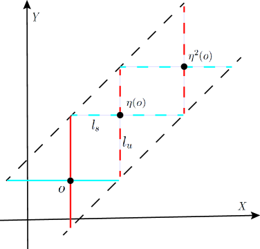
Figure 1. The skew ${\mathbb{R}}$-covered orbit space ${\mathcal{O}}$ and the map $\eta$

There is a very special continuous fixed point free map $\eta:{\mathcal{O}}\to{\mathcal{O}}$, which is called the half-step up map by Barthelme and Mann [BM]. $\eta$ is defined as follows. Take a point $o\in{\mathcal{O}}$, let $l_{s}$ be a stable leaf that is the upper boundary of the strip consisting of the unstable leaves through $o$, and $l_{u}$ be a unstable leaf that is the upper boundary of the strip consisting of the stable leaves through $o$. We define by $\eta(o)$ the intersection point of $l_{s}$ and $l_{u}$. This map exchanges stable leaves and unstable leaves, so $\tau=\eta^{2}$ preserves the stable leaves (resp. unstable leaves). $\eta$ can induce an orbit equivalence between $\phi_{t}$ and $\phi_{-t}$ that is homotopic to $id$ on $M$. For simplicity, we still call the orbit equivalence by $\eta$. Then $\eta^{2}$ is a self-orbit equivalence of $\phi_{t}$ that is homotopic to $id$ on $M$.

Remark 2.1.

If $M$ is a closed hyperbolic $3$-manifold, then each of $\eta$ and $\eta^{2}$ is isotopic to $id$ on $M$. This is a direct consequence of a classical result due to Gabai, Meyerhoff and N. Thurston [GMT], which says that when $M$ and $N$ are two closed hyperbolic $3$-manifolds and $f,g:M\to N$ are two homotopic homeomorphisms, then $f$ is isotopic to $g$.

Moreover, $\eta$ is important to describe the homotopy class of the periodic orbits of $\phi_{t}$:

Proposition 2.2 (Barbot [Ba], Fenley [Fen]).

Let $\phi_{t}$ be a skew ${\mathbb{R}}$-covered Anosov flow on a closed orientable $3$-manifold, and $\alpha$ be a periodic orbit of $\phi_{t}$. Then all the orbits freely homotopic to a periodic orbit $\alpha$ are given by $\{\eta^{2k}(\alpha),k\in{\mathbb{Z}}\}$, and all the orbits freely homotopic to the inverse of $\alpha$ are given by $\{\eta^{2k+1}(\alpha),k\in{\mathbb{Z}}\}$. Moreover, if $M$ is a hyperbolic $3$-manifold, every two periodic orbits $\eta^{2k_{1}}(\alpha)$ and $\eta^{2k_{2}}(\alpha)$ ($k_{1}\neq k_{2}$) are different, and therefore there are infinitely many periodic orbits that are homotopic to $\alpha$.

Notice that in this case, we can replace free homotopy by isotopy by the following theorem due to Barthelme and Fenley [BF0].

Theorem 2.3.

Let $\phi_{t}$ be a skew ${\mathbb{R}}$-covered Anosov flow on a closed orientable $3$-manifold. If two periodic orbits of $\phi_{t}$ are freely homotopic, then in fact they are isotopic.

In the proof of Theorem 1.1, we also need the following result due to Barthelme and Gogolev [BG].

Theorem 2.4.

Let $\phi_{t}$ be a skew ${\mathbb{R}}$-covered Anosov flow on a closed orientable $3$-manifold $M$, and $h$ be a self orbit equivalence of $\phi_{t}$ that is isotopic to $id$ on $M$. Then there exist an integer $k$ such that $h\circ\eta^{-2k}$ preserves every orbit of $\phi_{t}$. Moreover, if $M$ is a hyperbolic $3$-manifold, $k$ above is unique.

3. A representation of $Mod^{+}(N)$

Firstly, we define a homeomorphism $g_{1}:W\to W$ by $g_{1}((x,y),t)=((x_{1},y_{1}),1-t)$ where $\left(\begin{array}[]{ccc}x_{1}\\ y_{1}\end{array}\right)=B_{1}\left(\begin{array}[]{ccc}x\\ y\end{array}\right)$ and $B_{1}=\left(\begin{array}[]{cc}0&1\\ -1&0\\ \end{array}\right)$. $g_{1}$ is well-defined that is essentially due to the fact that $B_{1}AB_{1}^{-1}=A^{-1}$. It is easy to check that $g_{1}$ is an orbit equivalence between the Anosov flows $Y_{t}$ and $Y_{-t}$ on $W$. Define $g_{2}:=(g_{1})^{2}:W\to W$. By an easy computation, one can get that $g_{2}((x,y),t)=((x_{2},y_{2}),t)$ where $\left(\begin{array}[]{ccc}x_{2}\\ y_{2}\end{array}\right)=B_{2}\left(\begin{array}[]{ccc}x\\ y\end{array}\right)$ and $B_{2}=B_{1}^{2}$. Moreover, $g_{2}$ is a self orbit equivalence of $Y_{t}$. Similarly define $g_{3}:=(g_{1})^{3}$, and one can get that $g_{3}((x,y),t)=((x_{3},y_{3}),1-t)$ where $\left(\begin{array}[]{ccc}x_{3}\\ y_{3}\end{array}\right)=B_{3}\left(\begin{array}[]{ccc}x\\ y\end{array}\right)$ and $B_{3}=B_{1}^{3}$. Moreover, similar to the case for $g_{1}$, $g_{3}$ is also an orbit equivalence between the Anosov flows $Y_{t}$ and $Y_{-t}$. $g_{0}=g_{1}^{4}$ is the identity map on $W$.

Lemma 3.1.

$\{[g_{0}],[g_{1}],[g_{2}],[g_{3}]\}$ is a subgroup of $Mod^{+}(W)$ that is isomorphic to ${\mathbb{Z}}_{4}$. Here $[g_{i}]$ ($i=0,1,2,3$) represents the isotopy class of $g_{i}$.

Proof.

It only needs to prove that each of $g_{1}$, $g_{2}$ and $g_{3}$ is not isotopic to $g_{0}=id$. Notice that $\omega$ can represent a free element of $H_{1}(W)$ since $\omega$ intersects to a fiber torus once. Then $g_{1}(\omega)=-\omega$ and $\omega$ are not isotopic in $W$, therefore $g_{1}$ is not isotopic to $g_{0}=id$. For the same reason, one can get that $g_{3}$ is not isotopic to $g_{0}=id$. $\{(\frac{1}{4},0),(\frac{1}{2},\frac{1}{4}),(\frac{1}{4},\frac{3}{4})\}$ and $\{(\frac{3}{4},0),(\frac{1}{2},\frac{3}{4}),(\frac{3}{4},\frac{1}{4})\}$ are two periodic orbits of $A$ which correspond to two different periodic orbits $\beta_{1}$ and $\beta_{2}$ of $Y_{t}$. Since $\left(\begin{array}[]{ccc}\frac{3}{4}\\ 0\end{array}\right)=B_{2}\left(\begin{array}[]{ccc}\frac{1}{4}\\ 0\end{array}\right)$ on ${\mathbb{T}}^{2}$, therefore, $g_{2}(\beta_{1})=\beta_{2}$. Notice that $\beta_{1}$ and $\beta_{2}$ are not freely homotopic due to Nielsen fixed point theory (see, e.g. [Ji]), therefore, $g_{2}$ is not isotopic to $g_{0}=id$. ∎

Blow up $O\in{\mathbb{T}}^{2}$ to a circle $S_{o}^{1}$ such that a point $x\in S_{o}^{1}$ corresponds to a vector $\vec{v}\in T_{o}^{1}({\mathbb{T}}^{2})$. And ${\mathbb{T}}^{2}$ is blowed up to a punctured torus $T_{0}$ such that,

1. $\partial T_{0}=S_{o}^{1}$;

2. every point $x\in S_{o}^{1}$ is the starting point of the ray associted to the ray $l_{x}$ in ${\mathbb{T}}^{2}$ that starts at $O$ and is parallel to $\vec{v}$, where $\vec{v}\in T_{o}^{1}({\mathbb{T}}^{2})$ and corresponds to $x$.

Naturally we can identify ${\mathbb{T}}^{2}\setminus\{O\}$ with $T_{0}\setminus S_{o}^{1}$ by a homeomorphism $\phi:{\mathbb{T}}^{2}\setminus\{O\}\to T_{0}\setminus S_{o}^{1}$. The self homeomorphism $\phi A\phi^{-1}$ on $T_{0}\setminus S_{o}^{1}$ can be extended to a homeomorphism $\overline{A}:T_{0}\to T_{0}$ as follows. Recall that every point $x\in S_{o}^{1}$ corresponds to a ray $l_{x}$ in ${\mathbb{T}}^{2}$ that starts at $O$. $A$ maps $l_{x}$ to another ray $l$ starting at $O$. Let $y$ be the end of $\phi(l\setminus\{O\})$. Then $\overline{A}(x):=y$. One can automatically check that $\overline{A}$ is a homeomorphism on $T_{0}$. For every $i\in\{1,2,3\}$, the self homeomorphism $\phi B_{i}\phi^{-1}$ on $T_{0}\setminus S_{o}^{1}$ can be similarly extended to a homeomorphism $\overline{B_{i}}:T_{0}\to T_{0}$.

We can identify $N$ with $Map(T_{0},\overline{A})$ where $Map(T_{0},\overline{A})$ is the standard mapping torus of $\overline{A}$ on $T_{0}$. Take an oriented circle $l\subset\partial N$ that is the boundary of some $T_{0}\times\{t_{0}\}$ in $N$. Take another oriented circle $m\subset\partial N$ that intersects each circle $m_{t}=\partial T_{0}\times\{t\}$ ($t\in[0,1]$) at one point $q_{t}$ that is associated to a stable separatry of $A$ at $O$.

Notice that $B_{1}AB_{1}^{-1}=A^{-1}$ and the fact that $\overline{B}_{1}$ and $\overline{A}$ are the continuous extension of $\phi B_{1}\phi^{-1}$ and $\phi A\phi^{-1}$ respectively, then we have that $\overline{B}_{1}\overline{A}\overline{B}_{1}^{-1}=\overline{A}^{-1}$. Define a self homeomorphism $h_{1}$ on $N$ by $h_{1}(p,t):=(\overline{B}_{1}(p),1-t)$. $h_{1}$ is well-defined since $\overline{B}_{1}\overline{A}\overline{B}_{1}^{-1}=\overline{A}^{-1}$. Similarly, one can define a homeomorphism $h_{3}(p,t):=(\overline{B_{3}}(p),1-t)$ on $N$ and a homeomorphism $h_{2}(p,t):=(\overline{B_{2}}(p),t)$ on $N$. We define $h_{0}=id\mid_{N}$.

Proposition 3.2.

$Mod^{+}(N)=\{[h_{0}],[h_{1}],[h_{2}],[h_{3}]\}$ that is isomorphic to ${\mathbb{Z}}_{4}$. Here $[h_{i}]$ ($i=0,1,2,3$) represents the isotopy class of $h_{i}$.

Proof.

Due to their definitions, $h_{i}=\Phi g_{i}\Phi^{-1}$ on $N\setminus\partial N$ where $\Phi:W\setminus\omega\to N\setminus\partial N$ is defined by $\Phi(p,t):=(\phi(p),t)$. Recall that $(g_{i})^{n}=g_{ni}$ ($mod~{}4$), $g_{4k}=g_{0}=id$ and $h_{i}$ on $N$ is a continuous extension of $\Phi g_{i}\Phi^{-1}$ on $N\setminus\partial N$. Then we have that $(h_{i})^{n}=h_{ni}$ ($mod~{}4$) and $h_{4k}=h_{0}=id$. Since $[g_{i}]\in Mod^{+}(W)$, therefore, $[h_{i}]\in Mod^{+}(N)$. Notice that $Mod(N)\cong D_{4}$ and $Mod^{+}(N)\cong{\mathbb{Z}}_{4}$ (see, for instance [Mar]) where $D_{4}$ is the dihedral group that is the symmetry group of the square. So to complete the proof of this proposition, we are left to show that each of $h_{1}$, $h_{2}$ and $h_{3}$ is not isotopic to $h_{0}=id_{N}$. This essentially is the same to the proof that $g_{i}$ ($i=1,2,3$) is not isotopic to $g_{0}=id$ on $W$. Let us explain in detail.

Due to its definition, $h_{1}$ maps $m$ to $-m$. Further notice that $m$ intersects the once-punctured torus $T_{0}\times\{t_{0}\}$ once, then by using intersection number, one can easily prove that $h_{1}$ is not isotopic to $h_{0}=id_{N}$. Similarly we have that $h_{3}$ is not isotopic to $h_{0}=id_{N}$. In the proof of Lemma 3.1, we know that there are two disjoint oriented knots $\beta_{1}$ and $\beta_{2}$ in $W$ such that,

1. each of them is disjoint with $\omega$;

2. $g_{2}(\beta_{1})=\beta_{2}$

3. $\beta_{1}$ and $\beta_{2}$ are not freely homotopic in $W$.

Let $\beta_{1}^{\prime}=\Phi(\beta_{1})$ and $\beta_{2}^{\prime}=\Phi(\beta_{2})$ that are two disjoint oriented knots in $N$. It is easy to check that $\Phi:(W\setminus\omega,\beta_{1},\beta_{2})=(N\setminus\partial N,\beta_{1}^{\prime},\beta_{2}^{\prime})$. Notice that $\beta_{1}$ and $\beta_{2}$ are not freely homotopic in $W$, so $\beta_{1}$ and $\beta_{2}$ are not freely homotopic in $W\setminus\omega$ and therefore $\beta_{1}^{\prime}$ and $\beta_{2}^{\prime}$ are not freely homotopic in $N\setminus\partial N$. Hence $\beta_{1}^{\prime}$ and $\beta_{2}^{\prime}$ are not freely homotopic in $N$. Further observe that $h_{2}(\beta_{1}^{\prime})=\beta_{2}^{\prime}$ since $g_{2}(\beta_{1})=\beta_{2}$ and $h_{2}=\phi g_{2}\phi^{-1}$ in $N\setminus\partial N$. Then $\beta_{1}^{\prime}$ and $h_{2}(\beta_{1}^{\prime})$ are not freely homotopic in $N$, therefore $h_{2}$ is not isotopic to $h_{0}=id_{N}$. The proposition is proved. ∎

4. The homeomorphisms $f_{i}$ and $f_{i}^{\prime}$ on $M_{k}$

$\Phi:W\setminus\omega\to N\setminus\partial N$ maps the flow $Y_{t}$ on $W\setminus\omega$ to a flow $\Phi(Y_{t})$ on $N\setminus\partial N$. Then we can get the Anosov flow $X_{t}$ on $M_{k}$ from $Y_{t}$ through a DFG surgery. For our purpose, here we just introduce this procedure in Fried’s way ([Fr]). Due to Fried [Fr], $\Phi(Y_{t})$ can be continuously extended to a continuous flow $Z_{t}$ on $N$ such that $Z_{t}\mid_{\partial N}$ is a nonsingular Morse-Smale flow with $4$ periodic orbits with alternating orientations. (see Figure 2) Take a circle bundle $E$ on $\partial N$ such that each circle fiber $e$ is transverse to the flowlines of $Z_{t}\mid_{\partial N}$ and is isotopic to $l+km$ in $\partial N$. Here $m$ is a meridian circle of the figure-eight knot exterior $N$ and $l$ is a longitute circle of $N$ that is homology vanishing. We remark that up to isotopy, each of $m$ and $l$ is unique. By pinching every circle fiber $e$ to a point $x_{e}$, we blow down $N$ to the manifold $M_{k}$ by the pinching map $\pi:N\to M_{k}$. Moreover, the flow $Z_{t}$ on $N$ is blowed down to the Anosov flow $X_{t}$ on $M_{k}$. See Figure 2.

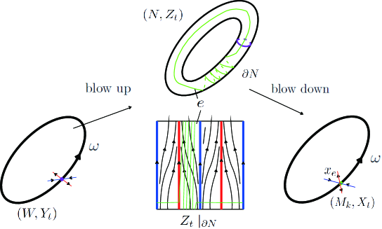
Figure 2. Fried surgery in the case $k=5$

Since $g_{2}$ is a self orbit equivalence of $Y_{t}$, then $\Phi g_{2}\Phi^{-1}$ is a self orbit equivalence of $\Phi(Y_{t})$ on $W\setminus\omega$. Moreover, since $Z_{t}$ is a continuous extension of $\Phi(Y_{t})$, then as a continuous extension of $\Phi g_{2}\Phi^{-1}$ on $N$, $h_{2}$ is is a self orbit equivalence of $Z_{t}$ on $N$. Further notice that up to isotopy, $h_{2}:m\to m$ and $h_{2}:l\to l$. Then up to isotopy, $h_{2}$ preserves the circle fibration structure $E$ on $\partial N$. Then, after composing a self orbit equivalence preserving every orbit if necessary, we can assume that $h_{2}$ preserves $E$. Then $h_{2}$ naturally induces a self orbit equivalence $f_{2}$ of $X_{t}$ on $M_{k}$ such that $\pi h_{2}=f_{2}\pi$. Notice that $g_{i}$ ($i=1,3$) is an orbit equivalence between $Y_{t}$ and $Y_{-t}$, and $h_{i}:m\to-m$ and $h_{i}:l\to-l$. Then similarly, after composing a self orbit equivalence preserving every orbit if necessary, $h_{i}$ naturally induces an orbit equivalence $f_{i}$ between $X_{t}$ and $X_{-t}$ on $M_{k}$ such that $\pi h_{i}=f_{i}\pi$. $h_{0}=id\mid_{N}$ naturally induces $f_{0}=id$ on $M_{k}$. We can conclude the above discussion to the following lemma.

Lemma 4.1.

For every $i\in\{0,1,2,3\}$, after composing a self orbit equivalence preserving every orbit of $Z_{t}$ if necessary, the self homeomorphism $h_{i}$ on $N$ induces a self homeomorphism $f_{i}$ on $M_{k}$ such that $\pi h_{i}=f_{i}\pi$. Moreover,

1. if $i=0$ or $i=2$, $f_{i}$ is a self orbit equivalence of $X_{t}$ on $M_{k}$;

2. if $i=1$ or $i=3$, $f_{i}$ is an orbit equivalence between $X_{t}$ and $X_{-t}$ on $M_{k}$.

Let $V$ be a solid torus tubular neighborhood of $\omega$, then the closure of $M_{k}\setminus V$ is homeomorphic to $N$. For simplicity, we still call it $N$. Then we can think that $M_{k}=V\cup_{\psi_{k}}N$ where $\psi_{k}:\partial V\to\partial N$ is the corresponding gluing map such that up to isotopy, $\psi_{k}(m_{v})=l+km$. Here $m_{v}$ is a meridian circle of the solid torus $V$. Now we extend the homeomorphism $h_{i}$ ($i=0,1,2,3$) on $N$ to $f_{i}^{\prime}$ on $M_{k}$. First, $h_{0}=id\mid_{N}$, it can be naturally extended to $f_{0}^{\prime}=f_{0}=id$ on $M_{k}$. In the other three cases, since up to isotopy $h_{i}$ maps $m$ to $m$ or $-m$, there is no obstruction to extend $h_{i}$ to a homeomorphism $f_{i}^{\prime}$ on $M_{k}$ such that $f_{i}^{\prime}$ maps $\omega$ to itself. Moreover, it is easy to observe that $f_{i}^{\prime}$ and $f_{i}$ are isotopic.

5. Proof of the main theorem

The following lemma was firstly used in the study of Anosov flows by Bowden and Mann ([BM]). Both of the statement and the proof essentially follow [BM].

Lemma 5.1.

If $|k|\gg 0$, then for every self homeomorphism $f$ on $M_{k}$, up to isotopy, $f(\omega)=\omega$.

Proof.

Due to [Thu], up to isotopy, $\omega$ is the unique shortest closed geodesic in the hyperbolic three manifold $M_{k}$. Due to Mostow rigidity, up to isotopy, $f$ is an isometry on $M_{k}$, and therefore $f(\omega)$ is a shortest closed geodeic in $M_{k}$. But $\omega$ is the unique shortest closed geodesic in $M_{k}$, hence up to isotopy, $f(\omega)=\omega$. ∎

Lemma 5.2.

If $|k|\gg 0$, we endow an (in fact, any) orientation on $M_{k}$. Then for every self homeomorphism $f$ on $M_{k}$, up to isotopy, $f$ preserves the orientation on $M_{k}$.

Proof.

Due to Lemma 5.1, up to isotopy, we can assume that $f(\omega)=\omega$. Recall that $M_{k}=V\cup_{\psi_{k}}N$. Here $V$ is a solid torus with a core $\omega$, $N$ is the figure-eight knot exterior (see Section 3) and $\psi_{k}:\partial V\to\partial N$ is the corresponding gluing homeomorphism. Since $f(\omega)=\omega$, up to isotopy, we can assume $f(V)=V$ and $f(N)=N$. Further recall that up to isotopy, $\psi_{k}(m_{v})=l+km$ where $m_{v}$ is an oriented merdian circle of $V$ and $m$ and $l$ are the standard oriented meridian circle and oriented longitute circle in $\partial N$.

We assume by contradiction that $f$ is not orientation preserving, then $f\mid_{N}$ is also not orientation preserving. Since up to isotopy, as the meridian of the figure-eight knot exterior and as the unique longitute which is homology vanishing, each of $m$ and $l$ is unique. This means that in this case, up to isotopy, either $f(l)=-l$ and $f(m)=m$, or $f(l)=l$ and $f(m)=-m$. Further since up to isotopy, $\psi_{k}(m_{v})=l+km$ on $\partial N$, then $f(\psi_{k}(m_{v}))$ is isotopic to $\pm(l-km)$ on $\partial N$. This is impossible since $f(\psi_{k}(m_{v}))$ must bounds a disk in $V$ in $M_{k}=V\cup_{\psi_{k}}N$, but such a circle must isotopes to either $l+km$ or $-l-km$ in $\partial N$. The proof of the lemma is complete. ∎

Lemma 5.3.

Let $f$ be a self homeomorphism on $M_{k}$, then $f$ is isotopic to one of $f_{0}=id$, $f_{1}$, $f_{2}$ and $f_{3}$.

Proof.

By Lemma 5.1 and Lemma 5.2, $f$ is oriention-preserving and up to isotopy, we can assume that $f(V,\omega)=(V,\omega)$ and $f(N)=N$. Then by Proposition 3.2, $f\mid_{N}$ is isotopic to some $h_{i}=f_{i}^{\prime}\mid_{N}$. Define $g:=(f_{i}^{\prime})^{-1}\circ f$ that is a homeomorphism on $M_{k}$ such that $g(V,\omega)=(V,\omega)$, $g(N)=N$ and $g\mid_{N}$ is isotopic to $f_{0}\mid_{N}=id_{N}$. Since $f_{i}$ and $f_{i}^{\prime}$ are isotopic (see Section 4), to complete the proof of this lemma, we are left to show that $g$ is isotopic to $f_{0}=id$ on $M_{k}$. From now on, we focus on showing this.

Since $g:N\to N$ is isotopic to $f_{0}\mid_{N}=id_{N}$, then up to isotopy, we can assume $g(m)=m$ and $g(l)=l$. This fact permits us to assume that $g\mid_{V}=id_{V}$ up to isotopy. Let $V_{1}$ be a compact tubular neighborhood of $\omega$ in the interior of $V$. Let $U$ be the cloure of $V-V_{1}$ that can be paramerized by ${\mathbb{T}}^{2}\times[0,1]$ such that ${\mathbb{T}}^{2}\times\{0\}$ and ${\mathbb{T}}^{2}\times\{1\}$ correspond to $\partial N=\partial V$ and $\partial V_{1}$ respectively.

Let $F_{t}:N\to N$ ($t\in[0,1]$) be an isotopy such that $F_{0}=id_{N}$ and $F_{1}=g\mid_{N}$. $F_{t}$ can be extended to an isotopy $F_{t}^{\prime}$ on $M_{k}$ such that

1. $F_{t}^{\prime}=F_{t}$ on $N$,

2. $F_{t}^{\prime}(x,s)=(F_{t(1-s)}(x),s)$ on $U$ where $x\in{\mathbb{T}}^{2}$ and $s\in[0,1]$,

3. $F_{t}^{\prime}=id$ on $V_{1}$.

One can automatically check that $F_{t}^{\prime}$ is an isotopy between $F_{0}^{\prime}=f_{0}$ and $F_{1}^{\prime}$ on $M_{k}$. Furthermore, it is easy to check that $F_{1}^{\prime}$ and $g$ are isotopic on $M_{k}$. Therefore, $g$ is isotopic to $f_{0}=id$ on $M_{k}$. The proof of the lemma is complete. ∎

Lemma 5.4.

$f_{0}$ and $f_{2}$ are two self orbit equivalences of $X_{t}$, and $F_{1}:=\eta\circ f_{1}$ and $F_{3}:=\eta\circ f_{3}$ are two self orbit equivalences of $X_{t}$. Moreover, $F_{1}$ is isotopic to $f_{1}$ and $F_{3}$ is isotopic to $f_{3}$.

Proof.

By Lemma 4.1, each of $f_{0}$ and $f_{2}$ is a self orbit equivalence of $X_{t}$, and each of $f_{1}$ and $f_{3}$ is a self orbit equivalence between $X_{t}$ and $X_{-t}$. By Section 2, $\eta$ is also an orbit equivalence between $X_{t}$ and $X_{-t}$. Therefore, each of $F_{1}=\eta\circ f_{1}$ and $F_{3}=\eta\circ f_{3}$ is a self orbit equivalence of $X_{t}$. Morever, notice that $\eta$ is isotopic to $f_{0}=id$ on $M_{k}$ (see Remark 2.1), therefore $F_{1}$ is isotopic to $f_{1}$ and $F_{3}$ is isotopic to $f_{3}$. ∎

Lemma 5.5.

$f_{2}$ is not isotopic to $f_{0}=id$.

Proof.

Assume by contradiction that $f_{2}$ is isotopic to $f_{0}=id$, then by Theorem 2.4, there is a unique $k\in{\mathbb{Z}}$ such that $h=f_{2}\circ\eta^{-2k}$ is a self orbit equivalence of $X_{t}$ such that $h$ preserves each orbit of $X_{t}$. Moreover, by Proposition 2.2, for every $i\in{\mathbb{Z}}\setminus\{0\}$, $h\circ\eta^{2i}$ does not preserve each periodic orbit of $X_{t}$. Notice that $f_{2}(\omega)=\omega$, therefore $k=0$ and $h=f_{2}$. This means that $f_{2}$ must preserve each periodic orbit of $X_{t}$.

Similar to the proof of Lemma 3.1, $\{(\frac{1}{4},0),(\frac{1}{2},\frac{1}{4}),(\frac{1}{4},\frac{3}{4})\}$ and $\{(\frac{3}{4},0),$ $(\frac{1}{2},\frac{3}{4}),(\frac{3}{4},\frac{1}{4})\}$ are two periodic orbits of $A$ which correspond to two different periodic orbits $\beta_{1}$ and $\beta_{2}$ of $X_{t}$. Since $\left(\begin{array}[]{ccc}\frac{3}{4}\\ 0\end{array}\right)=B_{2}\left(\begin{array}[]{ccc}\frac{1}{4}\\ 0\end{array}\right)$ on ${\mathbb{T}}^{2}$, therefore $f_{2}(\beta_{1})=\beta_{2}$. This conflicts to the fact that $f_{2}$ must preserve each periodic orbit of $X_{t}$. Then, the assumption is not correct and therefore $f_{2}$ is not isotopic to $f_{0}=id$. ∎

The result of the following lemma should be classical, but we have not found a related reference, so we give a proof here.

Lemma 5.6.

Let $f$ be a homeomorphism on the solid torus $V$ such that $f\mid_{\partial V}=id\mid_{\partial V}$, then $f$ is isotopic to $id$ on $V$ relative to $\partial V$.

Proof.

Let $m$ be a meridian circle in $\partial V$ that bounds a meridian disk $D$ in $V$. By an isotopy relative to $\partial V$ if necessary, we can assume that the interior of $f(D)$ intersects with $D$ at finitely many pairwise simple closed curves. Notice that $V$ is an irreducible $3$-manifold, then by a standard ‘inner most disk’ combinatorial topology trick, by a further isotopy relative to $\partial V$ if necessary, we can assume that the interior of $f(D)$ is disjoint with $D$. Therefore $S=f(D)\cup D$ is a two sphere in $V$ such that $S\cap V=m$ and $S$ bounds a three ball in $V$. Then after an isotopy relative to $\partial V$, we can assume that $f(D)=D$.

Since $f\mid_{\partial D}=id_{\partial D}$, then by using two dimentional Alexander trick, $f\mid_{\partial D}$ is isotopic to $id_{\partial D}$ relative to $\partial D$ by an isototy $h_{t}$ on $D$ such that $h_{0}=id_{D}$ and $h_{1}=(f\mid_{D})^{-1}$. Find a small compact neighborhood $U(D)$ of $D$ such that $U(D)\cap\partial V=m$ and $U(D)$ can be parameterized by $D\times[-1,1]$ modular $(x,s_{1})=(x,s_{2})$ ($s_{1},s_{2}\in[-1,1]$). See Figure 3 as an illustration. Define an isotopy $H_{t}$ on $V$ by $H_{t}(y)=y$ if $y\notin U(D)$ and $H_{t}(x,s)=(h_{(1-|s|)t}(x),s)$ ($x\in D$ and $s\in[-1,1]$). Define $G_{t}:=H_{t}\circ f$. Then one can automatically check that $G_{0}=f$ and $(G_{1})\mid_{\partial V\cup D}=id_{\partial V\cup D}$, and $G_{0}=f$ and $G_{1}$ are isotopic relative to $\partial V$. Then by using three dimentional Alexander trick on the three ball which is the path closure of $V\setminus(\partial V\cup D)$, we have that $G_{1}$ is isotopic to $id_{V}$ relative to $\partial V$. Therefore, $f=G_{0}$ is isotopic to $id$ on $V$ relative to $\partial V$. ∎

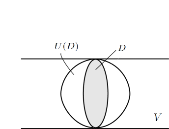
Figure 3. Some notations in the proof of Lemma 5.6

The conclusion in the following lemma is elementary but useful.

Lemma 5.7.

Let $\phi_{0}$ and $\phi_{1}$ be two homeomorphisms on $M_{k}$ such that

1. $\phi_{i}(N)=N$ and $\phi_{i}(V)=V$ for $i=1,2$;

2. $(\phi_{0})\mid_{N}$ and $(\phi_{1})\mid_{N}$ are isotopic, and $(\phi_{0})\mid_{V}$ and $(\phi_{1})\mid_{V}$ are isotopic.

Then $\phi_{0}$ and $\phi_{1}$ are isotopic on $M_{k}$.

Proof.

Let $F_{t}$ ($t\in[0,1]$) be an isotopy on $N$ such that $F_{0}=(\phi_{0})\mid_{N}$ and $F_{1}=(\phi_{1})\mid_{N}$. Let $G_{t}$ ($t\in[0,1]$) be an isotopy on $V$ such that $G_{0}=(\phi_{0})\mid_{V}$ and $G_{1}=(\phi_{1})\mid_{V}$. Obviously, for $i=0$ or $i=1$, $(\phi_{i})\mid_{\partial N}=\psi_{k}(\phi_{i})\mid_{\partial V}(\psi_{k})^{-1}$. Define $h_{t}:=(\psi_{k})^{-1}F_{t}\psi_{k}(G_{t})^{-1}:\partial V\to\partial V$. It can be automatically checked that $h_{t}$ is an isotopy on $\partial V$ such that $h_{0}=h_{1}=id\mid_{\partial V}$.

Now we paramterize a small closed collar neighborhood $U(\partial V)$ of $\partial V$ in $V$ by $\partial V\times[0,1]$ such that $\partial V\times\{1\}$ identifies to $\partial V$. Let $V_{0}$ be the closure of $V\setminus U(\partial V)$. Define an isotopy $H_{t}$ on $V$ by $H_{t}=id_{V_{0}}$ on $V_{0}$ and $H_{t}(s,x)=(s,h_{st}(x))$ ($s,t\in[0,1]$) on $U(\partial V)$. It is easy to check that $H_{0}=id$ on $V$ and $(H_{1})\mid_{\partial V}=id\mid_{\partial V}$.

Then $H_{t}G_{t}$ is an isotopy on $V$ such that $(H_{t}G_{t})\mid_{\partial V}=h_{t}G_{t}=(\psi_{k})^{-1}F_{t}\psi_{k}$ and $H_{0}G_{0}=G_{0}=(\phi_{0})\mid_{V}$ and $(H_{1}G_{1})_{\partial V}=(G_{1})_{V}=(\phi_{1})_{V}$. Then we can define an isotopy $K_{t}$ on $M_{k}$ by $K_{t}=F_{t}$ on $N$ and $K_{t}=H_{t}G_{t}$ on $V$ between $\phi_{0}$ and $\phi_{1}^{\prime}$, where $\phi_{1}^{\prime}=\phi_{1}$ on $N$ and $\phi_{1}^{\prime}=H_{1}G_{1}$ on $V$.

Define a homeomorphism $g:=\phi_{1}^{-1}\phi_{1}^{\prime}$ on $M_{k}$. Then $g\mid_{N}=id_{N}$, and by Lemma 5.6, it is easy to get that $g$ is isotopic to $id$ on $M_{k}$. Equivalently, $\phi_{1}^{\prime}$ is isotopic to $\phi_{1}$. Thereroe, $\phi_{0}$ and $\phi_{1}$ are isotopic on $M_{k}$. ∎

Lemma 5.8.

$(f_{1})^{2}=f_{1}\circ f_{1}$ is isotopic to $f_{2}$, $(f_{1})^{3}$ is isotopic to $f_{3}$ and $(f_{2})^{2}$ is isotopic to $f_{0}=id$.

Proof.

By the final part of Section 4, we know that $f_{i}$ ($i=0,1,2,3$) is isotopic to $f_{i}^{\prime}$ on $M_{k}$. Therefore we only need to prove the lemma through replacing $f_{i}$ by $f_{i}^{\prime}$. Since $f_{i}^{\prime}$ is an extension of $h_{i}$ on $N$, by Proposition 3.2, we know that $(f_{1}^{\prime})^{2}\mid_{N}$ is isotopic to $f_{2}^{\prime}\mid_{N}$, $(f_{1}^{\prime})^{3}\mid_{N}$ is isotopic to $f_{3}^{\prime}\mid_{N}$ and $(f_{2}^{\prime})^{2}\mid_{N}$ is isotopic to $f_{0}^{\prime}\mid_{N}=id_{N}$. Moreover, based on the fact that the isotopy class of a homeomorphism $g$ on $V$ is decided by the isotopy classes of $g(m)$ and $g(l)$ on $\partial V$, one can automatically check that $(f_{1}^{\prime})^{2}\mid_{V}$ is isotopic to $f_{2}^{\prime}\mid_{V}$, $(f_{1}^{\prime})^{3}\mid_{V}$ is isotopic to $f_{3}^{\prime}\mid_{V}$ and $(f_{2}^{\prime})^{2}\mid_{V}$ is isotopic to $f_{0}^{\prime}\mid_{V}=id_{V}$. Then, the conclusion of the lemma can be obtained from Lemma 5.7. ∎

Now we are prepared enough to prove the main theorem.

Proof of Theorem 1.1.

By Lemma 5.8, $f_{2}$ is isotopic to $(f_{1})^{2}$, $f_{3}$ is isotopic to $(f_{1})^{3}$ and $(f_{1})^{4}$ is isotopic to $f_{0}=id$. Therefore $f_{3}$ is isotopic to $(f_{1})^{-1}$. By Lemma 5.5, $f_{2}$ is not isotopic to $f_{0}=id$. Therefore each of $f_{1}$ and $f_{3}$ is not isotopic to $f_{0}=id$ since $f_{2}$ is isotopic to $(f_{1})^{2}$ and $f_{3}$ is isotopic to $(f_{1})^{-1}$. Further by Lemma 5.3, each self homeomorphism $f$ on $M_{k}$ is isotopic to some $(f_{1})^{i}$ ($i=0,1,2,3$). Then following the above discussions, one can easily get that $Mod(M_{k})=<[f_{1}]>\cong{\mathbb{Z}}_{4}$.

By Lemma 5.4, in each isotopy class of $f_{i}$ ($i=0,1,2,3$), there exists a self orbit equivalence of $X_{t}$ ($f_{i}$ if $i=0,2$ and $g_{i}$ if $i=1,3$) in this class. This means that every element in $Mod(M_{k})$ can be represented by a self orbit equivalence of $X_{t}$. The proof of Theorem 1.1 is complete. ∎

Bin Yu

School of Mathematical Sciences

Key Laboratory of Intelligent Computing and Applications (Tongji University), Ministry of Education

Tongji University, Shanghai 200092, CHINA

E-mail: binyu1980@gmail.com

References

- [Ano] Anosov, D. V. Geodesic flows on closed Riemannian manifolds of negative curvature. Trudy Mat. Inst. Steklov. 90 (1967).
- [Ba] Thierry Barbot. Caractérisation des flots d’Anosov en dimension 3 par leurs feuilletages faibles. Ergodic Theory Dynam. Systems 15 (1995), no. 2, 247-270.
- [Bart] Thomas Barthelme. School on contemporary dynamical systems: Anosov flows in dimension . 2017.
- [BF0] Thomas Barthelmé; Sergio Fenley. Knot theory of R-covered Anosov flows: homotopy versus isotopy of closed orbits. J. Topol. 7 (2014), no. 3, 677-696.
- [BaFe] Thomas Barthelmé; Sergio Fenley. Counting periodic orbits of Anosov flows in free homotopy classes. Comment. Math. Helv. 92 (2017), no. 4, 641-714.
- [BFP] Thomas Barthelmé, Sergio Fenley, Rafael Potrie Collapsed Anosov flows and self orbit equivalences. Arxiv:2008.06547.
- [BG] Thomas Barthelmé; Gogolev, Andrey. A note on self orbit equivalences of Anosov flows and bundles with fiberwise Anosov flows. Math. Res. Lett. 26 (2019), no.3, 711-728.
- [BM] Thomas Barthelmé, Kathryn Mann. Orbit equivalences of -covered Anosov flows and hyperbolic-like actions on the line. Arxiv: 2012.11811
- [BM] Bowden, J; Mann, K. stability of boundary actions and inequivalent Anosov flows. Ann. Sci. Éc. Norm. Supér. (4) 55 (2022), no. 4, 1003–1046.
- [Fen] Sergio, Fenley. Anosov flows in 3-manifolds. Ann. of Math. (2) 139 (1994), no. 1, 79-115.
- [FP1] Sergio Fenley, Rafael Potrie. Partial hyperbolicity and pseudo-Anosov dynamics. ArXiv:2102.02156
- [FP2] Sergio Fenley, Rafael Potrie. Accessibility and ergodicity for collapsed Anosov flows. ArXiv:2103.14630
- [Fr] Fried, D. Transitive Anosov flows and pseudo-Anosov maps. Topology 22 (1983), no. 3, 299-303.
- [GMT] Gabai, David; Meyerhoff, Robert; Thurston, Nathaniel. Homotopy hyperbolic 3-manifolds are hyperbolic. Ann. of Math. (2)157(2003), no.2, 335-431.
- [Go] Goodman, S. “Dehn surgery on Anosov flows” in Geometric Dynamics, Rio de Janeiro, 1981, Lecture Notes in Math. 1007, Springer, Berlin, 1983, 300–307.
- [Ji] B. Jiang, Lectures on Nielsen Fixed Point Theory, Contemporary Mathematics, vol.14, American Mathematical Society, Providence, 1983.
- [Mar] Martelli, B. An Introduction to Geometric Topology. CreateSpace Independent Publishing Platform. 2016.
- [Sha] Shannon, M. Dehn surgeries and smooth structures on 3-dimensional transitive Anosov flows. Thesis (Ph.D.)-University of Burgundy. 2020. 189 PP.
- [Thu] Thurston, Williams. The geometry and topology of 3-manifolds. 360 pages, Lecture notes, http://www.msri.org/publications/books/ gt3m.
- [Yu] Yu, Bin. Anosov flows on Dehn surgeries on the figure-eight knot. Duke Math. J.172(2023), no.11, 2195-2240.
Bin Yu