Learning Bayesian networks:
a copula approach for mixed-type data

Abstract

Estimating dependence relationships between variables is a crucial issue in many applied domains, such as medicine, social sciences and psychology. When several variables are entertained, these can be organized into a network which encodes their set of conditional dependence relations. Typically however, the underlying network structure is completely unknown or can be partially drawn only; accordingly it should be learned from the available data, a process known as structure learning. In addition, data arising from social and psychological studies are often of different types, as they can include categorical, discrete and continuous measurements. In this paper we develop a novel Bayesian methodology for structure learning of directed networks which applies to mixed data, i.e. possibly containing continuous, discrete, ordinal and binary variables simultaneously. Whenever available, our method can easily incorporate known dependence structures among variables represented by paths or edge directions that can be postulated in advance based on the specific problem under consideration. We evaluate the proposed method through extensive simulation studies, with appreciable performances in comparison with current state-of-the-art alternative methods. Finally, we apply our methodology to well-being data from a social survey promoted by the United Nations, and mental health data collected from a cohort of medical students.

Keywords: Bayesian inference; Directed acyclic graph; Markov chain Monte Carlo; Network psychometrics, Structural equation model.

1 Introduction

1.1 Background and motivation

Learning dependence relations between variables is a pervasive issue in many applied domains, such as biology, social sciences, and notably psychology (Briganti et al., 2022; Isvoranu et al., 2022). In the latter context, the recent field of network psychometrics considers a network-based approach to represent psychological constructs and understand directed interactions between behavioral, cognitive and biological factors, possibly allowing for causal interpretations (Borsboom et al., 2021). The 2022 Psychometrika special issue “Network Psychometrics in action” promoted the development of statistical methods for network modelling motivated by psychological problems, and collected several contributions to the field, covering both methodological and applied aspects (Marsman & Rhemtulla, 2022).

Early works in the network psychometrics area were conceived to support psychologists in providing insights on various psychological phenomena, such as those at the basis of psychopatology, and in particular the study of comorbidity and mental disorders (Borsboom, 2008; Cramer et al., 2010). Typical research questions thus relate to the identification of direct dependencies between manifest variables, differences in the underlying dependence structure across available groups of patients, or even to the design of clinical interventions based on an estimated network. Crucial to these purposes is the development of models that allow to infer a plausible network structure for the available data and to provide a coherent quantification of the uncertainty related to directed links, specific paths or the whole network structure. In this regard, methodologies that fully account for network uncertainty lead to parameter estimates that are more robust w.r.t. possible network-model misspecifications; see Haslbeck & Waldorp (2018), Epskamp et al. (2017) and Marsman et al. (2022) for recent contributions in this area inspired by psychological problems.

All of the issues introduced above have motivated the development of dedicated statistical methodologies, based both on a frequentist and on a Bayesian paradigm. In particular, probabilistic graphical models based on directed networks provide an effective tool to infer conditional dependence relations from the data (Cowell et al., 1999; Edwards, 2000). Additionally, Directed Acyclic Graphs (DAGs) offer a powerful framework for causal reasoning, even from observational, namely non-experimental, studies and specifically to quantify effects of hypothetical interventions on target variables w.r.t. outcome responses of interest; see Pearl (2000) for a general introduction on causal inference based on DAGs, Maathuis & Nandy (2016) for a review. The next section offers an overview of the main recent contributions to graphical modelling.

1.2 Literature review

From a statistical perspective, learning a network of dependencies from the data is a model selection problem also known as structure learning. Several related methodologies that can deal with Gaussian and categorical data separately have been proposed. Specifically, score-based methods implement score functions for network estimation, such as based on penalized maximum likelihood estimators (Meinshausen & Bühlmann, 2006; Friedman et al., 2008), or marginal likelihoods for methodologies following a Bayesian perspective (Heckerman et al., 1995; Chickering, 2002). Moreover, constraint-based methods implement conditional independence tests to learn the set of (in)dependence constraints characterizing the underlying DAG structure, as in the popular PC algorithm (Spirtes et al., 2000; Kalisch & Bühlmann, 2007). On the other hand, Bayesian methodologies adopt Markov chain Monte Carlo (MCMC) methods to approximate a posterior distribution over the space of network structures, or related features of interest; see for instance Castelletti et al. (2018) and Castelletti & Peluso (2021) for respectively Gaussian and categorical settings, Ni et al. (2022) for a recent overview of Bayesian methods for structure learning with applications to biological problems.

Mixed-type data, i.e. observations from variables of different parametric families, are very common in many contexts and expecially psychological studies, where ordinal, discrete and continuous measurements are simultaneously collected on subjects. A few methodologies for structure learning from mixed data have been proposed. Harris & Drton (2013) introduce the rank PC, an extension of the original PC algorithm to nonparanormal models, namely based on a semi-parametric latent Gaussian copula model, with purely continuous marginal distributions. Moreover, Cui et al. (2016) propose the Copula PC, an adaptation of the PC algorithm to a mixture of discrete and continuous data assumed to be drawn from a Gaussian copula model. Cui et al. (2018) extend the previous method to deal with data that are missing at random. Similar ideas, for the case of undirected graphs, are also considered by Müller & Czado (2019) and He et al. (2017). Still in the context of directed graphs, a more recent methodology for structure learning given both categorical and Gaussian data is proposed by Andrews et al. (2018). The authors introduce a mixed-variable polynomial score based on the notion of Conditional Gaussian (CG) distribution (Lauritzen & Wermuth, 1989), then extended to a highly scalable algorithm by Andrews et al. (2019). Conditional Gaussian distributions are also adopted for structure learning of undirected graphs by Lee & Hastie (2013) and Cheng et al. (2017) who implement penalized likelihoods and regression models with weighted lasso penalties respectively. In a Bayesian setting, Bhadra et al. (2018) propose a unified framework for both categorical and Gaussian data based on Gaussian scale mixtures.

One main difficulty in developing statistical models for general mixed-type data is related to the non-standard joint support of the available variables. Typically however, interest lies in estimating dependence parameters of the joint distribution, corresponding to a network structure or correlation-type measures, rather than parameters indexing the marginal distributions of the variables. In this context, copula models, which allow to model the two sets of parameters separately, can provide an effective solution for statistical inference of network models. In addition, semiparametric copula models lacks any parametric assumption on the marginal c.d.f.’s which are estimated through their empirical distributions (Hoff, 2007). Contributions to copula graphical modelling based on undirected graphs are provided by Dobra & Lenkoski (2011) and Mohammadi et al. (2017).

1.3 Contribution and structure of the paper

We propose a novel methodology for structure learning of networks which applies to mixed data, i.e. comprising continuous, categorical as well as discrete and ordinal measurements. Specifically, we consider a Gaussian copula model where the dependence parameter (covariance matrix) reflects the conditional independencies imposed by a directed acyclic graph, leading to our Gaussian copula DAG model. We consider a Bayesian framework and proceed by assigning suitable prior distributions to DAG structures and DAG-dependent parameters. Inference is carried out by implementing an MCMC scheme which approximates the posterior distribution over network structures and covariance matrices. The main contributions of the proposed method can be summarized as follows: i) we introduce a Bayesian framework for the analysis of complex dependence relations in multivariate settings characterized by mixed data; ii) we provide a coherent quantification of the uncertainty around the estimated network or features of interest such as directed links, and a full posterior distribution of the underlying dependence parameter (correlation matrix), possibly summarized by Bayesian Model Averaging (BMA) estimates; iii) our model allows to incorporate prior knowledge of the underlying network in terms of a partial ordering of the variables or edge orientations that are known in advance, thus improving DAG identification and enhancing causal inference.

The rest of the paper is organized as follows. In Section 2 we introduce Gaussian graphical models based on DAGs and the copula DAG model that we adopt for the analysis of mixed data. Section 3 completes our Bayesian model formulation by assigning prior distributions to DAG structures and DAG-model parameters. We implement in Section 4 an MCMC scheme which approximates the posterior distribution of DAGs and parameters. Our method is evaluated through extensive simulation experiments in Section 5. Section 6 is devoted to empirical studies, including the analysis of well-being data from a social survey promoted by the United Nations and mental health data collected from a cohort of medical students. In Section 7 we finally provide a discussion together with possible extensions of the proposed method to heterogeneous settings and latent trait models. Additional simulation results, comparisons with alternative methods and examples of MCMC diagnostics of convergence are included in the Appendix.

2 Model specification

2.1 Directed acyclic graphs

A Directed Acyclic Graph (DAG) is a pair $\mathcal{D}=(V,E)$ consisting of a set of vertices (or nodes) $V=\{1,\dots,q\}$ and a set of directed edges $E\subseteq V\times V$. For any two nodes $u,v\in V$, we denote an edge from $u$ to $v$ as $(u,v)$ or $u\rightarrow v$ indifferently; also, the set $E$ is such that if $(u,v)\in E$ then $(v,u)\notin E$. A sequence of nodes $(v_{1},v_{2},\dots,,v_{k})$ is a path if there exists $v_{1}\rightarrow v_{2}\rightarrow\cdots\rightarrow v_{k}$ in $\mathcal{D}$. We assume that $\mathcal{D}$ does not contain cycles, that is paths such that $v_{1}\equiv v_{k}$. For a given node $v\in V$ we let $\mathrm{pa}_{\mathcal{D}}(v)$ be the set of parents of $v$ in $\mathcal{D}$, i.e. the set of all nodes $u$ such that $(u,v)\in E$. Moreover, we say that $u$ is a descendant of $v$ if there exists a path from $v$ to $u$; by converse, $v$ is an ancestor of $u$. The set of all descendants and ancestors of a node $v$ in $\mathcal{D}$ are $\textnormal{de}_{\mathcal{D}}(v)$ and $\textnormal{an}_{\mathcal{D}}(v)$ respectively.

A DAG encodes a set of conditional independencies of the form $A\bot\bot B\,|\,C$, reading as “A and B are conditionally independent given $C$”, where $A,B,C$ are disjoint subsets of the vertex set $V$. The set of all conditional independencies characterizing the DAG determines the DAG Markov property and can be read-off from the graph using graphical criteria such as d-separation (Pearl, 2000). In particular, each node is conditionally independent from its non descendants given its parents. Simple examples are provided in Figure 1, where using d-separation it is possible to show that $u\bot\bot z\,|\,v$ in both $\mathcal{D}_{1}$ and $\mathcal{D}_{2}$; differently, $u\bot\bot z$ in $\mathcal{D}_{3}$ meaning that $u$ and $z$ are marginally independent. We refer the reader to Lauritzen (1996) for further notions on graph theory.

Figure 1: Three DAGs on the set of nodes $V=\{u,v,z\}$. $\mathcal{D}_{1}$ and $\mathcal{D}_{2}$ encode the conditional independence $u\bot\bot z\,|\,v$. In $\mathcal{D}_{3}$ we instead have $u\bot\bot z$.

2.2 Gaussian DAG models

Let $\mathcal{D}=(V,E)$ be a DAG and $\bm{z}=(Z_{1},\dots,Z_{q})^{\top}$ a collection of $q$ real-valued random variables, each associated with a node in $\mathcal{D}$, and with joint p.d.f. $f(\cdot)$. We assume that

$$Z_{1},\dots,Z_{q}\,|\,\bm{\Omega},\mathcal{D}\sim\mathcal{N}_{q}(\bm{0},\bm{\Omega}^{-1}),\quad\bm{\Omega}\in\mathcal{P}_{\mathcal{D}},$$ (1)

where $\bm{\Omega}$ is the precision matrix (inverse of the covariance matrix $\bm{\Sigma}$) and $\mathcal{P}_{\mathcal{D}}$ denotes the set of all symmetric positive definite (s.p.d.) precision matrices Markov w.r.t. DAG $\mathcal{D}$. Accordingly, we impose to $\bm{\Omega}$ the conditional independencies encoded by $\mathcal{D}$ that are deducible from d-separation (Section 2.1).

An equivalent representation of Model (1), useful for later developments, is given by the allied Structural Equation Model (SEM). To this end, let $\bm{D}=\textnormal{diag}(\bm{D}_{11},\dots,\bm{D}_{qq})$ and $\bm{L}$ a $(q,q)$ matrix of (regression) coefficients with diagonal elements equal to 1 and $(u,v)$-element $\bm{L}_{u,v}\neq 0$ if and only if $u\rightarrow v$ in $\mathcal{D}$. Non-zero elements of $\bm{L}$ correspond to directed links between nodes, while zero entries to missing edges in the DAG. Accordingly, $\bm{L}$ resembles the DAG structure and the set of all parent-child relations characterizing its Markov property. A Gaussian SEM can be written as

$$\bm{L}^{\top}\bm{z}=\boldsymbol{\varepsilon},\quad\boldsymbol{\varepsilon}\sim\mathcal{N}_{q}(\bm{0},\bm{D}),$$ (2)

where $\bm{D}$ corresponds to the covariance matrix of the error terms, which is assumed to be diagonal and collects the conditional variances of $(Z_{1},\dots,Z_{q})$. Moreover, Equation (2) implies $\mathbb{V}\!\mathrm{ar}(\bm{z})=\bm{\Sigma}=\bm{L}^{-\top}\bm{D}\bm{L}^{-1}$; equivalently, $\bm{\Omega}=\bm{L}\bm{D}^{-1}\bm{L}^{\top}$. The latter decomposition provides a re-parameterization of $\bm{\Omega}$ in terms of $(\bm{D},\bm{L})$. From (2) we have, for each $j=1,\dots,q$, $Z_{j}=-\bm{L}_{\prec j\,]}^{\top}\bm{z}_{\mathrm{pa}_{\mathcal{D}}(j)}+\varepsilon_{j},$ with $\varepsilon_{j}\sim\mathcal{N}(0,\bm{D}_{jj})$, where $\prec j\,]\,=\mathrm{pa}_{\mathcal{D}}(j)\times j$ and $\bm{L}_{A\times B}$ denotes the sub-matrix of $\bm{L}$ with elements belonging to rows and columns indexed by $A$ and $B$ respectively. Each equation above resembles the structure of a linear regression model for variable $Z_{j}$, with $-\bm{L}_{\prec j\,]}$ corresponding to the regression coefficients associated with variables in $\bm{z}_{\mathrm{pa}_{\mathcal{D}}(j)}$, namely the parents of node/variable $Z_{j}$; see also Section 3.2. for a comparison with the Bayesian analysis of normal linear regression models. Accordingly, Model (1) can be equivalently written as

$$f(z_{1},\dots,z_{q}\,|\,\bm{D},\bm{L},\mathcal{D})=\prod_{j=1}^{q}\,d\,\mathcal{N}\big{(}z_{j}\,|\,-\bm{L}_{\prec j\,]}^{\top}\bm{z}_{\mathrm{pa}_{\mathcal{D}}(j)},\bm{D}_{jj}\big{)},$$ (3)

where $d\,\mathcal{N}(\cdot\,|\,\mu,\sigma^{2})$ denotes the p.d.f. of a univariate $\mathcal{N}(\mu,\sigma^{2})$. Finally, given $n$ i.i.d. samples from (3), $\bm{z}_{i}=(z_{i,1},\dots,z_{i,q})^{\top}$, $i=1,\dots,n$, collected in the $(n,q)$ matrix $\bm{Z}$ (row-binding of the $\bm{z}_{i}$’s), the likelihood function can be written as

$$f(\bm{Z}\,|\,\bm{D},\bm{L},\mathcal{D})=\prod_{i=1}^{n}\left\{\prod_{j=1}^{q}d\,\mathcal{N}\big{(}z_{i,j}\,|\,-\bm{L}_{\prec j\,]}^{\top}\bm{z}_{i,\mathrm{pa}_{\mathcal{D}}(j)},\bm{D}_{jj}\big{)}\right\}.$$ (4)

2.3 Copula DAG models

Consider now a collection of $q$ random variables, $X_{1},\dots,X_{q}$, comprising binary, ordinal, continuous or count variables, each with marginal cumulative distribution function (c.d.f.) $F_{j}(\cdot)$, $j=1,\dots,q$. In what follows we will consider a collection of $n$ $q$-dimensional observations from $X_{1},\dots,X_{q}$. To model these mixed data we need to specify a joint distribution for $X_{1},\dots,X_{q}$ that we specify through a Gaussian copula DAG model. Specifically, let $Z_{1},\dots,Z_{q}$ be a collection of $q$ latent random variables with joint Gaussian distribution as in (1), We establish a link between each observed variable $X_{j}$ and its latent counterpart $Z_{j}$ by assuming that

$$X_{j}=F_{j}^{-1}\left\{\Phi(Z_{j})\right\},$$ (5)

where $F^{-1}_{j}$ is the (pseudo) inverse c.d.f. of $X_{j}$ and $\Phi(Z_{j})$ the c.d.f. of a standard Normal distribution. The joint c.d.f. of $X_{1},\dots,X_{q}$ can be written as

$$\begin{aligned} P(X_{1}\leq x_{1},\dots,X_{q}\leq x_{q}\,|\,\bm{\Omega},F_{1},\dots,F_{q})\hskip 85.35826pt\\ =\Phi_{q}\left(\Phi^{-1}(F_{1}(x_{1})),\dots,\Phi^{-1}(F_{q}(x_{q}))\,|\,\bm{\Omega}\right),\end{aligned}$$ (6)

where $\Phi_{q}(\cdot\,|\,\bm{\Omega})$ denotes the c.d.f. of $\mathcal{N}_{q}(\bm{0},\bm{\Omega}^{-1})$ in (1). Also notice that Model (6) depends on the marginal distributions $F_{1},\dots,F_{q}$ and (although not emphasized in the equation) their parameters which would need to be “estimated”. A semiparametric estimation strategy would replace $F_{j}$ with the corresponding empirical estimates $\widehat{F}_{j}(k_{j})=n^{-1}\sum_{i=1}^{n}\mathbbm{1}(x_{i,j}<k_{j}),$ where $k_{j}\in\textnormal{unique}\{x_{1,j},\dots,x_{n,j}\}$. A comparison with a parametric strategy based on probabilistic-model assumptions for the marginal c.d.f.’s is instead provided in the Appendix.

As an alternative to the estimation procedures above, Hoff (2007) proposes a rank-based non-parametric approach, that we also employ in our methodology. Specifically, let $\bm{x}_{i}=(x_{i,1},\dots,x_{i,q})^{\top}$, $i=1,\dots,n$, be $n$ i.i.d. samples from (6) and $\bm{X}$ the $(n,q)$ data matrix. Since the $F_{j}$’s are non decreasing, for each pair of distinct observations $x_{i,j}$ and $x_{l,j}$, if $x_{i,j}<x_{l,j}$ then $z_{i,j}<z_{l,j}$. Therefore, observing $\bm{X}$ implies that the latent data $\bm{Z}$ must lie in the set

$$A(\bm{X})=\left\{\bm{Z}\in\mathbb{R}^{n\times q}:\textnormal{max}\left\{z_{k,j}:x_{k,j}<x_{i,j}\right\}<z_{i,j}<\textnormal{max}\left\{z_{k,j}:x_{i,j}<x_{k,j}\right\}\right\}$$

and one can take the occurrence of such an event as the data. Thus, the extended rank likelihood (Hoff, 2007) can be written as

$$p(\bm{Z}\in A(\bm{X})\,|\,\bm{D},\bm{L},\mathcal{D})=\int_{A(\bm{X})}f(\bm{Z}\,|\,\bm{D},\bm{L},\mathcal{D})\,d\bm{Z},$$ (8)

with $f(\bm{Z}\,|\,\bm{D},\bm{L},\mathcal{D})$ as in Equation (4).

Our model formulation assumes that a DAG Markov property holds at a latent-variable stage, namely between $Z_{1},\dots,Z_{q}$, in force of factorization (3). Through the copula-transfer link (5), this translates into a Markov property for $X_{1},\dots,X_{q}$, provided that all the marginal distributions are continuous (Liu et al., 2009). The presence of non-continuous variables (e.g. ordinal, discrete) might induce additional dependencies among the observed variables (w.r.t. those included in the latent model); however such dependencies can be regarded as having a secondary relevance since they emerge from the marginals, rather than from the joint distribution (Dobra & Lenkoski, 2011).

3 Bayesian inference

We complete the Gaussian copula DAG model introduced in the previous section by assigning prior distributions to parameters $(\bm{D},\bm{L},\mathcal{D})$. Since parameters $(\bm{D},\bm{L})$ are DAG-dependent, as they satisfy structural constraints imposed by the DAG (Section 2.2) we structure our prior as $p(\bm{D},\bm{L},\mathcal{D})=p(\bm{D},\bm{L}\,|\,\mathcal{D})p(\mathcal{D})$.

3.1 Prior on $\mathcal{D}$

Let $\mathcal{S}_{q}$ be the set of all DAG structures on $q$ nodes. In many applied problems, exact knowledge about the orientation of some edges, whenever present in the graph, is typically available and accordingly one would like to incorporate such information in the model. Without loss of generality, let $\mathcal{S}_{q}^{C}$ be the set of all DAGs on $q$ nodes satisfying a set of structural constraints $C$, corresponding to edge orientations that are known in advance (equivalently, a set of “reversed” edge orientations that are forbidden). As an example, suppose node $u$ represents a response variable of interest, so that there are no outgoing edges from $u$ (equivalently, $u$ cannot have children). In such a case we have $C=\{u\not\rightarrow v\,|\,v=1,\dots,q,v\neq u\}$ and accordingly an edge between $u$ and $v$ whenever present will be oriented as $v\rightarrow u$. See also Section 6 for examples on real-data. We assign a prior to DAGs belonging to $\mathcal{S}_{q}^{C}$ as follows.

For a given DAG $\mathcal{D}=(V,E)\in\mathcal{S}_{q}^{C}$, let $\bm{S}^{\mathcal{D}}$ be the $0-1$ adjacency matrix of its skeleton, that is the underlying undirected graph obtained after removing the orientation of all its edges. For each $(u,v)$-element of $\bm{S}^{\mathcal{D}}$, we have $\bm{S}_{u,v}^{\mathcal{D}}=1$ if and only if $(u,v)\in E$ or $(v,u)\in E$, zero otherwise. Conditionally on a prior probability of inclusion $\pi\in(0,1)$ we assume for each $u>v$, $\bm{S}_{u,v}^{\mathcal{D}}\,|\,\pi\overset{\textnormal{iid}}{\sim}\text{Ber}(\pi),$ which implies

$$p(\bm{S}^{\mathcal{D}}\,|\,\pi)=\pi^{|\bm{S}^{\mathcal{D}}|}(1-\pi)^{\frac{q(q-1)}{2}-|\bm{S}^{\mathcal{D}}|},$$ (9)

where $|\bm{S}^{\mathcal{D}}|$ is the number of edges in $\mathcal{D}$ (equivalently in its skeleton) and $q(q-1)/2$ is the maximum number of edges in a DAG on $q$ nodes. We then assume $\pi\sim\textnormal{Beta}(c,d)$, so that, by integrating out $\pi$, the resulting prior on $\bm{S}^{\mathcal{D}}$ is

$$p(\bm{S}^{\mathcal{D}})=\frac{\Gamma\left(|\bm{S}^{\mathcal{D}}|+c\right)\Gamma\left(\frac{q(q-1)}{2}-|\bm{S}^{\mathcal{D}}|+d\right)}{\Gamma\left(\frac{q(q-1)}{2}+c+d\right)}\cdot\frac{\Gamma\left(c+d\right)}{\Gamma\left(c\right)\Gamma\left(d\right)}.$$ (10)

Finally, we set $p(\mathcal{D})\propto p(\bm{S}^{\mathcal{D}})$ for each $\mathcal{D}\in\mathcal{S}_{q}^{C}$. See also Scott & Berger (2010) for a comparison with multiplicity correction priors adopted in a linear model selection setting. Hyperparameters $c$ and $d$ can be chosen to reflect a prior knowledge of sparsity in the graph, whenever available; in particular any choice $c<d$ will imply $\mathbb{E}(\pi)<0.5$, thus favoring sparse graphs. The default choice $c=d=1$, which corresponds to $\pi\sim\textnormal{Unif}(0,1)$, can be instead adopted in the absence of substantive prior information.

3.2 Prior on $(\bm{D},\bm{L})$

Conditionally on DAG $\mathcal{D}$ we assign a prior to $(\bm{D},\bm{L})$ through a DAG-Wishart distribution with position hyperparameter $\bm{U}$ (a $(q,q)$ s.p.d. matrix) and shape hyperparameter $a^{\mathcal{D}}=(a_{1}^{\mathcal{D}},\dots,a_{q}^{\mathcal{D}})^{\top}$. The DAG-Wishart distribution (Cao et al., 2019) provides a conjugate prior for the Gaussian DAG model (3). Accordingly, conditionally on the latent data $\bm{Z}$, the posterior distribution of $(\bm{D},\bm{L})$ as well as the marginal likelihood of the model are available in closed form; see Section 4 for more details. A feature of the DAG-Wishart distribution is also that node-parameters $\big{\{}(\bm{D}_{jj},\bm{L}_{\prec j\,]}),\,j=1,\dots,q\big{\}}$ are a priori independent with distribution

$$\begin{aligned} \bm{D}_{jj}\,|\,\mathcal{D}\sim&\,\,\,\textnormal{I-Ga}\left(\frac{1}{2}a_{j}^{\mathcal{D}},\frac{1}{2}\bm{U}_{j\,|\,\mathrm{pa}_{\mathcal{D}}(j)}\right),\\ \bm{L}_{\prec j\,]}\,|\,\bm{D}_{jj},\mathcal{D}\sim&\,\,\,\mathcal{N}_{|\mathrm{pa}_{\mathcal{D}}(j)|}\left(-\bm{U}_{\prec j\succ}^{-1}\bm{U}_{\prec j\,]},\bm{D}_{jj}\bm{U}_{\prec j\succ}^{-1}\right),\end{aligned}$$ (11)

where $\textnormal{I-Ga}(\alpha,\beta)$ stands for an Inverse-Gamma distribution with shape $\alpha>0$ and rate $\beta>0$ having expectation $\beta/(\alpha-1)$ ($\alpha>1$). Moreover, $\bm{U}_{j\,|\,\mathrm{pa}_{\mathcal{D}}(j)}=\bm{U}_{jj}-\bm{U}_{[\,j\succ}\bm{U}^{-1}_{\prec j\succ}\bm{U}_{\prec j\,]}$, with $\prec j\,]=\mathrm{pa}_{\mathcal{D}}(j)\times j$, $[\,j\succ\,=j\times\mathrm{pa}_{\mathcal{D}}(j)$, $\prec j\succ\,=\mathrm{pa}_{\mathcal{D}}(j)\times\mathrm{pa}_{\mathcal{D}}(j)$. With regard to hyperparameters $a_{1}^{\mathcal{D}},\dots,a_{q}^{\mathcal{D}}$ we also consider the default choice $a_{j}^{\mathcal{D}}=a+|\mathrm{pa}_{\mathcal{D}}(j)|-q+1$ $(a>q-1)$ which guarantees compatibility (same marginal likelihood) among prior distributions for Markov equivalent DAGs; see also Peluso & Consonni (2020). Finally, the prior on $(\bm{D},\bm{L})$ is given by

$$p(\bm{D},\bm{L}\,|\,\mathcal{D})=\prod_{j=1}^{q}p(\bm{L}_{\prec j\,]}\,|\,\bm{D}_{jj})\,p(\bm{D}_{jj}).$$ (12)

A DAG-Wishart prior on $(\bm{D},\bm{L})$ implicitly assigns (independent) Normal-Inverse-Gamma distributions to each pair of node-parameters $(\bm{D}_{jj},\bm{L}_{\prec j\,]})$, a conditional variance and vector-regression coefficient for the $j$-th term of the SEM, as in the standard conjugate Bayesian analysis of a normal linear regression model. Moreover, under the default choice $\bm{U}=g\bm{I}_{q}$ (Section 5), with $g>0$ and $\bm{I}_{q}$ the $(q,q)$ identity matrix, it is easy to show that $\mathbb{E}(\bm{L}_{\prec j\,]}\,|\,\bm{D}_{jj},\mathcal{D})=\bm{0}$ and $\mathbb{V}\!\mathrm{ar}(\bm{L}_{\prec j\,]}\,|\,\bm{D}_{jj},\mathcal{D})=\bm{D}_{jj}/g\bm{I}_{|\mathrm{pa}_{\mathcal{D}}(j)|}$ for each $j=1,\dots,q$, so that priors on regression coefficients are centered at zero and with diagonal covariance matrix reflecting an assumption of prior independence across elements of $\bm{L}_{\prec j\,]}$; moreover, smaller values of $g$ make such prior less informative; we refer to Section 5 for details about the choice of hyperparameters.

4 Computational implementation and posterior inference

Our target is the joint posterior of $(\bm{D},\bm{L},\mathcal{D},\bm{Z})$, namely

$$p(\bm{D},\bm{L},\mathcal{D},\bm{Z}\,|\,\bm{X})\propto p(\bm{Z}\in A(\bm{X})\,|\,\bm{D},\bm{L},\mathcal{D})p(\bm{D},\bm{L}\,|\,\mathcal{D})p(\mathcal{D}),$$ (13)

where $p(\bm{Z}\in A(\bm{X})\,|\,\bm{D},\bm{L},\mathcal{D})$ is the extended rank likelihood in (8), $p(\mathcal{D})$ and $p(\bm{D},\bm{L}\,|\,\mathcal{D})$ the priors on DAG $\mathcal{D}$ and DAG-parameters $(\bm{D},\bm{L})$ introduced in Section 3 respectively. An MCMC scheme targeting the posterior (13) can be constructed by iteratively sampling $\mathcal{D}$, $(\bm{D},\bm{L})$ and $\bm{Z}$ from their full conditional distributions as we detail in the following.

4.1 4.1 Update of $(\bm{D},\bm{L},\mathcal{D})$

The joint full conditional distribution of $(\bm{D},\bm{L},\mathcal{D})$ is given by

$$p(\bm{D},\bm{L},\mathcal{D}\,|\,\bm{X},\bm{Z})=p(\bm{D},\bm{L},\mathcal{D}\,|\,\bm{Z})\propto f(\bm{Z}\,|\,\bm{D},\bm{L},\mathcal{D})p(\bm{D},\bm{L}\,|\,\mathcal{D})p(\mathcal{D}).\quad\quad$$ (14)

Conditionally on the latent data $\bm{Z}$, we can sample from $p(\bm{D},\bm{L},\mathcal{D}\,|\,\bm{Z})$ using the MCMC scheme for posterior inference of Gaussian DAGs presented in Castelletti & Consonni (2021, Supplementary Material). The latter consists of a Partial Analytic Structure (PAS) algorithm (Godsill, 2012) based on the two following steps.

Given DAG $\mathcal{D}$, parameters $(\bm{D},\bm{L})$ are first sampled from their full conditional distribution, which, because of conjugacy of the DAG-Wishart prior with the distribution of the latent data, is such that, for $j=1,\dots,q$,

$$\begin{aligned} \bm{D}_{jj}\,|\,\mathcal{D},\bm{Z}\sim&\,\,\,\textnormal{I-Ga}\left(\frac{1}{2}\widetilde{a}_{j}^{\mathcal{D}},\frac{1}{2}\widetilde{\bm{U}}_{j\,|\,\mathrm{pa}_{\mathcal{D}}(j)}\right),\\ \bm{L}_{\prec j\,]}\,|\,\bm{D}_{jj},\mathcal{D},\bm{Z}\sim&\,\,\,\mathcal{N}_{|\mathrm{pa}_{\mathcal{D}}(j)|}\left(-\widetilde{\bm{U}}_{\prec j\succ}^{-1}\widetilde{\bm{U}}_{\prec j\,]},\bm{D}_{jj}\widetilde{\bm{U}}_{\prec j\succ}^{-1}\right),\end{aligned}$$ (15)

with $\widetilde{a}_{j}^{\mathcal{D}}=\widetilde{a}+|\mathrm{pa}_{\mathcal{D}}(j)|-q+1$, $\widetilde{a}=a+n$ and $\widetilde{\bm{U}}=\,\bm{U}+\bm{Z}^{\top}\bm{Z}$.

Next, update of DAG $\mathcal{D}$ is performed through a Metropolis Hastings step in which a DAG $\mathcal{D}^{*}$ is drawn from a proposal distribution $q(\mathcal{D}^{*}\,|\,\mathcal{D})$. For a given DAG $\mathcal{D}\in\mathcal{S}_{q}^{C}$, the adopted proposal distribution is built upon the set of all DAGs belonging to $\mathcal{S}_{q}^{C}$ that can be reached from $\mathcal{D}$ through insertion, deletion or reversal of an edge in $\mathcal{D}$. Specifically, we construct the set of all direct successors of $\mathcal{D}$, $\mathcal{O}_{\mathcal{D}}$, and then draw uniformly a DAG $\mathcal{D}^{*}$ from $\mathcal{O}_{\mathcal{D}}$. It follows that $q(\mathcal{D}^{*}\,|\,\mathcal{D})=1/|\mathcal{O}_{\mathcal{D}}|$. Each proposed DAG then differs locally by a single edge $(u,v)$ which is inserted $(a)$, deleted $(b)$ or reversed $(c)$ in $\mathcal{D}$. It can be shown that the acceptance probability for $\mathcal{D}^{*}$ under a PAS algorithm is given by $\alpha_{\mathcal{D}^{*}}=\min\{1;r_{\mathcal{D}^{*}}\}$ with

$$r_{\mathcal{D}^{*}}\,=\,\left\{\begin{array}[]{rl}\dfrac{m(\bm{Z}_{v}\,|\,\bm{Z}_{\mathrm{pa}_{\mathcal{D}^{*}}(v)},\mathcal{D}^{*})}{m(\bm{Z}_{v}\,|\,\bm{Z}_{\mathrm{pa}_{\mathcal{D}}(v)},\mathcal{D})}\cdot\dfrac{p(\mathcal{D}^{*})}{p(\mathcal{D})}\cdot\dfrac{q(\mathcal{D}\,|\,\mathcal{D}^{*})}{q(\mathcal{D}^{*}\,|\,\mathcal{D})}&\\ \textnormal{ if }(a)\textnormal{ or }(b)\vspace{0.2cm}\\ \dfrac{m(\bm{Z}_{v}\,|\,\bm{Z}_{\mathrm{pa}_{\mathcal{D}^{*}}(v)},\mathcal{D}^{*})}{m(\bm{Z}_{v}\,|\,\bm{Z}_{\mathrm{pa}_{\mathcal{D}}(v)},\mathcal{D})}\cdot\dfrac{m(\bm{Z}_{u}\,|\,\bm{Z}_{\mathrm{pa}_{\mathcal{D}^{*}}(u)},\mathcal{D}^{*})}{m(\bm{Z}_{u}\,|\,\bm{Z}_{\mathrm{pa}_{\mathcal{D}}(u)},\mathcal{D})}\cdot\dfrac{p(\mathcal{D}^{*})}{p(\mathcal{D})}\cdot\dfrac{q(\mathcal{D}\,|\,\mathcal{D}^{*})}{q(\mathcal{D}^{*}\,|\,\mathcal{D})}&\\ \textnormal{ if }(c),\end{array}\color[rgb]{1,1,1}\right\}$$ (20)

where

$$m\left(\bm{Z}_{v}\,|\,\bm{Z}_{\mathrm{pa}_{\mathcal{D}}(v)},\mathcal{D}\right)=(2\pi)^{-\frac{n}{2}}\cdot\frac{\big{|}\bm{U}_{\prec u\succ}\big{|}^{\frac{1}{2}}}{\big{|}\widetilde{\bm{U}}_{\prec v\succ}\big{|}^{\frac{1}{2}}}\cdot\frac{\Gamma\left(\frac{1}{2}\widetilde{a}_{v}^{\mathcal{D}}\right)}{\Gamma\left(\frac{1}{2}a_{v}^{\mathcal{D}}\right)}\cdot\frac{\Big{(}\frac{1}{2}\bm{U}_{v\,|\,\mathrm{pa}_{\mathcal{D}}(v)}\Big{)}^{\frac{1}{2}a_{v}^{\mathcal{D}}}}{\left(\frac{1}{2}\widetilde{\bm{U}}_{v\,|\,\mathrm{pa}_{\mathcal{D}}(v)}\right)^{\frac{1}{2}\widetilde{a}_{v}^{\mathcal{D}}}}$$

is the marginal (i.e. integrated w.r.t. $\bm{L}_{\prec v\,]}$ and $\bm{D}_{vv}$) data distribution relative to the conditional density of $Z_{v}$ given $\bm{z}_{\mathrm{pa}_{\mathcal{D}}(v)}$ appearing in (4). We refer the reader to Castelletti & Mascaro (2022) for further computational details.

4.2 Update of $\bm{Z}$

Since the latent data $\bm{Z}$ are known only relative to the event $A(\bm{X})$ (Equation (2.3)), we also need to sample them from their full conditional distribution. The latter is given by

$$p(\bm{Z}\,|\,\bm{D},\bm{L},\mathcal{D},\bm{X})\propto p(\bm{Z}\in A(\bm{X})\,|\,\bm{D},\bm{L},\mathcal{D}).$$ (21)

Also, by exploiting the structure of the extended rank likelihood and the set $A(\bm{X})$ in (8) and (2.3) respectively, the conditional distribution of $Z_{i,j}$ corresponds to a $\mathcal{N}(z_{i,j}\,|\,-\bm{L}_{\prec j\,]}^{\top}\bm{z}_{i,\mathrm{pa}(j)},\bm{D}_{jj})$ truncated at $\big{(}z_{i,j}^{(l)},z_{i,j}^{(u)}\big{)}$, where $z_{i,j}^{(l)}=\textnormal{max}\{z_{k,j}:x_{k,j}<x_{i,j}\}$ and $z_{i,j}^{(u)}=\textnormal{max}\{z_{k,j}:x_{i,j}<x_{k,j}\}$. Therefore, conditionally of the current values of $\bm{D}$ and $\bm{L}$, update of the $(n,q)$ data matrix $\bm{Z}$ can be performed by drawing each latent observation $z_{i,j}$, $j=1,\dots,q$, $i=1,\dots,n$, from its corresponding truncated-Normal conditional distribution.

4.3 Posterior inference

The output of our MCMC scheme is a collection of DAGs $\big{\{}\mathcal{D}^{(s)}\big{\}}_{s=1}^{S}$ and DAG-parameters $\big{\{}\big{(}\bm{D}^{(s)},\bm{L}^{(s)}\big{)}\big{\}}_{s=1}^{S}$ approximately sampled from (13), where $S$ is the number of fixed MCMC iterations. An approximate posterior distribution over the space of DAGs can be obtained by computing, for each $\mathcal{D}\in\mathcal{S}_{q}^{C}$,

$$\widehat{p}(\mathcal{D}\,|\,\bm{X})=\frac{1}{S}\sum_{s=1}^{S}\mathbbm{1}\left\{\mathcal{D}^{(s)}=\mathcal{D}\right\},$$ (22)

which approximates the posterior probability of each DAG structure through its MCMC frequency of visits. As a summary of the previous output, we can also recover a $(q,q)$ matrix of (marginal) posterior probabilities of edge inclusion, whose $(u,v)$-element corresponds to

$$\widehat{p}(u\rightarrow v\,|\,\bm{X})\equiv\widehat{p}_{u\rightarrow v}=\frac{1}{S}\sum_{s=1}^{S}\mathbbm{1}_{u\rightarrow v}\big{\{}\mathcal{D}^{(s)}\big{\}},$$ (23)

an MCMC frequency-based estimated posterior probability of $u\rightarrow v$, where $\mathbbm{1}_{u\rightarrow v}\big{\{}\mathcal{D}^{(s)}\big{\}}=1$ if $\mathcal{D}^{(s)}$ contains $u\rightarrow v$, $0$ otherwise. From the previous quantities, a single graph estimate summarizing the entire MCMC output can be also recovered. Specifically, by fixing a threshold for edge inclusion $k\in(0,1)$, a DAG estimate can be obtained by including those edges whose posterior probability of inclusion in (23) exceeds $k$. When $k=0.5$, we name the resulting estimate Median Probability DAG Model (MPM DAG), following the idea proposed by Barbieri & Berger (2004) in a linear regression context. Finally, we can recover a posterior summary of the covariance matrix $\bm{\Sigma}$ through the corresponding Bayesian Model Averaging (Hoeting et al., 1999, BMA) estimate

$$\widehat{\bm{\Sigma}}=\frac{1}{S}\sum_{s=1}^{S}\bm{\Sigma}^{(s)},$$ (24)

where for each $s=1,\dots,S$, $\bm{\Sigma}^{(s)}=\big{(}\bm{L}^{(s)}\big{)}^{-\top}\bm{D}^{(s)}\big{(}\bm{L}^{(s)}\big{)}^{-1}$.

5 Simulation study

In this section we evaluate the performance of the proposed method through simulations.

5.1 Scenarios

We fix the number of variables $q=20$ and consider different simulation settings where data are generated by varying the following features:

• $(a)$ the class of DAG structure;

• $(b)$ the type of variables;

• $(c)$ the sample size.

With regard to $(a)$, we consider three different classes of DAG structures:

1. $(a.1)$ Free: no structural constraints imposed to the DAG;

2. $(a.2)$ Regression: we fix each node $u\in\{1,2,3\}$ as a response, so that edges $u\rightarrow v$, for $v\in V\setminus\{1,2,3\}$ are not allowed;

3. $(a.3)$ Block: nodes are partitioned into two sets of equal size $A$ and $B$ and only edges within each set or from set $A$ to $B$ are allowed.

Under each scenario defined by $(a)$, $N=40$ DAGs are generated by fixing a probability of edge inclusion $\pi=0.1$ for all edges which are allowed in the corresponding class of DAG structures $(a)$. For each given DAG $\mathcal{D}$, we generate the parameters of the underlying Gaussian DAG model in (3) by fixing $\bm{D}=\bm{I}_{q}$, while drawing non-zero elements of $\bm{L}$ uniformly in the interval $[-1,-0.1]\cup[0.1,1]$. Latent observations collected in the $(n,q)$ data matrix $\bm{Z}$ are then generated according to (3) for different sample sizes $n\in\{100,200,500,1000,2000\}$ $(c)$. Starting from the latent data matrix $\bm{Z}$, observed data are finally generated as in (5) for different choices of the marginal c.d.f’s $F_{1},\dots,F_{q}$ $(b)$. Specifically, we consider the following assumptions:

1. $(b.1)$ Binary: $X_{j}\sim\textnormal{Ber}(\eta_{j})$, $j=1,\dots,q$, with $\eta_{j}$ randomly drawn in $[0.2,0.8]$;

2. $(b.2)$ Ordinal: $X_{j}\sim\textnormal{Binomial}(\theta_{j},5)$, $j=1,\dots,q$, with $\theta_{j}$ randomly drawn in $[0.2,0.8]$;

3. $(b.3)$ Count: $X_{j}\sim\textnormal{Poisson}(\lambda_{j})$, $j=1,\dots,q$, with $\lambda_{j}$ randomly drawn in $[1,10]$;

4. $(b.4)$ Mixed: $X_{1}\dots,X_{7}$ as in Binary; $X_{8}\dots,X_{15}$ as in Ordinal; $X_{16}\dots,X_{20}$ as in Count.

Each combination of $(a)$, $(b)$ and $(c)$ defines a simulation scenario which consists of $N=40$ (true) DAGs and allied datasets.

5.2 Results

We run our MCMC scheme to approximate the posterior distribution of DAG structures and parameters. In particular, under each scenario among Free, Regression, Block, we limit the DAG space $\mathcal{S}_{q}^{C}$ to those DAGs satisfying the constraints imposed by the corresponding class of DAG structures; see also Section 3. The number of iterations was fixed as $S=15000$ after some pilot simulations that were used to assess the convergence of the MCMC chain. We also set $\bm{U}=g\bm{I}_{q}$ with $g=1/n$, $a=q$ in the DAG-Wishart prior (11), while $c=1$, $d=5$ in (10), which corresponds to a $\textnormal{Beta}(1,5)$ prior on the probability of edge inclusion $\pi$ and implies $\mathbb{E}(\pi)=0.1\bar{6}$. While this specific choice of $c$ and $d$ can favour sparsity in the graphs, some further analyses not reported for brevity showed that results are quite insensitive to the values of the two hyperparameters.

We now evaluate the performance of our method in recovering the true DAG structure. To this end, we first estimate the posterior probabilities of edge inclusion in (23) for each pair of distinct nodes $u,v$. Given a threshold for edge inclusion $k\in[0,1]$, we construct a graph estimate by including those edges $(u,v)$ such that $\widehat{p}_{u\rightarrow v}\geq k$. We compare the resulting graph with the true DAG by computing the sensitivity (SEN) and specificity (SPE) indexes, defined as

$$SEN=\frac{TP}{TP+FN},\quad SPE=\frac{TN}{TN+FP},$$

where $TP,TN,FP,FN$ are the numbers of true positives, true negatives, false positives and false negatives, based on the adjacency matrix of the estimated graph. By varying the threshold $k$ within a grid in $[0,1]$ and computing SEN and SPE for each value of $k$, we obtain a receiver operating characteristic (ROC) curve where each point corresponds to the values of $SEN$ and $(1-SPE)$ computed for a given threshold $k$. Moreover, under each scenario, an average (w.r.t. the $N=40$ simulations) curve is constructed as follows. For each threshold $k$, we compute $SEN$ and $(1-SPE)$ under each of the $40$ simulated DAGs and compute the average values of the two indexes. By repeating this procedure for each $k$ we obtain a collection of points which are joined by the average ROC curve. Results for Scenario Mixed $(b.4)$, different sample sizes $(c)$ and types of DAG structures $(a)$ are summarized in Figure 2. We also proceed similarly to compute the 5th and 95th percentiles and obtain the blue band which is included in each plot of the same figure. As expected, the performance of the method in recovering the true DAG structure improves as the sample size $n$ increases under all settings Free, Regression, Block.

As a single graph estimate summarizing the MCMC output we also consider the median probability (MPM) DAG model $\widehat{\mathcal{D}}$ which is obtained by fixing the threshold for edge inclusion as $k=0.5$. We compare each DAG estimate $\widehat{\mathcal{D}}$ with the corresponding true DAG by measuring the Structural Hamming Distance (SHD). The latter corresponds to the number of edge insertions, deletions or flips needed to transform the estimated DAG into the true DAG; accordingly, lower values of SHD correspond to better performances. Results for each simulation scenario are summarized in the box-plots of Figure 3, where each plot reports the distribution (across the $N=40$ simulated datasets) of the ratio between SHD and the maximum number of edges in the graphs (SHD/edges) for a combination of $(a)$ and $(c)$ and increasing sample sizes $n$.

The same behavior observed in Figure 2 for Scenario Mixed is even more apparent, with SHD decreasing at zero as $n$ increases under all settings. In addition, DAG learning is more difficult in the Binary scenario, where the collected categorical data provide a limited source of information to estimate dependence relations. By converse, structural learning is much easier under the Ordinal and Count scenarios. The performance in the case of mixed data is somewhat intermediate w.r.t. the previous scenarios.

Free
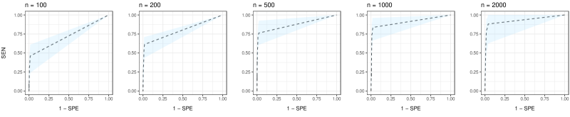
Regression
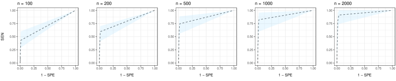
Block

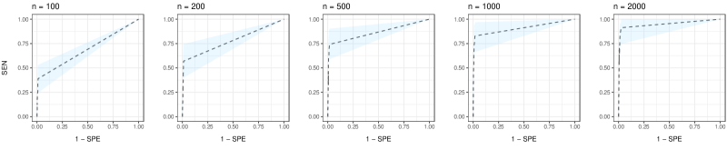
Figure 2: Simulations. Receiver operating characteristic (ROC) curve obtained under varying thresholds for the posterior probabilities of edge inclusion for type of variables Mixed $(b.4)$, sample size $n\in\{100,200,500,1000,2000\}$ $(c)$ and type of DAG structure Free, Regression, Block $(a)$. Dotted lines represent the (average over the 40 simulated DAGs) ROC curve, while the blue area represents the 5th-95th percentile band.

Free
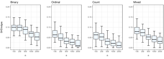
Regression
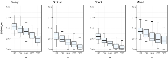
Block

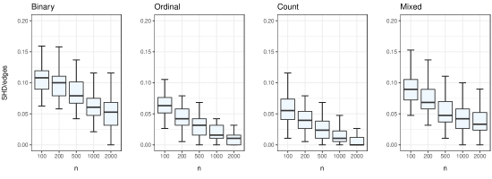
Figure 3: Simulations. Distribution (across $N=40$ simulated datasets) of the relative Structural Hamming Distance (SHD/edges) between estimated and true DAG for type of variables Binary, Ordinal, Count, Mixed $(b)$, sample size $n\in\{100,200,500,1000,2000\}$ $(c)$ and type of DAG structure Free, Regression, Block $(a)$.

Free
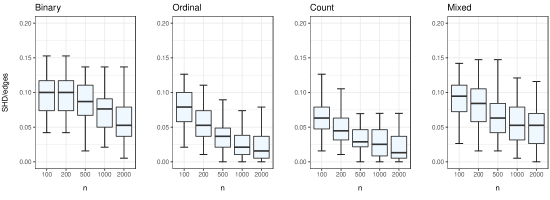
Regression
Block

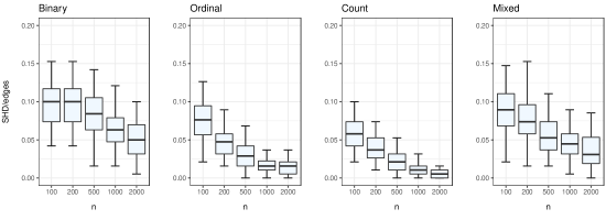
Figure 4: Simulations. Distribution (across $N=40$ simulated datasets) of the relative Structural Hamming Distance (SHD/edges) between estimated and true DAG for type of variables Binary, Ordinal, Count, Mixed $(b)$, sample size $n\in\{100,200,500,1000,2000\}$ $(c)$ and type of DAG structure Free, Regression, Block $(a)$.

We finally summarize in Tables 1 - 4 the Sensitivity (SEN) and Specificity (SPE) indexes computed under the median probability DAG model estimate. Each table refers to one scenario among Binary, Ordinal, Count, Mixed and reports the average (w.r.t. the $N=40$ simulations) percentage value of the two indexes under settings Free, Regression, Block corresponding to the three different classes of DAG structures. While SPE attains high levels even for small sample sizes, SEN significantly increases as $n$ grows. As a consequence, the improvement in the performance observed in Figure 3 is mainly due to a reduction in the inclusion of “false negative” edges as the number of available observations grows. In addition, it appears that DAG identification is somewhat easier under Scenarios Regression and Block. Here, structural constraints limiting the DAG space can help identifying dependence relations between variables which otherwise may not be uniquely identifiable because of DAG Markov equivalence (Andersson et al., 1997).

Table 1: Simulations. Binary data. Specificity (SPE) and sensitivity (SEN) indexes (averaged over the 40 simulations) computed w.r.t. the median probability DAG estimate, for sample size $n\in\{100,200,500,1000,2000\}$ and under each scenario Free, Regression, Block corresponding to different classes of DAG structures.

		Free			Regression			Block
$n$		SPE	SEN		SPE	SEN		SPE	SEN
100		100.00	0.00		100.00	0.00		100.00	0.00
200		100.00	3.04		100.00	4.55		99.72	5.41
500		99.16	32.74		99.16	30.38		99.16	32.74
1000		98.87	54.07		98.88	53.85		99.02	56.52
2000		98.74	67.26		98.87	69.40		98.87	71.01

Table 2: Simulations. Ordinal data. Specificity (SPE) and sensitivity (SEN) indexes (averaged over the 40 simulations) computed w.r.t. the median probability DAG estimate, for sample size $n\in\{100,200,500,1000,2000\}$ and under each scenario Free, Regression, Block corresponding to different classes of DAG structures.

		Free			Regression			Block
$n$		SPE	SEN		SPE	SEN		SPE	SEN
100		99.44	46.29		99.44	50.00		99.44	50.00
200		99.18	62.50		99.31	64.58		99.44	65.38
500		99.44	78.17		99.44	75.00		99.72	79.58
1000		99.43	85.10		99.44	87.50		99.72	89.06
2000		99.86	94.87		100.00	92.31		100.00	96.00

Table 3: Simulations. Count data. Specificity (SPE) and sensitivity (SEN) indexes (averaged over the 40 simulations) computed w.r.t. the median probability DAG estimate, for sample size $n\in\{100,200,500,1000,2000\}$ and under each scenario Free, Regression, Block corresponding to different classes of DAG structures.

		Free			Regression			Block
$n$		SPE	SEN		SPE	SEN		SPE	SEN
100		99.43	50.00		99.43	50.00		99.43	54.07
200		99.16	66.67		99.44	69.23		99.44	69.80
500		99.44	78.71		99.44	80.00		99.72	82.09
1000		99.45	88.12		99.72	88.87		99.86	91.11
2000		100.00	95.74		100.00	98.33		100.00	100.00

Table 4: Simulations. Mixed data. Specificity (SPE) and sensitivity (SEN) indexes (averaged over the 40 simulations) computed w.r.t. the median probability DAG estimate, for sample size $n\in\{100,200,500,1000,2000\}$ and under each scenario Free, Regression, Block corresponding to different classes of DAG structures.

		Free			Regression			Block
$n$		SPE	SEN		SPE	SEN		SPE	SEN
100		99.45	23.74		99.44	25.00		99.43	27.92
200		98.90	37.72		99.02	36.67		99.16	45.99
500		98.88	61.39		98.87	62.50		99.16	65.94
1000		98.89	71.01		98.86	73.68		99.01	74.46
2000		98.30	78.71		98.58	80.00		98.57	84.11

5.3 Simulation experiments with unbalanced correlation structure

In the simulation scenarios considered before we randomly drew the non-zero elements of matrix $\bm{L}$, corresponding to regression coefficients in the latent linear SEM, uniformly in the symmetric interval $[-1,-0.1]\cup[0.1,1]$. This implies an expected “balanced” correlation structure between variables, meaning that both positive and negative associations in the generating model will be present, and with same expected proportion. However, in many psychological applications variables are mostly positively correlated each other; see also our results in Section 6. An important example is represented by cognitive test scores, whose pattern of positive correlations was already advocated by Spearman (1904) in his positive manifold theory. To assess the ability of our method to capture such “unbalanced” correlation structure, we now consider a random choice of the non-zero elements of $\bm{L}$ in the interval $[0.1,1]$ and implement the same scenarios introduced in Section 5.1. Accordingly, all variables are now positively correlated at the latent level. Results, in terms of relative SHD between true and estimated DAG are reported in Figure 4, which summarizes the distribution of SHD across simulated datasets under all scenarios defined in Section 5.1. The performance of our method is in line with what observed in Figure 3, obtained under a balanced setting, suggesting that our model specification is insensitive to the specific proportion of positive/negative correlations.

6 Real data analyses

6.1 Well-being data

The Your Work-Life Balance is a project promoted by the United Nations (UN) and implemented through a public survey available at http://www.authentic-happiness.com/your-life-satisfaction-score. Scope of the survey is to evaluate how people thrive in both professional and personal lives based on several indicators that are related with life satisfaction. Variables considered in the study are classified into five dimensions:

• Healthy body, features reflecting fitness and healthy habits;

• Healthy mind, indicating how well subjects embrace positive emotions;

• Expertise, measuring the ability to grow expertise and achieve something unique;

• Connection, assessing the strength of social relationships;

• Meaning, evaluating compassion, generosity and happiness.

The survey supports the UN Sustainable Development Goals (https://sdgs.un.org) and aims at providing insights on the determinants of human well-being. Accordingly, some questions of interest are the following:

• “What are the strongest correlations between the various dimensions?”

• “What are the best predictors of a balanced life?”

The complete dataset is publicly available at https://www.kaggle.com/datasets/ydalat/lifestyle-and-wellbeing-data. It includes observations collected across years $2015-2020$ of $20$ ordinal variables (with levels ranging in $1-5$ or $1-10$) each measuring closeness of a subject w.r.t. to one perceived dimension, besides gender (binary) and age (ordinal with four classes). We include in our analysis the $n=459$ observations available for year $2020$. We consider variable stress as the response and accordingly allow edges from each of the remaining variables to the response only. In addition, age and gender are considered as objective features and accordingly cannot have incoming edges. We do not impose further constraints among the remaining variables in terms of edge directions that are known in advance.

Following the scope of the original project, we are interested in understanding how the various dimensions relate each other and what are the direct/indirect determinants of the perceived level of stress. To this end, we implement our MCMC algorithm for a number of iterations $S=20000$, after an initial burnin period of $5000$ runs that are discarded from posterior analysis. Diagnostic tools based on multiple chains and graphical inspections of the behavior across iterations of sampled parameters were also adopted to assess the convergence of the MCMC; see Section MCMC diagnostics of convergence and computational time for details.

We use the MCMC output to provide an estimate of the posterior probabilities of edge inclusion as well as a BMA estimate of the correlation matrix between (latent) variables. Results are reported in the two heat maps of Figure 5. The upper map, which collects the estimated posterior probabilities of edge inclusion clearly suggests a sparse structure in the underlying network, with only a few edges whose posterior probability exceeds $0.5$. This also emerges from the graph estimate reported in Figure 6, which corresponds to the CPDAG representing the equivalence class of the MPM DAG estimate.

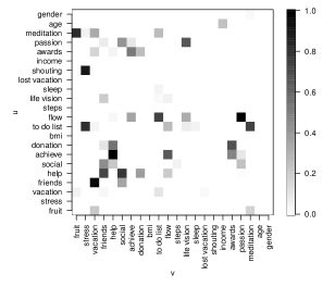
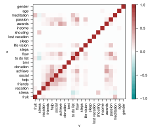
Figure 5: Well-being data. Upper panel: Heat map with estimated posterior probabilities of edge inclusion $\widehat{p}(u\rightarrow v\,|\,\bm{X})$ for each edge $(u,v)$. Lower panel: Estimated correlation matrix.

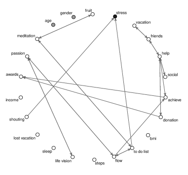
Figure 6: Well-being data. Estimated CPDAG.

The estimated graph reveals that two variables directly affect the perceived level of stress, namely shouting (“How often do you shout or sulk at somebody?”) and to do list (“how well do you complete your weekly to-do list?”). Moreover, variable stress is conditionally independent from flow (“How many hours you experience flow, i.e. you fell fully immersed in performing an activity?”) given to do list. Also, flow and to do list are positively correlated, which suggests that people performing better in their activities also follow through with many more of their weekly goals. This in turn has a direct impact on the perceived level of stress. It also appears that shouting is positively correlated with the level of stress, while there is negative correlation with to do list; accordingly better results in completing to-do-lists, imply a reduction in the stress level perceived by individuals.

6.2 Student mental health data

We consider a dataset from a cross-sectional study conducted on $886$ medical students in Switzerland and presented by Carrard et al. (2022). Target of the study is to provide insights on students’ well-being, in order to implement policies aimed at improving their academic-life satisfaction and conditions. A number of dimensions related to empathy are measured through self-reported questionnaires based on the Questionnaire of Cognitive and Affective Empathy (QCAE) and the Jefferson Scale of Physician Empathy (JSPE); related variables are the QCAE affective empathy score (qcae aff), the QCAE cognitive empathy score (qcae cog) and the JSPE total empathy score (jspe). Burnout is a state of emotional, physical, and mental exhaustion which is caused by excessive exposure to stress. The burnout dimension is measured through the Maslach Burnout Inventory-Student Survey (MBI-SS); the latter is based on $15$ items and provides three scores evaluating the following dimensions: emotional exhaustion (mbi ex), cynicism (mbi cy), and academic efficacy (mbi ea). In addition, students’ anxiety and depression is measured through the Center for Epidemiologic Studies Depression (CESD) score and the State-Trait Anxiety Inventory (STAI) score, both based on a questionnaire with self-report items on Likert scales (cesd and stai respectively). Finally, the dataset contains information on demographic factors such as age and gender, besides variables measuring job satisfaction (job), partnership status (part) and self-reported health status (health), represented by an ordinal variable with $5$ categories corresponding to increasing levels of perceived health satisfaction. We refer to Carrard et al. (2022) for a detailed description of the complete dataset, which is publicly available at https://zenodo.org/record/5702895. We emphasize that the structure of the analyzed dataset is quite heterogeneous, as it collects binary, ordinal (with different ranges of levels) as well as continuous measurements simultaneously.

One specific aim of the original study is to identify how variables included in the survey, in particular depressive symptoms, anxiety, and burnout, are related to empathy and mental health. In our analysis, we consider age, sex, part and job as exogenous variables, while we regard health as a response of interest.

Our MCMC algorithm is implemented for $S=20000$ iterations, after a burnin period of $5000$ runs that we adopt to assess the convergence of the chain. We use the MCMC output to provide an estimate of the (marginal) posterior probability of inclusion (PPI) for each possible directed edge in the DAG space; see Equation (23). The resulting heat-map with the collection of estimated PPIs (Figure 7, upper plot) suggests the existence of a few strong dependence relations among variables that correspond to directed links and paths in the graphs visited by the MCMC chain; this also appears from the MPM CPDAG estimate reported in Figure 8 which contains a moderate number of edges. Furthermore, to investigate how variables correlate each other, we provide a BMA estimate of the correlation matrix between (latent) variables (Figure 7, lower plot).

Notably, most variables belonging to the burnout dimension as well as to the anxiety or depression sphere are positively correlated with the exception of mbi ea, namely the score measuring academic efficacy, which as expected is negatively associated with the other variables, and in particular with the perceived level of anxiety (stai). mbi ea is also positively influenced by variable study (hours of study per week), which in turn has a positive, although less marked, effect on student’s anxiety. Importantly however, students’ depression, here quantified by the cesd score, has a negative effect on health, as it appears from the graph estimate of Figure 8 and the correlation matrix in Figure 7. Also, age has a positive impact on variable jspe which summarizes the empathy dimension, implying that medical students develop throughout their academic life a growing ability in understanding and sharing feelings that are experienced by others. Finally, an interesting set of structural dependencies is represented by the directed path study $\rightarrow$ stai $\rightarrow$ cesd $\rightarrow$ health. The latter structure suggests that students more involved in studying activities may incur in higher levels of anxiety and depression, which consequently affects personal health conditions.

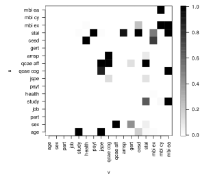
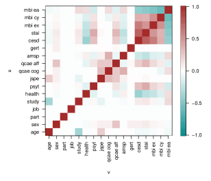
Figure 7: Student mental health data. Upper panel: Heat map with estimated posterior probabilities of edge inclusion $\widehat{p}(u\rightarrow v\,|\,\bm{X})$ for each edge $(u,v)$. Lower panel: Estimated correlation matrix.

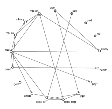
Figure 8: Student mental health data. Estimated CPDAG.

7 Discussion

We proposed a Bayesian semi-parametric methodology for structure learning of directed networks which applies to mixed data, i.e. data that include categorical, discrete and continuous measurements. Our model formulation assumes that the available observations are generated by latent variables whose joint distribution is multivariate Gaussian and satisfies the independence constraints imposed by a Directed Acyclic Graph (DAG). Following a copula-based approach, we model separately the dependence parameter and the marginal distributions of the observed variables which are estimated non-parametrically. The former corresponds to the covariance matrix, Markov w.r.t. an unknown DAG, for which a DAG-Wishart prior is assumed. Importantly, we fully account for model uncertainty by assigning a prior distribution to DAG structures. In addition, constraints on the network structure that are known beforehand can be easily incorporated in our model. The resulting framework allows for posterior inference on DAGs and DAG-parameters which is carried out by implementing an MCMC algorithm. We finally investigate the performance of our methodology through simulation studies. Results show that our method, when adopted to provide a single network estimate is highly competitive with the frequentist benchmark Copula PC. In addition, being Bayesian, uncertainty around network structures as well as dependence parameters is fully provided by our method.

The theory of latent traits assumes that available observations collected on subjects are associated to a (possibly small) number of latent individual characteristics (Hambleton & Cook, 1977). A latent trait model then establishes a mathematical relationship between these unobservable features and the observed data, which represent manifestations of the traits. In this context, Moustaki & Knott (2000) generalized the classical latent trait model, originally introduced for categorical manifest variables, to mixed data and specifically variables whose distribution belongs to the exponential family. For each manifest variable they specify a suitable generalized linear model, where covariates correspond to a set of common latent traits following independent normal distributions. Differently, our graphical modelling framework employs latent variables to project observable mixed-type features into a latent space (of same dimension) which, once equipped with a network model, incorporates a dependence structure between latent variables. We conjecture that our method could be extended to a latent trait framework for mixed data as the one considered by Moustaki & Knott (2000). A related model formulation would establish a link between each of the $q$ manifest variables and $K<q$ latent factors whose joint Gaussian distribution satisfies the conditional independencies embedded in a DAG. Finally, the method could identify a set of dependence relations between latent traits represented through a directed network.

Our model formulation assumes a common DAG structure with allied dependence parameter for all the available observations. In some settings however, a clustering structure may be present in the sample, with subjects divided into groups that are defined beforehand or unknown and therefore to learn from the data. In the former case, multiple datasets could be analyzed jointly by using a multiple graphical model approach (Peterson et al., 2015). The latter adopts a Markov random field prior that encourages common edges among group-specific graphs, and a spike-and-slab prior controlling network relatedness parameters. In the second case, one could instead set up a mixture model, where each mixture component corresponds to a possibly different network with allied parameters; as the output, a clustering structure of the subjects would be also available; see for instance Ickstadt et al. (2011) and Lee et al. (2022) for mixtures of graphical models in the Gaussian and ordinal framework respectively. Following a Bayesian non-parametric approach we could consider an infinite mixture model where each latent group is characterized by a component-specific parameter. A Dirichlet Process (prior) on the space of DAGs and DAG-parameters could be then assumed; see in particular Rodríguez et al. (2011) and Castelletti & Consonni (2023) for respectively undirected and directed Gaussian graphical models. Extensions of the proposed copula model to multiple DAGs and mixtures of DAGs are possible and currently under investigation.

Appendix

Comparison with Copula PC

In this section we compare our methodology with the benchmark Copula PC method of Cui et al. (2016); see also Cui et al. (2018). Copula PC is a two-step approach which can be applied to mixed data comprising categorical (binary and ordinal), discrete and continuous variables. It first estimates a correlation matrix in the space of latent variables (each associated with one of the observed variables) which is then used to test conditional independencies as in the standard PC algorithm. For the first step, the same Gibbs sampling scheme introduced by Hoff (2007) and based on data augmentation with latent observations is adopted. Moreover, conditional independence tests are implemented at significance level $\alpha$ which we vary in $\{0.01,0.05,0.10\}$; lower values of $\alpha$ imply a higher expected level of sparsity in the estimated graph. We refer to the three benchmarks as Copula PC 0.01, 0.05 and 0.10 respectively. Output of Copula PC is a Completed Partially Directed Acyclic Graph (CPDAG) representing the estimated equivalence class. With regard to our method, we also consider as a single graph estimate summarizing our MCMC output the CPDAG representing the equivalence class of the estimated median probability DAG model. Each model estimate is finally compared with the true CPDAG by means of the SHD between the two graphs.

Results for Scenario Free, type of variables Binary, Ordinal, Count, Mixed and each sample size $n\in\{100,200,500,1000,2000\}$ are summarized in Figure 9 which reports the distribution across $N=40$ simulations of the SHD. It first appears that all methods improve their performances as the sample size $n$ increases. In addition, structure learning is more difficult in the Binary case, while easier in general in the case of Ordinal and Count data. Moreover, Copula PC 0.01 (light grey) performs better than Copula PC 0.05 and 0.10 (middle and dark gray respectively). Our method clearly outperforms the three benchmarks in the Binary scenario, a behavior which is more evident for large sample sizes. In addition, it performs better than Copula PC 0.05 and 0.10 most of the time under the remaining settings and remains highly competitive with Copula PC 0.01, with an overall better performance in terms of average SHD under almost all sample sizes for Scenarios Ordinal and Count.

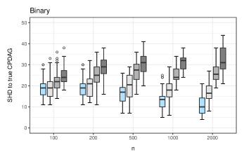
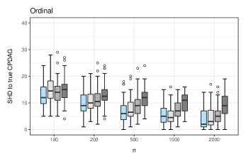
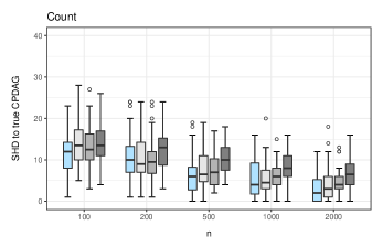
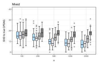
Figure 9: Simulations. Distribution (across $N=40$ simulated datasets) of the Structural Hamming Distance (SHD) between estimated and true CPDAG for type of variables Binary, Ordinal, Count, Mixed $(b)$, sample size $n\in\{100,200,500,1000,2000\}$ $(c)$ and type of DAG structure Free. Methods under comparison are: our Bayesian Copula DAG model (light blue) and the Copula PC method with independence tests implemented at significance level $\alpha\in\{0.01,0.0,0.10\}$ (from light to dark gray).

Comparison with Bayesian parametric strategy

Our methodology is based on a semi-parametric strategy which models separately the dependence parameter, corresponding to a DAG-dependent covariance matrix, and the marginal distributions of the observed variables, which are estimated using a rank-based non-parametric approach.

Alternatively, one can adopt appropriate parametric families for modeling the various mixed types of variables, as in a generalized linear model (glm) framework. To implement this parametric strategy, we generalize the latent Gaussian DAG-model in (1) to accommodate a non-zero marginal mean for the latent variables. Specifically, we assume

$$Z_{1},\dots,Z_{q}\,|\,\bm{\mu},\bm{\Omega},\mathcal{D}\sim\mathcal{N}_{q}(\bm{\mu},\bm{\Omega}^{-1}),$$ (25)

with $\bm{\mu}\in\mathbb{R}^{q}$ and $\bm{\Omega}\in\mathcal{P}_{\mathcal{D}}$, the space of all s.p.d. precision matrices Markov w.r.t. DAG $\mathcal{D}$. The allied Structural Equation Model (SEM) representation of such model is given by $\boldsymbol{\eta}+\bm{L}^{\top}\bm{z}=\boldsymbol{\varepsilon},\boldsymbol{\varepsilon}\sim\mathcal{N}_{q}(\bm{0},\bm{D})$, or equivalently, in terms of node-distributions

$$Z_{j}=\eta_{j}-\bm{L}_{\prec j\,]}^{\top}\bm{z}_{\mathrm{pa}_{\mathcal{D}}(j)}+\varepsilon_{j},\quad\varepsilon_{j}\stackrel{{\scriptstyle\textnormal{ind}}}{{\sim}}\mathcal{N}(0,\bm{D}_{jj}),$$ (26)

for each $j=1,\dots,q$ with $\bm{D}_{jj}=\bm{\Sigma}_{j\,|\,\mathrm{pa}_{\mathcal{D}}(j)},\bm{L}_{\prec j\,]}=-\bm{\Sigma}^{-1}_{\prec j\succ}\bm{\Sigma}_{\prec j\,]},\eta_{j}=\mu_{j}+\bm{L}^{\top}_{\prec j\,]}\bm{\mu}_{\mathrm{pa}_{\mathcal{D}}(j)}.$ Importantly, each equation in (26) now resembles the structure of a linear “regression” model with a non-zero intercept term $\eta_{j}$. A Normal-DAG-Wishart prior can be then assigned to $(\boldsymbol{\eta},\bm{D},\bm{L})$; see Castelletti & Consonni (2023, Supplement, Section 1) for full details. Under such prior, the posterior distribution of $(\boldsymbol{\eta},\bm{D},\bm{L})$ given independent (latent) Gaussian data $\bm{Z}$ is still Normal-DAG-Wishart and also a marginal data distribution is available in closed-from expression. Therefore, we can adapt the MCMC scheme of Section 4 to this more general framework and specifically with the update of $(\bm{D},\bm{L},\mathcal{D})$ in Section 4.1 replaced by $(\boldsymbol{\eta},\bm{D},\bm{L},\mathcal{D})$.

Consider now the observed variables $X_{1},\dots,X_{q}$, where each $X_{j}\sim F_{j}(\cdot)$, a suitably-specified parametric family for $X_{j}$, e.g. Bernoulli, Poisson, or Binomial; see also Section 4.1. As in a glm framework, we assume that

$$\mathbb{E}(X_{j}\,|\,\bm{z}_{\mathrm{pa}_{\mathcal{D}}(j)})=h^{-1}(\eta_{j}-\bm{L}_{\prec j\,]}^{\top}\bm{z}_{\mathrm{pa}_{\mathcal{D}}(j)})$$ (27)

where $h^{-1}(\cdot)$ is a suitable inverse-link function and it appears that $\eta_{j}-\bm{L}_{\prec j\,]}^{\top}\bm{z}_{\mathrm{pa}_{\mathcal{D}}(j)}$ plays the role of the linear predictor in the glm model for $X_{j}$. Specifically, we take $h(\cdot)=\textnormal{logit}(\cdot)$ and $h(\cdot)=\log(\cdot)$ for $X_{j}\sim\textnormal{Bern}(\pi_{j})$ and $X_{j}\sim\textnormal{Pois}(\lambda_{j})$ respectively. Moreover, for $X_{j}\sim\textnormal{Bin}(n_{j},\pi_{j})$ we take $h(\pi_{j})=\textnormal{logit}(\pi_{j})$ while fix $n_{j}=\max\{x_{i,j},i=1,\dots,n\}$. From (5) we then have $Z_{j}=\Phi^{-1}\left\{F_{j}(X_{j}\,|\,\bm{z}_{\mathrm{pa}_{\mathcal{D}}(j)})\right\},$ with $\Phi(\cdot)$ the standard normal c.d.f. and with $F_{j}$ implicitly depending on DAG parameters $(\eta_{j},\bm{L}_{\prec j\,]})$ through (27). The update of $\bm{Z}$ in Section 4.2 conditionally on the DAG parameters is then replaced by computing $z_{i,j}=\Phi^{-1}\left\{F_{j}(x_{i,j}\,|\,\bm{z}_{\mathrm{pa}_{\mathcal{D}}(j)})\right\}$ iteratively for each $i=1,\dots,n$ and $j=1,\dots,q$.

We consider the same simulation settings as in the Balanced Scenario, with the four different types of variables and with class of DAG structure Free; see Section 5.1. We compare the performance of the parametric strategy introduced above with our original method. Specifically, from the MCMC output provided by each method we first recover a CPDAG estimate and compare true and estimated graphs in terms of Structural Hamming Distance (SHD); see also Section 5.2 for details.

Results are summarized in the box-plots of Figure 10, representing the distribution of SHD (across the $40$ independent simulations) obtained from our original method (light blue) and its parametric version (dark blue) under the various scenarios. It appears that the parametric “version” of our method outperforms our original semi-parametric model in the Binary Scenario, while it is clearly outperformed under all the other scenarios for small-to-moderate sample sizes; however, the two approaches tend to perform similarly as the sample size $n$ increases.

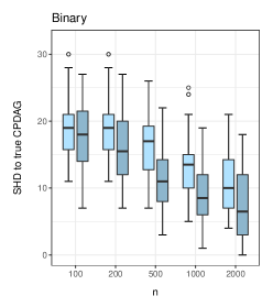
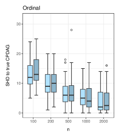
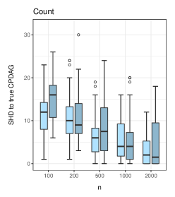
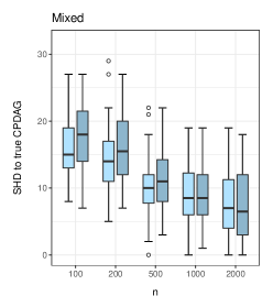
Figure 10: Simulations. Distribution (across $N=40$ simulated datasets) of the Structural Hamming Distance (SHD) between estimated and true CPDAG for type of variables Binary, Ordinal, Count, Mixed $(b)$, sample size $n\in\{100,200,500,1000,2000\}$ $(c)$ and type of DAG structure Free. Methods under comparison are: our original semi-parametric Bayesian Copula DAG model (light blue) and its modified version based on parametric assumptions (dark blue).

MCMC diagnostics of convergence and computational time

Our methodology relies on Markov Chain Monte Carlo (MCMC) methods to approximate the posterior distribution of the parameters. Accordingly, diagnostics of convergence of the resulting MCMC output to the target distribution should be implemented before posterior analysis. In the following we include a few results relative to the application of our method to the well-being datas presented in Section 6.1.

As a first diagnostic tool, we monitor the behavior of the estimated posterior expectation of each correlation coefficient across iterations. Each quantity is computed at MCMC iteration $s$ using the sampled values collected up to step $s$, for $s=1,\dots,25000$. According to the results, reported for selected variables $(X_{u},X_{v})$ in Figure 11, we discard the initial $B=5000$ draws that are therefore used as a burnin period. The behavior of each traceplot suggests for each parameter an appreciable degree of convergence to the posterior mean.

Figure 11: Well being data. Trace plots of the posterior mean of four correlation coefficients (for randomly selected variables $X_{u},X_{v}$) estimated from the MCMC output up to iteration $s$, for $s=1,\dots,25000$.

As a further diagnostic, we run two independent MCMC chains of length $S=25000$, again including a burnin period of $B=5000$ runs, and with randomly-chosen DAGs for the MCMC initialization. Results in terms of estimated posterior probabilities of edge inclusion computed from the two MCMC chains are reported in the heatmpas of Figure 12 and suggest a visible agreement between the two outputs.

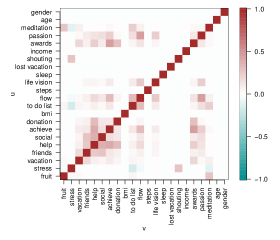
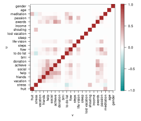
Figure 12: Well being data. Estimated correlation matrices obtained under two independent MCMC chains.

Finally, we investigate the computational time of our algorithm as a function of the number of variables $q$ and sample size $n$. The following plots summarize the behavior of the running time (averaged over $40$ replicates) per iteration, as a function of $q\in\{5,10,20,50,100\}$ for $n=500$, and as a function of $n\in\{50,100,200,500,1000\}$ for $q=20$. Results were obtained on a PC Intel(R) Core(TM) i7-8550U 1,80 GHz.

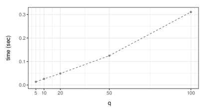
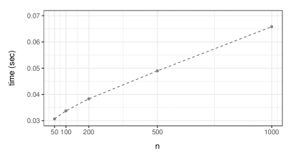
Figure 13: Computational time (in seconds) per iteration, as a function of the number of variables $q$ for fixed $n=500$ (upper plot) and as a function of the sample size $n$ for fixed $q=20$ (lower plot), averaged over $40$ simulated datasets.

References

- Andersson et al. (1997) Andersson, S. A., Madigan, D. & Perlman, M. D. (1997). On the Markov equivalence of chain graphs, undirected graphs, and acyclic digraphs. Scandinavian Journal of Statistics 24 81 – 102.
- Andrews et al. (2018) Andrews, B., Ramsey, J. & Cooper, G. F. (2018). Scoring Bayesian networks of mixed variables. International Journal of Data Science and Analytics 14 2 – 18.
- Andrews et al. (2019) Andrews, B., Ramsey, J. & Cooper, G. F. (2019). Learning high-dimensional directed acyclic graphs with mixed data-types. In Proceedings of Machine Learning Research, vol. 104 of Proceedings of Machine Learning Research. PMLR, 4 – 21.
- Barbieri & Berger (2004) Barbieri, M. M. & Berger, J. O. (2004). Optimal predictive model selection. The Annals of Statistics 32 870–897.
- Bhadra et al. (2018) Bhadra, A., Rao, A. & Baladandayuthapani, V. (2018). Inferring network structure in non-normal and mixed discrete-continuous genomic data. Biometrics 74 185 – 195.
- Borsboom (2008) Borsboom, D. (2008). Psychometric perspectives on diagnostic systems. Journal of clinical psychology 64 1089 – 1108.
- Borsboom et al. (2021) Borsboom, D., Deserno, M. K., Rhemtulla, M., Epskamp, S., Fried, E. I., McNally, R. J., Robinaugh, D. J., Perugini, M., Dalege, G., Jonasand Costantini, Isvoranu, A.-M., Wysocki, A. C., van Borkulo, C. D., van Bork, R. & Waldorp, L. J. (2021). Network analysis of multivariate data in psychological science. Nature Reviews Methods Primers 1 58.
- Briganti et al. (2022) Briganti, G., Scutari, M. & McNally, R. (2022). A tutorial on Bayesian networks for psychopathology researchers. Psychological Methods, Advance online publication NA – NA.
- Cao et al. (2019) Cao, X., Khare, K. & Ghosh, M. (2019). Posterior graph selection and estimation consistency for high-dimensional Bayesian DAG models. The Annals of Statistics 47 319 – 348.
- Carrard et al. (2022) Carrard, V., Bourquin, C., Berney, S., Schlegel, K., Gaume, J., Bart, P.-A., Preisig, M., Mast, M. S. & Berney, A. (2022). The relationship between medical students’ empathy, mental health, and burnout: A cross-sectional study. Medical Teacher 44 1392 – 1399.
- Castelletti & Consonni (2021) Castelletti, F. & Consonni, G. (2021). Bayesian causal inference in probit graphical models. Bayesian Analysis 16 1113 – 1137.
- Castelletti & Consonni (2023) Castelletti, F. & Consonni, G. (2023). Bayesian graphical modeling for heterogeneous causal effects. Statistics in Medicine 42 15 – 32.
- Castelletti et al. (2018) Castelletti, F., Consonni, G., Della Vedova, M. & Peluso, S. (2018). Learning Markov equivalence classes of directed acyclic graphs: an objective Bayes approach. Bayesian Analysis 13 1231 – 1256.
- Castelletti & Mascaro (2022) Castelletti, F. & Mascaro, A. (2022). BCDAG: An R package for Bayesian structure and Causal learning of Gaussian DAGs. arXiv pre-print URL https://arxiv.org/abs/2201.12003.
- Castelletti & Peluso (2021) Castelletti, F. & Peluso, S. (2021). Equivalence class selection of categorical graphical models. Computational Statistics & Data Analysis 164 107304.
- Cheng et al. (2017) Cheng, J., Li, T., Levina, E. & Zhu, J. (2017). High-dimensional mixed graphical models. Journal of Computational and Graphical Statistics 26 367 – 378.
- Chickering (2002) Chickering, D. M. (2002). Learning equivalence classes of Bayesian-network structures. Journal of Machine Learning Research 2 445 – 498.
- Cowell et al. (1999) Cowell, R. G., Dawid, P. A., Lauritzen, S. L. & Spiegelhalter, D. J. (1999). Probabilistic Networks and Expert Systems. New York: Springer.
- Cramer et al. (2010) Cramer, A. O. J., Waldorp, L. J., Van der Maas, H. L. J. & Borsboom, D. (2010). Comorbidity: a network perspective. Behavioral and brain sciences 33 137 – 150.
- Cui et al. (2018) Cui, R., Groot, P., & Heskes, T. (2018). Learning causal structure from mixed data with missing values using Gaussian copula models. Statistics and Computing 29 311 – 333.
- Cui et al. (2016) Cui, R., Groot, P. & Heskes, T. (2016). Copula PC algorithm for causal discovery from mixed data. In P. Frasconi, N. Landwehr, G. Manco & J. Vreeken, eds., Machine Learning and Knowledge Discovery in Databases. Cham: Springer International Publishing, 377–392.
- Dobra & Lenkoski (2011) Dobra, A. & Lenkoski, A. (2011). Copula Gaussian graphical models and their application to modeling functional disability data. The Annals of Applied Statistics 2A 969 – 993.
- Edwards (2000) Edwards, D. (2000). Introduction to Graphical Modelling. New York: Springer.
- Epskamp et al. (2017) Epskamp, S., Kruis, J. & Marsman, M. (2017). Estimating psychopathological networks: Be careful what you wish for. PLOS ONE 12 1 – 13.
- Friedman et al. (2008) Friedman, J., Hastie, T. & Tibshirani, R. (2008). Sparse inverse covariance estimation with the graphical lasso. Biostatistics 9 432 – 441.
- Godsill (2012) Godsill, S. J. (2012). On the relationship between markov chain monte carlo methods for model uncertainty. Journal of Computational and Graphical Statistics 10 230 – 248.
- Hambleton & Cook (1977) Hambleton, R. K. & Cook, L. L. (1977). Latent trait models and their use in the analysis of educational test data. Journal of Educational Measurement 14 75–96.
- Harris & Drton (2013) Harris, N. & Drton, M. (2013). PC algorithm for nonparanormal graphical models. Journal of Machine Learning Research 14 3365 – 3383.
- Haslbeck & Waldorp (2018) Haslbeck, J. M. B. & Waldorp, L. J. (2018). How well do network models predict observations? on the importance of predictability in network models. Behavior Research Methods 50 853 – 861.
- He et al. (2017) He, Y., Zhang, X., Wang, P. & Zhang, L. (2017). High dimensional Gaussian copula graphical model with FDR control. Computational Statistics & Data Analysis 113 457 – 474.
- Heckerman et al. (1995) Heckerman, D., Geiger, D. & Chickering, D. M. (1995). Learning Bayesian networks: The combination of knowledge and statistical data. Machine Learning 20 197 – 243.
- Hoeting et al. (1999) Hoeting, J. A., Madigan, D., Raftery, A. E. & Volinsky, C. T. (1999). Bayesian model averaging: A tutorial. Statistical Science 14 382–401.
- Hoff (2007) Hoff, P. (2007). Extending the rank likelihood for semiparametric copula estimation. The Annals of Applied Statistics 1 265 – 283.
- Ickstadt et al. (2011) Ickstadt, K., Bornkamp, B., Grzegorczyk, M., Wieczorek, J., Sheriff, M. R., Grecco, H. E. & Zamir, E. (2011). Nonparametric Bayesian networks. In J. M. Bernardo, M. J. Bayarri, J. O. Berger, A. P. Dawid, D. Heckerman, A. F. M. Smith & M. West, eds., Bayesian Statistics 9. Oxford University Press, 283 – 316.
- Isvoranu et al. (2022) Isvoranu, A., Epskamp, S., Waldorp, L. J. & Borsboom, D. E. (2022). Network psychometrics with R: A guide for behavioral and social scientists. Routledge, New York.
- Kalisch & Bühlmann (2007) Kalisch, M. & Bühlmann, P. (2007). Estimating high-dimensional directed acyclic graphs with the PC-algorithm. Journal of Machine Learning Research 8 613 – 636.
- Lauritzen (1996) Lauritzen, S. L. (1996). Graphical Models. Oxford University Press.
- Lauritzen & Wermuth (1989) Lauritzen, S. L. & Wermuth, N. (1989). Graphical models for associations between variables, some of which are qualitative and some quantitative. The Annals of Statistics 17 31 – 57.
- Lee & Hastie (2013) Lee, J. & Hastie, T. (2013). Structure learning of mixed graphical models. In C. M. Carvalho & P. Ravikumar, eds., Proceedings of the Sixteenth International Conference on Artificial Intelligence and Statistics, vol. 31 of Proceedings of Machine Learning Research. Scottsdale, Arizona, USA: PMLR, 388 – 396.
- Lee et al. (2022) Lee, K. H., Chen, Q., DeSarbo, W. S. & Xue, L. (2022). Estimating finite mixtures of ordinal graphical models. Psychometrika 87 83 – 106.
- Liu et al. (2009) Liu, H., Lafferty, J. & Wasserman, L. (2009). The nonparanormal: Semiparametric estimation of high dimensional undirected graphs. Journal of Machine Learning Research 10 2295–2328.
- Maathuis & Nandy (2016) Maathuis, M. & Nandy, P. (2016). A review of some recent advances in causal inference. In P. Bühlmann, P. Drineas, M. Kane & M. van der Laan, eds., Handbook of Big Data. Chapman and Hall/CRC, 387 – 408.
- Marsman et al. (2022) Marsman, M., Huth, K., Waldorp, L. J. & Ntzoufras, I. (2022). Objective Bayesian edge screening and structure selection for Ising networks. Psychometrika 87 47 – 82.
- Marsman & Rhemtulla (2022) Marsman, M. & Rhemtulla, M. (2022). Guest Editors’ introduction to the special issue “Network Psychometrics in action”: Methodological innovations inspired by empirical problems. Psychometrika 87 1 – 11.
- Meinshausen & Bühlmann (2006) Meinshausen, N. & Bühlmann, P. (2006). High-dimensional graphs and variable selection with the Lasso. The Annals of Statistics 34 1436 – 1462.
- Mohammadi et al. (2017) Mohammadi, A., Abegaz, F., van den Heuvel, E. & Wit, E. C. (2017). Bayesian modelling of Dupuytren disease by using Gaussian copula graphical models. Journal of the Royal Statistical Society: Series C (Applied Statistics) 66 629 – 645.
- Moustaki & Knott (2000) Moustaki, I. & Knott, M. (2000). Generalized latent trait models. Psychometrika 65 391 – 411.
- Müller & Czado (2019) Müller, D. & Czado, C. (2019). Dependence modelling in ultra high dimensions with vine copulas and the graphical lasso. Computational Statistics & Data Analysis 137 211 – 232.
- Ni et al. (2022) Ni, Y., Baladandayuthapani, V., Vannucci, M. & Stingo, F. C. (2022). Bayesian graphical models for modern biological applications. Statistical Methods & Applications 31 197 – 225.
- Pearl (2000) Pearl, J. (2000). Causality: Models, Reasoning, and Inference. Cambridge University Press, Cambridge.
- Peluso & Consonni (2020) Peluso, S. & Consonni, G. (2020). Compatible priors for model selection of high-dimensional Gaussian DAGs. Electronic Journal of Statistics 14 4110 – 4132.
- Peterson et al. (2015) Peterson, C., Stingo, F. C. & Vannucci, M. (2015). Bayesian inference of multiple Gaussian graphical models. Journal of the American Statistical Association 110 159 – 174.
- Rodríguez et al. (2011) Rodríguez, A., Lenkoski, A. & Dobra, A. (2011). Sparse covariance estimation in heterogeneous samples. Electronic Journal of Statistics 5 981 – 1014.
- Scott & Berger (2010) Scott, J. G. & Berger, J. O. (2010). Bayes and empirical-Bayes multiplicity adjustment in the variable-selection problem. The Annals of Statistics 38 2587 – 2619.
- Spearman (1904) Spearman, C. (1904). General intelligence, objectively determined and measured. The American Journal of Psychology 15 201–292.
- Spirtes et al. (2000) Spirtes, P., Glymour, C. & Scheines, R. (2000). Causation, prediction and search (2nd edition). Cambridge, MA: The MIT Press. 1 – 16.