1D-CNN Optimization for Non-contact
Respiration Pattern Classification

Abstract

In this study, we present a deep learning-based approach for time-series respiration data classification. The dataset contains regular breathing patterns as well as various forms of abnormal breathing, obtained through non-contact incoherent light-wave sensing (LWS) technology. Given the one-dimensional (1D) nature of the data, we employed a 1D convolutional neural network (1D-CNN) for classification purposes. Genetic algorithm was employed to optimize the 1D-CNN architecture to maximize classification accuracy. Addressing the computational complexity associated with training the 1D-CNN across multiple generations, we implemented transfer learning from a pre-trained model. This approach significantly reduced the computational time required for training, thereby enhancing the efficiency of the optimization process. This study contributes valuable insights into the potential applications of deep learning methodologies for enhancing respiratory anomaly detection through precise and efficient respiration classification.

I Introduction

Human respiratory rate and its pattern convey valuable information about the physical and mental states of the subject. Anomalous breathing can be indicative of serious health issues such as asthma, obstructive sleep apnea, bronchitis, emphysema, lung cancer, chronic obstructive pulmonary disease, COVID-19, etc. It can also serve as a precursor to unstable mental conditions, including stress, panic, anxiety, fatigue, anger, etc. Contact-based monitoring falls short in capturing the true essence of one’s breathing, as individuals may alter their breathing patterns when aware of being monitored. Furthermore, subjects may be too young or too ill (such as patients with contagious diseases or those in burn units) to apply contact-based approaches for an extended duration. Current automated technologies for non-contact breathing monitoring typically rely on sensing electromagnetic signals, such as radar [1, 2, 3, 4], WiFi [5, 6, 7, 8], or extracting breathing information from videos captured by red-green-blue (RGB) [9, 10, 11, 12, 13] or thermal infrared cameras [14, 15, 16, 17]. We have developed a non-contact respiration monitoring system based on sensing incoherent infrared (IR) light reflected from the subject’s chest. This technology surpasses existing methods due to the safe, ubiquitous, and discreet nature of infrared light, avoiding privacy issues associated with camera-based approaches. The main functional components of the system include the LWS hardware, signal processing, and feature extraction algorithms, along with classification algorithms. Infrared LED sources illuminate the subject’s chest, and the reflected light’s intensity, varying with chest movement, is captured and converted into electrical voltage by a commercially available photodetector. Collected data are processed to extract features using signal processing algorithms and then classified using machine learning models.

Classifying 1D respiration data for respiratory anomaly detection is a crucial task in healthcare. Traditional machine learning models, including decision tree, random forest, K-nearest neighbor, and support vector machine, have been commonly employed for this purpose. However, these models heavily rely on handcrafted features, necessitating domain expertise and environment-specific additional measurements. This dependence can be considered an overhead in live implementation [18]. In contrast, deep learning models, such as 1D-CNNs, have shown promise in automatically extracting subtle features, including those imperceptible to humans. Leveraging convolutional layers for feature extraction and fully connected layers for classification, 1D-CNNs offer a more suitable approach for real-life implementation. Consequently, this study explores the application of 1D-CNNs for the classification of respiration data.

Neural architecture search, a prominent research area, aims to identify the most optimal neural network architecture for specific tasks. While random search is not always guaranteed to yield an optimal model, it is not uncommon in the literature [19, 20]. Genetic algorithm (GA) [21], renowned for single and multi-objective optimization tasks, has shown promise in neural architecture search [22, 23]. Various GA variants have been utilized for CNN optimization in diverse applications, such as fault diagnosis of hydraulic piston pumps, Alzheimer’s disease diagnosis, and stock market prediction [24, 25, 26]. In the current study, 1D-CNN is employed to classify respiration data into 8 different classes, including a class dedicated to faulty data detection. The architecture of the 1D-CNN is optimized to maximize test accuracy through a genetic algorithm developed from scratch in Python. To minimize computational complexity, transfer learning is employed from a pre-trained 1D-CNN model, enabling efficient execution of the genetic algorithm across multiple generations.

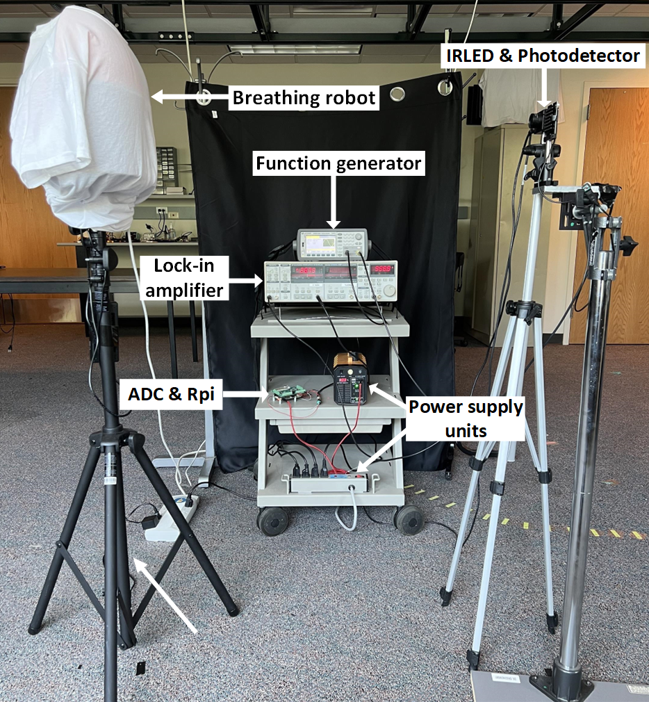
Figure 1: The hardware setup of the overall system used for data collection.

The remainder of this manuscript is organized as follows. Section II describes the system model including hardware setup and software algorithms to collect breathing data of different classes and perform classification. Section III presents the details of 1-dimensional convolutional neural network (1D-CNN) optimization including the application of transfer learning in subsection III-A and genetic algorithm (GA) in subsection III-B. Next, Section IV presents the results and discussion from GA and final breathing classification using the obtained optimized model. Finally, Section V draws conclusions from the effort and forecasts future research directions.

II System Design and Implementation

II-A Experimental setup

Human subjects typically cannot replicate breathing with precise frequency, amplitude, and patterns consistently. Therefore, a mechanical robot capable of simulating human breathing in various programmable patterns was developed and utilized for this study. The LWS sensing hardware includes infrared light sources as transmitters, a photodetector as the receiver, a digital signal processing (DSP) unit to convert the received signal from analog to digital, and an electronic module for processing and storing the digital data. Additionally, a function generator and lock-in amplifier were used to for coherent detection of the received light. The light source utilized was an invisible 940 nm IR lamp board (48 black LED illuminator array), offering a range of 30 ft and a wide beamwidth of 120° wide beamwidth [27]. The light source was modulated by a 1 kHz sinusoidal voltage wave from a function generator. The receiver employed was a commercial photodetector, Thorlabs PDA100A [28] with a converging lens. For lock-in detection, SR830DSP frequency lock-in amplifier [29] was utilized. A Raspberry Pi, equipped with a PiPlate analog-to-digital converter (ADC) circuit [30], managed the data collection, digitization, and storage for subsequent offline processing. The complete experimental setup is illustrated in Fig. 1.

TABLE I: Characteristics and number of collected data of each breathing class

Class	Class name	Breathing rate (BPM)	Breathing depth (%)	Number of data instances
0	Eupnea	12-20	30-58	300
1	Apnea	0	0	300
2	Tachypnea	21-50	30-58	300
3	Bradypnea	1-11	30-58	300
4	Hyperpnea	12-20	59-100	300
5	Hypopnea	12-20	1-29	300
6	Kussmaul’s	21-50	59-100	300
7	Faulty data	Any	Any	300
Total				2400

II-B Data collection

To gather respiration data, the infrared light emitted by the LED source underwent modulation using a sinusoidal voltage wave at 1 kHz with a peak-to-peak amplitude of 3.8 V and a DC offset of 8.1 V from the function generator. These specific voltage parameters were chosen to ensure linear LED operation with sufficiently high light intensity. The reflected light was captured by a photodetector paired with a converging lens having a focal length of 25.4 mm. The photodetector’s gain was set to 40 dB. The output from the photodetector was linked to a lock-in amplifier with a time constant of 100 ms. The resulting filtered signal from the lock-in amplifier was then digitized by the ADC. Finally, a Python script executed on the Raspberry Pi collected and stored the voltage amplitude data, along with their corresponding timestamps.

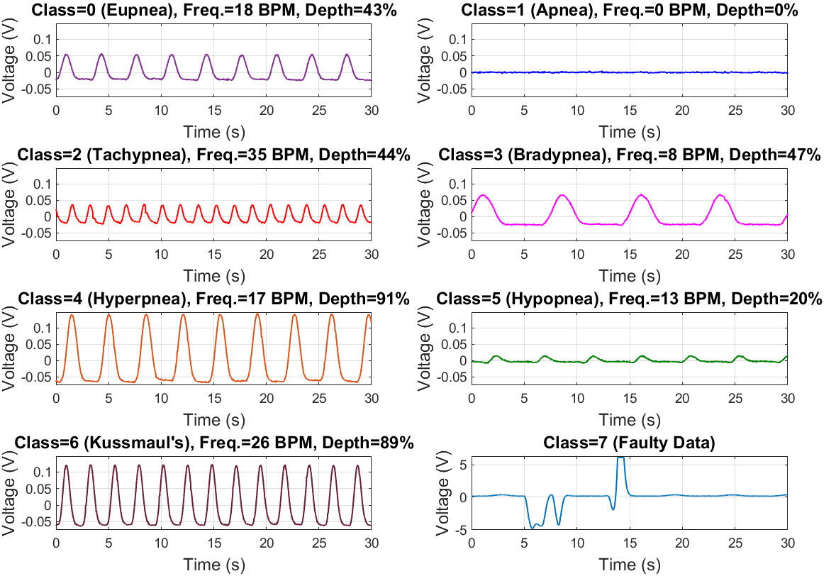
Figure 2: Time domain representation of sample data from each class (the distance between the source-photodetector and the robot was 1 m).

From the literature, 7 different classes of human breathing were identified and their characteristics, in terms of breathing rate (frequency) and depth (amplitude), were summarized in Table I [32, 4, 31, 33, 34, 14, 35, 36, 37, 38, 39, 40]. One of them (Eupnea) was normal breathing, while the rest were examples of different categories of abnormal breathing. The robot was programmed to breathe with frequencies and amplitudes in the appropriate ranges according to Table I to generate data experimentally for each class. Data for one additional class called ‘faulty data’ were generated too by manually interrupting the system or the surroundings during data collection. This class was introduced to detect erroneous data generated due to possible internal or external malfunction so that they can be discarded and recollected. $\sin^{6}$ waveform seemed to have the closest match with human breathing in terms of inspiration and expiration time, hence this pattern was used in the robot for all breathing classes. A total of 2400 data instances (300 per class) were collected during the daytime, keeping the windows of the room unshaded and internal lighting common for an office environment. For each class, 100 data instances were collected at 0.5 m, 1 m and 1.5 m distances each. Each data was 30 s long and collected at 100 Hz sampling frequency. All the collected data were saved along with their class labels (0 to 7) for further offline processing. Fig. 2 shows the time domain waveforms of a few samples of raw data, one from each class, collected at 1 m distance.

The raw data went through offline signal processing which includes moving average filtering (50 points) to suppress noise and a 5-th order polynomial detrending to remove upward or downward trends that were in some data instances. Thus, the data were prepared for feeding them to 1-dimensional convolutional neural network (CNN) for feature extraction and classification.

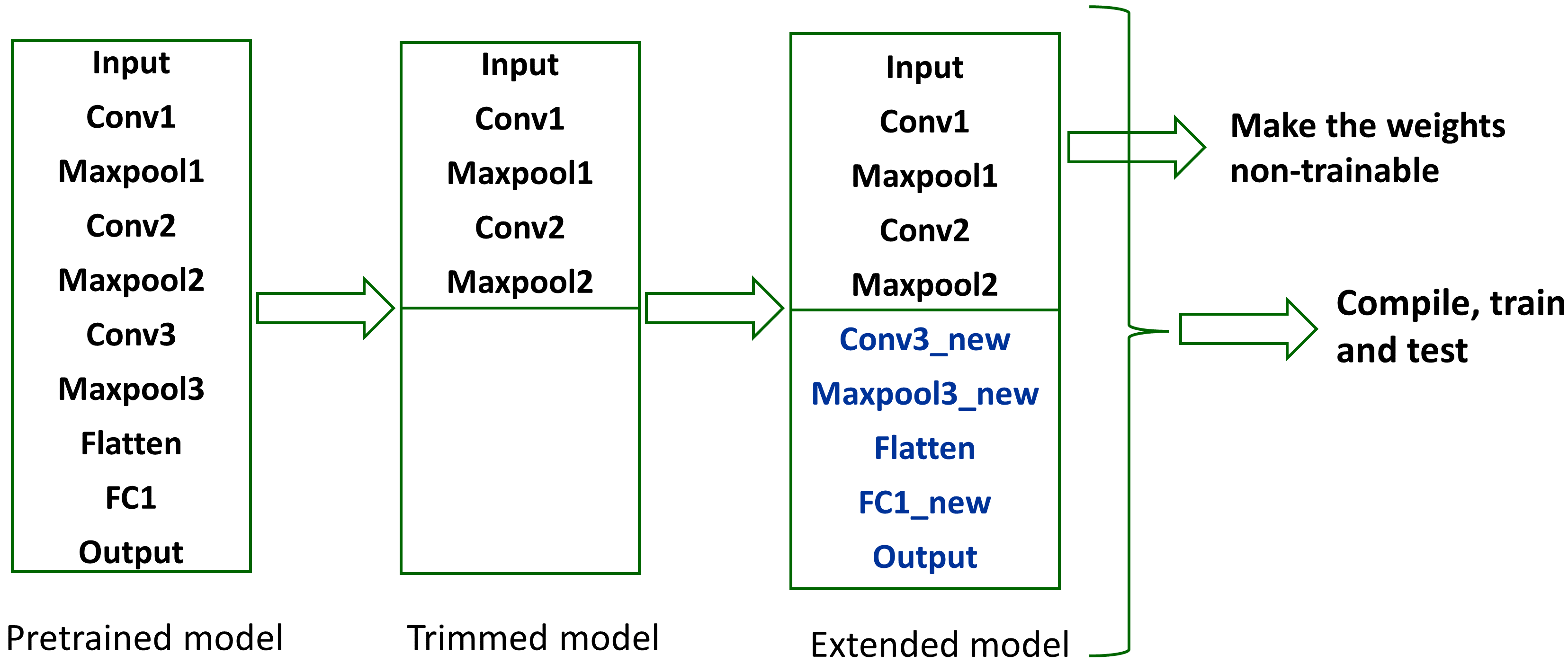
Figure 3: pre-trained, trimmed and extended models.

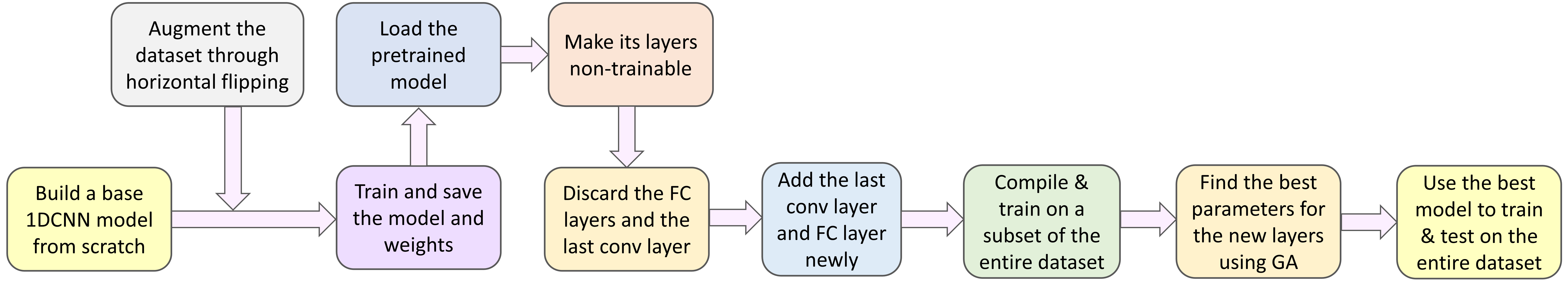
Figure 4: Transfer learning framework for 1-dimensional respiration data classification.

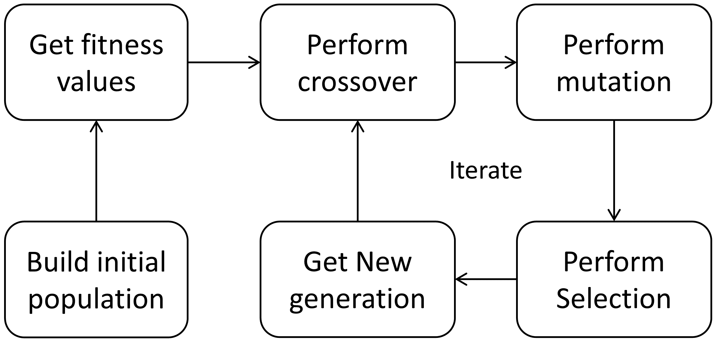
Figure 5: Genetic algorithm workflow.

III 1D-CNN Optimization

Given that the respiratory data is one-dimensional, the application of a 1D-CNN with one-dimensional filters for convolution becomes a viable choice. Leveraging the Keras API in Python, the data is processed through a 1D CNN model. The 1D-CNN model may have various potential architectures, each resulting in different accuracies for respiration classification. To optimize accuracy, it becomes imperative to identify the most suitable architecture. The utilization of a genetic algorithm (GA) is proposed to fine-tune the parameters of the 1D-CNN model, aiming to achieve an optimal architecture. However, the evaluation of fitness values for numerous solutions or 1D-CNN architectures is computationally expensive. To address this challenge, transfer learning has been incorporated into this study. By leveraging transfer learning, the computational burden is significantly reduced, enabling the execution of the genetic algorithm over a sufficient number of generations.

III-A Transfer Learning Application

Transfer learning is a powerful paradigm in machine learning that leverages knowledge gained from solving one task to improve the performance on a different, but related, task. In essence, it allows a model trained on one dataset to be fine-tuned or adapted for a different but similar task. This approach is particularly beneficial when the target task has limited labeled data, as it enables the model to generalize better. It is also useful to make the training faster through utilizing pre-trained weights. In the context of deep learning, transfer learning is often applied using pre-trained neural network architectures, such as those trained on large-scale image datasets like ImageNet [41]. The model’s initial layers learn generic features like edges and textures, while the deeper layers capture more task-specific information. This modular structure facilitates the reuse of the pre-trained layers for a new task. For instance, in Python, utilizing transfer learning with TensorFlow library involves loading pre-trained models like VGG16 [42] or ResNet [43] and adapting them for specific tasks with minimal effort. This accelerates training and enhances performance, making transfer learning a valuable tool in the machine learning toolbox.

Although many famous 2D-CNN models pre-trained on ImageNet dataset are available as API for direct use, their 1D counterparts are rare in the literature and GitHub repositories [20]. To address this problem, a single 1D-CNN model was obtained through random search that yields higher classification accuracy than most of the other tested models. The complete architecture of that model is shown in the leftmost bounded box in Fig. 3 and described as follows:

1. Input layer: It was a breathing data vector (1, 3000) pulled from the rows of the overall data matrix.

2. Convolutional layer 1: It was the first convolutional layer. 256 1D filters of length 64 were used to perform convolution in this layer. Spatial dimensions of data were preserved using padding =“same”. ‘Relu’ was used as the activation function.

3. Maxpooling layer 1: This layer took 2 data points repeatedly from the previous layer and replaced it by the maximum value. So, it had length 2 and stride 2.

4. Convolutional layer 2: It was the second convolutional layer. 128 1D filters of length 32 were used to perform convolution in this layer. Similar padding and activation function was used as the first convolutional layer.

5. Maxpooling layer 2: This layer is exactly the same as the first maxpooling layer

6. Convolutional layer 3: It was the third convolutional layer. 64 1D filters of length 16 were used to perform convolution in this layer. Similar padding and activation function was used as the first and second convolutional layers.

7. Maxpooling layer 3: This layer is exactly the same as the first and second maxpooling layers.

8. Flattened layer: The resulting data were flattened for feeding it to the fully connected (FC) layer.

9. Fully connected layer 1: The flattened data was passed through a fully connected neural layer. The hidden layer had 64 neurons. ‘Relu’ was used as the activation function.

10. Output layer: It was the final output layer with ‘softmax’ activation function which had 8 neurons, one for each class.

Next, this model was trained for 30 epochs and the trained model and weights were stored as pre-trained model. It is common in transfer learning to apply data augmentation to increase the number of training data and improve generalization. For image dataset, various affine transformations like rotation, shearing etc. are applied to produce new data instances [44, 45]. In our case, we not only utilized the whole respiration dataset of 2400 data instances, but also doubled the number of data through horizontal flipping. Since the respiration simulated by the robot was symmetric, following a $\text{sin}^{6}$ pattern, horizontal flipping generated valid respiration data. Then the combined 4800 instances of data (with 80%-20% train-test split) were fed to the 1D-CNN model for training. After that, the pre-trained model and weights were saved in .h5 format. The overall approach followed for transfer learning part is presented in Fig. 4.

III-B Optimization Using Genetic Algorithm

Genetic algorithm was applied using Python to find the optimum 1D-CNN model from a chosen solution space through crossovers and mutations over generations of solutions. Since transfer learning was applied to preload part of the CNN model in trained status, GA was used mainly to tune the rest of the model. The high level workflow of the genetic algorithm applied was shown in Fig. 5, but it involved some advanced features too which will be discussed here.

At first, the saved pre-trained model was loaded. Then, as depicted in Fig. 3, the output layer, FC layer, flattened layer and the last convolutional and maxpooling layers were removed. After that, similar untrained layers were added newly to construct the extended model (Fig. 3). The weights of the pre-trained part were made non-trainable, because these should not change during the new training runs. Next, GA was applied to choose parameters for the untrained part to maximize the classification accuracy. A subset of the entire data set (1000 data instances with 80%-20% train-test split) was used for applying GA to make the training processes faster.

III-B1 Build Chromosome and Initial Population

The first step was to decide the chromosome structure or genotypes of each gene and define their corresponding phenotypes or how they relate to the 1D-CNN architecture. Our chromosome contains four genes as shown in Fig. 6. We used all parameters as powers of 2 because these numbers create more computationally efficient model. First gene denotesd the number of kernels for the newly added convolutional layer and is a random integer number between 3 to 8. If the integer generated is 6, then the number of kernels for that layer will be $2^{6}=64$. Second gene denotes the length of kernels and is an integer between 2 to 6, or equivalently kernel length varied between $2^{3}$ and $2^{6}$. The third gene represents the maxpooling size and the fourth gene indicates the number of neurons present in the fully connected layer.

III-B2 Get Fitness Values

In every iterations of GA, new parameters for the untrained part were chosen for each solutions, and the combined model was compiled, trained on training dataset and finally tested on test dataset to get the fitness value. Only one epoch was used for each solution, with a batch size 50, to save computational time. The obtained test accuracy is defined to be the reproductive fitness value.

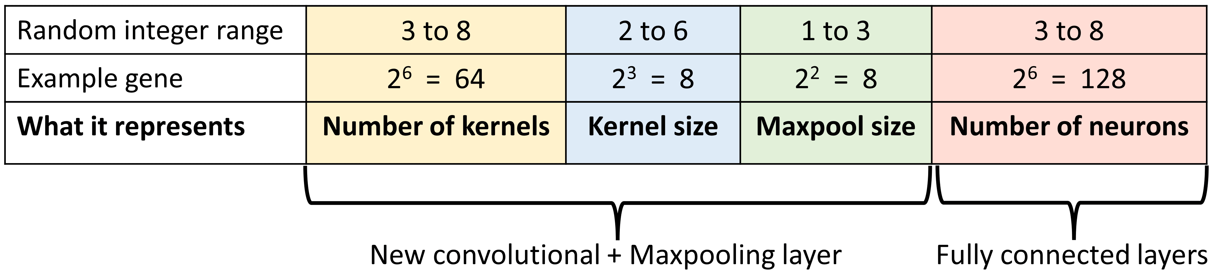
Figure 6: Chromosome for GA.

III-B3 Perform Crossover

3 single-point crossovers were performed on the chromosomes each having crossover probability 0.8 in each generation. We tried two approaches to select parents for crossover operations. Firstly, the highest fitness 6 individuals were chosen who went through crossover to produce offsprings. Secondly, a Roulette Wheel selection technique was adopted to select parents so that all individuals got at least some chance to be selected.

III-B4 Perform Mutation

Frequent mutation might prohibit convergence by losing the best solutions, hence only 1 individual went through mutation in each generation with a lower probability (0.4). In each mutation operation, only 1 gene was altered in the chromosome.

III-B5 Perform Selection

Roulette wheel selection was used to select 8 individuals from the combined list of individuals of current and previous generations. While doing this, 2 best fitness individuals were preserved through elitism. If there were any duplicate chromosomes in the selected individuals, then they were replaced by randomly generated new chromosomes.

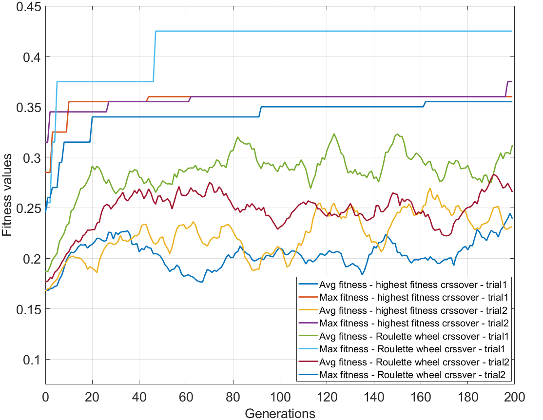
Figure 7: Maximum and average classification accuracy on the chosen subset of data after one epoch (defined as reproductive fitness) vs. number of generations of solutions

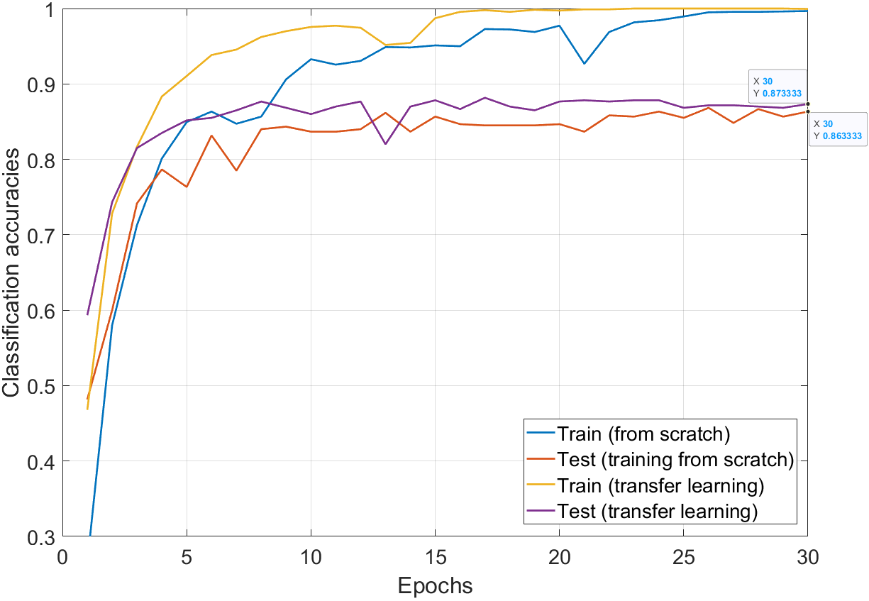
Figure 8: Training and testing accuracy plotted against the number of epochs. The training was performed by feeding the entire breathing dataset to the optimized 1D-CNN model found through GA.

IV Results and Discussions

The results from a few trial runs of GA up to 200 generations are displayed in Fig. 7. It shows how the maximum fitness and the average fitness evolves over generations. 2 trials are shown with highest fitness individuals selected as crossover parents, while 2 more are shown with Roulette wheel selection for selecting parents for crossover. Average fitness values fluctuate frequently, hence 10 points moving average filtering was performed to see the trend. Although the average fitness values are slowly increasing, there is clear increasing trend in the maximum fitness values. Trial 1 with the Roulette wheel parents selection for crossover yielded the highest fitness value 0.43 or 43% classification accuracy after 1 epoch. The corresponding chromosome was [7, 5, 1, 8] and this was chosen as the best solution to test on the entire dataset over many epochs. This solution was combined with the pre-trained part of the model and then the entire model was trained on the available 2400 data instances (without augmentation this time) for 30 epochs. Two distinct training approaches were employed: one involving training the model from scratch with no pre-trained weights, and the other incorporating transfer learning. The latter utilized pre-trained weights for the initial layers, while training only the remaining layers. The training and test accuracies as a function of number of epochs for both scenarios are plotted in Fig. 8. TNotably, the achieved test accuracies were comparable in both training methods, with a slightly higher accuracy (87.33%, compared to 86.33%) observed when incorporating transfer learning in the final training.

V Conclusion and Future Directions

In conclusion, deep learning model like 1D-CNN was found to be effective in respiration data classification which paves the way to respiratory anomaly detection and improves health monitoring at both home and clinics. To further alleviate computational complexity, there is an opportunity to execute the genetic algorithm code exclusively on GPU, leveraging its parallel processing capabilities. More sophisticated data augmentation can be performed beyond horizontal flipping to enhance the dataset for base model training further which will improve the pre-trained weights. The problem can be made multi-objective by including a second objective of minimizing the number of trainable parameters in the 1D-CNN architecture and non-dominated sorting genetic algorithm (NSGAII) can be applied to find the optimum model.

References

- [1] J. Salmi and A. F. Molisch, “Propagation parameter estimation, modeling and measurements for ultrawideband MIMO radar,” IEEE Transactions on Antennas and Propagation, vol. 59, no. 11, pp. 4257–4267, 2011.
- [2] D. Kocur, D. Novák, and J. Demčák, “A joint localization and breathing rate estimation of static persons using UWB radar,” in 2017 IEEE International Conference on Systems, Man, and Cybernetics (SMC), 2017, pp. 1728–1733.
- [3] F. Adib, H. Mao, Z. Kabelac, D. Katabi, and R. C. Miller, “Smart homes that monitor breathing and heart rate,” in Proceedings of the 33rd annual ACM conference on human factors in computing systems, 2015, pp. 837–846.
- [4] A. T. Purnomo, D. B. Lin, T. Adiprabowo, and W. F. Hendria, “Non-contact monitoring and classification of breathing pattern for the supervision of people infected by COVID-19,” Sensors, vol. 21, no. 9, pp. 1–26, 2021.
- [5] H. Abdelnasser, K. A. Harras, and M. Youssef, “Ubibreathe: A ubiquitous non-invasive WiFi-based breathing estimator,” in Proceedings of the 16th ACM International Symposium on Mobile Ad Hoc Networking and Computing, 2015, pp. 277–286.
- [6] Y. Gu, X. Zhang, Z. Liu, and F. Ren, “WiFi-based real-time breathing and heart rate monitoring during sleep,” in 2019 IEEE Global Communications Conference (GLOBECOM), 2019, pp. 1–6.
- [7] X. Liu, J. Cao, S. Tang, J. Wen, and P. Guo, “Contactless respiration monitoring via off-the-shelf WiFi devices,” IEEE Transactions on Mobile Computing, vol. 15, no. 10, pp. 2466–2479, 2016.
- [8] C. Chen, Y. Han, Y. Chen, H. Q. Lai, F. Zhang, B. Wang, and K. J. Liu, “TR-BREATH: Time-Reversal Breathing Rate Estimation and Detection,” IEEE Transactions on Biomedical Engineering, vol. 65, no. 3, pp. 489–501, 2018.
- [9] M. Bartula, T. Tigges, and J. Muehlsteff, “Camera-based system for contactless monitoring of respiration,” in 2013 35th Annual International Conference of the IEEE Engineering in Medicine and Biology Society (EMBC), 2013, pp. 2672–2675.
- [10] M. Kumar, A. Veeraraghavan, and A. Sabharwal, “DistancePPG: Robust non-contact vital signs monitoring using a camera,” Biomedical Optics Express, vol. 6, no. 5, p. 1565, 2015.
- [11] L. Tarassenko, M. Villarroel, A. Guazzi, J. Jorge, D. A. Clifton, and C. Pugh, “Non-contact video-based vital sign monitoring using ambient light and auto-regressive models,” Physiological Measurement, vol. 35, no. 5, pp. 807–831, 2014.
- [12] M. Villarroel, J. Jorge, C. Pugh, and L. Tarassenko, “Non-contact vital sign monitoring in the clinic,” in 2017 12th IEEE International Conference on Automatic Face & Gesture Recognition (FG 2017), 2017, pp. 278–285.
- [13] J. Brieva, H. Ponce, and E. Moya-Albor, “Non-contact breathing rate monitoring system using a magnification technique and convolutional networks,” in 15th international symposium on medical information processing and analysis, vol. 11330. SPIE, 2020, pp. 181–189.
- [14] P. Jagadev and L. I. Giri, “Non-contact monitoring of human respiration using infrared thermography and machine learning,” Infrared Physics and Technology, vol. 104, 2020.
- [15] D.-Y. Chen and J.-C. Lai, “HHT-based remote respiratory rate estimation in thermal images,” in 2017 18th IEEE/ACIS International Conference on Software Engineering, Artificial Intelligence, Networking and Parallel/Distributed Computing (SNPD). IEEE, 2017, pp. 263–268.
- [16] P. Jakkaew and T. Onoye, “Non-contact respiration monitoring and body movements detection for sleep using thermal imaging,” Sensors (Switzerland), vol. 20, no. 21, pp. 1–14, 2020.
- [17] B. Schoun, S. Transue, A. C. Halbower, and M. H. Choi, “Non-contact comprehensive breathing analysis using thermal thin medium,” in 2018 IEEE EMBS International Conference on Biomedical and Health Informatics, BHI 2018, vol. 2018-Janua, no. March, 2018, pp. 239–242.
- [18] M. Z. Islam, B. Martin, C. Gotcher, T. Martinez, J. F. O’Hara, and S. Ekin, “Non-contact respiratory anomaly detection using infrared light wave sensing,” arXiv preprint arXiv:2301.03713, 2023. [Online]. Available: https://arxiv.org/abs/2301.03713
- [19] M. G. Ragab, S. J. Abdulkadir, and N. Aziz, “Random search one dimensional CNN for human activity recognition,” in 2020 International Conference on Computational Intelligence (ICCI). IEEE, 2020, pp. 86–91.
- [20] C.-H. Hsieh, Y.-S. Li, B.-J. Hwang, and C.-H. Hsiao, “Detection of atrial fibrillation using 1D convolutional neural network,” Sensors, vol. 20, no. 7, p. 2136, 2020.
- [21] S. Katoch, S. S. Chauhan, and V. Kumar, “A review on genetic algorithm: past, present, and future,” Multimedia tools and applications, vol. 80, pp. 8091–8126, 2021.
- [22] “NSGA-Net: neural architecture search using multi-objective genetic algorithm, author=Lu, Zhichao and Whalen, Ian and Boddeti, Vishnu and Dhebar, Yashesh and Deb, Kalyanmoy and Goodman, Erik and Banzhaf, Wolfgang,” in Proceedings of the genetic and evolutionary computation conference, 2019, pp. 419–427.
- [23] X. Xiao, M. Yan, S. Basodi, C. Ji, and Y. Pan, “Efficient hyperparameter optimization in deep learning using a variable length genetic algorithm,” arXiv preprint arXiv:2006.12703, 2020.
- [24] O. E. M. Ugli, K.-H. Lee, and C.-H. Lee, “Automatic optimization of one-dimensional cnn architecture for fault diagnosis of a hydraulic piston pump using genetic algorithm,” IEEE Access, 2023.
- [25] S. Lee, J. Kim, H. Kang, D.-Y. Kang, and J. Park, “Genetic algorithm based deep learning neural network structure and hyperparameter optimization,” Applied Sciences, vol. 11, no. 2, p. 744, 2021.
- [26] H. Chung and K.-s. Shin, “Genetic algorithm-optimized multi-channel convolutional neural network for stock market prediction,” Neural Computing and Applications, vol. 32, pp. 7897–7914, 2020.
- [27] 940nm IR lamp Board with Light Sensor (48 Black LED Illuminator Array). Amazon.com, Inc. Accessed on: 07-11-2020. [Online]. Available: https://www.amazon.com/gp/product/B0785W2RQQ
- [28] PDA100A. Thorlabs, Inc. Accessed on: 07-11-2020. [Online]. Available: https://www.thorlabs.com/thorproduct.cfm?partnumber=PDA100A
- [29] Lock-In Amplifier - SR810 & SR830 — 100 kHz DSP lock-in amplifiers. Stanford Research Systems. Accessed on: 12-06-2023. [Online]. Available: https://research.ece.cmu.edu/~mems/resources/HH1212/SR830br.pdf
- [30] DAQC2plate. Pi-Plates. Accessed on: 10-7-2022. [Online]. Available: https://pi-plates.com/daqc2r1/
- [31] V. F. Parreira, C. J. Bueno, D. C. França, D. S. Vieira, D. R. Pereira, and R. R. Britto, “Breathing pattern and thoracoabdominal motion in healthy individuals: influence of age and sex.” Revista brasileira de fisioterapia (São Carlos (São Paulo, Brazil)), vol. 14, pp. 411–416, 2010.
- [32] C. Barbosa Pereira, X. Yu, M. Czaplik, V. Blazek, B. Venema, and S. Leonhardt, “Estimation of breathing rate in thermal imaging videos: a pilot study on healthy human subjects,” Journal of Clinical Monitoring and Computing, vol. 31, no. 6, pp. 1241–1254, 2017.
- [33] M. Ali, A. Elsayed, A. Mendez, Y. Savaria, and M. Sawan, “Contact and Remote Breathing Rate Monitoring Techniques: A Review,” IEEE Sensors Journal, vol. 21, no. 13, pp. 14 569–14 586, 2021.
- [34] M. Rehman, R. A. Shah, M. B. Khan, S. A. Shah, N. A. Abuali, X. Yang, A. Alomainy, M. A. Imran, and Q. H. Abbasi, “Improving machine learning classification accuracy for breathing abnormalities by enhancing dataset,” Sensors, vol. 21, no. 20, pp. 1–15, 2021.
- [35] A. G. de Moraes and S. Surani, “Effects of diabetic ketoacidosis in the respiratory system,” World Journal of Diabetes, vol. 10, no. 1, pp. 16–22, 2019.
- [36] C. Li and J. Lin, “Recent advances in doppler radar sensors for pervasive healthcare monitoring,” in 2010 Asia-Pacific Microwave Conference, 2010, pp. 283–290.
- [37] A. R. Fekr, M. Janidarmian, K. Radecka, and Z. Zilic, “Respiration Disorders Classification with Informative Features for m-Health Applications,” IEEE Journal of Biomedical and Health Informatics, vol. 20, no. 3, pp. 733–747, may 2016.
- [38] R. S. Leung, V. R. Comondore, C. M. Ryan, and D. Stevens, “Mechanisms of sleep-disordered breathing: Causes and consequences,” pp. 213–230, 2012.
- [39] G. Weinreich, J. Armitstead, V. Töpfer, Y. M. Wang, Y. Wang, and H. Teschler, “Validation of apnealink as screening device for Cheyne-Stokes respiration,” Sleep, vol. 32, no. 4, pp. 553–557, 2009.
- [40] M. K. Uçar, M. R. Bozkurt, C. Bilgin, and K. Polat, “Automatic detection of respiratory arrests in OSA patients using PPG and machine learning techniques,” Neural Computing and Applications, vol. 28, no. 10, pp. 2931–2945, 2017.
- [41] J. Deng, W. Dong, R. Socher, L.-J. Li, K. Li, and L. Fei-Fei, “Imagenet: A large-scale hierarchical image database,” in 2009 IEEE conference on computer vision and pattern recognition. Ieee, 2009, pp. 248–255.
- [42] K. Simonyan and A. Zisserman, “Very deep convolutional networks for large-scale image recognition,” arXiv preprint arXiv:1409.1556, 2014.
- [43] K. He, X. Zhang, S. Ren, and J. Sun, “Deep residual learning for image recognition,” in Proceedings of the IEEE conference on computer vision and pattern recognition, 2016, pp. 770–778.
- [44] L. Taylor and G. Nitschke, “Improving deep learning with generic data augmentation,” in 2018 IEEE symposium series on computational intelligence (SSCI). IEEE, 2018, pp. 1542–1547.
- [45] D. M. Montserrat, Q. Lin, J. Allebach, and E. J. Delp, “Training object detection and recognition CNN models using data augmentation,” Electronic Imaging, vol. 2017, no. 10, pp. 27–36, 2017.