Modelling reliability of reversible circuits with 2D second-order cellular automata

Abstract

The cellular automata is a widely known model of reversible computations. The family of reversible second-order cellular automata considered in this work is appropriate both for construction of logic gates and analysis of damage distribution. The quantities such as formal dimension of damage patterns can be used only for rough estimation of consequences of particular faults and numerical experiments are provided for illustration of some subtleties. Such analysis demonstrates high sensitivity to errors from defects, lack of synchronization and too short intervals between signals.

1 Introduction

The reversible computations have quite a long history [1] and nowadays they deserve increasing attention due to different applications from the reduction of power consumption to the quantum computations [2, 3, 4, 5]. The analysis of uncertainties for the testing of usual logic circuits is well developed area with variety of different methods [6], but some subtleties can appear for reversible circuits. The problems of faults and the reliability of the reversible circuits were also covered quite widely [7, 8, 9].

From the one side the testing of reversible circuits may be even simpler for some particular faults [7], but some difficulties may appear in the more general cases [8]. There are also some problems due to specific properties of reversible circuits. From the one hand, the reversibility produces an advantage due to negligible power consumption, from the other one, the undesirable perturbations may spread without dissipation and produce the problems with too high error sensitivity.

More detailed analysis of the particular structures used for construction of the reversible logical circuits can be useful for the sensitivity analysis and consideration of some other problems. A model of so-called quantum-dot cellular automata can be used as some example [9, 10]. The presented paper is devoted to the more abstract models based on the reversible cellular automata (RCA).

The consideration of the uncertainty propagation can be described with irreversible probabilistic cellular automata [11], however an application of similar ideas to the reversible case produces some problems if to try add the noise directly into update rule of the cells, because such a system could not perform the reliable computations [12].

The issue with noisy local rules of the probabilistic RCA justifies sensitivity analysis of usual (deterministic) RCA evolution with respect to different perturbations of the initial configurations. The family of second-order RCA with four states considered in this work uses the standard method of construction from the cellular automata with two states [13, 14, 15].

The presented work is in some agreement with an earlier suggestion from Ref. [15] ‘[…] the most practical approach is to start with a local map that directly supports logic gates and wires, and then build the appropriate logic circuits out of these primitives’. Examples of such approach often inspired by so-called billiard ball model (BBM) [16]. A computationally universal second-order RCA derived from cellular automaton with three states was discussed already in Ref. [13].

Another approach to the computational universality in RCA uses 1D design based on universal Turing machine instead of logic circuits [2, 17]. However, the model with 2D RCA and logic circuits discussed below provides a natural way to estimate sensitivity and reliability of reversible circuits.

Let us briefly outline contents of this paper. A family with a few similar RCA and constructions of few logic gates are introduced in Sec. 2. Different kinds of errors from the defects and the improper signal interactions are discussed in Sec. 3 recollecting some quantities such as Lyapunov exponents and formal dimensions those could be useful for analysis of the damage spread together with the numerical experiments. In conclusion, Sec. 4 summarizes this work.

2 Reversible cellular automata

2.1 Basic properties and classification of CA

Let us recollect some properties of cellular automata (CA) on the rectangular grids with dimension $d$ denoted further as $\mathbb{Z}^{d}$ [20, 21]. Two-dimensional CA are quite natural for modelling of the logic circuits. The state of any cell on such a grid belongs to the finite-dimensional set $S$ with $k$ elements and for simplicity may be described by a number from interval $0,\ldots,k-1$. State $k=0$ could be considered as an empty cell and there are $k-1$ kinds of occupied cells. In the simplest case with two states the cell is either occupied or not.

Evolution of such a system is described by synchronous update at discrete time steps. The local update rule for each cell $c_{\mathbf{z}}$, $\mathbf{z}\in\mathbb{Z}^{d}$ is a function depending only on few cells in the certain neighborhood described by $n$ vectors of relative displacements $\mathcal{N}=(\mathbf{v}_{1},\ldots,\mathbf{v}_{n})$

$$c_{\mathbf{z}}^{(t+1)}=f(c_{\mathbf{z+v}_{1}}^{(t)},\ldots,c_{\mathbf{z+v}_{n}}^{(t)})\doteq f(c_{\mathbf{z}+\mathcal{N}}^{(t)}).$$ (1)

There are two basic kinds of neighborhoods for 2D rectangular grid. The cell itself with four closest cells with common edge form the von Neumann neighborhood $(n=5)$ and the Moore neighborhood includes additional four cells with common corner $(n=9)$.

The reversible cellular automata (RCA) are appropriate for the purposes of presented work, but there are no effective algorithms for inverting given local rule for $d>1$ [17]. However, some methods allow to construct new local rules with known simple inverse from the very beginning.

One of these methods uses so-called second-order CA [13, 14, 15, 17, 18] recollected below. The second-order CA uses values from two previous steps for calculating of a state for a next one

$$c_{\mathbf{z}}^{(t+1)}=f_{2}(c_{\mathbf{z}+\mathcal{N}}^{(t)},c_{\mathbf{z}+\mathcal{N}}^{(t-1)}).$$ (2)

Let us now consider arbitrary CA with local map $f$ Eq. (1). It is possible to define new second-order CA

$$c_{\mathbf{z}}^{(t+1)}=f(c_{\mathbf{z}+\mathcal{N}}^{(t)})\mathbin{\ominus_{k}}c_{\mathbf{z}}^{(t-1)},$$ (3)

where $\mathbin{\ominus_{k}}$ is subtraction modulo $k$ and such CA is reversible [13, 14, 15, 18] with the inverse map

$$c_{\mathbf{z}}^{(t-1)}=f(c_{\mathbf{z}+\mathcal{N}}^{(t)})\mathbin{\ominus_{k}}c_{\mathbf{z}}^{(t+1)}.$$ (4)

For an initial CA with two states $k=2$ the operation $\mathbin{\ominus_{2}}$ coincides with XOR (eXclusive OR often denoted as $\oplus$) producing more familiar examples [17]. The second-order RCA can be considered as first-order RCA with state spaces $S\times S$ and local rule [15, 17]

$$\bigl{(}c_{\mathbf{z}}^{(t-1)},c_{\mathbf{z}}^{(t)}\bigr{)}\mapsto\bigl{(}c_{\mathbf{z}}^{(t)},c_{\mathbf{z}}^{(t+1)}\bigr{)}=\bigl{(}c_{\mathbf{z}}^{(t)},f(c_{\mathbf{z}+\mathcal{N}}^{(t)})\mathbin{\ominus_{k}}c_{\mathbf{z}}^{(t-1)}\bigr{)}.$$ (5)

For CA with $k$ states such a method produces RCA with $k^{2}$ states. Here is considered simplest case of CA with two states $k=2$ and $k^{2}=4$ states for RCA. The states can be considered either as pair of bits $(s^{(1)},s^{(2)})$, or as single number $s=s^{(1)}+2s^{(2)}$, $0\leq s\leq 3$. Thus, for such RCA non-empty cells can have three different states $s=1,2,3$, sometimes denoted further for visibility as red, green and blue respectively.

2.2 Classification of CA and RCA

Due to Eq. (5) there is one to one correspondence between the second-order RCA with four states and two-state CA. Thus, classification of 2D CA with two states can be also used for such RCA. A natural choice is the isotropic local rules also known as completely symmetric [22] i.e., invariant with respect to rotations and reflections. However, even with such restriction there are $2^{102}\simeq 5\times 10^{30}$ different CA [22].

There are more narrow classes of CA, for example totalistic with value $f$ in Eq. (1) is depending only on sum of occupied cells in neighborhood and outer totalistic with taking into account the sum and the value of cell itself [22]. The last example is also known as semi-totalistic or Life-like CA [23, Ch. 6] due to famous Conway’s Game of Life CA [24, 25] and there are $2^{18}\simeq 3\times 10^{5}$ such rules [22].

For the certainty the term outer totalistic is saved further for particular case of outer totalistic inner-independent CA [23, Ch. 13] with local rule taking into account only ‘outer neighborhood’ without cell itself.

Between isotropic and totalistic classes there is an intermediate one with separate counts for two kinds of neighboring cells: the four closest neighbors have a common edge with central cell and another four cells have only common corner. Such a class is also known as corner-edge totalistic (CET) or quarter-totalistic CA rules [26] and it is convenient again to consider inner-independent case without dependence on central cell denoted further as corner-edge outer totalistic (CEOT) CA.

There are $2^{50}\simeq 10^{15}$ CET CA and $2^{25}\simeq 3\times 10^{7}$ CEOT CA. Indeed, amounts of non-empty cells with common corners and edges is pair of numbers $(n_{c},n_{e})$, where $0\leq n_{c},n_{e}\leq 4$ and there are 25 possible pairs. The local rule $f$ for CEOT can be described by a sequences $s$ of such pairs $p$ with property $f(p)=1$ if and only if $p\in s$. There are $2^{25}$ such sequences and different CEOT rules. There are $(2^{25})^{2}=2^{50}$ different CET rules taking into account two possible states of central cell.

The similar method can be used to calculate number of possible local rules in other classes of CA with two states discussed above and corresponding second-order RCA. It should be mentioned, that the local rule of RCA derived from CEOT CA due to Eq. (5) anyway uses value of central cell, but consideration only CEOT CA still can be reasonable, because number of RCA derived from CET CA is much bigger and more difficult for investigation.

The considered classes also can be convenient due to relations with invariant quantities in second-order RCA defined by count of cell values [14, 18, 27, 28, 29]. However, there are few alternative methods of classifications [30] and these topics should be discussed elsewhere.

2.3 RCA family for circuits construction

Let us consider family of CEOT CA with local update rules producing occupied cell only if all cells with common corner are empty, i.e., only pairs with $n_{c}=0$ may appear in the sequence for $f(p)=1$ discussed above. The simple example of such CA denoted here as $C_{0}E_{1}$ includes single pair with $n_{c}=0$, $n_{e}=1$ and second-order RCA derived from such a rule using Eq. (5) is denoted as $C_{0}E_{1}^{\,I\!I}$.

Condition about empty cells with common corner is quite restrictive and many configurations of initial irreversible CA disappear after single step, but in Eq. (5) for second-order automata $f(p)=0$ is applied as XOR operation to the previous state. Configurations corresponding to those that would disappear in the original CA with two states become stable in the second-order RCA if all cells have the state $s=3$ with two units in binary notation or blink between two values for $s=1,2$.

The RCA $C_{0}E_{1}^{\,I\!I}$ also has moving configurations appropriate for encoding of signals in the circuits. There are infinite amount of possible signals represented as lines with length $k\leq 3$ starting with red cell (state $s=1$) and ending with a green cell (state $s=2$) with $k-2$ blue cells (state $s=3$) in between (‘snake’). If to use second-order description with two layers such configurations correspond to two lines with length $k-1$ with one cell displacement in direction of motion. The speed of such signals is one cell in vertical or horizontal direction per time step.

The signal can change direction (and length) after interaction with stable configurations. Signals with odd length can change direction (and length) after collision with static configurations of blue cells and appear more convenient for control than signals with even length that needs for blinking configurations and time synchronization for such control.

2.4 Constructions of reversible gates

An analogy of BBM computations [16] can be developed with shortest three-cell signals (‘ants’). The simplest encoding is supposed in such a case with the unit and zero are represented by presence or absence of an elementary signal respectively. It has some disadvantages, but demonstrates many basic principles of design and more difficult encodings should be discussed elsewhere.

For example, two kinds of signals could be used for unit and zero. However, it would require CA with bigger number of states and an alternative approach to construction of the gates. Yet another method is to use signals with different length for unit and zero, but some RCA and gates discussed below may work only with signal of minimal length. For so-called dual-rail encoding representing both unit and zero as an elementary signal travelling along two possible parallel paths the same RCA could be used, but constructions of gates would be different.

The important element for BBM is the reversible Fredkin gate [16]. Such a gate (with three inputs and three outputs) performs conditional exchange between two data signals depending on value of a control one. The action of Fredkin gate can be formally expressed as

$$F\!_{R}:\{A,B,C\}\to\{A,(\lnot A\land B)\lor(A\land C),(A\land B)\lor(\lnot A\land C)\}.$$ (6)

Here two data signals are exchanged if control signal presents. Such convention formally differs from initially suggested in Ref. [16], but it can be simply altered by exchange of data outputs.

The exchange (swap) gate is a simplest element, but for 2D CA some efforts are required to prevent collision of signals during exchange. Two possible designs with ‘wide’ and ‘narrow’ swap gates are shown on Fig. 1.

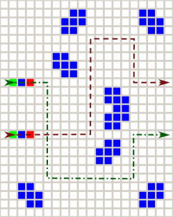
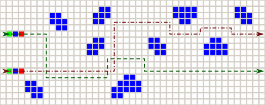
Figure 1: Swap gates: ‘wide’ (left) and ‘narrow’ (right)

Despite of relative simplicity of ‘wide’ swap, the ‘narrow’ swap may be reasonable for composition of many gates with distances between parallel signal paths equal to some fixed value, e.g. $\delta=6$.

The pictures Fig. 1 also illustrate specific way of interaction between signals and static elements: there is always an one-cell gap between them. The signal stops, because new cell may not appear near static elements and starts motion in an orthogonal direction. To prevent unlimited growth one of the directions should be limited by a design of the static elements.

The Fredkin gates together with delay elements, swaps and ‘constants’ (i.e. some amounts of auxiliary signals) allow to construct any logic circuits [16]. Necessity of some constants for used encoding is clear even from construction of NOT gate that can be expressed with Fredkin gate Eq. (6) as

$$F\!_{R}:\{A,1,0\}\to\{A,\lnot A,A\}.$$

It should be mentioned that changing direction on $90^{\circ}$ after reflection in considered RCA occupies some time (unlike BBM). For shortest signal the additional delay is one time step and points of grid critical for synchronization of arrival times should be chosen accordingly.

Similarly with BBM construction of the Fredkin gate can be expressed with simpler switch gates [16] for conditional routing of one data signal by a control one. The scheme of switch gate configuration for discussed RCA is shown on Fig. 2.

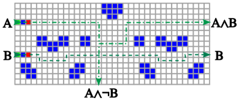
Figure 2: Signals routing and collisions in a model of switch gate

Yet another property of considered RCA is used here: after interaction between two signals with orthogonal direction and proper time delay one of them continue motion without change, but other one changes direction on $90^{\circ}$. The scheme also includes static elements necessary for direction change of data signal and delay elements to keep synchronization of two signals.

The scheme of Fredkin gate composed from four such switch gates initially proposed by R. Feynman and A. Ressler may be found in Ref. [16]. Possible realization for considered RCA is shown on Fig. 3. Without control signal two data signals follow pair of paths and simply leave the scheme with some delay, but due to interaction with control signal data signals follow other paths to exchange output positions. Many static element here is for synchronization of delays for arbitrary combinations of input signals.

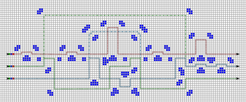
Figure 3: Signals routing and collisions in a model of Fredkin gate

Similarly with BBM the number of input and output signals for RCA $C_{0}E_{1}^{\,I\!I}$ should be equal. However, minimal modification of local rule allows to avoid such constraint. Let us save requirement about absence of occupied cells with common corner in description of local update rule of initial CEOT CA, but number of occupied cells with common edge now may be one or two. Second-order RCA produced using Eq. (5) from such rule is denoted here $C_{0}E_{1,2}^{\,I\!I}$.

Signals in modified RCA may have only minimal length (three cells). However, such kind of signals was also used in previous RCA and there is no difference with discussed examples such as switch and Fredkin gates. An essential property of new RCA is possibility to split signals. It was already mentioned, that after encountering the static obstacles signal start motion in orthogonal direction, but if both such directions are not limited by some elements, new RCA instead of stretching produces two signals moving in opposite sides.

Such property provides a counterexample to some confusion about impossibility to split signals in reversible system. The inversion of splitting element is merging of two signals. Let us consider yet another element useful for construction of Controlled-NOT gate. Similarly with switch gate it has two inputs and three output paths, but it may merge two of signals into one path. It encodes three possible non-empty combinations of two signals into one signal moving along one of three possible paths, see Fig. 4.

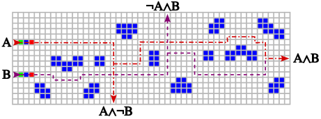
Figure 4: Transformation of two signals into three paths in RCA $C_{0}E_{1,2}^{\,I\!I}$

Controlled-NOT gate applies NOT to data signal if control signal presents

$$\{A,B\}\to\{A,A\oplus B\},$$ (7)

where $\oplus$ is addition modulo 2 (XOR). Such gate can be represented as

$$\begin{array}[]{c|c}\text{control}&\text{data}\\ \hline\cr 0&0\\ 0&1\\ 1&0\\ 1&1\\ \end{array}\to\begin{array}[]{c|c}\text{control}&\text{data}\\ \hline\cr 0&0\\ 0&1\\ 1&1\\ 1&0\\ \end{array}$$

If to consider Controlled-NOT gate as a function on pairs of bits, it exchanges rows $(1,0)$ and $(1,1)$ in the table above. It can be implemented by encoding pairs of signals into three different paths using scheme on Fig. 4, exchanging two appropriate paths and applying the inverse of the scheme (with split of signal along one of paths). Possible design is shown on Fig. 5.

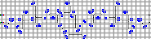
Figure 5: Signals transformations in Controlled-NOT gate for such RCA as $C_{0}E_{1,2}^{\,I\!I}$

Thus, considered family of CEOT RCA defined by property $n_{c}=0$ can be divided on two types with similar regular behavior, but with some subtleties relevant for analysis of sensitivity and reliability. The first type may use fixed number of signals with different length and for the second one the length is fixed, but signals can be split and merged.

Such a difference is mainly related with presence of pair $n_{c}=0$, $n_{e}=2$ in a sequence used for description of local rule. As examples of first type further is used already mentioned $C_{0}E_{1}^{\,I\!I}$ together with $C_{0}E_{1,3}^{\,I\!I}$ with analogue properties. The second type together with $C_{0}E_{1,2}^{\,I\!I}$ includes $C_{0}E_{1,2,3}^{\,I\!I}$ or $C_{0}E_{1-3}^{\,I\!I}$ with similar properties together with $C_{0}E_{1,2,3,4}^{\,I\!I}$ or $C_{0}E_{1-4}^{\,I\!I}$ denoted further simply as $C_{0}E_{+}^{\,I\!I}$.

The RCA $C_{0}E_{1}^{\,I\!I}$ was briefly mentioned first in Ref. [31], $C_{0}E_{1,2}^{\,I\!I}$, $C_{0}E_{+}^{\,I\!I}$ and $C_{0}E_{1-3}^{\,I\!I}$ were introduced and implemented in software developed by author with different names around the same time [32] together with yet another isotropic RCA.

Last RCA formally is not in CEOT class, but it can be considered as minimal modification of $C_{0}E_{1,2}^{\,I\!I}$ and denoted as $C_{0}E_{1,2o}^{\,I\!I}$ due to additional requirement about two non-empty neighboring cells are being opposite. Similarly with $C_{0}E_{1,2}^{\,I\!I}$ the $C_{0}E_{1,2o}^{\,I\!I}$ also may be used for gates with variable number of signals with minimal length (‘ants’).

It was already mentioned, that the second-order RCA can be considered as usual (first-order) RCA with four states. Using conversion into appropriate format for local rules with four states some numerical experiments discussed here was also performed on general software for CA simulation developed by A. Trevorrow, T. Rokicki et al [33].

3 Modelling of damage propagation

3.1 Damage propagation from single defect

Quantification of damage propagation in CA can be useful for reliability analysis of logic circuits based on such a model. Informal idea of Lyapunov exponents sometimes used as a measure of such propagation [20] and few approaches to rigorous definition are developed [34, 35, 36, 37, 38, 39] despite of certain difficulties and ambiguities related with application of such quantity to discrete systems. An intensity of defect accumulation and speed of the damage spread could be mentioned as two alternative views on the Lyapunov exponent [38].

Let us note some subtleties with definition of exponential quantities in CA. For a single defect even for an extreme case of influence on all neighbors after first step for $d$-dimensional CA there are $\epsilon=3^{d}$ affected cells in Moore neighborhood, but number of such cells grows only polynomially with time $\epsilon_{t}=(3t)^{d}$ and this amount is the maximally possible for any CA with local update rule. It provides natural constraint on exponential growth if to count defects as the total number of affected cells

$$\epsilon_{t}=O(e^{\lambda t}),\quad\lambda=\lim_{t\to\infty}\frac{1}{t}\ln\epsilon_{t}\leq\lim_{t\to\infty}\frac{1}{t}\ln(3t)^{d}=\lim_{t\to\infty}\frac{1}{t}(\ln 3+\ln t)d=0\,.$$ (8)

Such a problem could be addressed by consideration of separate replica of a system for each defect for any time step [34] with formal use of so-called Boolean derivatives [40], but such calculation without proper accounting of defects cancellation may produce overestimation of possible effects.

Let us consider 1D CA with two states and update rule

$$x_{i}^{(t+1)}=x_{i-1}^{(t)}\oplus x_{i+1}^{(t)},$$ (9)

where $\oplus$ is addition modulo 2. According to enumeration in Ref. [41] the CA corresponds to rule 90 and provides important example of additive CA [42]. Statistical properties of second-order RCA produced by such a rule denoted as 90R was discussed in Ref. [43].

For initial (irreversible) rule 90 CA calculation with Boolean derivatives produces value $\lambda=\ln 2$ for Lyapunov exponent [34]. For configuration with single occupied cell the total number of non-empty cells after $n$ steps is described by sequence A001316 in OEIS [44] and can be expressed as $2^{wt({n})}$, where $wt({n})$ is number of units in binary expansion of $n$ (Hamming weight).

Despite of exponential notation the value $2^{wt({n})}$ may not exceed $n+1$, but for any even $n$ the value doubles on next step $n+1$ resembling dynamics that could be expected for process with $\lambda=\ln 2$. Damage front for such CA moves with unit speed in both directions and could provide only minimal information for comparison with other CA [34].

Local rule for similar 2D CA with two states and von Neumann neighborhood can be expressed as

$$x_{i,j}^{(t+1)}=x_{i-1,j}^{(t)}\oplus x_{i+1,j}^{(t)}\oplus x_{i,j-1}^{(t)}\oplus x_{i,j+1}^{(t)}.$$ (10)

This CA is notable as a simple example with self-replication of any pattern discovered by E. Fredkin about 1960 and recollected by M. Gardner [25, Ch. 21]. For a single occupied cell after $n$ steps there are $4^{wt({n})}$ non-empty cells, see sequence A102376 in OEIS. For particular values of $t$ the configurations correspond to the square grids with different number of points and intervals between them. Due to Eq. (10) the CA is linear with respect to addition modulo 2 and because any pattern can be formally represented as a sum of few configurations with single occupied cell, at appropriate time steps the pattern is replicated over grids with sufficiently large intervals.

Using earlier conventions for CEOT rules such CA could be formally denoted as $C_{0-4}E_{1,3}$, but the notation $E_{1,3}$ is more natural for this CA with von Neumann neighborhood, because the local rule Eq. (10) does not depend on number of cells with common corner. The CA should be distinguished from similar replicator with Moore neighborhood [45], see sequence A160239 in OEIS.

Second-order 2D RCA from $E_{1,3}$ can be denoted as $E_{1,3}^{I\!I}$. Number of cells with different states after $n$ steps for configuration with a single cell with state 1 (red) is described by sequences A244642 and A244643 in OEIS. The RCA is not replicator, but it may produce interesting fractal-like patterns. For configuration with single red cell evolution is also coincides with considered earlier RCA $C_{0}E_{1}^{\,I\!I}$ [31] and for $C_{0}E_{1,3}^{\,I\!I}$ such coincidence also can be shown in a similar way due to some similarity of local rules with $C_{0}E_{1}^{\,I\!I}$ and $E_{1,3}^{I\!I}$, see Fig. 6.

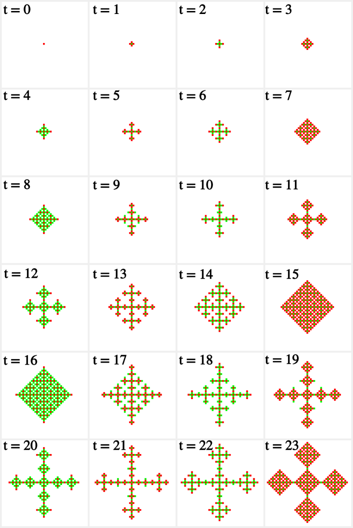
Figure 6: Evolution of red cell in $C_{0}E_{1}^{\,I\!I}$, $C_{0}E_{1,3}^{\,I\!I}$ and $E_{1,3}^{I\!I}$

The numbers $N_{1}$ and $N_{2}$ of cells with states 1 and 2 after $n$ steps for configuration with single red cell satisfy recursive formulas [31]

$$\begin{split}N_{1}(2n+1)&=4N_{1}(n),\quad N_{1}(2n+2)=N_{1}(n)+N_{1}(n+1),\\ N_{2}(2n)&=4N_{2}(n),\quad N_{2}(2n+1)=N_{2}(n)+N_{2}(n+1).\end{split}$$ (11)

The first part of each equation would correspond to asymptotically quadratic growth $O(n^{2})$, but the second part to only linear one $O(n)$. Such a variance in formal estimation of dimensions seems to be in some agreement with the shape of configurations Fig. 6 resembling some geometrical sequences used for construction of fractals [46].

Such behavior justifies consideration of models with polynomial growth together with an analogy of formal or fractal dimension [46] already investigated earlier in context of CA [18, Ch. 4] and denoted further as ${\mathfrak{D}}$ that is not vanishing unlike $\lambda$ Eq. (8)

$$\epsilon_{t}=O(t^{\mathfrak{D}}),\quad{\mathfrak{D}}(t)=\frac{\ln\epsilon_{t}}{\ln t}>0.$$ (12)

The subtleties of transition from definition of fractal dimension relevant to continuous case to such discrete systems as CA can be found in Ref [18, Ch. 4], but here formal dimension ${\mathfrak{D}}$ is treated rather as convenient quantity defined by Eq. (12).

Let us also define slightly different quantity

$${\mathfrak{D}}^{\diamond}_{t}=\frac{\ln(\epsilon_{t})}{\ln(\sqrt{2}t)}=\frac{\ln(\epsilon_{t})}{\ln(t)+\ln(2)/2}.$$ (13)

Compared to the earlier definition Eq. (12) ${\mathfrak{D}}^{\diamond}_{t}$ includes extra multiplier $\sqrt{2}$ for better adapting for diamond-like shape representing maximal possible damage spread for such kind of RCA. The number of cells for maximal possible damage is close to area of such diamond $N\simeq S=2t^{2}$ and so formal normalization for ${\mathfrak{D}}^{\diamond}=1$ should fit with $\sqrt{S}=\sqrt{2}t$, but term $\ln(2)/2\simeq 0.35$ in Eq. (13) looks relevant only for relatively small $\ln(t)$.

These parameters meet obvious inequality ${\mathfrak{D}}^{\diamond}_{t}\leq{\mathfrak{D}}_{t}$, but if the limits for $t\to\infty$ exist, they are equal and denoted further as

$${\mathfrak{D}}_{\infty}\equiv\lim_{t\to\infty}{\mathfrak{D}}_{t}=\lim_{t\to\infty}{\mathfrak{D}}^{\diamond}_{t}.$$ (14)

For $C_{0}E_{1}^{\,I\!I}$, $C_{0}E_{1,3}^{\,I\!I}$ and $E_{1,3}^{I\!I}$ for configuration with a single red cell the limit ${\mathfrak{D}}_{\infty}$ Eq. (14) does not exist, because for $\epsilon_{t}=N_{1}(t)+N_{2}(t)$ due to Eq. (11) ${\mathfrak{D}}^{\diamond}$ oscillates between ${\mathfrak{D}}^{\diamond}_{\max}=2$ and $1<{\mathfrak{D}}^{\diamond}_{\min}<2$, $\lim_{t\to\infty}{\mathfrak{D}}^{\diamond}_{\min}=1$. The Table 1 illustrates rather slow decrease of ${\mathfrak{D}}^{\diamond}_{\min}$ defined as minimal value of ${\mathfrak{D}}^{\diamond}_{t}$ for given $t$ (starting from initial value $t=1$ instead of $t=0$ used here in some illustrations).

$$\begin{array}[]{|r|r|l|}\hline\cr t&\epsilon_{t}&{\mathfrak{D}}^{\diamond}_{\min}\\ \hline\cr 2&5&1.54795206\\ 3&9&1.52037507\\ 22&181&1.51223900\\ 38&405&1.50693934\\ 42&469&1.50593450\\ 43&441&1.48232237\\ 86&1165&1.47065043\\ 171&2929&1.45445908\\ 342&7589&1.44538094\\ 683&19305&1.43576621\\ 1366&49661&1.42911275\\ 2731&126881&1.42281264\\ 5462&325525&1.41789438\\ 10923&833049&1.41343346\\ 21846&2135149&1.40970770\\ 43691&5467345&1.40636763\\ 87382&14007941&1.40346873\\ 174763&35877321&1.40086589\\ 349526&91909085&1.39855394\\ 699051&235418369&1.39646489\\ 1398102&603054709&1.39458094\\ 2796203&1544728185&1.39286577\\ 5592406&3956947021&1.39130212\\ 11184811&10135859761&1.38986817\\ 22369622&25963647845&1.38854995\\ \hline\cr\end{array}$$

Table 1: ${\mathfrak{D}}^{\diamond}_{\min}$ for $E_{1,3}^{I\!I}$ configurations starting from single red cell

The evolution of patterns from a single red cell for other RCA can be quite simple with ${\mathfrak{D}}_{\infty}=2$ for $C_{0}E_{1,2}^{\,I\!I}$ and $C_{0}E_{1-3}^{\,I\!I}$ depicted on Fig. 7 and ${\mathfrak{D}}_{\infty}=1$ for $C_{0}E_{+}^{\,I\!I}$ depicted on Fig. 8.

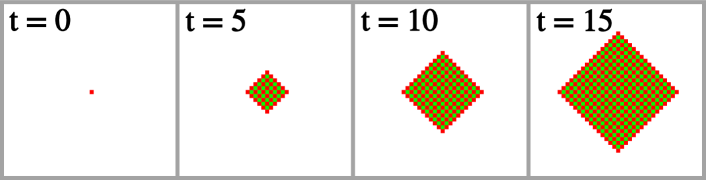
Figure 7: Evolution of red cell in $C_{0}E_{1,2}^{\,I\!I}$ and $C_{0}E_{1-3}^{\,I\!I}$

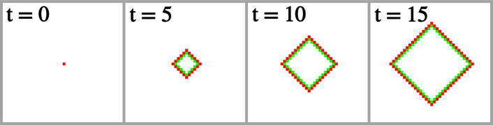
Figure 8: Evolution of red cell in $C_{0}E_{+}^{\,I\!I}$

Evolution of isotropic RCA $C_{0}E_{1,2o}^{\,I\!I}$ from single red cell is shown on Fig. 9. Analytical expression for number of cells is not known to author, but numerical estimation of ${\mathfrak{D}}^{\diamond}_{t}$ shows slow growth with minimal variations and upper limit by some value ${\mathfrak{D}}^{\diamond}_{\max}\leq 2$. For example, ${\mathfrak{D}}^{\diamond}_{\max}$ for $C_{0}E_{1,2o}^{\,I\!I}$ is increasing from ${\mathfrak{D}}^{\diamond}\simeq 1.55$ for $t=2$ to ${\mathfrak{D}}^{\diamond}\simeq 1.88$ for $t=1000$.

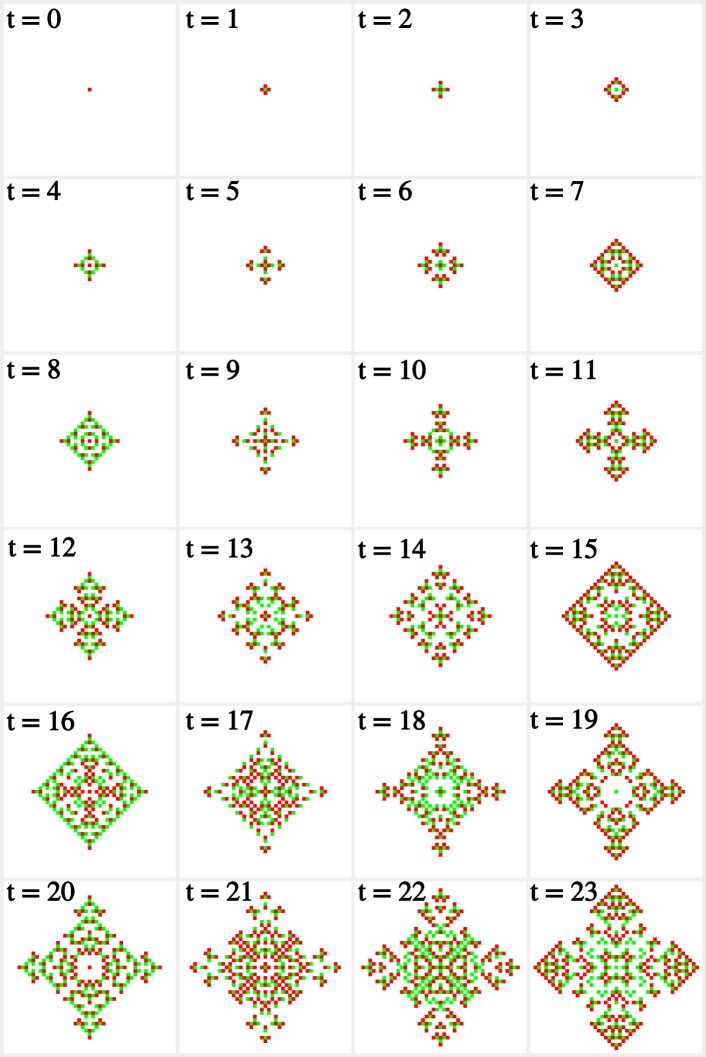
Figure 9: Evolution of red cell in $C_{0}E_{1,2o}^{\,I\!I}$

However, behavior becomes less trivial for more complex configurations. For example static $2\times 2$ blue block added to initial configuration with single red cell does not change values ${\mathfrak{D}}_{\infty}=2$ for $C_{0}E_{1,2}^{\,I\!I}$ and ${\mathfrak{D}}_{\infty}=1$ for $C_{0}E_{+}^{\,I\!I}$, but for $C_{0}E_{1-3}^{\,I\!I}$ growing rectangular area of empty cells appears inside of initial diamond patters resulting ${\mathfrak{D}}_{\infty}=1$.

Behavior looks less predictable if to add static configurations with more complex shapes. In such a case ${\mathfrak{D}}^{\diamond}$ for $C_{0}E_{+}^{\,I\!I}$ can increase from ${\mathfrak{D}}_{\infty}=1$ to ${\mathfrak{D}}_{\infty}=2$ due to many interfering damage fronts and for $C_{0}E_{1-3}^{\,I\!I}$ earlier mentioned decrease from ${\mathfrak{D}}_{\infty}=2$ to ${\mathfrak{D}}_{\infty}=1$ also can be suppressed due to similar effects. In both cases limiting value may depend in some non-trivial way from a shape of static configuration and initial position of red cell.

3.2 Damage from improper signals interaction

Despite of possible convenience for consideration of damage propagation due to certain simplification, the point-like defect discussed in Sec. 3.1 could not appear due to normal evolution of RCA. Let us consider some kind of errors due to incorrect interaction between signals such as wrong relative delays or too short intervals between consequent groups of signals.

For example, all signals should enter in a gate at the same time. A few kinds of errors could be expected due to delay between signals. The delay of output signals could be considered as a minimal possible problem. The simple example is the swap gate Fig. 1. However, even for swap gates there is critical range of delays producing more serious problems. For ‘wide’ swap gate such a critical range for delay of second (lower) signal is $3-11$ time steps and for ‘narrow’ swap the range is even bigger ($3-15$), because signal trajectories intersect repeatedly.

The similar errors can appear if interval between two consequent groups of signals is too small. For example, such delay should be at least 12 for ‘wide’ swap and 16 for ‘narrow’ swap.

Errors also may depend on particular value of delay and used RCA. Let us consider interaction of two signals approaching in orthogonal directions to the point of intersection of trajectories. The difference of distances between signals and this point can be denoted as $\Delta$. For minimal length of signals ($k=3$) some interaction occurs for $-4\leq\Delta\leq 4$. It explains value of critical range for ‘wide’ swap, because the first signal reach intersection point with additional delay 7 steps in comparison with the second one.

Collisions of signals with different delays are shown for discussed in this work RCA on Figs. 10 – 14. Due to symmetry of picture with respect to reflections about the diagonal only six values $0\leq|\Delta|\leq 5$ are shown for each case. The value $|\Delta|=5$ is the minimal one without any interaction.

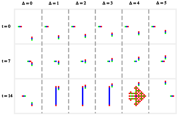
Figure 10: Collisions with different delays in $C_{0}E_{1}^{\,I\!I}$

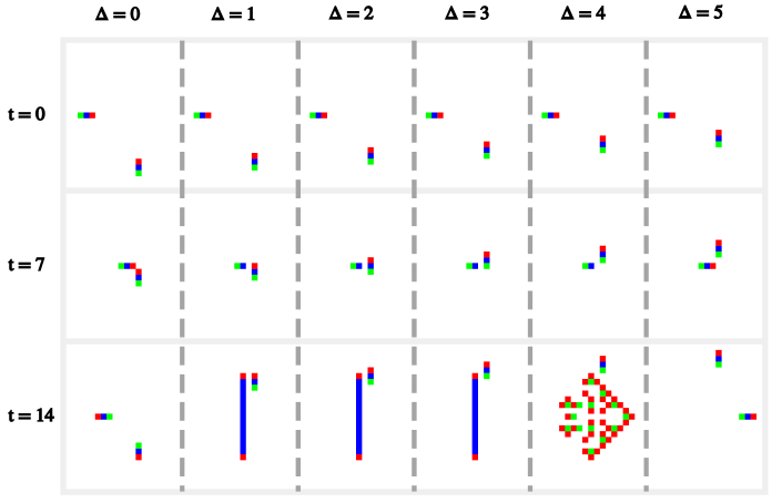
Figure 11: Collisions with different delays in $C_{0}E_{1,3}^{\,I\!I}$

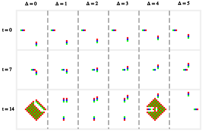
Figure 12: Collisions with different delays in $C_{0}E_{1,2}^{\,I\!I}$

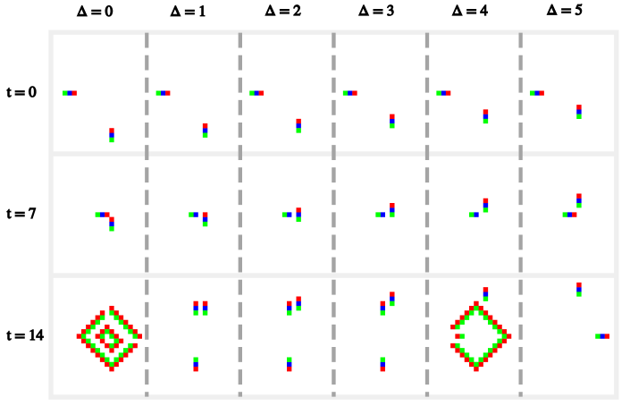
Figure 13: Collisions with different delays in $C_{0}E_{+}^{\,I\!I}$ and $C_{0}E_{1-3}^{\,I\!I}$

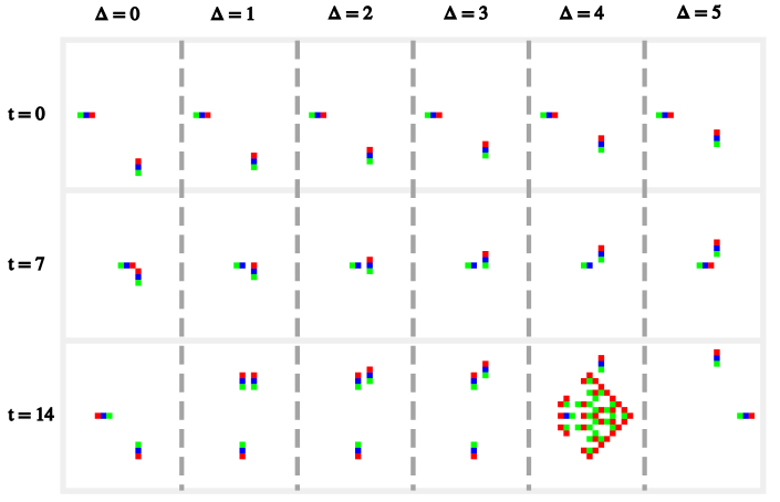
Figure 14: Collisions with different delays in $C_{0}E_{1,2o}^{\,I\!I}$

For RCA $C_{0}E_{1}^{\,I\!I}$ and $C_{0}E_{1,3}^{\,I\!I}$ of the first type sometime referred earlier as ‘snakes’ depicted on Fig. 10 and Fig. 11 the value $\Delta=0$ corresponds to reflection of signals followed by motion in opposite direction. The values $1\leq|\Delta|\leq 3$ produce a signal expanding in two opposite directions together with initial one. The value $|\Delta|=4$ seems produce more critical damage with front expanding in all possible directions.

The same value $|\Delta|=4$ also looks critical for second type of RCA $C_{0}E_{1,2}^{\,I\!I}$, $C_{0}E_{1-3}^{\,I\!I}$, $C_{0}E_{+}^{\,I\!I}$ and $C_{0}E_{1,2o}^{\,I\!I}$ sometimes referred earlier as ‘ants’ depicted on Fig. 12 – Fig. 14, but only for $C_{0}E_{1,2o}^{\,I\!I}$ value $\Delta=0$ produces simple reflection and for other four RCA of such type $\Delta=0$ causes more critical omnidirectional damage spread. The values $1\leq|\Delta|\leq 3$ for all four RCA of such type due to split of one signal after collision produce three signals moving apart with apparently smaller damage.

Both $C_{0}E_{1-3}^{\,I\!I}$ and $C_{0}E_{+}^{\,I\!I}$ produce the same damage patterns Fig. 13 with ${\mathfrak{D}}_{\infty}=2$ for $\Delta=0$ or ${\mathfrak{D}}_{\infty}=1$ for $|\Delta|=4$, despite of different behavior for initial configuration with single red cell discussed earlier, see Fig. 7 and Fig. 8.

The properties of simple collisions may only provide some guesses about behavior in more complex elements and computer simulations are necessary to clarify details. For already mentioned ‘wide’ swap the delay 7 time steps between two signals corresponds to $\Delta=0$ and produces reflection with reverse motion of signals for $C_{0}E_{1}^{\,I\!I}$, $C_{0}E_{1,3}^{\,I\!I}$ and $C_{0}E_{1,2o}^{\,I\!I}$, but for $C_{0}E_{1,2}^{\,I\!I}$, $C_{0}E_{1-3}^{\,I\!I}$ and $C_{0}E_{+}^{\,I\!I}$ the damage is more serious resembling behavior for boundary values 3 and 11 of critical range.

For ‘snakes’ $C_{0}E_{1}^{\,I\!I}$, $C_{0}E_{1,3}^{\,I\!I}$ the delay values $(4,5,6,8,9,10)$ which are not equal to ends $(3,11)$ or middle $(7)$ of critical range correspond to generation of expanding signal after collision, but interaction with static elements produces a signal with minimal length (‘ant’) and a ‘snake’ with variable length and directions depending on particular values of delay.

For all ‘ants’ $C_{0}E_{1,2}^{\,I\!I}$, $C_{0}E_{1-3}^{\,I\!I}$, $C_{0}E_{+}^{\,I\!I}$ and $C_{0}E_{1,2o}^{\,I\!I}$ collision of signals with delays $(4,5,6,8,9,10)$ produces three ‘ants’, but due to interaction after split resulting configuration includes three signals only for values $(4,6,8,9,10)$ with the particular case of delay 5 resulting omnidirectional damage front with complex shape due to interaction of two signals.

Last case also demonstrates ambiguities with characterization using formal dimensions, because even improper signal routing formally characterizing for unconstrained motion by ${\mathfrak{D}}_{\infty}\simeq 0$ may produce further a damage front with $1\leq{\mathfrak{D}}_{\infty}\leq 2$ due to interaction with static elements and other signals.

Intersection of signals in swap gates or other kinds of routing can be considered as particular problem of 2D design and resolved by analogue 3D RCA models. However for any non-trivial gate discussed above interaction of signals is necessary process. Let us consider elementary useful interaction relevant already for simple switch gate Fig. 2 to investigate errors due to wrong delays.

Such interactions are depicted on Figs. 15 – 19. The main difference in comparison with Figs. 10 – 14 is $2\times 2$ static blue block (cells with state 3) for proper signal motion after collision. The interaction between signals again corresponds to $-4\leq\Delta\leq 4$ and six values $0\leq|\Delta|\leq 5$ are enough for each case due to symmetry with respect to reflections about the diagonal.

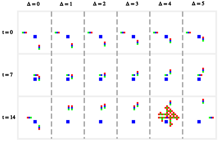
Figure 15: Interactions with different delays in $C_{0}E_{1}^{\,I\!I}$

Figure 16: Interactions with different delays in $C_{0}E_{1,3}^{\,I\!I}$

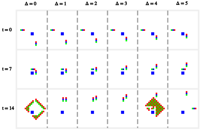
Figure 17: Interactions with different delays in $C_{0}E_{1,2}^{\,I\!I}$

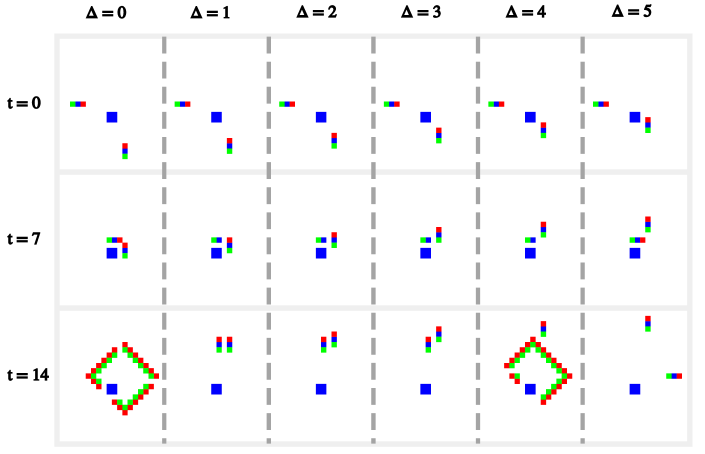
Figure 18: Interactions with different delays in $C_{0}E_{+}^{\,I\!I}$ and $C_{0}E_{1-3}^{\,I\!I}$

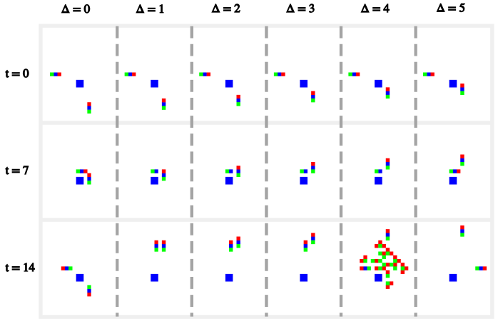
Figure 19: Interactions with different delays in $C_{0}E_{1,2o}^{\,I\!I}$

For $1\leq|\Delta|\leq 3$ after interaction two signals move along parallel paths with relative delay $|\Delta|-1$. For elements similar with switch gate Fig. 2 proper value is $|\Delta|=1$ taking into account necessity for repeated interaction. The value $|\Delta|=4$ produces omnidirectional damage front for all RCA discussed in the paper and $\Delta=0$ is related with similar problem for $C_{0}E_{1,2}^{\,I\!I}$, $C_{0}E_{1-3}^{\,I\!I}$ and $C_{0}E_{+}^{\,I\!I}$. For $C_{0}E_{1}^{\,I\!I}$, $C_{0}E_{1,3}^{\,I\!I}$ and $C_{0}E_{1,2o}^{\,I\!I}$ the same value $|\Delta|=0$ causes reflection of both signals after interaction.

Both $C_{0}E_{1-3}^{\,I\!I}$ and $C_{0}E_{+}^{\,I\!I}$ produce the same damage fronts with ${\mathfrak{D}}_{\infty}=1$, see Fig. 18. Despite of some resemblance for $\Delta=0$ of initial time steps shown on Fig. 17, ${\mathfrak{D}}_{\infty}=2$ for $C_{0}E_{1,2}^{\,I\!I}$ not only for $|\Delta|=4$, but also for $\Delta=0$ with shape of damage described as diamond-like area with rectangular empty space due to initial impact of $2\times 2$ static blue block.

3.3 Consequences of damage distribution

Description of damage distribution is also important because improper interaction of signals in some gate may produce undesirable effects on whole circuit. For ${\mathfrak{D}}_{\infty}=2$ result of such error should disrupt the proper work of other elements then it reaches them.

For ${\mathfrak{D}}_{\infty}=1$ omnidirectional damage front (see Fig. 8) also may produce the similar disruption of functionality. An alternative example of ${\mathfrak{D}}_{\infty}=1$ with anisotropic distribution can be illustrated by result of collision RCA $C_{0}E_{1}^{\,I\!I}$ or $C_{0}E_{1,3}^{\,I\!I}$ (‘snakes’) with static block. In such a case the signal starts expansion in two opposite direction. If only one of two ‘heads’ of expanding line reaches some obstacle further evolution correspond to motion of a signal in unconstrained direction.

Collision of such signal with some static element results to contraction of the signal to a size of single cell with further expansion in the perpendicular direction. Thus, interaction of single signal with static elements for $C_{0}E_{1}^{\,I\!I}$ or $C_{0}E_{1,3}^{\,I\!I}$ may finally either produce expanding line with ${\mathfrak{D}}_{\infty}=1$ or unconstrained signal motion formally resulting to ${\mathfrak{D}}_{\infty}=0$.

However, even for $C_{0}E_{1}^{\,I\!I}$ or $C_{0}E_{1,3}^{\,I\!I}$ already interaction of two signals may produce omnidirectional spreading of damage with ${\mathfrak{D}}_{\infty}=1$ or ${\mathfrak{D}}_{\infty}=2$ (see Fig. 10, Fig. 11, Fig. 15 and Fig. 16 for $|\Delta|=4$) resulting disruption of circuit functionality.

For other RCA such as $C_{0}E_{1,2}^{\,I\!I}$, $C_{0}E_{+}^{\,I\!I}$, $C_{0}E_{1-3}^{\,I\!I}$ and $C_{0}E_{1,2o}^{\,I\!I}$ (‘ants’) even for one signal collision with static block leads to the appearance of two signals moving in opposite directions. Unconstrained motion of such signals formally would result to ${\mathfrak{D}}_{\infty}=0$, but consequent collisions with static elements produce a fast increase in the number of signals. The interaction between such signals again may produce omnidirectional damage spread (see Fig. 12 – Fig. 14 and Fig. 17 – Fig. 19) generating errors in the gates affected by its propagation.

Parts of circuits can be isolated from an external damage using static elements, but such protection makes impossible an interaction between them. Signal input and output also becomes problematic with such isolation. Numerical experiments also demonstrate non-effectiveness of static elements or even movable ‘covers’ designed to protect against destructive noise between consequent signals.

Thus, for RCA considered in this work reversible circuits are very sensitive to errors. Delays of signals or too short interval between groups of signals even in one gate may result appearance of omnidirectional damage that prevents further correct operation of whole reversible logic circuits.

For example, already discussed minimum intervals between consequent signals for ‘wide’ and ‘narrow’ swap gates on Fig. 1 should be 12 and 16 time steps respectively. For Fredkin gate Fig. 3 minimum interval depends on the composition of the signal (representing combinations of zeros and units) in two consequent groups. In the worst case such interval should not be less than 22 time steps. Controlled-NOT gate on Fig. 5 can be used for RCA $C_{0}E_{1,2}^{\,I\!I}$, $C_{0}E_{+}^{\,I\!I}$, $C_{0}E_{1-3}^{\,I\!I}$ and $C_{0}E_{1,2o}^{\,I\!I}$ with a relatively short minimum possible interval of 10 time steps between consequent groups of signals.

4 Discussion and conclusions

Let us recollect properties of CA and RCA discussed in this work.

Properties $\smash{\!\!\diagdown\!\!}$ CA	$\!C_{0}E_{1}\!$	$\!C_{0}E_{1,3}\!$	$\!C_{0}E_{1,2}\!$	$\!C_{0}E_{+}\!$	$\!C_{0}E_{1-3}\!$	$\!C_{0}E_{1,2o}\!$	$\!E_{1,3}\!$
Isotropic	yes	yes	yes	yes	yes	yes	yes
CET/ET	CET	CET	CET	CET	CET	no	ET
Outer	yes	yes	yes	yes	yes	yes	yes
Linear	no	no	no	no	no	no	yes
Replicator	no	no	no	no	no	no	yes
Logic gates in second-order RCA
Swap	yes	yes	yes	yes	yes	yes
Fredkin	yes	yes	yes	yes	yes	yes
C-NOT	no	no	yes	yes	yes	yes

Property ‘outer’ emphasizes already explained in Sec. 2.2 class of ‘inner-independent’ CA. The shorter notation ET (edge-totalistic) is used instead of CET (corner-edge totalistic) for $E_{1,3}$ formally defined for von Neumann neighborhood excluding cells with common corners unlike CA with Moore neighborhood.

Despite of impossibility to use $E_{1,3}^{I\!I}$ for construction of reversible circuits this CA is included in the comparison due to known remarkable properties such as linearity and self-replication of any pattern in $E_{1,3}$ [25]. All CA used here for construction of second-order RCA could be informally treated as some non-linear modifications of the Fredkin replicator $E_{1,3}$.

The analytical formulas Eq. (11) obtained due to linearity of $E_{1,3}^{I\!I}$ also can be extended to $C_{0}E_{1}^{\,I\!I}$ [31] (and $C_{0}E_{1,3}^{\,I\!I}$) to analyse simple example of damage distribution. Oscillating behavior of formal dimension ${\mathfrak{D}}$ understandable from such expressions provides some hints about possible issues with instability in damage distribution for considered family of RCA partially confirmed by numerical experiments.

Due to such instability the RCA family has high sensitivity to errors, because even local defects or improper functionality of single gate finally leads to failure of the entire circuit. However, such behavior also provides simple error indication. A fault almost inevitably produces quickly recorded growth in total number of non-empty cells signaling a failure and preventing the completion of calculations with an incorrect result.

Similarly with BBM (billiard ball model of computations) RCA discussed in this work do not use any ‘wires’ for motion between gates. However, similar models with ‘wires’ also can be designed using generalization of second-order RCA [47] implemented in software mentioned earlier [32]. Such RCA have five states with additional one for construction of ‘wires’. That could reduce sensitivity to external noise, because all cells around wires are passive and may not participate in damage distribution. Reliability analysis for such RCA with damage distribution only along wires should be discussed elsewhere.

The existence of alternative models with ‘wires’ also justifies earlier informal name ‘wireless ants’ for part of RCA family discussed here and abbreviations for local rules such as WlAnt, WlAnt-2, WlAnt-3 and WlAnt-4 in software [32] for $C_{0}E_{1,2}^{\,I\!I}$, $C_{0}E_{+}^{\,I\!I}$, $C_{0}E_{1-3}^{\,I\!I}$ and $C_{0}E_{1,2o}^{\,I\!I}$ respectively. The local rules for $C_{0}E_{1}^{\,I\!I}$ (WlSnake) and $C_{0}E_{1,3}^{\,I\!I}$ (WlSnake-3) are implemented in the same software [32]. All rules are also converted to so-called ‘tree’ format used for CA simulations in more common software [33].

References

- [1] C.H. Bennett, Logical Reversibility of Computation, IBM J. Res. Develop. 17 (1973) 525–532.
- [2] K. Morita, Theory of Reversible Computing, Springer, New York, 2017.
- [3] I. Ulidowski, I. Lanese, U.P. Schultz, C. Ferreira (Eds.), Reversible Computation: Extending Horizons of Computing, Springer, Cham, 2020.
- [4] C. A. Mezzina, K. Podlaski (Eds.), Reversible Computing, Proc. 14th Intern. Conf. RC 2022, Springer, Cham, 2022.
- [5] M. Kutrib, U. Meyer (Eds.), Reversible Computing, Proc. 15th Intern. Conf. RC 2023, Springer, Cham, 2023.
- [6] S. Krishnaswamy, I.L. Markov and J.P. Hayes, Design, Analysis and Test of Logic Circuits Under Uncertainty, Springer, Dordrecht, 2013.
- [7] K.N. Patel, J.P. Hayes, I.L. Markov, Fault testing for reversible circuits, Proc. 21st VLSI Test Symp. (2003) 410–416; arXiv:quant-ph/0404003 (2004).
- [8] J. P. Hayes, I. Polian, B. Becker, Testing for missing-gate faults in reversible circuits, Proc. 13th Asian Test Symp. (2004) 100–105.
- [9] A.K. Singh, M. Fujita, A. Mohan (Eds.), Design and Testing of Reversible Logic, Springer, Singapore, 2020.
- [10] J. Huang, F. Lombardi, Design and Test of Digital Circuits by Quantum-Dot Cellular Automata, Artech House, Norwood, MA, 2007.
- [11] D. Kohler, J. Müller, U. Wever, Cellular probabilistic automata — A novel method for uncertainty propagation, SIAM/ASA J. Uncertain. Quantif., 2 (2014) 29–54.
- [12] S. Taati, Reversible cellular automata in presence of noise rapidly forget everything, Proc. 27th Intl. Workshop on Cellular Automata and Discrete Complex Systems (2021) 3:1–3:15; arXiv:2105.00721 (2021).
- [13] N. Margolus, Physics-like models of computation, Physica D 10 (1984) 81–95.
- [14] G.Y. Vichniac, Simulating physics with cellular automata, Physica D 10 (1984) 96–116.
- [15] T. Toffoli, N. Margolus, Invertible cellular automata: a review, Physica D 45 (1990) 229–253.
- [16] E. Fredkin, T. Toffoli, Conservative logic, Internat. J. Theor. Phys. 21 (1982) 219–253.
- [17] J. Kari, Reversible cellular automata: From fundamental classical results to recent developments, New Gener. Comput. 36 (2018) 145–172.
- [18] A. Ilachinski, Cellular Automata. A Discrete Universe, World Scientific, Singapore, 2001.
- [19] G. Rozenberg, T. Bäck, J.N. Kok (Eds.), Handbook of Natural Computing, Springer, Berlin, 2012.
- [20] S. Wolfram, Cellular automata and complexity: Collected papers, Addison-Wesley, Reading MA, 1994.
- [21] J. Kari, Theory of cellular automata: A survey, Theor. Comput. Sci. 334 (2005) 3–33.
- [22] N.H. Packard, S. Wolfram, Two-dimensional cellular automata, J. Stat. Phys. 38, (1985) 901–946.
- [23] C. Bays, A. Adamatzky (Eds.), Game of Life Cellular Automata, Springer, London, 2010.
- [24] E.R. Berlekamp, J.H. Conway, R.K. Guy, Winning Ways for Your Mathematical Plays, Vol. 4, Chap. 25, Peters, Wellesley, 2004.
- [25] M. Gardner, Wheels, Life and Other Mathematical Amusements, Freeman, San Francisco, 1983.
- [26] J.S. McCaskill, N.H. Packard, Analysing emergent dynamics of evolving computation in 2D cellular automata, in: C. Martín-Vide, G. Pond, M. A. Vega-Rodríguez (Eds.), Theory and Practice of Natural Computing, Springer, Cham, 2019, pp. 3–40.
- [27] Y. Pomeau, Invariant in cellular automata, J. Phys. A 17 (1984) L415–L418.
- [28] E. Goles, G.Y. Vichniac, Invariants in automata networks, J. Phys. A 19 (1986) L961–L965.
- [29] S. Taati, Conservation laws in cellular automata, in Ref. [19] 260–286.
- [30] G.J. Martínez. A note on elementary cellular automata classification. J. Cell. Autom. 8 (2013) 233–259; arXiv:1306.5576 (2013).
- [31] A.Y. Vlasov, On number of nonzero cells in some 2D reversible second-order cellular automata, arXiv:1407.6553 (2014).
- [32] A.Y. Vlasov, CART. Simulator of reversible and irreversible cellular automata, https://github.com/qubeat/CART (16 December 2023).
- [33] A. Trevorrow, T. Rokicki, et al, Golly 4.2. Simulator of Conway’s Game of Life and other cellular automata, https://golly.sourceforge.io (2022).
- [34] F. Bagnoli, R. Rechtman, S. Ruffo, Damage spreading and Lyapunov exponents in cellular automata, Phys. Lett. A 172 (1992) 34–38.
- [35] M.A. Shereshevsky, Lyapunov exponents for one-dimensional cellular automata, J. Nonlinear Sci. 2 (1992) 1–8.
- [36] P. Tisseur, Cellular automata and Lyapunov exponents. Nonlinearity, 13 (2000) 1547–1560.
- [37] J.M. Baetens and B. De Baets, Phenomenological study of irregular cellular automata based on Lyapunov exponents and Jacobians, Chaos 20 (2010) 033112 1–14
- [38] J.M. Baetens, J. Gravner, Introducing Lyapunov profiles of cellular automata, J. Cellular Automata 13 (2018) 267–286; arXiv:1509.06639 (2015).
- [39] On computing the Lyapunov exponents of reversible cellular automata, Natural Computing 20 (2021) 273–286.
- [40] G.Y. Vichniac, Boolean derivatives on cellular automata, Physica D 45 (1990) 63–74.
- [41] S. Wolfram, Statistical mechanics of cellular automata, Rev. Mod. Phys. 55 (1983), 601–644.
- [42] O. Martin, A.M. Odlyzko, S. Wolfram, Algebraic properties of cellular automata, Commun. Math. Phys. 93 (1984) 219–258.
- [43] S. Takesue, Reversible cellular automata and statistical mechanics, Phys. Rev. Lett. 59 (1987) 2499–2502.
- [44] OEIS Foundation Inc. (2023), The On-Line Encyclopedia of Integer Sequences, published electronically at https://oeis.org.
- [45] N.J.A. Sloane, On the number of ON cells in cellular automata, in: S. Butler, J. Cooper, G. Hurlbert (Eds.), Connections in Discrete Mathematics, CUP, Cambridge, 2018, pp. 13–38; arXiv: 1503.01168 (2015).
- [46] T. Vicsec, Fractal Growth Phenomena, World Scientific, Singapore, 1999.
- [47] A.Y. Vlasov, On generalization of reversible second-order cellular automata, arXiv:1311.4297 (2013).