Order-by-disorder in the antiferromagnetic long-range transverse-field Ising model on the ruby lattice

Abstract

We demonstrate that geometric frustration and long-range interactions both promote order-by-disorder in the antiferromagnetic transverse-field Ising model on the ruby lattice. To this end we investigate the quantum phase diagram for truncated $J_{1}$-$J_{2}$-$J_{3}$ Ising interactions. In the low-field limit we derive an effective quantum dimer model, analyzing how the extensive ground-state degeneracy at zero field is lifted by two distinct order-by-disorder scenarios. We support our analysis by studying the gap-closing of the high-field phase using series expansions. For $J_{2}>J_{3}$, we find an emergent clock-ordered phase at low fields, stabilized by resonating plaquettes, and a 3d-XY quantum phase transition to the polarized high-field phase. For $J_{3}>J_{2}$, an order-by-disorder mechanism stabilizes a distinct $\bm{k}=(0,0)$ order and a quantum phase transition in the 3d-Ising universality class is observed. In contrast to the triangular lattice, on the ruby lattice algebraically decaying long-range interactions favor the clock-ordered low-field phase and therefore allow a robust implementation in existing Rydberg atom quantum simulators.

Extensively degenerate ground-state spaces due to frustration pose a formidable resource for emergent exotic quantum phenomena. Frustration arises either from conflicting spin interactions like, most prominently, in Kitaev’s honeycomb model [1] or due to the lattice geometry like in antiferromagnetic quantum magnets on the triangular [2, 3, 4, 5, 6, 7], Kagome [8, 4, 5, 9, 7], or pyrochlore [10, 11] lattice containing loops of odd length. Perturbing extensively degenerate ground-state spaces may result in several distinct scenarios. First, a distinct symmetry-broken order can emerge for infinitesimal perturbations (order-by-disorder) [12, 4, 5, 6, 7]. Second, a direct realization of a symmetry unbroken phase may occur (disorder-by-disorder). This phase can either be trivial [8, 13, 7] or exotic like the occurrence of quantum spin liquids [14, 15, 16, 10, 11, 17].

A distinct strand of recent research focuses on quantum phenomena in many-body systems with long-range interactions [18]. Such systems are relevant for a wide range of quantum-optical platforms including cold atoms [19, 20, 21] and ions [22, 23, 24, 25, 26, 27, 28, 29, 30]. In particular, Rydberg atom quantum simulators are a promising platform to study frustrated Ising quantum spin systems with long-range interactions [31, 32, 33, 34, 35, 36, 20, 37, 38]. Recent theoretical [39, 40] and experimental [38] studies of Rydberg atoms on the Ruby lattice demonstrate a rich quantum phase diagram including a $\mathbb{Z}_{2}$ quantum spin liquid [39, 38]. Further, unfrustrated quantum systems with long-range interactions are known to display exotic quantum-critical properties like continuously varying critical exponents [41, 42, 43, 44, 45, 46, 47, 48, 49, 50]. In contrast, geometric frustration and long-range interactions typically compete with each other, i. e., quantum fluctuations favor different ground states compared to the ones that benefit from the long-range interactions [51]. An important example is the clock-ordered phase in the nearest-neighbor transverse-field Ising model (TFIM) on the triangular lattice resulting from an order-by-disorder scenario at low fields, which is destroyed by long-range Ising interactions giving rise to a stripe phase [52, 53, 54, 44, 55, 51].

In this communication we demonstrate for the antiferromagnetic TFIM on the ruby lattice that the geometric frustration and long-range interactions promote the same order-by-disorder mechanism. The truncated $J_{1}$-$J_{2}$-$J_{3}$ interactions result in an extensively degenerate ground-state space due to geometric frustration in the absence of a field. We study the breakdown of this degeneracy in the presence of a small field by deriving the leading order effective Hamiltonians in two limiting cases. First, we consider the $J_{1}$-$J_{2}$ case, where we derive a low-field description analogous to the paradigmatic dual-dimer model describing the low-field behavior of the nearest-neighbor TFIM on the triangular lattice [4, 5, 6]. We demonstrate the existence of an emergent clock-ordered low-field phase resulting from an order-by-disorder scenario and the corresponding 3d-XY quantum phase transition to the high-field phase from high-field series expansions [56, 57, 7, 58]. Second, we repeat our investigations along the same lines for the $J_{1}$-$J_{3}$ case and find a diagonal effective low-field Hamiltonian resulting in an order-by-disorder scenario to a gapped $\bm{k}=(0,0)$ order with a 3d-Ising quantum phase transition to the high-field phase. Further, we infer the phase diagram for the general $J_{1}$-$J_{2}$-$J_{3}$ model from the two previously considered limiting cases. Most importantly, we find that the full algebraically decaying long-range Ising interaction favors also the clock-ordered phase and therefore allows a robust implementation in existing Rydberg atom simulators.

Model.– We approach our study of the antiferromagnetic long-range TFIM on the ruby lattice by first focusing on the general $J_{1}$-$J_{2}$-$J_{3}$ TFIM which contains the case of truncated long-range interactions decaying with $|\bm{i}-\bm{j}|^{-\alpha}$. The Hamiltonian is given by

$$\mathcal{H}=J_{1}\sum_{\langle i,j\rangle_{1}}\sigma_{i}^{z}\sigma_{j}^{z}+J_{2}\sum_{\langle i,j\rangle_{2}}\sigma_{i}^{z}\sigma_{j}^{z}+J_{3}\sum_{\langle i,j\rangle_{3}}\sigma_{i}^{z}\sigma_{j}^{z}+h\sum_{i}\sigma_{i}^{x}$$ (1)

with Pauli matrices $\sigma_{i}^{x/z}$ describing spins-$1/2$ located on lattice sites $i$. The three couplings $J_{1},J_{2},J_{3}\geq 0$ define the interaction strengths between sites as depicted in Fig. 1, such that the coupling $J_{1}\geq 0$ denotes interactions between nearest-neighbor sites, while $J_{2}\geq 0$ and $J_{3}\geq 0$ denote interactions between the second- and third-nearest-neighbor sites for all aspect ratios $\rho=r_{2}/r_{1}>1$ (see Fig. 1). The transverse-field amplitude is denoted by $h$. For $h\gg J$ the ground state of the model is a trivial $x$-polarized phase.

The ruby lattice can be understood as a triangular lattice with elementary lattice vectors $\bm{t}_{1}$ and $\bm{t}_{2}$ and six sites per unit cell at positions $\bm{\delta}_{1},\ldots,\bm{\delta}_{6}$ (compare Fig. 1). We set the distance between sites interacting via $J_{1}$ to $r_{1}=1$. We note that the aspect ratio $\rho=\sqrt{3}$ chosen for all illustrations corresponds to placing the atoms on the links of a Kagome lattice.

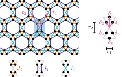
Figure 1: Illustration of the ruby lattice with $\rho=r_{2}/r_{1}=\sqrt{3}$, showing the geometry of the three nearest-neighbor couplings $J_{1}$, $J_{2}$ and $J_{3}$, the elementary lattice vectors $\bm{t}_{1}$ and $\bm{t}_{2}$ and the positions $\bm{\delta}_{1},\ldots,\bm{\delta}_{6}$ of the six sites in the unit cell. For this aspect ratio, the geometry of the ruby lattice is equivalent to placing atoms on the links of a Kagome lattice.

In the limiting cases of two vanishing couplings $J_{i}$ the ruby lattice decomposes into isolated structures. For $J_{2}=J_{3}=0$ the lattice reduces to isolated triangles, for $J_{1}=J_{3}=0$ to isolated hexagons and for $J_{1}=J_{2}=0$ to decoupled chains. As long as $J_{1}>0$ the system is geometrically frustrated and there is an extensive number of ground states for $h=0$.

$J_{1}$-$J_{2}$ case.- The subsequent low-field analysis of the case $J_{1},J_{2}>0$ and $J_{3}=0$ is independent of the ratio $J_{2}/J_{1}$.

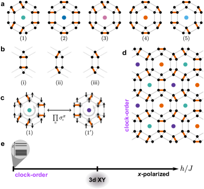
Figure 2: $J_{1}$-$J_{2}$ model. (a) Illustration of hexagonal plaquettes minimizing the number of frustrated ferromagnetic $J_{1}$-bonds (orange; antiferromagnetic bonds in gray). (b) Unit-cell configurations appearing within the zero-field ground states. (c) Leading sixth-order off-diagonal process inducing resonances between type-(1) and -($1^{\prime}$) plaquettes. (d) Emerging $\bm{k}=(2\pi/3,-2\pi/3)$ clock-ordered ground-state in the low-field limit. (e) Sketch of the quantum phase diagram: The extensive degeneracy of the zero-field ground state breaks town to a clock order in an order-by-disorder scenario for infinitesimal transverse fields, followed by a 3d-XY phase transition into the trivial $x$-polarized phase.

Ground states at $h=0$ minimize the number of frustrated ferromagnetic $J_{1}$-bonds. All these states contain only hexagonal plaquettes of the five types represented (up to rotations) in Fig. 2a. The resulting zero-field ground-state manifold is extensively degenerate. Note that in all those states, no $J_{2}$ bond is ferromagnetic and thus the ground-state manifold is independent from the ratio $J_{1}/J_{2}$. We analyze the leading-order low-field contributions by performing degenerate perturbation theory around $h=0$, including both diagonal and off-diagonal processes [59] (see supplemental material in Ref. [60]). We find that the leading-order contribution lifting the ground-state degeneracy is a fourth-order diagonal energy correction selecting type-(1) and type-(4) plaquettes. For this we evaluate the diagonal energy corrections on the three unit cell configurations of the zero-field ground-state plaquettes, depicted in Fig. 2b. The energy corrections in fourth order yield the decreasing energetic hierarchy of the unit cells as $(\mathrm{i})\to(\mathrm{ii})\to(\mathrm{iii})$ for $J_{1},J_{2}>0$. As each plaquette implies the same density of 1/3 unit cells (i) on the lattice, plaquettes (1) and (4) are beneficial as they contain zero unit cells (iii).

To understand the emerging low-field phase we construct the zero-field states containing exclusively type-(1) and (4) plaquettes, resulting in a $\sqrt{3}\times\sqrt{3}$ clock-ordered structure on the triangular lattice on which the plaquettes are arranged as depicted in Fig. 2d. Respective states are selected from the extensively degenerate ground-state manifold in an order-by-disorder scenario for $h>0$. We further find that the leading-order off-diagonal contribution is a resonant sixth-order process acting on the inner sites of the hexagon of plaquettes of type-(1) mapping them to type-(1^′) plaquettes (see Fig. 2c). The density of type-(1) and type-(1^′) plaquettes is maximized by the subspace of $\sqrt{3}\times\sqrt{3}$ clock-ordered structures already selected by the diagonal fourth-order corrections. The action of the transverse field on respective states in sixth order is analogous to the one in first order within the antiferromagnetic TFIM on the triangular lattice [4, 5, 6, 55]. In analogy to the effective quantum-dimer model in the low-field limit on the triangular lattice [61, 4, 5, 6], we describe the low-field limit on the ruby lattice as

$$\mathcal{H}_{\mathrm{eff}} =\bar{E}_{0}+\frac{h^{4}}{2}\sum_{\hskip 1.42271pt\includegraphics[height=8.0pt,valign={c}]{symbol7.pdf}\hskip 1.42271pt}\quad\sum_{\mathclap{\begin{subarray}{c}\leavevmode\hbox to5.69pt{\vbox to5.69pt{\text{[drawing]}}}=\leavevmode\hbox to5.69pt{\vbox to5.69pt{\text{[drawing]}}},\leavevmode\hbox to5.69pt{\vbox to5.69pt{\text{[drawing]}}},\leavevmode\hbox to5.69pt{\vbox to5.69pt{\text{[drawing]}}},\\ \quad\leavevmode\hbox to5.69pt{\vbox to5.69pt{\text{[drawing]}}},\leavevmode\hbox to5.69pt{\vbox to5.69pt{\text{[drawing]}}}\end{subarray}}}\quad\left(E_{J_{2}}^{(4)}({\leavevmode\hbox{$\vbox{\hbox{\resizebox{}{}{{\leavevmode\hbox{\set@color{ \leavevmode\hbox to5.69pt{\vbox to5.69pt{\text{[drawing]}}}}}}}}}$}})\ket{\hskip 1.42271pt\includegraphics[height=20.0pt,valign={c}]{symbol8.pdf}\hskip 1.42271pt}\bra{\hskip 1.42271pt\includegraphics[height=20.0pt,valign={c}]{symbol8.pdf}\hskip 1.42271pt}\right)+$$

$$+h^{6}\sum_{\hskip 1.42271pt\includegraphics[height=8.0pt,valign={c}]{symbol7.pdf}\hskip 1.42271pt}E_{\mathrm{res}}^{(6)}\left(\ket{\hskip 1.42271pt\includegraphics[height=20.0pt,valign={c}]{symbol1.pdf}\hskip 1.42271pt}\bra{\hskip 1.42271pt\includegraphics[height=20.0pt,valign={c}]{symbol2.pdf}\hskip 1.42271pt}+\mathrm{h.c.}\right)\,,$$ (2)

where the sum runs over all plaquettes within the lattice and $\bar{E}_{0}$ is a constant containing perturbative contributions which are equal for all ground states. For the sake of a compact notation, the first sum containing the diagonal terms runs over all five plaquette types defined in Fig. 2a (up to rotations). The diagonal corrections $E_{J_{2}}^{(4)}({\leavevmode\hbox{$\vbox{\hbox{\resizebox{}{}{{\leavevmode\hbox{\set@color{ \leavevmode\hbox to5.69pt{\vbox to5.69pt{\text{[drawing]}}}}}}}}}$}})$ of the five plaquette types and the amplitude of the resonating process $E_{\mathrm{res}}^{(6)}$ are given in Ref. [60].

Motivated by the analogous low-field description of the two models, one expects a 3d-XY quantum phase transition from the clock-ordered phase towards the $x$-polarized high-field phase [61, 4, 5, 6]. We confirm this scenario by high-field series expansions using the method of perturbative continuous unitary transformations (pCUT) [56] with the help of linked-cluster expansions set up as a full graph decomposition [62, 58, 63, 64] and DlogPadé extrapolations [65, 66] (for details see Ref. [60]) to investigate the closing of the elementary excitation gap. We determine the series of the gap up to order 10 for the general $J_{1}$-$J_{2}$ case and order 11 for $J_{1}=J_{2}$. With this analysis we determine the critical momentum $\bm{k}$, critical point $\lambda_{c}$, and gap exponent $z\nu$ of a potential quantum phase transition. We find the critical gap momentum at ${\bm{k}=(2\pi/3,-2\pi/3)}$ reflecting the periodicity of the $\sqrt{3}\times\sqrt{3}$ structure and a closing of the excitation gap at some critical point $\lambda_{c}$ for all ratios of $J_{1}/J_{2}$ except for $J_{1}/J_{2}\rightarrow\infty\,(J_{1}/J_{2}\to 0)$ approaches the limit of decoupled triangles (hexagons), where $\lambda_{c}$ shifts towards large coupling strengths. The associated critical exponents $z\nu$, e. g., $z\nu=0.806\pm 0.056$ for the case $J_{1}=J_{2}$, are in line with the conjectured 3d-XY universality class with $z=1$ and $\nu_{\mathrm{3d-XY}}=0.67169(7)$ [67, 68] within the limitations of the series expansion. The latter is known to slightly overestimate critical exponents and especially the determination of 3d-XY exponents is challenging [7, 44]. In comparison to the triangular lattice the considered perturbative processes span even fewer unit cells on the ruby lattice so that a larger deviation to the known critical exponents is reasonable. The critical point as well as the gap exponent as a function of $J_{1}/J_{2}$ are depicted in Ref. [60].

$J_{1}$-$J_{3}$ case.- Next we consider the case $J_{1},J_{3}>0$ and $J_{2}=0$. Again, the low-field scenario is independent of the ratio $J_{1}/J_{3}$.

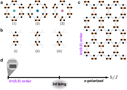
Figure 3: $J_{1}$-$J_{3}$ model. (a) Illustration of hexagonal plaquettes minimizing the number of frustrated ferromagnetic $J_{1}$-bonds (orange). Antiferromagnetic bonds drawn in gray. (b) Unit-cell configurations appearing within the zero-field ground states. (c) Emerging $\bm{k}=(0,0)$ ordered ground-state in the low-field limit. (d) Sketch of the quantum phase diagram: The extensive degeneracy of the zero-field ground state breaks town to a $\bm{k}=(0,0)$ order in an order-by-disorder scenario for infinitesimal transverse fields, followed by a 3d-Ising phase transition into the trivial $x$-polarized phase.

At $h=0$, ground states contain only hexagonal plaquettes of the three types depicted in Fig. 3a, each type including all plaquettes related to the one depicted by rotation. The manifold of ground states build from these three plaquette types is extensively degenerate. Since there is no ferromagnetic $J_{3}$ bond in a zero-field ground state, the zero-field results are independent of $J_{3}$. We investigate the low-field limit by performing degenerate perturbation theory around $h=0$. We demonstrate that the leading-order contribution lifting the ground-state degeneracy is a fourth-order process by evaluating the diagonal energy corrections for all zero-field ground states analogous to the $J_{1}$-$J_{2}$ case. We find the decreasing energetic hierarchy of the unit cells depicted in Fig. 3b as $(\mathrm{i})\to(\mathrm{iii})\to(\mathrm{ii})$. In fact, there can be no finite-order off-diagonal process in the $J_{1}$-$J_{3}$ case: When performing a spin flip within a zero-field ground state, one introduces two domain walls in the $J_{3}$ chain the affected site is part of. Therefore, to map one zero-field ground state to another, one needs to flip at least all spins along the $J_{3}$ chain. The effective Hamiltonian in the low-field limit reads

$$\mathcal{H}_{\mathrm{eff}} =\bar{E}_{0}+h^{4}\sum_{\hskip 1.42271pt\includegraphics[angle={90},height=5.0pt,valign={c}]{symbol12.pdf}\hskip 1.42271pt}\left(E_{J_{3}}^{(4)}(\mathrm{i})\ket{\hskip 1.42271pt\includegraphics[angle={90},height=8.0pt,valign={c}]{symbol9.pdf}\hskip 1.42271pt}\bra{\hskip 1.42271pt\includegraphics[angle={90},height=8.0pt,valign={c}]{symbol9.pdf}\hskip 1.42271pt}+\right.$$ (3)

$$+ \left.E_{J_{3}}^{(4)}(\mathrm{ii})\ket{\hskip 1.42271pt\includegraphics[angle={90},height=8.0pt,valign={c}]{symbol10.pdf}\hskip 1.42271pt}\bra{\hskip 1.42271pt\includegraphics[angle={90},height=8.0pt,valign={c}]{symbol10.pdf}\hskip 1.42271pt}+E_{J_{3}}^{(4)}(\mathrm{iii})\ket{\hskip 1.42271pt\includegraphics[angle={90},height=8.0pt,valign={c}]{symbol11.pdf}\hskip 1.42271pt}\bra{\hskip 1.42271pt\includegraphics[angle={90},height=8.0pt,valign={c}]{symbol11.pdf}\hskip 1.42271pt}\right)\,,$$

where $\bar{E}_{0}$ is a constant containing perturbative contributions which are equal for all ground states. The amplitudes $E_{J_{3}}^{(4)}(\mathrm{i,ii,iii})$ are listed in Ref. [60]. As each zero-field plaquette implies the same density of 1/3 unit cells (i) on the lattice, we derive the ground-state configuration for $h>0$ by maximizing the density of the energetically second-most beneficial unit cell (iii) and thus plaquette of type-(1) (see Fig. 3c). We find a diagonal order-by-disorder scenario where the quantum fluctuations stabilize a $\bm{k}=(0,0)$ state adiabatically connected to the order presented in Fig. 3 for all $J_{1},J_{3}>0$. From this low-field scenario a 3d-Ising quantum phase transition to the $x$-polarized high-field phase is expected and we confirm this with the subsequent high-field analysis analogous to the $J_{1}$-$J_{2}$ case. We determine the series of the gap up to order 10 for the general $J_{1}$-$J_{3}$ case and order 11 for $J_{1}=J_{3}$.

The critical gap momentum $\bm{k}=(0,0)$ found in series expansions around the high-field limit for all ratios $J_{1}/J_{3}$ verifies the low-field order. We find a quantum phase transition for all $J_{1}/J_{3}>0$. Similar to the $J_{1}$-$J_{2}$ case, $\lambda_{c}$ shifts to large couplings for $J_{1}/J_{3}\rightarrow\infty$, while $\lambda_{c}\to 0.5$ as the limit of isolated chains is approached for $J_{1}/J_{3}\rightarrow 0$. By investigating the critical exponent $z\nu$, we demonstrate the expected 3d-Ising where $\nu_{\text{3d-Ising}}=0.629971(4)$ [69], e. g., we find $z\nu=0.632\pm 0.101$ for $J_{1}=J_{3}$. The critical point and exponent as a function of $J_{1}/J_{3}$ are depicted in Ref. [60]. Note that the extracted gap exponent is more accurate compared to the 3d-XY exponent in the $J_{1}$-$J_{2}$ model.

$J_{1}$-$J_{2}$-$J_{3}$ case.- We continue by deriving the $J_{1}$-$J_{2}$-$J_{3}$ phase diagram from the two limiting cases considered so far. We define $J_{2}=\cos\theta\,J_{1}$ and $J_{3}=\sin\theta\,J_{1}$. The zero-field ground states of the $J_{1}$-$J_{2}$ case and the $J_{1}$-$J_{3}$ case have the two distinct energies $\frac{1}{3}J_{1}+\frac{2}{3}J_{3}$ and $\frac{1}{3}J_{1}+\frac{2}{3}J_{2}$ per site in the full $J_{1}$-$J_{2}$-$J_{3}$ model for $h=0$. Thus, for $J_{2}>J_{3}$ ($J_{3}>J_{2}$) the $J_{1}$-$J_{2}$ ($J_{1}$-$J_{3}$) ground states have a lower energy than the $J_{1}$-$J_{3}$ ($J_{1}$-$J_{2}$) ground states and realize ground states of the $J_{1}$-$J_{2}$-$J_{3}$ model. From the preceding low-field analysis we argue that for all $J_{2}>J_{3}$ an order-by-disorder mechanism to a clock order must be present as the $J_{1}$-$J_{2}$ ground states also realize the zero-field ground states here. Following the same argument, an order-by-disorder to the $\bm{k}=(0,0)$ ordered state takes place for all $J_{3}>J_{2}$.

The orders found by the low-field analysis are stable until the point $\lambda_{c}$ where a quantum phase transition towards the high-field phase takes place. Using series expansions as before, the critical gap momenta correspond indeed to the expected momenta ${\bm{k}=(2\pi/3,-2\pi/3)}$ for $J_{2}>J_{3}$ and $\bm{k}=(0,0)$ for $J_{3}>J_{2}$.

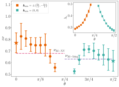
Figure 4: Critical point $\lambda_{c}$ (inset) and gap exponent $z\nu$ in the $J_{1}$-$J_{2}$-$J_{3}$ TFIM from high-field series expansions tuning with $\theta$ from the $J_{1}$-$J_{2}$ to the $J_{1}$-$J_{3}$ case. The critical exponents match the two expected exhibit two universality classes 3d-XY for $J_{2}>J_{3}$ and 3d-Ising for $J_{3}>J_{2}$ with an accuracy similar to the results in the limiting cases $J_{1}$-$J_{2}$ to the $J_{1}$-$J_{3}$ which are marked by the respective stars. The depicted results resemble averages over several high-order extrapolants with the respective standard deviation.

We extract the critical exponent $z\nu$ from the gap-closing at $\lambda_{c}$ as shown in Fig. 4 as a function of $\theta$, i. e., sweeping from the $J_{1}$-$J_{2}$ to the $J_{1}$-$J_{3}$ case. We calculate the series expansion of the gap up to order 9 for the general $J_{1}$-$J_{2}$-$J_{3}$ case. We find a divergence of $\lambda_{c}$ approaching the symmetric $J_{2}=J_{3}$ case at $\theta=\pi/4$ from both sides. Regarding the gap exponent $z\nu$ we find a qualitative match with the expected quantum criticalities (3d-XY criticality for $J_{2}>J_{3}$ and 3d-Ising criticality for $J_{3}>J_{2}$). The agreements with the respective literature values are comparable to the ones in the two previously analyzed limiting $J_{1}$-$J_{2}$ and $J_{1}$-$J_{3}$ cases. In particular, as discussed for the $J_{1}$-$J_{2}$ case, the DlogPadé approximants systematically overestimate the critical exponent for $J_{2}>J_{3}$. As $\lambda_{c}$ shifts to infinity for $J_{2}\approx J_{3}$, the estimation of the critical exponent becomes unreliable.

Indeed, the point $J_{2}=J_{3}$ is special in the $J_{1}$-$J_{2}$-$J_{3}$ TFIM. At ${h=0}$, the degeneracy of $J_{1}$-$J_{2}$ and $J_{1}$-$J_{3}$ ground states is further enhanced by multiple additional ground states [60]. Further, the extrapolation of the high-field gap located at $\bm{k}=(2\pi/3,-2\pi/3)$ does not indicate any gap-closing. One therefore may speculate about a disorder-by-disorder scenario so that the ground state at infinitesimally small $h$ is adiabatically connected to the high-field limit [7]. Note that proving a disorder-by-disorder scenario using solely series expansion methods is not possible and further investigations using other methods are necessary [7].

Altogether, we have shown that the general $J_{1}$-$J_{2}$-$J_{3}$ TFIM features a plethora of intriguing ground-state phenomena including two distinct order-by-disorder mechanisms.

Experimental realization.- The so far considered model contains a truncated version of the TFIM with algebraically decaying long-range interactions. Here we show how Rydberg atom quantum simulators [20] can implement the order-by-disorder scenario to the clock-ordered phase of the TFIM on the ruby lattice even in the presence of long-range interactions. The physics of Rydberg atom arrays can be modeled with the two-dimensional Fendley-Sengupta-Sachdev model [34, 39]

$$\mathcal{H}^{\mathrm{FSS}}=\frac{\Omega}{2}\sum_{i}\left(b_{i}^{\phantom{\dagger}}+b_{i}^{\dagger}\right)-\delta\sum_{i}n_{i}\ +\sum_{i<j}\frac{C_{6}}{|\bm{i}-\bm{j}|^{6}}n_{i}n_{j}$$ (4)

with hardcore bosonic operators $b_{i}^{\dagger}=\ket{e}_{i}\bra{g}_{i}$ (${b_{i}^{\phantom{\dagger}}=\ket{g}_{i}\bra{e}_{i}}$) (de)exciting a Rydberg atom and ${n_{i}=b_{i}^{\dagger}b_{i}^{\phantom{\dagger}}}$ counting the excitations at site $i$. Excited Rydberg atoms interact via an algebraically decaying long-range van-der-Waals interaction $\sim|\bm{i}-\bm{j}|^{-6}$ with van-der-Waals coefficient $C_{6}$. Identifying the Pauli matrices $\sigma_{i}^{x}=b_{i}^{\phantom{\dagger}}+b_{i}^{\dagger}$ and $\sigma_{i}^{z}=1-2n_{i}$, we arrive up to a constant at the spin Hamiltonian

$$\mathcal{H}^{\mathrm{FSS}}=h\sum_{i}\sigma_{i}^{x}+\left(\frac{\delta}{2}-\frac{C_{6}\mu}{4}\right)\sum_{i}\sigma_{i}^{z}+\frac{1}{4}\sum_{i<j}\frac{C_{6}}{|\bm{i}-\bm{j}|^{6}}\sigma_{i}^{z}\sigma_{j}^{z}$$ (5)

with $\mu=\sum_{\bm{d}}|\bm{d}|^{-6}$, summing over all vectors $\bm{d}$ between interacting sites on the lattice, and $h=\Omega/2$. To recover the TFIM, the longitudinal field must be zero, yielding the condition $\delta=C_{6}\mu/2$ for the laser detuning. As the algebraically decaying interaction strength implies $J_{1}\geq J_{2}>J_{3}$ for $\rho\geq 1$, from our previous analysis of the $J_{1}$-$J_{2}$-$J_{3}$ TFIM we expect an order-by-disorder mechanism into a clock-ordered phase upon tuning the Rabi frequency $\Omega$ from zero to a finite value and a 3d-XY quantum phase transition into the polarized phase. The case of $J_{3}\geq J_{2}$ can not be realized on such a platform.

The ruby lattice with aspect ratio $\rho=\sqrt{3}$ is equivalent to placing sites on the links of a Kagome lattice. In a recent work [38], Rydberg atoms on such a geometry were used to probe topological spin liquids in agreement with theoretical studies [39, 40]. From this geometry we obtain $J_{1}=C_{6}/4$, $J_{2}=J_{1}/27$, $J_{3}=J_{1}/64$, truncating all $J_{i}\leq J_{4}=J_{1}/343$ for the series expansion. In this case the $J_{1}$ interactions dominate ($J_{1}\gg J_{2}>J_{3}$) and the system consists of almost isolated triangles, resulting in an almost flat dispersion and no closing of the excitation gap at momentum $\bm{k}=(2\pi/3,-2\pi/3)$ can be detected within the perturbative series expansion (see supplemental material in Ref. [60]).

Decreasing the aspect ratio $\rho$, which is a free tuning parameter in the experiment, decreases the ratio of $J_{1}/J_{2}$. Setting e. g. $\rho=1$, we have $J_{1}=J_{2}$ and $J_{3}=J_{1}/8$, again neglecting all $J_{i}\leq J_{4}=J_{1}/27$. From pCUT calculations we predict a quantum phase transition at $C_{6}/\Omega\approx 1.202\pm 0.012$ from the clock-ordered phase towards the trivial polarized phase. The associated critical exponent $z\nu=0.801\pm 0.046$ is in line with the predicted 3d-XY criticality within previously discussed limitations.

We further demonstrate the order-by-disorder mechanism in the presence of the full algebraically decaying long-range interaction taking into account $J_{i}\leq J_{4}$. Following the approach described in Ref. [51] we search for the energetically most beneficial configuration in the limit of $h=0$, taking into account the entire, untruncated long-range interactions via resummed couplings. Coming from the degenerate zero-field ground state in the $J_{1}$-$J_{2}$-$J_{3}$ TFIM, we find that the same clock-ordered states are selected by both: the long-range interaction and an infinitesimal transverse field. This is remarkable as in other well-known order-by-disorder scenarios, e. g., for the antiferromagnetic TFIM on the triangular lattice, the long-range interactions compete with the fluctuations induced by the transverse field [52, 53, 54, 44, 55, 51].

Conclusions.- In this communication we showed for the low-field limit of the TFIM on the ruby lattice that long-range interactions and geometric frustration do not compete for different ground states but promote the same one. In particular, the quantum fluctuations induce an order-by-disorder scenario giving rise to a clock-ordered phase which is also favored by the algebraically decaying Ising interactions. This allows the robust experimental implementation of the clock-ordered phase in current set ups using Rydberg atom quantum simulators. Our results demonstrate that the interplay of long-range interactions and geometric frustration represents a rich playground for exotic quantum phenomena.

Acknowledgments.- The authors gratefully acknowledge the support by the Deutsche Forschungsgemeinschaft (DFG, German Research Foundation) – Project-ID 429529648—TRR 306 QuCoLiMa (“Quantum Cooperativity of Light and Matter”) and the Munich Quantum Valley, which is supported by the Bavarian state government with funds from the Hightech Agenda Bayern Plus. PA and KPS gratefully acknowledge the scientific support and HPC resources provided by the Erlangen National High Performance Computing Center (NHR@FAU) of the Friedrich-Alexander-Universität Erlangen-Nürnberg (FAU) under the NHR project b177dc (“SELRIQS”). NHR funding is provided by federal and Bavarian state authorities. NHR@FAU hardware is partially funded by the German Research Foundation (DFG) – 440719683.

In the supplemental material, we start by explaining the perturbative approaches used to derive series expansions about the low- and high-field limit of the investigated transverse-field Ising model on the ruby lattice. We then include additional insights into the analysis of the low-field limit, including discussions on the zero-field ground states. We offer further justifications for various statements made in the main text and present an outline of our perturbative calculations along with the results. Finally, we include comprehensive results from high-field series expansions that our reasoning in the main body of the work is based on.

I Series expansion methods

In this section we provide a description of the applied perturbative series expansion methods. We start by shortly introducing Takahashi perturbation theory, with which we calculate ground-state energies in the low-field limit. We then focus on describing the method of perturbative continuous unitary transformations with which we calculate high-order series expansions in the high-field limit using linked-cluster expansions set up as a full graph decomposition. We use two different methods due to the distinct structures of the perturbative problem in the low- and high-field limit. Finally, we introduce the DlogPadé extrapolation technique which allows the quantitative extraction of quantum-critical properties.

I.1 Takahashi perturbation theory

We calculate ground-state energy corrections to an unperturbed Hamiltonian $\mathcal{H}_{0}$ with unperturbed ground-state energy $E_{0}^{(0)}$ by a perturbation $\mathcal{V}$ with perturbation parameter $\lambda$,

$$\mathcal{H}=\mathcal{H}_{0}+\lambda\mathcal{V}\,,$$ (S1)

using Takahashi perturbation theory [1]. In the scope of this work we calculate even order ground-state energy corrections up to and including order four in $\lambda$. These are given by the following expressions, where $P$ is a projector onto the unperturbed ground-state subspace, ${S=(1-P)/(E_{0}^{(0)}-\mathcal{H}_{0})}$, and $\ket{\Psi_{i}}$ is one of the unperturbed ground states. In second order, the diagonal correction to the ground-state energy is given by

$$E_{0}^{(2)}(\Psi_{i})=\lambda^{2}\bra{\Psi_{i}}P\mathcal{V}S\mathcal{V}P\ket{\Psi_{i}}\,.$$ (S2)

In fourth order, the diagonal correction to the ground-state energy is given by

$$E_{0}^{(4)}(\Psi_{i})=\lambda^{4}\bra{\Psi_{i}}\left(P\mathcal{V}S\mathcal{V}S\mathcal{V}S\mathcal{V}P-\frac{1}{2}P\mathcal{V}S^{2}\mathcal{V}P\mathcal{V}S\mathcal{V}P-\frac{1}{2}P\mathcal{V}S\mathcal{V}P\mathcal{V}S^{2}\mathcal{V}P\right)\ket{\Psi_{i}}\,.$$ (S3)

Note that the last two summands arise due to two consecutive second-order processes, while the first summand describes a purely fourth-order process. In the problem we consider, the first off-diagonal matrix elements between unperturbed ground states appear in order six and can be evaluated using the operator sequence $P\mathcal{V}S\mathcal{V}S\mathcal{V}S\mathcal{V}S\mathcal{V}S\mathcal{V}P$.

I.2 The pCUT method

We use the method of perturbative continuous unitary transformations (pCUT) [2, 3] to calculate high-order series expansions of the elementary excitation gap in the high-field phase. In order to be able to apply the pCUT method to a system, it has to meet the following requirements. It must be possible to write the Hamiltonian as

$$\mathcal{H}=\mathcal{H}_{0}+\lambda\mathcal{V}\,,$$ (S4)

where the unperturbed Hamiltonian $\mathcal{H}_{0}$ is bounded from below and has an equidistant spectrum, i. e. $\mathcal{H}_{0}=E_{0}+\sum_{i}n_{i}$. This implies the interpretation of the elementary excitations of the model as quasi-particles (QPs) and the operator $Q=\sum_{i}n_{i}$ is defined to count the number of QPs in the system. The perturbation $\mathcal{V}$ similarly has to take the form

$$\mathcal{V}=\sum_{n=-N}^{N}T_{n}=\sum_{n=-N}^{N}\sum_{l}\tau_{n,l}$$ (S5)

where $T_{n}$ changes the number of quasi-particles in the system by $n$, i. e., $[Q,T_{n}]=nT_{n}$, and can be further decomposed into operators $\tau_{n,l}$ acting on links $l$ between sites on the respective lattice.

If those requirements are met, the pCUT method transforms the Hamiltonian $\mathcal{H}$ into an effective model $\mathcal{H}_{\mathrm{eff}}$ which conserves the QP number. As $\mathcal{H}_{\mathrm{eff}}$ is block-diagonal in the QP number, each QP block can be treated separately. The effective model can be written as

$$\mathcal{H}_{\text{eff}} =\mathcal{H}_{0}+\sum_{k}\lambda^{k}\sum_{\mathclap{\begin{subarray}{c}|\underline{m}|=k\\ \sum_{i}m_{i}=0\end{subarray}}}C(\underline{m})T_{m_{1}}T_{m_{2}}\ldots T_{m_{k}}\,,$$ (S6)

where $C(\underline{m})\in\mathbb{Q}$ are model-independent coefficients and $\underline{m}=(m_{1},m_{2},\ldots,m_{k})$ parameterizes all possible QP conserving processes in the respective order $k$.

I.3 Linked-cluster expansion and graph decomposition

In the evaluation of the effective Hamiltonian we exploit its cluster additive property as ensured by the pCUT method [3], i. e.,

$$\mathcal{H}_{\mathrm{eff}}^{C}=\mathcal{H}_{\mathrm{eff}}^{A}\otimes\mathrm{id}^{B}+\mathrm{id}^{A}\otimes\mathcal{H}_{\mathrm{eff}}^{B}\,,$$ (S7)

where $A,B\subset C$ denote disjoint subsets of the full cluster $C$, which implies that only linked processes have a contribution (linked-cluster theorem [4]). The effective Hamiltonian can then be rewritten as

$$\mathcal{H}_{\text{eff}}=\mathcal{H}_{0}+\sum_{k}\lambda^{k}\quad\sum_{\mathclap{\begin{subarray}{c}|\underline{m}|=k\\ \sum_{i}m_{i}=0\end{subarray}}}\quad\sum_{C_{k}}\,C(\underline{m})\quad\sum_{\mathclap{\begin{subarray}{c}l_{1},\ldots,l_{k},\\ \cup_{i}l_{i}=C_{k}\end{subarray}}}\quad\tau_{m_{1},l_{1}}\tau_{m_{2},l_{2}}\ldots\tau_{m_{k},l_{k}}\,,$$ (S8)

where the sum runs over all possible linked clusters $C_{k}=\cup_{i}l_{i}$ in the respective perturbation order $k$ [4]. We set up the linked cluster expansion of $\mathcal{H}_{\mathrm{eff}}$ as a full graph decomposition where we evaluate the contributions of topologically distinct graphs in order to push the maximally achievable perturbation order [4, 5]. We use the contributions on the graphs and embed them on the lattice to determine the irreducible matrix elements of the effective one quasi-particle Hamiltonian in the thermodynamic limit [6, 7].

I.4 DlogPadé extrapolations

We use DlogPadé extrapolation techniques to quantitatively extract the critical point and exponent of a possible second-order quantum phase transition from the excitation gap $\Delta(\lambda)$ which we calculate as a power series in the perturbation parameter $\lambda$ with the pCUT method. For an in-depth discussion we refer to e. g. Refs. [8, 9].

We define the $[L,M]$ Padé extrapolant of the series $\Delta(\lambda)$ as

$$P[L,M]_{\Delta}(\lambda):=\frac{P_{L}(\lambda)}{Q_{M}(\lambda)}=\frac{p_{0}+p_{1}\lambda+...+p_{L}\lambda^{L}}{1+q_{1}\lambda+...+q_{M}\lambda^{M}}$$ (S9)

with coefficients $p_{i},q_{i}\in\mathbb{R}$ and $r=L+M$. The Taylor expansion of $P[L,M]$ up to order $r$ is required to recover the series $\Delta(\lambda)$. The $[L,M]$ DlogPadé extrapolant is based on the Padé approximant $P[L,M]_{D}(\lambda)$ of the logarithmic derivative of $\Delta(\lambda)$,

$$D(\lambda) :=\frac{\mathrm{d}}{\mathrm{d}\lambda}\ln\Delta(\lambda)\,,$$ (S10)

and defined by

$$\mathrm{d}P[L,M]_{\Delta}(\lambda):=\exp\left(\int_{0}^{\lambda}\mathrm{d}\lambda^{\prime}P[L,M]_{D}(\lambda^{\prime})\right)\,.$$ (S11)

As the excitation gap is dominated by a power-law behavior around the critical point $\lambda_{c}$ of a second-order phase transition with $\Delta\propto|\lambda-\lambda_{c}|^{-z\nu}$, $\lambda_{c}$ can be extracted from the zero of $Q_{M}(\lambda)$ of the respective DlogPadé extrapolant. We exclude defective extrapolants that exhibit unphysical poles on the positive real axis up to the real critcial point $\lambda_{c}$. An estimate for the critical exponent is extracted from the residue

$$z\nu=\left.\frac{P_{L}(\lambda)}{\frac{\mathrm{d}}{\mathrm{d}\lambda}Q_{M}(\lambda)}\right\rvert_{\lambda=\lambda_{c}}\,.$$ (S12)

II Low-field analysis

In the following section we describe our strategy for investigating the low-field limit of the $J_{1}$-$J_{2}$-$J_{3}$ TFIM in detail and include illustrations of several statements made in the main text. We focus on the two limiting cases of the $J_{1}$-$J_{2}$ and the $J_{1}$-$J_{3}$ TFIM, as introduced in the main text, and derive the $J_{1}$-$J_{2}$-$J_{3}$ case by combining the results of those two. For all cases we first reduce the complexity of the problem by regarding the ruby lattice as hexagonal plaquettes arranged on a triangular lattice. We understand the ground-state configurations by investigating those finite plaquettes first and then extending our findings to the full lattice. We note that for all illustrations of the ruby lattice in this section we chose the aspect ratio of the rectangles in the ruby lattice to be $\rho=r_{2}/r_{1}=\sqrt{3}$ (see Fig. S1).

II.1 Zero-field ground states

We start by discussing ground-state configurations in the case of zero transverse magnetic field, $h=0$, where the model is reduced to only the antiferromagnetic Ising couplings $J_{i}\geq 0$ ($i=1,2,3$),

$$\tilde{\mathcal{H}}_{0}=J_{1}\sum_{\langle i,j\rangle_{1}}\sigma_{i}^{z}\sigma_{j}^{z}+J_{2}\sum_{\langle i,j\rangle_{2}}\sigma_{i}^{z}\sigma_{j}^{z}+J_{3}\sum_{\langle i,j\rangle_{3}}\sigma_{i}^{z}\sigma_{j}^{z}\,.$$ (S13)

Consequently, zero-field ground states are states with the smallest possible number of ferromagnetic bonds, each costing the energy penalty $J_{i}$. Due to geometrical frustration, all triangles on the lattice contain exactly one ferromagnetic bond. The $J_{1}$-$J_{2}$-$J_{3}$ model on the ruby lattice contains two types of triangles: $J_{1}$-triangles and $J_{1}$-$J_{2}$-$J_{3}$-triangles (see Fig. S1c). If either $J_{2}$ or $J_{3}$ interaction is set to zero, only $J_{1}$ triangles remain. As argued, we analyze the zero-field ground-state configurations by regarding the ruby lattice as an arrangement of hexagonal plaquettes.

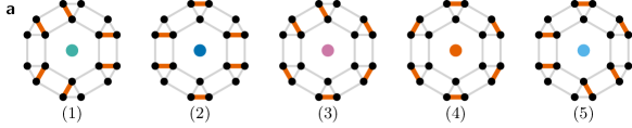
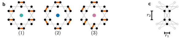
Figure S1: Depiction of the zero-field ground-state plaquette types in the $J_{1}$-$J_{2}$ (a) and $J_{1}$-$J_{3}$ (b) TFIM and of a unit cell on the lattice (c). In (a) and (b), ferromagnetic bonds are drawn in orange, antiferromagnetic bonds in light gray. Each of the depicted plaquette types is a representative of all plaquettes related by rotations. In (c), the black dots and light gray lines show the sites and bonds on the ruby lattice which are parts of its unit cell. The dashed lines and gray circles in the unit cell indicate its integration into the lattice but are not part of the unit cell itself.

For the $J_{1}$-$J_{2}$ TFIM with $J_{3}=0$ and $J_{1,2}>0$ we find five types of ground-state plaquettes as depicted in Fig. S1a. Note that the depiction in terms of ferromagnetic and antiferromagnetic bonds does not specify the orientation of the respective spins, giving rise to a global spin flip symmetry. We define each plaquette-type to include all plaquettes related to the one depicted by rotations. On the full lattice we find an extensive number of possibilities to combine those five types of plaquette configurations as illustrated in Fig. S2a, resulting in an extensively degenerate ground-state manifold. Note, an extensive ground-state degeneracy means that for large systems, the logarithm of the number of ground states scales with the system size.

For the $J_{1}$-$J_{3}$ TFIM with $J_{2}=0$ and $J_{1,3}>0$ we find three types of ground-state plaquettes as depicted in Fig. S1b. Again, each of those plaquette types yields multiple explicit spin configurations. Note, however, that none of the spin configurations which are a ground state for the $J_{1}$-$J_{3}$ case are a ground state for the $J_{1}$-$J_{2}$ case and vice versa, even though the configurations of ferromagnetic bonds look the same. On the full lattice we find an extensive number of possibilities to combine the three types of plaquette configurations as illustrated in Fig. S2b, resulting again in an extensively degenerate ground-state manifold.

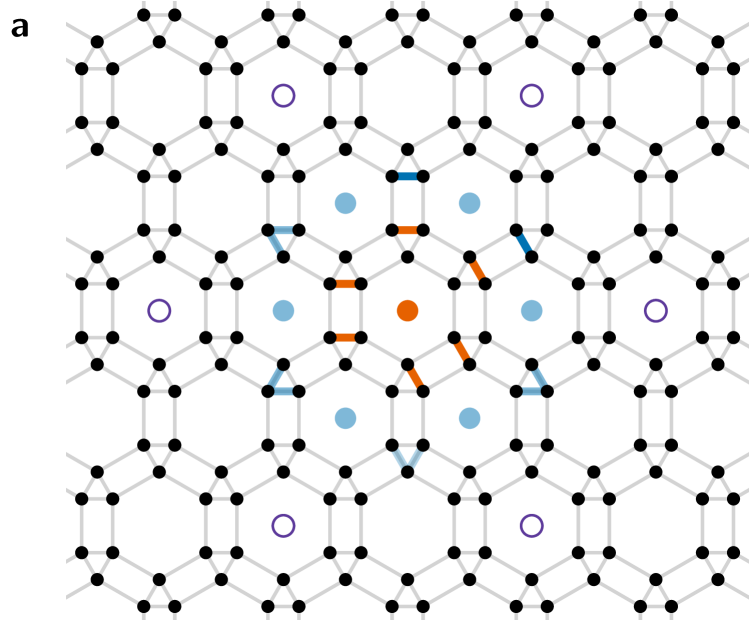
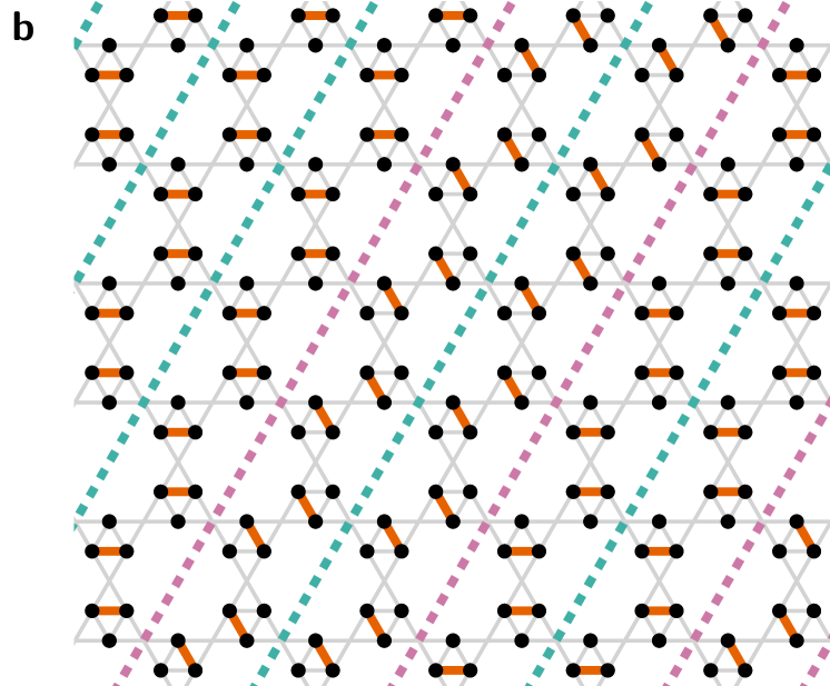
Figure S2: Illustration of the extensive ground-state degeneracy in the zero-field limit of the $J_{1}$-$J_{2}$ (a) and $J_{1}$-$J_{3}$ (b) case.
(a) Choosing the configuration of a central plaquette ( ), exemplarily type-(5) with ferromagnetic bonds in orange) places constraints on the six surrounding plaquettes ( ): dark blue lines resemble enforced ferromagnetic bonds, while light blue lines resemble the freedom of choosing one of the two respective bonds to be ferromagnetic. In the second-to-next surrounding circle, six plaquettes ( ) have no fixed ferromagnetic bonds and their configuration can be chosen from at least two plaquette types.
(b) The exemplary ground-state configuration (ferromagnetic bonds in orange) consists of stripes of different plaquette types (indicated by dashed lines). Next to a type-(1) stripe ( ) one can always place either another type-(1) stripe or a type-(3) stripe ( ) and vice versa.

For the full $J_{1}$-$J_{2}$-$J_{3}$ TFIM with $J_{1,2,3}>0$ and $J_{1}>J_{2,3}$, the lattice contains additional $J_{1}$-$J_{2}$-$J_{3}$-triangles (see Fig. S1c). Since all $J_{1}$-triangles have exactly one ferromagnetic $J_{1}$ bond, in 1/3 of those triangles the $J_{1}$ bond is ferromagnetic. For the remaining 2/3 of those triangle, this results in one additional ferromagnetic $J_{2}$- or $J_{3}$-bond per triangle. The energy per site is given by $\frac{1}{3}J_{1}+\chi\frac{2}{3}J_{2}+(1-\chi)\frac{2}{3}J_{3}$ with $\chi\in[0,1]$ depending on the ratio $J_{2}/J_{3}$. We distinguish the following three cases. If $J_{2}>J_{3}$, it is energetically beneficial for all $J_{2}$ bonds to be antiferromagnetic and we find $2/3$ ferromagnetic $J_{3}$ bonds. With $\chi=0$ the energy per site is $\frac{1}{3}J_{1}+\frac{2}{3}J_{3}$. Configurations with zero ferromagnetic $J_{2}$ bonds are exactly the $J_{1}$-$J_{2}$ ground states, which thus realize the ground states of the $J_{1}$-$J_{2}$-$J_{3}$ model with $J_{2}>J_{3}$. There exist no configurations with a smaller number of ferromagnetic bonds. The same holds for $J_{3}>J_{2}$ with $J_{2}$ and $J_{3}$ interchanged and $\chi=1$.

If $J_{2}=J_{3}$, additional frustration is present as the two bonds can not be distinguished and the energy per site is $\frac{1}{3}J_{1}+\frac{2}{3}J_{2}$ independent of $\chi$. In this case, all zero-field $J_{1}$-$J_{2}$ and $J_{1}$-$J_{3}$ ground states are ground states. Simultaneously, we find multiple further ground states: the ground-state plaquettes of the $J_{1}$-$J_{2}$ and $J_{1}$-$J_{3}$ model can be mixed and we also find further possible plaquette configurations. Thus, an enhanced ground-state degeneracy is present.

II.2 Leading order low-field effects

In the following we illustrate our analysis of the leading order processes in the limit of a small transverse magnetic field $h$ in the limiting cases of the $J_{1}$-$J_{2}$ and $J_{1}$-$J_{3}$ TFIM, for which we perform degenerate perturbation theory in the transverse field around $h=0$ using Takahashi’s method [1] (see Sec. I.1).

II.2.1 $J_{1}$-$J_{2}$ case

Diagonal corrections - We calculate diagonal corrections to the zero-field ground-state energy of the $J_{1}$-$J_{2}$ TFIM up to order four in the field $h$. For this we note that every zero-field plaquette in Fig. S1 and thus every zero-field ground state can be constructed from the three unit-cell configurations depicted in Fig. S3. As all processes relevant up to fourth order are contained within such a unit cell, the respective ground-state energy correction of any zero-field state can be calculated from the corrections of those three unit cells which we do in the following.

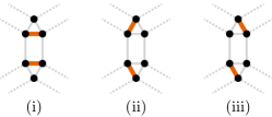
Figure S3: Unit-cell configurations appearing in zero-field ground states in the $J_{1}$-$J_{2}$ TFIM. Ferromagnetic bonds are drawn in orange, antiferromagnetic bonds in light gray. Antiferromagnetic $J_{2}$ bonds leaving the unit cell are drawn as dotted lines and have to be taken into account for the calculation of the corrections of the ground-state energy.

The unperturbed Hamiltonian is given by $\tilde{\mathcal{H}}_{0}$ in Eq. (S13) and yields the unperturbed ground-state energy

$$E_{0}^{(0)}=2J_{1}\,$$ (S14)

for all three unit cells. The perturbation $\mathcal{V}=\sum_{i}\sigma_{i}^{x}$ with perturbation parameter $\lambda=h\ll J$ only yields nonzero corrections for even orders in $h$. For the calculations it is illustrative to distinguish the sites in a zero-field unit cell by whether they are connected to one or zero ferromagnetic $J_{1}$ bonds and we introduce the notion of (anti)ferromagnetic sites, implying that the site has (zero) one ferromagnetic $J_{1}$ bond(s).

The second-order ground-state energy correction includes all processes acting twice on the same site. The contribution of a process depends only on whether the site is ferro- or antiferromagnetic, yielding the same contribution for all three unit cells:

$$E_{0}^{(2)}=-h^{2}\left(2\cdot\frac{1}{2J_{1}+2J_{2}}+4\cdot\frac{1}{2J_{2}}\right)\,.$$ (S15)

The fourth-order ground-state energy correction as given in Eq. (S3) contains summands consisting of two consecutive second-order processes, which are the same for all unit cells, and a purely fourth-order process acting on two interacting spins which distinguishes the unit cells energetically. The result of a process depends on whether the two involved sites are both ferromagnetic, both antiferromagnetic or one of each. For processes acting on two spins interacting via a $J_{1}$ bond, this implies that the result depends only on whether the bond itself is ferro- or antiferromagnetic, yielding the same contribution for all unit cells. The antiferromagnetic $J_{2}$ bonds however connect different types of sites for the three unit cells and respective fourth-order processes distinguish the unit cells energetically as follows:

$$E_{J_{2}}^{(4)}(\mathrm{i}) =-h^{4}\cdot 8\cdot\left(\frac{1}{2J_{2}}\right)^{3}\,,$$ (S16)

$$E_{J_{2}}^{(4)}(\mathrm{ii}) =-h^{4}\cdot\left(4\cdot\left(\frac{1}{2J_{2}}\right)^{3}+4\cdot\frac{1}{4J_{1}+2J_{2}}\cdot\left(\frac{1}{2J_{1}+2J_{2}}\right)^{2}\right)\,,$$ (S17)

$$E_{J_{2}}^{(4)}(\mathrm{iii}) =-h^{4}\cdot 2\cdot\frac{1}{2J_{1}+2J_{2}}\cdot\left(\frac{1}{2J_{2}}+\frac{1}{2J_{1}+2J_{2}}\right)^{2}\,.$$ (S18)

From this we find the following hierarchy of energy lowering corrections $E_{J_{2}}^{(4)}$ for arbitrary ${J_{1},J_{2}>0}$:

$$|E_{J_{2}}^{(4)}(\mathrm{i})|>|E_{J_{2}}^{(4)}(\mathrm{ii})|>|E_{J_{2}}^{(4)}(\mathrm{iii})|\,.$$ (S19)

As all other contributions to the fourth-order correction yield the same result for all three unit cells this defines the overall hierarchy of the unit cells up to fourth order, $(\mathrm{i})\to(\mathrm{ii})\to(\mathrm{iii})$. We confirm this analytically derived result by a numeric evaluation of the respective ground-state energy correction of the unit cells for $J_{1}=J_{2}$.

We continue by discussing the implications regarding the energy splitting of zero-field ground-states on the full lattice. All zero-field plaquettes in Fig. S1 contain the same fraction of 1/3 of the energetically most beneficial unit cell (i). For this statement, we also consider that a ferromagnetic bond along the outer hexagon of a plaquette enforces the continuation to a unit cell of type (i) in order to yield a valid zero-field ground state. The most beneficial plaquettes are thus the ones maximizing the number of unit cell (ii), i. e., plaquettes (1) and (4). The respective zero-field ground states containing only those plaquettes realize $\sqrt{3}\times\sqrt{3}$ clock-ordered structures on an underlying triangular lattice as depicted in the left panel in Fig. S4 and the zero-field ground-state degeneracy is lifted in a diagonal order-by-disorder scenario in fourth order in the magnetic field.

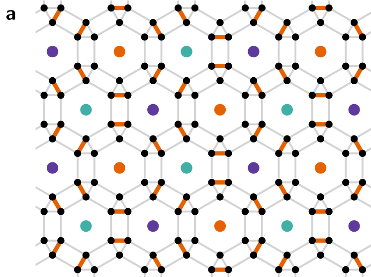
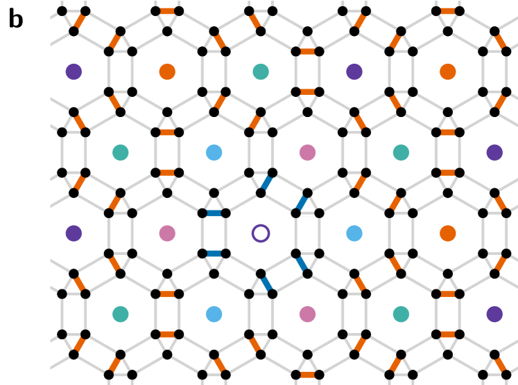
Figure S4: Two zero-field ground state configurations of the $J_{1}$-$J_{2}$ TFIM. The colored dots indicate the plaquette types with the following color code:   type (1),   and   type ($1^{\prime}$),   type (3),   type (4),   type (5).
(a) The zero-field ground-state configuration containing only type-(1) and type-(4) plaquettes. Here we explicitly distinguish the rotated type-(1) plaquettes as type-($1^{\prime}$) in order to illustrate the emergent $\sqrt{3}\times\sqrt{3}$ order. We find that states which exhibit such a clock order are selected from the zero-field ground-state manifold by a small transverse magnetic field in fourth order.
(b) The configuration resulting from the one in the left panel by a resonance of the type-(1) plaquette marked with   (ferromagnetic bonds in dark blue) to type ($1^{\prime}$) (compare Fig. S5), showing the presence of the resonating sixth-order process on the full lattice.

Off-diagonal corrections - On the level of single plaquettes we find the lowest-order off-diagonal process within the zero-field ground-state manifold to be a sixth-order process acting on the six sites of the inner hexagon a type-(1) plaquette. This is equivalent to a rotation of the plaquette by $60^{\circ}$ into a type-($1^{\prime}$) plaquette as shown in Fig. S5.

Figure S5: Illustration of the lowest-order off-diagonal process contributing to the effective low-field description of the $J_{1}$-$J_{2}$ TFIM. Applying a spin-flip to the six spins along the inner hexagon of a type-(1) plaquette, highlighted by gray shadows, switches the position of the ferromagnetic $J_{1}$ bond at each of those spins as shown. The resulting configuration is equivalent to the initial configuration rotated clockwise by $60^{\circ}$ and thus also a zero-field ground state we term type-($1^{\prime}$). Applying the same spin flip sequence for a second time results in the initial ground state.

We illustrate the presence of this process on the infinite lattice in Fig. S4. We find that mapping between plaquettes of type (1) and ($1^{\prime}$) within an arbitrary zero-field ground state changes each neighboring plaquette into another valid zero-field ground-state plaquette. Thus, the sixth-order process on type-(1) plaquettes induces resonances between different zero-field ground states. The respective ground states with maximal density of type-(1) and ($1^{\prime}$) plaquettes are the same $\sqrt{3}\times\sqrt{3}$ clock-ordered structures that are selected by diagonal energy corrections in order four in the magnetic field (see Fig. S4a).

Summarizing, fourth-order diagonal energy corrections lift the zero-field ground-state degeneracy and benefit the subspace of $\sqrt{3}\times\sqrt{3}$ clock-ordered states with maximal density of type-(1) and ($1^{\prime}$) plaquettes. The leading-order off-diagonal process in sixth order induces resonances between those type-(1) and ($1^{\prime}$) plaquettes which are thus maximized within the subspace selected by the fourth-order diagonal corrections. We write down an effective low-field description as a sum over all plaquettes on the lattice,

$$\mathcal{H}_{\mathrm{eff}}=\bar{E}_{0} +\frac{h^{4}}{2}\sum_{\hskip 1.42271pt\includegraphics[height=9.0pt,valign={c}]{symbol7.pdf}\hskip 1.42271pt}\bigg{(}\big{(}\underbrace{3E_{J_{2}}^{(4)}(\mathrm{i})+3E_{J_{2}}^{(4)}(\mathrm{ii})}_{=:E_{J_{2}}^{(4)}(\leavevmode\hbox{$\vbox{\hbox{\resizebox{}{}{{\leavevmode\hbox{\set@color{ \leavevmode\hbox to5.69pt{\vbox to5.69pt{\text{[drawing]}}}}}}}}}$})}\big{)}\ket{\hskip 1.42271pt\includegraphics[height=20.0pt,valign={c}]{symbol1.pdf}\hskip 1.42271pt}\bra{\hskip 1.42271pt\includegraphics[height=20.0pt,valign={c}]{symbol1.pdf}\hskip 1.42271pt}+\big{(}\underbrace{2E_{J_{2}}^{(4)}(\mathrm{i})+4E_{J_{2}}^{(4)}(\mathrm{iii})}_{=:E_{J_{2}}^{(4)}(\leavevmode\hbox to5.69pt{\vbox to5.69pt{\text{[drawing]}}})}\big{)}\ket{\hskip 1.42271pt\includegraphics[height=20.0pt,valign={c}]{symbol3.pdf}\hskip 1.42271pt}\bra{\hskip 1.42271pt\includegraphics[height=20.0pt,valign={c}]{symbol3.pdf}\hskip 1.42271pt}$$ (S20)

$$+\big{(}\underbrace{1E_{J_{2}}^{(4)}(\mathrm{i})+3E_{J_{2}}^{(4)}(\mathrm{ii})+2E_{J_{2}}^{(4)}(\mathrm{iii})}_{=:E_{J_{2}}^{(4)}(\leavevmode\hbox to5.69pt{\vbox to5.69pt{\text{[drawing]}}})}\big{)}\ket{\hskip 1.42271pt\includegraphics[height=20.0pt,valign={c}]{symbol4.pdf}\hskip 1.42271pt}\bra{\hskip 1.42271pt\includegraphics[height=20.0pt,valign={c}]{symbol4.pdf}\hskip 1.42271pt}+\underbrace{6E_{J_{2}}^{(4)}(\mathrm{ii})}_{=:E_{J_{2}}^{(4)}(\leavevmode\hbox to5.69pt{\vbox to5.69pt{\text{[drawing]}}})}\ket{\hskip 1.42271pt\includegraphics[height=20.0pt,valign={c}]{symbol5.pdf}\hskip 1.42271pt}\bra{\hskip 1.42271pt\includegraphics[height=20.0pt,valign={c}]{symbol5.pdf}\hskip 1.42271pt}+$$

$$+\big{(}\underbrace{2E_{J_{2}}^{(4)}(\mathrm{i})+2E_{J_{2}}^{(4)}(\mathrm{ii})+2E_{J_{2}}^{(4)}(\mathrm{iii})}_{=:E_{J_{2}}^{(4)}(\leavevmode\hbox to5.69pt{\vbox to5.69pt{\text{[drawing]}}})}\big{)}\ket{\hskip 1.42271pt\includegraphics[height=20.0pt,valign={c}]{symbol6.pdf}\hskip 1.42271pt}\bra{\hskip 1.42271pt\includegraphics[height=20.0pt,valign={c}]{symbol6.pdf}\hskip 1.42271pt}\bigg{)}+h^{6}\sum_{\hskip 1.42271pt\includegraphics[height=9.0pt,valign={c}]{symbol7.pdf}\hskip 1.42271pt}\frac{63}{16J_{2}^{5}}\left(\ket{\hskip 1.42271pt\includegraphics[height=20.0pt,valign={c}]{symbol1.pdf}\hskip 1.42271pt}\bra{\hskip 1.42271pt\includegraphics[height=20.0pt,valign={c}]{symbol2.pdf}\hskip 1.42271pt}+\mathrm{h.c.}\right)$$

$$=:\bar{E}_{0} +\frac{h^{4}}{2}\sum_{\hskip 1.42271pt\includegraphics[height=8.0pt,valign={c}]{symbol7.pdf}\hskip 1.42271pt}\quad\sum_{\mathclap{\begin{subarray}{c}\leavevmode\hbox to5.69pt{\vbox to5.69pt{\text{[drawing]}}}=\leavevmode\hbox{$\vbox{\hbox{\resizebox{}{}{{\leavevmode\hbox{\set@color{ \leavevmode\hbox to5.69pt{\vbox to5.69pt{\text{[drawing]}}}}}}}}}$},\leavevmode\hbox to5.69pt{\vbox to5.69pt{\text{[drawing]}}},\leavevmode\hbox to5.69pt{\vbox to5.69pt{\text{[drawing]}}},\\ \quad\leavevmode\hbox to5.69pt{\vbox to5.69pt{\text{[drawing]}}},\leavevmode\hbox to5.69pt{\vbox to5.69pt{\text{[drawing]}}}\end{subarray}}}\quad\left(E_{J_{2}}^{(4)}({\leavevmode\hbox{$\vbox{\hbox{\resizebox{}{}{{\leavevmode\hbox{\set@color{ \leavevmode\hbox to5.69pt{\vbox to5.69pt{\text{[drawing]}}}}}}}}}$}})\ket{\hskip 1.42271pt\includegraphics[height=20.0pt,valign={c}]{symbol8.pdf}\hskip 1.42271pt}\bra{\hskip 1.42271pt\includegraphics[height=20.0pt,valign={c}]{symbol8.pdf}\hskip 1.42271pt}\right)+h^{6}\sum_{\hskip 1.42271pt\includegraphics[height=8.0pt,valign={c}]{symbol7.pdf}\hskip 1.42271pt}E_{\mathrm{res}}^{(6)}\left(\ket{\hskip 1.42271pt\includegraphics[height=20.0pt,valign={c}]{symbol1.pdf}\hskip 1.42271pt}\bra{\hskip 1.42271pt\includegraphics[height=20.0pt,valign={c}]{symbol2.pdf}\hskip 1.42271pt}+\mathrm{h.c.}\right)$$

with constant $\bar{E}_{0}$ containing perturbative contributions which are equal for all ground states. In the diagonal part each of the five plaquette types is defined to include plaquettes related to the depicted one by symmetry operations like rotations like before. In the off-diagonal part we explicitly write down the plaquette types (1) and ($1^{\prime}$) related by rotation as it is physically relevant for the resonance. Each relevant diagonal fourth-order process acting on the $J_{2}$ bonds is part of two plaquettes and thus considered twice in the sum over plaquettes which is accounted for by a factor 1/2.

We note that the resonance of a type-(1) plaquette within a clock-ordered state as illustrated in Fig. S4 leaves the subspace of zero-field ground states benefited by diagonal corrections in fourth order, as six unit cells (ii) are turned into unit cell (iii). The subspaces of one resonated plaquette and zero resonated plaquettes have an energy splitting of ${6|E_{J_{2}}^{(4)}(\mathrm{ii})-E_{J_{2}}^{(4)}(\mathrm{iii})|}$. This can be extended to multiple resonated plaquettes. Note that resonating a second plaquette does not necessarily turn six unit cells from (ii) to (iii): if the two resonated plaquettes are connected by a unit cell, this unit cell undergoes the process $(\mathrm{ii})\to(\mathrm{iii})\to(\mathrm{ii})$ upon the two resonating processes, i. e., it is of type (ii) in the end and hence only 11 unit cells are turned from (ii) to (iii).

II.2.2 $J_{1}$-$J_{3}$ case

Diagonal corrections - We calculate diagonal corrections to the zero-field ground-state energy of the $J_{1}$-$J_{3}$ TFIM up to order four in $h$ analogous to the procedure for the $J_{1}$-$J_{2}$ TFIM described in Sec. II.2.1. As each zero-field ground-state configuration is built from different mixtures of the three unit-cell configurations illustrated in Fig. S6, we determine the most beneficial ground state by ranking those three unit cells by their energy corrections.

Figure S6: Unit-cell configurations appearing in zero-field ground states in the $J_{1}$-$J_{3}$ TFIM. Ferromagnetic bonds are drawn in orange, antiferromagnetic bonds in light gray. Antiferromagnetic $J_{3}$ bonds leaving the unit cell are drawn as dotted lines and have to be taken into account for the calculation of the right corrections of the ground-state energy.

We note that the three configurations of ferromagnetic $J_{1}$ bonds look like the ones in the unit cells for the $J_{1}$-$J_{2}$ case (compare Fig. S3) and the unperturbed ground-state energy of the three unit cells is equally given by $E_{0}^{(0)}=2J_{1}$. However, the $J_{2}$ and $J_{3}$ bonds connect different sites within the unit cells such that the spin configurations may differ. We find that unit cells (i) from the two models are equivalent regarding the explicit spin configuration and geometry of (anti)ferromagnetic bonds. Further, unit cell (ii) in the $J_{1}$-$J_{3}$ case is equivalent to unit cell (iii) in the $J_{1}$-$J_{2}$ case and vice versa. Consequently, we find that the energy corrections and the resulting energetic hierarchy of unit cells are equivalent to the $J_{1}$-$J_{2}$ case for $J_{2}\to J_{3}$ and upon swapping (ii) and (iii). In second order, the correction to the ground-state energy is given by

$$E_{0}^{(2)}=-h^{2}\left(4\cdot\frac{1}{2J_{3}}+2\cdot\frac{1}{2J_{1}+2J_{3}}\right)\,.$$ (S21)

for all three unit cells. In fourth order, the three unit cells are distinguished by purely fourth-order processes acting on two spins connected by a $J_{3}$ bond,

$$E_{J_{3}}^{(4)}(\mathrm{i}) =-h^{4}\cdot 8\cdot\left(\frac{1}{2J_{3}}\right)^{3}\,,$$ (S22)

$$E_{J_{3}}^{(4)}(\mathrm{ii}) =-h^{4}\cdot 2\cdot\frac{1}{2J_{1}+2J_{3}}\cdot\left(\frac{1}{2J_{3}}+\frac{1}{2J_{1}+2J_{3}}\right)^{2}\,$$ (S23)

$$E_{J_{3}}^{(4)}(\mathrm{iii}) =-h^{4}\cdot\left(4\cdot\left(\frac{1}{2J_{3}}\right)^{3}+4\cdot\frac{1}{4J_{1}+2J_{3}}\cdot\left(\frac{1}{2J_{1}+2J_{3}}\right)^{2}\right)\,,$$ (S24)

resulting in the overall energetic hierarchy of the unit cells up to fourth order, $(\mathrm{i})\to(\mathrm{iii})\to(\mathrm{ii})$, for arbitrary $J_{1},J_{3}>0$.

Similar to the $J_{1}$-$J_{2}$ case, all $J_{1}$-$J_{3}$ zero-field plaquettes in Fig. S1 enforce the same fraction of 1/3 of the energetically most beneficial unit cell (i). Plaquettes of type-(1) maximize the number of the second-most-beneficial unit cell (iii). The configuration on the full lattice which maximizes the number of such type-(1) plaquettes is the one containing only type-(1) plaquettes exhibiting $\bm{k}=(0,0)$ order, as illustrated in Fig. S7, and the ground-state degeneracy at zero magnetic field is lifted in a diagonal order-by-disorder scenario in fourth order in the magnetic field.

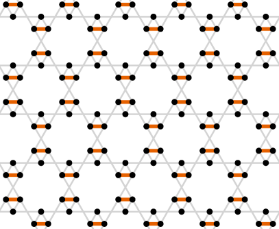
Figure S7: Zero-field ground-state of the $J_{1}$-$J_{3}$ TFIM containing only type-(1) plaquettes which is favored by the a small transverse magnetic field in fourth order. Orange lines resemble ferromagnetic bonds, light gray lines antiferromagnetic ones.

Off-diagonal corrections - In contrast to the $J_{1}$-$J_{2}$ TFIM we find no resonating process between different zero-field ground states in any finite order in $h$, as can be understood from the geometry of $J_{3}$ bonds which form decoupled chains over the full lattice (compare straight gray lines in Fig. S7) with each site being contained in exactly one chain. In a zero-field ground state, all $J_{3}$ bonds are antiferromagnetic and the spins are aligned antiparallel along all chains. Mapping between different zero-field ground states requires inverting an entire chain of spins and thus an infinite order in $h$.

In summary, we express the effective low-field model in the $J_{1}$-$J_{3}$ model as a sum over all unit cells on the lattice,

$$\mathcal{H}_{\mathrm{eff}} =\bar{E}_{0}+h^{4}\sum_{\hskip 1.42271pt\includegraphics[angle={90},height=5.0pt,valign={c}]{symbol12.pdf}\hskip 1.42271pt}\left(E_{J_{3}}^{(4)}(\mathrm{i})\ket{\hskip 1.42271pt\includegraphics[angle={90},height=8.0pt,valign={c}]{symbol9.pdf}\hskip 1.42271pt}\bra{\hskip 1.42271pt\includegraphics[angle={90},height=8.0pt,valign={c}]{symbol9.pdf}\hskip 1.42271pt}+E_{J_{3}}^{(4)}(\mathrm{ii})\ket{\hskip 1.42271pt\includegraphics[angle={90},height=8.0pt,valign={c}]{symbol10.pdf}\hskip 1.42271pt}\bra{\hskip 1.42271pt\includegraphics[angle={90},height=8.0pt,valign={c}]{symbol10.pdf}\hskip 1.42271pt}+E_{J_{3}}^{(4)}(\mathrm{iii})\ket{\hskip 1.42271pt\includegraphics[angle={90},height=8.0pt,valign={c}]{symbol11.pdf}\hskip 1.42271pt}\bra{\hskip 1.42271pt\includegraphics[angle={90},height=8.0pt,valign={c}]{symbol11.pdf}\hskip 1.42271pt}\right)\,,$$ (S25)

with constant $\bar{E}_{0}$ containing perturbative contributions which are equal for all ground states.

III High-field series expansions

In this section we discuss our results in the limit of high magnetic fields, $h\gg J$, of the $J_{1}$-$J_{2}$-$J_{3}$ TFIM. Applying the pCUT method in combination with a graph decomposition (see Sec. I) we obtain the one quasi-particle effective Hamiltonian $\mathcal{H}_{\mathrm{eff}}$ in order 9 in $\lambda=J/2h$ for the general $J_{1}$-$J_{2}$-$J_{3}$ TFIM, in order 10 for the reduced $J_{1}$-$J_{2}$ and $J_{1}$-$J_{3}$ TFIM, and in order 11 for the respective limiting cases $J_{1}=J_{2}$ and $J_{1}=J_{3}$. Note that we define the three interaction strengths $J_{1,2,3}$ to be related to each other, with the explicit definitions stated in the respective sections, and thus only consider a single perturbation parameter $\lambda$.

III.1 Dispersion

As the ruby lattice has a unit cell containing six sites the one quasi-particle effective Hamiltonian reduces to a $6\times 6$ matrix $h_{lm}(\bm{k})$ with $l,m\in{1,2,\ldots,6}$ in momentum space using a Fourier transformation. Due to the lattice symmetries, this matrix exhibits the following relations:

$$h_{11}(k_{1},k_{2})=h_{66}(k_{1},k_{2})=h_{22}(k_{1},k_{1}-k_{2}) =h_{55}(k_{1},k_{1}-k_{2})=h_{33}(k_{1}-k_{2},k_{1})=h_{44}(k_{1}-k_{2},k_{1})$$ (S26)

$$h_{12}(k_{1},k_{2})=h_{56}(k_{1},k_{2}) =h_{13}(k_{2},k_{1})=h_{46}(k_{2},k_{1})$$

$$h_{14}(k_{1},k_{2})=h_{36}(k_{1},k_{2}) =h_{15}(k_{2},k_{1})=h_{26}(k_{2},k_{1})$$

$$h_{23}(k_{1},k_{2}) =h_{45}(k_{1},k_{2})$$

$$h_{24}(k_{1},k_{2}) =h_{35}(k_{1},k_{2})$$

$$h_{25}(k_{1},k_{2}) =h_{34}(k_{2},k_{1})$$

$$h_{\alpha\beta} =(h_{\beta\alpha})^{*}$$

and only the seven elements $h_{11},h_{12},h_{14},h_{16},h_{23},h_{24},h_{25}$ have to be calculated. We obtain the dispersion containing six energy bands by diagonalizing $h(\bm{k})$, where we find a qualitative difference between the $J_{1}$-$J_{2}$ and the $J_{1}$-$J_{3}$ TFIM which extends to the full $J_{1}$-$J_{2}$-$J_{3}$ TFIM.

For the $J_{1}$-$J_{2}$ case the six dispersive energy bands qualitatively take the shape depicted in Fig. S8 exemplarily for the case $J_{1}=J_{2}$ with $J_{1}/2h=0.2$. We locate the minima of the dispersion, corresponding to the one quasi-particle excitation gap $\Delta$, at ${\bm{k}=(2\pi/3,-2\pi/3)}$ for all finite ratios $J_{1}/J_{2}>0$.

For the $J_{1}$-$J_{3}$ case the six dispersive energy bands qualitatively take the shape depicted in Fig. S9 exemplarily for the case $J_{1}=J_{3}$ with $J_{1}/2h=0.2$. We locate the minima of the dispersion at $\bm{k}=(0,0)$ for all finite ratios $J_{1}/J_{3}>0$.

For the full $J_{1}$-$J_{2}$-$J_{3}$ case we find that the dispersion qualitatively depends on the ratio $J_{2}/J_{3}$. For $J_{2}>J_{3}$ we find the same qualitative dispersion as for the pure $J_{1}$-$J_{2}$ TFIM, while for $J_{3}>J_{2}$ the dispersion resembles the one of the pure $J_{1}$-$J_{3}$ TFIM.

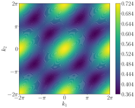
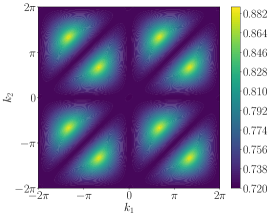
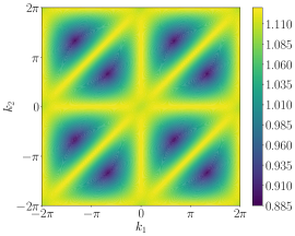
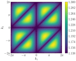
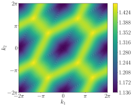
Figure S8: One quasi-particle dispersion in the $J_{1}$-$J_{2}$ TFIM for $J_{1,2}/2h=0.2$ in units of $2h$. The momenta $k_{1},k_{2}$ are defined with respect to the lattice vectors $\bm{t}_{1},\bm{t}_{2}$.

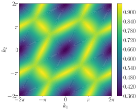
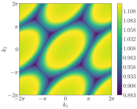
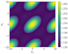
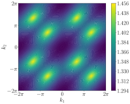
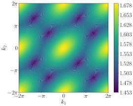
Figure S9: One quasi-particle dispersion in the $J_{1}$-$J_{3}$ TFIM for $J_{1,3}/2h=0.2$ in units of $2h$. The momenta $k_{1},k_{2}$ are defined with respect to the lattice vectors $\bm{t}_{1},\bm{t}_{2}$.

III.2 Elementary excitation gap

The elementary excitation gap $\Delta(\lambda)$ is given by the one quasi-particle energy at the minimum of the dispersion and obtained as a series in $\lambda$ by explicit diagonalization of the effective Hamiltonian at the respective gap momentum. We perform DlogPadé extrapolations (compare Sec. I.4) on $\Delta(\lambda)$ to approximate the assumed underlying power-law behavior $\Delta\propto|\lambda-\lambda_{c}|^{z\nu}$ of the elementary excitation gap and extract the critical point $\lambda_{c}$ and the critical exponent $z\nu$.

III.2.1 $J_{1}$-$J_{2}$ and $J_{1}$-$J_{3}$ case

We first consider the cases $J_{1}=J_{2}$ and $J_{1}=J_{3}$ in the reduced $J_{1}$-$J_{2}$ and $J_{1}$-$J_{3}$ models in detail. The bare series of the excitation gap $\Delta(\lambda)$ in order $r=11$ in $\lambda=J_{1}/2h$ are shown in Fig. S10 (first row) alongside extrapolants obtained from orders $r\geq 9$ and with $|L-M|\leq 3$. For both cases we find a critical point $\lambda_{c}$ where the gap closes and extract the critical exponent $z\nu$. We structure the extrapolants $dP[L,M]$ into families with the same $d=L-M$ and plot the critical point and exponent as a function of the order $r=L+M+1$ in Fig. S10, taking only extrapolants with $|L-M|\leq 3$ into account. To obtain an estimate for $\lambda_{c}$ and $z\nu$ we average over the extrapolants of the highest order of all considered families. We obtain $\lambda_{c}=0.289\pm 0.004$ and $z\nu=0.806\pm 0.056$ for the $J_{1}=J_{2}$ case and $\lambda_{c}=0.272\pm 0.006$ and $z\nu=0.632\pm 0.101$ for the $J_{1}=J_{3}$ case.

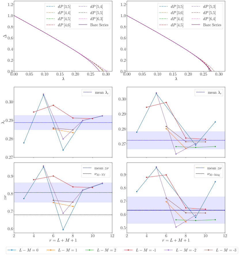
Figure S10: Results from high-field series expansions in the $J_{1}$-$J_{2}$ TFIM with $J_{1}=J_{2}$ (left panels) and the $J_{1}$-$J_{3}$ TFIM with $J_{1}=J_{3}$ (right panels).
First row: Elementary excitation gap $\Delta(\lambda)$ in units of $2h$ as a function of $\lambda=J_{1}/2h$. The plots show the bare series in order $r=11$ alongside DlogPadé extrapolants obtained from orders $r\geq 9$ within families $|L-M|\leq 3$.
Second and third row: Convergence behavior of the critical points $\lambda_{c}$ (second row) and critical exponents $z\nu$ (third row) extracted from the DlogPadé extrapolants $dP[L,M]$ in the considered order $r=L+M+1$. The extrapolants are structured into families by connecting extrapolants with the same $d=L-M$. We show only extrapolants with $|L-M|\leq 3$. To obtain a mean value for $\lambda_{c}$ and $z\nu$ we average over the extrapolants of highest order for each shown family. The calculated means $\lambda_{c}=0.289\pm 0.004$ and $z\nu=0.806\pm 0.056$ for $J_{1}=J_{2}$ and $\lambda_{c}=0.272\pm 0.006$ and $z\nu=0.632\pm 0.101$ for $J_{1}=J_{3}$ are drawn as a dashed blue lines, with the highlighted areas indicating the standard deviations of the individual extrapolants. The black dashed lines represent the literature values for $\nu_{\mathrm{3d-XY}}=0.67169(7)$ [10, 11] and $\nu_{\mathrm{3d-Ising}}=0.629971(4)$ [12] respectively.

We continue by discussing the $J_{1}$-$J_{2}$ and $J_{1}$-$J_{3}$ TFIM for arbitrary ratios $J_{1}/J_{2}$ and $J_{1}/J_{3}$ respectively, where we calculate the dispersion up to order $r=10$ in $\lambda=J/2h$. We define the two nonzero interaction strengths as

$$J_{1} =\cos(\theta)\,J\,,$$ (S27)

$$J_{2,3} =\sin(\theta)\,J\,.$$ (S28)

As noted in Sec. III.1, the gap momentum is independent from the ratio $J_{1}/J_{2,3}$ within the respective reduced model. In Fig. S11 we show the critical points $\lambda_{c}$ and the critical exponents $z\nu$ determined from selected (non-defective) DlogPadé extrapolants as a function of $\theta$ for both models. Note that the previously discussed cases $J_{1}=J_{2}$ and $J_{1}=J_{3}$ are recovered for $\theta=\pi/4$, respectively. However, $\theta=\pi/4$ corresponds to $J_{1}=J_{2,3}=J/\sqrt{2}$ in this parametrization which results in a rescaling of $\lambda_{c}$.

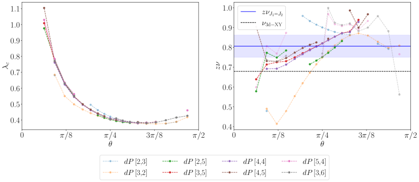
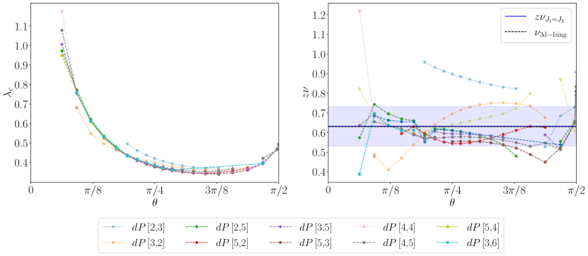
Figure S11: Critical points $\lambda_{c}$ (left panels) and critical exponents $z\nu$ (right panels) for various ratios of $J_{2}/J_{1}$ (upper panels) and $J_{3}/J_{1}$ (lower panels) parameterized by $\theta$ as given in the main text. The plots show the results obtained from individual selected DlogPadé extrapolants in different orders. Extrapolants which show deviations from the (qualitative) behavior of the bulk are shown in lighter opacities. The blue lines and shaded regions show the values $z\nu_{J_{1}=J_{2,3}}$ with their standard deviations as calculated in Sec. III.2.1, respectively. The black dashed lines in the right panels show the literature value for the assumed 3d-XY and 3d-Ising criticalities of the phase transition, $\nu_{\mathrm{3d-XY}}=0.67169(7)$ [10, 11] and $\nu_{\mathrm{3d-Ising}}=0.629971(4)$ [12].

The selected extrapolants show the same qualitative behavior regarding the extracted critical points $\lambda_{c}$ and we find a closing of the excitation gap for $\theta\in(0.1,1.47)$ in the $J_{1}$-$J_{2}$ TFIM, which corresponds to $J_{1}/J_{2}=\cot\theta\in(0.1,10)$, and for $\theta\in(0.1,1.57)$ in the $J_{1}$-$J_{3}$ TFIM, which corresponds to ${J_{1}/J_{2}\in(0.1,100)}$. Coming from the symmetric case $\theta=\pi/4$ and decreasing $\theta$, the critical point gets pushed to larger $\lambda$ as the limit of decoupled $J_{1}$-triangles is approached in both cases. For $\theta=\pi/2$ in the $J_{1}$-$J_{2}$ TFIM, the system consists of isolated hexagons and there is no phase transition, while in the $J_{1}$-$J_{3}$ TFIM, the system consists of decoupled $J_{3}$-chains with the critical point $\lambda_{c}=0.5$ from the one-dimensional TFIM. Regarding the critical exponents we find some more variety in the qualitative behavior. Nevertheless we can identify a consistent tendency among extrapolants of high orders. Within the $J_{1}$-$J_{2}$ TFIM, the critical exponent increases with $\theta$ while within the $J_{1}$-$J_{3}$ TFIM, the critical exponent decreases slightly with $\theta$. In both cases we argue that the critical exponent remains roughly constant, considering the range of deviation indicated by the results we obtain for $\theta=\pi/4$ respectively, as indicated by the blue shaded regions in Fig. S11.

III.2.2 Experimental realization of the $J_{1}$-$J_{2}$-$J_{3}$ TFIM

In the following we highlight two experimentally relevant cases of the $J_{1}$-$J_{2}$-$J_{3}$ TFIM which can be implemented on a Rydberg atom quantum simulator with appropriately fixed laser detuning. Interactions between excited Rydberg atoms are of van-der-Waals type and decay algebraically with the distance $r$ between atoms like $\sim r^{-6}$, which defines the relations between the $J_{i}$. The distances $r_{i}$ between the three nearest neighbors we consider in the series expansion depend on the aspect ratio $\rho$ of the ruby lattice as follows: setting $r_{1}=1$, $r_{2}=\rho$ and $r_{3}=(1+\rho^{2})^{1/2}$. Note that which site is the fourth-nearest neighbor depends on $\rho$, for $\rho>5/4$ we find $r_{4}=(\rho(\rho+\sqrt{3})+1)^{1/2}$ while for $\rho<5/4$ we find $r_{4}=\sqrt{3}\rho$. For all $\rho\geq 1$ we have $J_{i}\geq J_{i+1}$ for $i\in\mathbb{N}$.

The first case we highlight is the structure with the sites located on the links of a Kagome lattice, realized by the ruby lattice for an aspect ratio of $\rho=\sqrt{3}$. Here the interaction strengths as defined by the algebraic decay, $J_{i}=J_{1}r_{i}^{-6}$, are given by $J_{2}=J_{1}/27$ and $J_{3}=J_{1}/64$, neglecting all $J_{i}\leq J_{4}=J_{1}/364$. We depict our results for the excitation gap obtained by pCUT high-order high-field series expansions in $\lambda=J_{1}/2h$ and subsequent DlogPadé extrapolations in Fig. S12 (upper left panel) in analogous fashion to Fig. S10. The gap momentum is $\bm{k}=(2\pi/3,-2\pi/3)$ as $J_{1}>J_{2}>J_{3}$. The system is dominated by the $J_{1}$ interaction which defines isolated triangles with no phase transition. Considering only $J_{2}$ results in the energy gap as depicted in orange, which is very close to the results obtained from considering all three interaction. explaining why no phase transition can be detected within our perturbative approach.

The second case is the one of $\rho=1$, which results in $J_{1}=J_{2}$ and $J_{3}=J_{1}/8$, again neglecting all $J_{i}\leq J_{4}=J_{1}/27$. Our high-field results for the excitation gap are depicted in Fig. S12 (upper right panel). We find a gap momentum $\bm{k}=(2\pi/3,-2\pi/3)$ in line with previous results for $J_{1}>J_{2}>J_{3}$ with a quantum phase transition at $\lambda_{c}=0.301\pm 0.003$ ($C_{6}/\Omega=1.202\pm 0.012$) with exponent $z\nu=0.801\pm 0.046$ (values obtained by averaging over extrapolants of highest order for all families depicted in Fig. S12, lower panels).

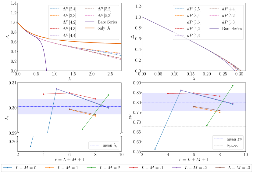
Figure S12: High-field results for two experimentally relevant cases. Upper panels: One quasi-particle excitation gap $\Delta$ in the $J_{1}$-$J_{2}$-$J_{3}$ TFIM with $\rho=\sqrt{3}$ (left) and $\rho=1$ (right) in units of $2h$ as a function of $\lambda=J_{1}/2h$. The bare series in the maximal order $r=9$ is shown along lower orders in lower opacities and the obtained DlogPadé extrapolants $dP[L,M]$ in orders $r\geq 7$ with in families $|L-M|\leq 3$ as a function of $\lambda=J_{1}/2h$. The thick orange line in the left panel shows the gap in the limit of $J_{2}=J_{3}=0$, where the lattice is decomposed into isolated triangles. Lower panels: Convergence behavior of the critical point $\lambda_{c}$ (left) and critical exponent $z\nu$ (right) for $\rho=1$ in the $J_{1}$-$J_{2}$-$J_{3}$ TFIM extracted from the DlogPadé extrapolants $dP[L,M]$ in the considered order $r=L+M+1$. The extrapolants are structured into families by connecting extrapolants with the same $d=L-M$. We show only extrapolants with $|L-M|\leq 3$. To obtain a mean value for $\lambda_{c}$ and $z\nu$ we average over the extrapolants of highest order for each shown family. The calculated means $\lambda_{c}=0.301\pm 0.003$ and $z\nu=0.801\pm 0.046$ for are drawn as a dashed blue lines, with the highlighted areas indicating the standard deviations of the individual extrapolants. The black dashed line represents the literature value for $\nu_{\mathrm{3d-XY}}=0.67169(7)$ [10, 11].