On the Energy Consumption of UAV Edge Computing in Non-Terrestrial Networks

Abstract

During the last few years, Unmanned Aerial Vehicles (UAVs) equipped with sensors and cameras have emerged as a cutting-edge technology to provide services such as surveillance, infrastructure inspections, and target acquisition. However, this approach requires UAVs to process data onboard, mainly for person/object detection and recognition, which may pose significant energy constraints as UAVs are battery-powered. A possible solution can be the support of Non-Terrestrial Networks (NTNs) for edge computing. In particular, UAVs can partially offload data (e.g., video acquisitions from onboard sensors) to more powerful upstream High Altitude Platforms (HAPs) or satellites acting as edge computing servers to increase the battery autonomy compared to local processing, even though at the expense of some data transmission delays. Accordingly, in this study we model the energy consumption of UAVs, HAPs, and satellites considering the energy for data processing, offloading, and hovering. Then, we investigate whether data offloading can improve the system performance. Simulations demonstrate that edge computing can improve both UAV autonomy and end-to-end delay compared to onboard processing in many configurations.

I Introduction

In the context of 6th generation (6G) wireless networks [1], Non-Terrestrial Network (NTN) is an emerging paradigm that consists of deploying aerial/space nodes such as Unmanned Aerial Vehicles (UAVs), High Altitude Platforms (HAPs) and satellites to improve the coverage and capacity of ground users when terrestrial infrastructure is not deployed, unavailable, or overloaded [2]. In particular, given their low cost and their versatility, UAVs can support applications such as surveillance, traffic control, disaster management, environmental monitoring, and high-precision agriculture [3, 4]. To enable these services, UAVs need to store and process data generated from local sensors (e.g., video acquisitions from video cameras), mainly to detect and recognize critical objects and/or potential dangers on the ground [5, 6]. However, data processing often involves running computationally demanding deep learning and computer vision algorithms onboard the UAV [5], which may not be compatible with the limited computational capacity and battery lifetime of these platforms. In fact, UAVs consume significant energy for hovering and propulsion, and data processing will further reduce their autonomy.

To solve this issue, UAVs can delegate the burden of data processing to more powerful computing servers located at the edge of the network, a paradigm referred to as (mobile) edge computing [7]. In this way, rotary-wing UAVs consume less power, and the processing can be performed even if the UAV has no processing units [8]. In these regards, the best choice would be to deploy the edge servers as close to the end users as possible to reduce the delays for data offloading and for the processed output to be returned. Edge servers can also be located on NTN nodes, for example on HAPs or Low Earth Orbit (LEO) satellites [9], so as to provide large and continuous geographical coverage even in rural/remote areas [10] or in the absence of pre-existing terrestrial infrastructures [11]. In our previous works, we studied the potential of NTN-assisted edge computing applied to vehicular [12] and Internet of Things (IoT) [13] networks. Specifically, we optimized the offloading rate to maximize the probability of real-time service given delay and computational capacity constraints. The integration of LEO satellites with UAVs has also been studied in [14], where the authors optimized the offloading rate to enable faster data processing. However, most of the literature tends to consider data generated on the ground and relayed to (or processed by) the UAV, and measure the performance of edge computing only in terms of delay, with limited considerations related to energy consumption.

To fill these gaps, in this paper we analyze a scenario where a swarm of UAVs collects sensory data that needs to be processed by an object detection algorithm. The processing can be performed locally onboard the UAVs, or data can be offloaded to an NTN edge computing server (either a HAP or a LEO satellite). Then, we develop an energy model to characterize the energy consumption of UAVs, HAPs, and LEO satellites for data processing and offloading, as well as for hovering and/or movement. Finally, we model the system as a set of D/M/1 queues, and investigate the impact of data offloading on the UAV battery autonomy and the end-to-end delay. We demonstrate that both HAP- and LEO-assisted edge computing can improve the autonomy and delay compared to onboard processing in many configurations.

The rest of the paper is organized as follows. In Sec. II we formulate our research problem and present our channel and delay models. In Sec. III we describe our energy model. In Sec. IV we provide numerical results. In Sec. V we conclude the paper with suggestions for future work.

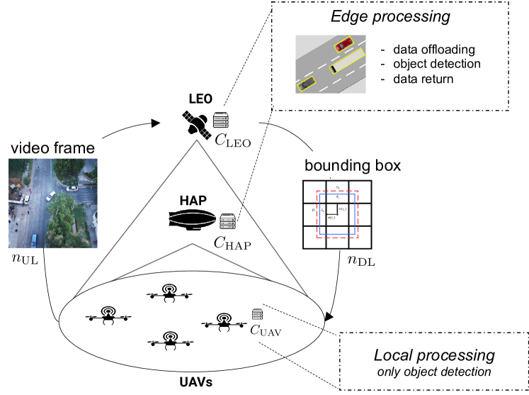
Fig. 1: The edge computing scenario. UAVs are equipped with video cameras recording video frames of size $s_{\rm UL}$ at rate $r$, that may or may not be offloaded to a HAP or a LEO satellite for processing. The processed output is of size $s_{\rm DL}$. The computational capacity is $C_{i}$, $i\in{\{\text{UAV, HAP, LEO}\}}$.

II System Model

In this section we present our research problem (Sec. II-A), and our channel (Sec. II-B) and delay (Sec. II-C) models.

II-A Problem Formulation

We consider a set of $n$ UAVs equipped with video cameras that record video frames of size $s_{\rm UL}$ at an average frame rate $r$. Eventually, video frames have to be processed by an object detection algorithm to detect and recognize critical entities in the surrounding environment, which results in a constant computational load $C_{l}$, expressed in Giga Floating Point Operations (GFLOP), which counts the number of floating point operations required to complete a processing task. The processed output (in this study, the bounding boxes of the detected entities) is returned in a packet of size $s_{\rm DL}\ll s_{\rm UL}$. As shown in Fig. 1, the area is monitored by an upstream HAP or LEO satellite, which may also act as edge server for the UAVs. Therefore, data processing can be performed either onboard the UAVs (i.e., local processing), or at the HAP or the LEO satellite (i.e., edge computing), or as a combination of the two.

The computational capacity, expressed in GFLOP/s and defined in terms of the number of operations that can be processed in one second, is $C_{i}$, $i\in{\{\text{UAV, HAP, LEO}\}}$, with $C_{\rm UAV}<C_{\rm HAP}<C_{\rm LEO}$ due to energy and space constraints. As such, edge computing is faster, at the expense of a non-negligible communication delay for offloading data from the UAVs to the edge server, and for the processed output to be returned. The offloading factor $\eta$ indicates the probability of a frame being offloaded to the HAP or the LEO satellite for edge computing. Therefore, the average arrival rate for data processing at the edge server is $\eta nr$, while for local processing at each UAV it is $(1-\eta)r$. In this paper, we will evaluate the energy consumption and end-to-end delay for local processing vs. edge computing as a function of $\eta$.

II-B Channel Model

We assume that the UAVs and the HAP or the LEO satellite communicate in the millimeter wave (mmWave) bands, and the channel is modeled based on the 3rd Generation Partnership Project (3GPP) specifications for NTN [15, 16]. Assuming an interference-free scenario with UAVs operating in orthogonal frequency bands, the Signal-to-Noise Ratio (SNR) between the UAV and receiver $i\in\{\text{HAP, LEO}\}$ is

$$\gamma_{i}=\frac{\text{EIRP}\cdot({G}/{T})_{i}}{\text{PL}_{i}\cdot K_{b}\cdot B},\>i\in\{\text{HAP, LEO}\}$$ (1)

where EIRP is the effective isotropic radiated power, $({G}/{T})_{i}$ is the receiver antenna-gain-to-noise-temperature, $\text{PL}_{i}$ is the path loss, $K_{b}$ is the Boltzmann constant, and $B$ is the bandwidth. The path loss depends on the carrier frequency and the distance between transmitter and receiver, and accounts for additional atmospheric losses such as scintillation as described in [16].

The ergodic (Shannon) capacity $R_{i}$ can be derived as

$$R_{i}=B\log_{2}(1+\gamma_{i}),\>i\in\{\text{HAP, LEO}\}$$ (2)

II-C End-to-End Delay Model

The system is modeled as a set of D/M/1 queues. At each UAV, the arrival rate is a function of the offloading factor $\eta$ and is equal to $\lambda_{\rm UAV}=(1-\eta)r$, while the service rate is $\mu_{\rm UAV}=C_{\rm UAV}/C_{l}$. At the HAP/LEO edge server, the arrival rate is equal to $\lambda_{i}=\eta rn$ frames/s, while the service rate is $\mu_{i}=C_{i}/C_{l}$ frames/s, $i\in\{\text{HAP, LEO}\}$. According to [17], the average system time (the sum of waiting and service times) for a D/M/1 queue with arrival rate $\lambda$ and service rate $\mu$ is

$$t_{s}(\lambda,\mu)=\frac{1}{\mu(1-\delta)},$$ (3)

where $\delta$ is the root of the equation $\delta=e^{-\mu/\lambda(1-\delta)}$, to be solved numerically. We distinguish between local processing and edge computing.

• Local processing. The end-to-end delay is only due to data processing, and can be computed as

  $$\bar{t}_{\rm UAV}=t_{s}(\lambda_{\rm UAV},\mu_{\rm UAV}).$$ (4)

• Edge computing. The end-to-end delay is the sum of the delay to offload video frames from the UAV to the edge server, the delay for data processing, and the delay for the processed output to be returned to the UAV, i.e.,

  $$\bar{t}_{i}=2\tau^{i}_{p}+t_{\rm UL}^{i}+t_{\rm DL}^{i}+t_{s}(\lambda_{i},\mu_{i}),\>i\in\{\text{HAP, LEO}\}.$$ (5)

  In Eq. 5, $\tau^{i}_{p}=d_{i}/c$ is the propagation delay, where $d_{i}$ is the distance between the UAV and the edge server $i\in\{\text{HAP, LEO}\}$, and $c$ is the speed of light. Moreover, $t_{\rm UL}^{i}$ and $t_{\rm DL}^{i}$ are the transmission delays to send frames to the edge server and to receive the processed output, respectively, so

  $$t_{k}^{i}={s_{k}}/{R_{i}},\>\>k\in\{\text{UL, DL}\},\>i\in\{\text{HAP, LEO}\}.$$ (6)

  It is important to note that the distance between the swarm of UAVs and the LEO satellite is not constant, but varies depending on the elevation angle $\alpha$ as

  $$d_{\rm LEO}(\alpha)=\sqrt{R_{E}^{2}\sin{{}^{2}\alpha}+h^{2}+2hR_{E}}-R_{E}\sin{\alpha},$$ (7)

  where $R_{E}$ is the radius of the Earth, and $h$ is the altitude of the satellite orbit [18].

With an offloading factor $\eta$, which represents the probability of a frame being offloaded to the edge server (either the HAP or the LEO satellite), the average end-to-end delay is

$$\bar{T}=(1-\eta)\bar{t}_{\rm UAV}+\eta\bar{t}_{i},\>i\in\{\text{HAP, LEO}\}.$$ (8)

III Energy Model

In this section we present our energy model to characterize the energy consumption of the UAVs, HAP, and LEO satellite. Specifically, we distinguish between energy for movement (Sec. III-A), data offloading (Sec. III-B), and data processing (Sec. III-C), while the overall energy consumption is given in Sec. III-D. Moreover, in Sec. III-E we describe the energy capacity at the different nodes.

III-A Energy for Movement ($E_{\rm M}$)

We assume that the LEO satellite and the HAP do not consume energy to move, despite some wind and/or air resistance, i.e., $E^{\rm HAP}_{\rm M}=E^{\rm LEO}_{\rm M}=0$, while instead the UAV incurs a significant energy cost for hovering (i.e., controlling and maintaining the UAV in the air). The latter is characterized by the model in [19], which is based on empirical data. So, the hovering power can be written as

$$P^{\rm UAV}_{\rm M}=\sqrt{{\left(mg\right)^{3}}/({2\pi\xi^{2}\psi})},$$ (9)

where $m$ is the mass of the UAV, $g$ is the gravitational acceleration, $\xi$ is the radius of a propeller, and $\psi$ is the air density. Finally, the energy consumption for hovering becomes

$$E^{\rm UAV}_{\rm M}=P^{\rm UAV}_{\rm M}t_{f},$$ (10)

where $t_{f}$ represents the total flying time.

III-B Energy for Data Offloading ($E_{\rm DO}$)

Assuming transmissions in the mmWave spectrum, the energy consumption for data offloading to/from the UAV is modeled based on the analysis in [20]. The energy consumption depends on the type of antenna that is used to transmit or receive data. We distinguish between Uniform Planar Array (UPA) and Circular Aperture Reflector (CAR) antennas.

• UPA antennas. Assuming analog beamforming with $N$ antenna elements, the power consumption to transmit data (i.e., video frames from the UAV to the HAP/LEO, or the processed output from the HAP/LEO to the UAV) is

  where $P_{t}$ is the transmit power, $\zeta\leq 1$ is the efficiency of the power amplifier, and the second term accounts for the power consumption of the circuitry. Specifically, $P_{\rm PS}$, $P_{\rm HPA}$, $P_{\rm DAC}$, $P_{\rm UC}$, and $P_{\rm C}$ are the power consumptions of phase shifters, high-power amplifiers, the digital-to-analog converter, the up-conversion stage, and the combiner. In  Eq. 11 we neglect the power to generate the precoder, which accounts for no more than $5\%$ of the total power consumption [20].

  The power consumption to receive data is

  $$P^{\rm UPA}_{\rm RX}=N(P_{\rm PS}+P_{\rm LNA})+P_{\rm ADC}+P_{\rm DC}+P_{\rm C},$$ (12)

  where $P_{\rm LNA}$, $P_{\rm ADC}$, and $P_{\rm DC}$ are the power consumptions of low-noise amplifiers, the analog-to-digital converter, and the down-conversion stage.

• CAR antennas. The power consumption to transmit and receive data is given by

  $$P^{\rm CAR}_{\rm TX}=\frac{P_{t}}{\zeta}+\Big{(}P_{\rm HPA}+P_{\rm DAC}+P_{\rm UC}+P_{\rm C}\Big{)};$$ (13a)

  $$P^{\rm CAR}_{\rm RX}=P_{\rm LNA}+P_{\rm ADC}+P_{\rm DC}+P_{\rm C}.$$ (13b)

In uplink, the UAV acts as a transmitter and the HAP/LEO as a receiver, while in downlink it is the contrary. Therefore, the total energy consumption for data offloading is

$$E_{\text{DO}}^{\text{UAV}} =t^{i}_{\rm UL}P^{z}_{\rm TX}+t^{i}_{\rm DL}P^{z}_{\rm RX},$$ (14a)

$$E_{\text{DO}}^{i} =t^{i}_{\rm DL}P^{z}_{\rm TX}+t^{i}_{\rm UL}P^{z}_{\rm RX},\>i\in\{\text{HAP, LEO}\},$$ (14b)

where $z\in\{\text{UPA, CAR}\},$ and $t^{i}_{\rm UL}$ and $t^{i}_{\rm DL}$ are the transmission delays to send video frames from the UAV to the HAP/LEO, and the processed output (bounding boxes) from the HAP/LEO to the UAV, respectively, as expressed in Eq. 6.

TABLE I: System parameters.

Layer	UAV	HAP	LEO	Other Parameters
GPU Energy efficiency ($\nu$) [GFLOP/J]	[30,90]	200	200	Computational load ($C_{l}$) [GFLOP]	90
Battery capacity ($E_{b}$) [Wh]	130	8000	6000	Number of UAVs ($n$)	[5,50]
Solar panel area ($S$) [m2]	N/A	100	30	Frame rate ($r$) [fps]	[1,19]
UPA antenna elements ($N$)	[4,128]	64	N/A†	Transmitted power ($P_{t}$) [dBm]	30
Effective isotropic radiated power (EIRP) [dB]	$10\log_{10}(N)-6$	12	32.5	Hovering power ($P^{\rm UAV}_{M}$) [W]	$\sim 212$
Antenna-gain-to-noise-temperature ($G/T$) [dB]	$10\log_{10}(N)-31$	$-13$	13	Radius of the Earth ($R_{E}$) [km]	6371
Altitude ($h$) [km]	0.1	20	600	Boltzmann constant ($K_{b}$) [J/K]	$1.38\cdot 10^{-23}$
Computational capacity ($C$) [GFLOP/s]	1000	20000	20000	UL payload ($s_{\rm UL}$) [Mb]	3
Photovoltaic efficiency ($\chi$)	N/A	0.15	0.15	DL payload ($s_{\rm DL}$) [Mb]	0.1
Extra-terrestrial solar irradiance density ($I$) [W/m2]	N/A	600	600	Bandwidth ($B$) [MHz]	$B_{T}/n=400/n$
†According to [18], LEO satellites use a CAR antenna for communication.

III-C Energy for Data Processing ($E_{\rm P}$)

The energy consumption to process (i.e., perform object detection on) a video frame can be calculated as

$$E_{\rm P}^{i}={C_{l}}/{\nu_{i}},\>i\in\{\rm UAV,HAP,LEO\},$$ (15)

where $C_{l}$ is the constant computational load required to process each video frame in GFLOP, and $\nu_{i}$ is the energy efficiency of the Graphics Processing Unit (GPU) installed at node $i$, expressed in GFLOP/J. Given energy and space constraints, only low-cost GPUs can be installed onboard the UAVs, while the HAP and the LEO satellite can be equipped with more powerful and advanced, so more efficient, GPUs, i.e., $\nu_{\rm LEO}>\nu_{\rm HAP}>\nu_{\text{UAV}}$. This means that the same processing task will consume more energy if it is performed onboard the UAV than at an edge server.

III-D Overall Energy Consumption

Given an offloading factor $\eta$, the overall average energy consumption of a UAV is due to the energy for movement/hovering ($E^{\rm UAV}_{\rm M}$), the energy for on board processing ($E_{P}^{\rm UAV}$, with probability $1-\eta$), and the energy to transmit data frames to the edge server and receive the processed output ($E_{\text{DO}}^{\text{UAV}}$, with probability $\eta$). The overall average energy consumption of a HAP/LEO serving a swarm of $n$ UAVs, with probability $\eta$, is due to the energy for data processing ($E_{\rm P}^{i}$) and the energy to receive data frames and transmit the processed output ($E_{\text{DO}}^{i}$), with $i\in\{\text{HAP, LEO}\}$. Therefore:

$$E_{\rm UAV}(\eta)=\left[(1-\eta)E_{P}^{\rm UAV}+\eta E_{\text{DO}}^{\text{UAV}}\right]rt_{f}+E^{\rm UAV}_{\rm M};$$ (16a)

$$E_{i}(\eta)=\eta rn\left(E_{\rm P}^{i}+E_{\text{DO}}^{i}\right)t_{f},\>i\in\{\text{HAP, LEO}\}.$$ (16b)

III-E Energy Capacity ($E_{C}$)

Both the UAVs and the HAP/LEO edge server have energy constraints, so it is important to model the actual energy capacity, i.e., the energy available at the nodes, in order to understand the impact of the offloading and processing operations on the energy consumption. For the UAV, the energy capacity is equal to the energy stored in the batteries, while the HAP and the LEO satellite can additionally harvest energy from solar panels, i.e.,

$$E_{C}^{\rm UAV}=E_{b}^{\rm UAV};$$ (17a)

$$E_{C}^{i}=E_{b}^{i}+E_{h}^{i},\>i\in\{\text{HAP, LEO}\},$$ (17b)

where $E_{b}$ is the capacity of the batteries, and $E_{h}$ is the energy harvested from the solar panels. Specifically, $E_{h}$ is a function of the efficiency of the photovoltaic system ($\chi$), the total extra-terrestrial solar irradiance density on the surface of node ($I$), the total area of the solar panels installed on node ($S$) [21], and the flying time ($t_{f}$), and takes into account the fact that all the energy that could be harvested when the battery is full cannot be stored and is therefore lost.

(a) Stability for $\eta=0$.

(b) Stability for $\eta=0.5$.

(c) Stability for $\eta=1$.

Fig. 2: Stability of the D/M/1 queues as a function of the frame rate $r$, the number of UAVs $n$, and the offloading factor $\eta$.

(a) $\nu_{\rm UAV}=50$ GFLOP/J, $n=20$, and $r=10$ fps.

(b) $N=8$, $\nu_{\rm UAV}=50$ GFLOP/J, and $n=15$.

(c) $N=8$, and $n=20$, and $r=10$ fps.

(d) $N=8$, $\nu_{\rm UAV}=50$ GFLOP/J, and $r=10$ fps.

Fig. 3: HAP-assisted edge computing. Average UAV autonomy $\bar{\kappa}$ (left) and average delay $\bar{T}$ (right) vs. $\eta$, as a function of the number of antenna elements $N$ at the UAV, the energy efficiency $\nu_{\rm UAV}$ of the GPUs at the UAV, the number of UAVs $n$, and the frame rate $r$.

IV Performance Evaluation

In Sec. IV-A we introduce our simulation setup, in Secs. IV-B and IV-C we present our results for HAP- and LEO-assisted edge computing, respectively, and in Sec. IV-D we evaluate the energy consumption of the edge server.

IV-A Simulation Setup and Parameters

Our main simulation parameters are summarized in Table I.

Communication parameters. Communication is in the mmWave spectrum, specifically in the Ka-bands at 30 (20) GHz in uplink (downlink) [18]. The total bandwidth is $B_{\rm T}=400$ MHz, and the UAVs operate in orthogonal frequency bands, so the actual bandwidth available to each UAV is $B=B_{\rm T}/n$. According to [18], LEO satellites communicate using a CAR antenna, whereas the HAP is equipped with a UPA antenna with $N=64$ elements. UAVs also operate with a UPA antenna, and we vary the value of $N$ from 4 to 128.

Energy parameters. The battery capacity of a UAV is $E^{\rm UAV}_{b}=130$ Wh, equivalent to that of a DJI Matrice 100 [22]. Regarding the hovering, from the model in [19] we have that $m=3$ kg, $\xi=0.3$ m, and $\psi=1$ kg/m³, so the power consumption in Eq. 9 is around 200 W. The HAP and LEO satellite are powered by batteries with a total capacity of $E^{\rm HAP}_{b}=8$ kWh and $E^{\rm LEO}_{b}=6$ kWh, respectively. As the HAP and the LEO satellite operate above the stratosphere, they can also harvest energy from solar panels of $S_{\rm HAP}=100$ m² and $S_{\rm LEO}=30$ m², respectively.

Our scenario consists of a set of $n$ UAVs that capture images of size $s_{\rm UL}=3$ Mb [23] at a frame rate $r$, while the processed output, in the form of bounding boxes, is of size $s_{\rm UL}=0.1$ Mb. We assume that all the frames require the same computational load $C_{l}=90$ GFLOP [24]. UAVs operate with low-cost GPUs (e.g., a Jetson TX2 GPU), so we set the energy efficiency $\nu_{\rm UAV}$ in the range $[30,90]$ GFLOP/J, while the computational capacity is $C_{\rm UAV}=1000$ GFLOP/s. On the contrary, the HAP and the LEO satellite can support high-performance GPUs with a higher energy efficiency of $\nu_{\rm HAP}=\nu_{\rm LEO}=200$ GFLOP/J, and a computational capacity of $C_{\rm HAP}=C_{\rm LEO}=20000$ GFLOP/s.

As far as data offloading is concerned (see Sec. III-B), using the parameters in [20, 26], the total power consumption to transmit and receive data in case of a UPA antenna with $N$ elements is $P^{\rm UPA}_{\rm TX}=P_{t}+168N+178.5$ mW (with $P_{t}=30$ dBm) and $P^{\rm UPA}_{\rm RX}=69N+266.8$ mW, respectively, while in case of a CAR antenna we have $P^{\rm CAR}_{\rm TX}=316$ mW and $P^{\rm CAR}_{\rm RX}=305.8$ mW, respectively.

Performance metrics. We evaluate:

• the average delay $\bar{T}$, measured as in Eq. (8);

• the average UAV autonomy $\bar{\kappa}$, measured as the ratio between the energy consumption for hovering, i.e., $E^{\rm UAV}_{\rm M}$ in Eq. 10, and the overall energy consumption of the UAV, i.e., $E_{\rm UAV}$ in Eq. 16a. As $\bar{\kappa}$ approaches $1$, the energy consumption is dominated by the sole energy for hovering, which promotes better autonomy;

• the energy consumption at the edge server, i.e., $E_{\rm HAP}$ and $E_{\rm LEO}$ in Eq. 16b.

Simulation results are given as a function of the offloading factor $\eta$. We consider: (i) local processing with $\eta=0$, where the processing is done onboard the UAVs; (ii) edge computing with $\eta=0.5$, where, on average, half of the frames are processed locally onboard the UAVs and the rest is offloaded to the edge server; and (iii) edge computing with $\eta=1$, where all the frames are offloaded to the edge server. Moreover, we investigate the impact of the frame rate $r$, the number of antenna elements $N$ at the UAV, the energy efficiency $\nu_{\rm UAV}$ of the GPUs at the UAV, the elevation angle $\alpha$ of the LEO satellite, the total flying time $t_{f}$, and the number of UAVs $n$. Notably, to maintain the stability of the D/M/1 queues (see Sec. II-C), the load factor $\rho=\lambda/\mu$ must be less than 1. This sets a limit on the maximum number of UAVs and the frame rate that the network can handle. For example, Fig. 2(a) illustrates that the maximum frame rate to maintain stability in case of local processing (i.e., $\eta=0$) is 10 fps, while it is 20 fps if $\eta=0.5$ given that the burden of data processing is partially delegated to the edge server. Moreover, in Figs. 2(b) and 2(c) we report the load factor $\rho$ vs. $n$ and $r$, which can be used to determine the range of values where stability is guaranteed, i.e., $\rho<1$. For instance, when $\eta=0.5$ the network can support up to $20$ UAVs with $r=20$ fps. In turn, when $\eta=1$, the edge server becomes more congested, and can support only up to $10$ UAVs with $r=20$ fps.

(a) $\alpha=70^{\circ}$, and $n=20$.

(b) $\alpha=70^{\circ}$, and $n=20$.

(c) $N=64$, and $n=20$.

(d) $N=64$, and $n=20$.

Fig. 4: LEO-assisted edge computing. Average UAV autonomy $\bar{\kappa}$ (left) and average delay $\bar{T}$ (right) vs. $\eta$, as a function of the elevation angle $\alpha$ of the LEO satellite, and the number of antenna elements $N$ of the UAV.

IV-B HAP-Assisted Edge Computing

In this section we evaluate the performance of HAP-assisted edge computing vs. local processing. As expected, Fig. 3 shows that data offloading can generally improve the UAV autonomy, but at the expense of a higher delay. Notably, the impact of $N$ is non-linear, as illustrated in Fig. 3(a). At first, the UAV autonomy increases as $N$ increases. In fact, the antenna gain produced by beamforming grows with $N$, which permits to improve the quality of the channel and transmit data faster, thereby reducing the energy consumption for data offloading as per Eq. 14a. Then, as $N>16$, the power consumption of the circuitry, which is proportional to $N$ as per Eq. 11, keeps increasing but with limited channel improvements, which leads to performance degradation, e.g., for $\eta=1$, the autonomy $\bar{\kappa}$ decreases from 97% to 93% as $N$ grows from 16 to 128.

In Fig. 3(b) we plot the average delay as a function of the frame rate $r$. We observe that local processing, which does not involve additional delays for data transmission to the edge server, is the most desirable option as long as $r<7$ fps: the average delay is between 150 and 200 ms. Then, for $r>10$ fps, the system becomes unstable. In this case, (partial) data offloading can improve the queuing delay by delegating some processing tasks to the HAP server, despite the communication overhead for uploading data frames. In particular, the delay is less than 200 ms in most configurations for $\eta=0.5$, and around 250 ms for $\eta=1$.

Notice that the energy consumption for local processing depends on the energy efficiency of the GPUs installed at the UAVs. In Fig. 3(c) we see that using more powerful and efficient (though more expensive) GPUs can reduce the energy consumption for data processing and increase the UAV autonomy by up to $10\%$. Notably, for $\nu_{\rm UAV}=90$ GFLOP/J, $\bar{\kappa}$ is as high as 95%.

In Fig. 3(d) we see that local processing requires around $450$ ms for each video frame when $N=8$ and $r=10$ fps, regardless of the value of $n$. On the contrary, the average delay for edge computing via the HAP grows with $n$ due to the more frequent offloading requests to the edge server, and the resulting more populated queues as the number of UAVs increases. In particular, the system becomes unstable as $n\geq 20$ for $\eta=1$, and as $n\geq 40$ for $\eta=0.5$, which is consistent with the results in Fig. 2.

IV-C LEO-Assisted Edge Computing

In this section we evaluate the performance of LEO-assisted edge computing vs. local processing. In general, the delay for data offloading is significantly higher than HAP-assisted edge computing given the longer communication distance to the LEO satellite and the resulting higher path loss. For example, in Fig. 4 we see that the delay for $\eta=1$ can be even higher than 1 s, which is not compatible with the requirements of most wireless applications [1]. In this scenario, local processing becomes the most convenient choice in terms of both energy consumption (or UAV autonomy) and delay, especially when $N<4$. As $N$ increases, the beamforming gain also increases, and the channel quality between the UAV and the LEO satellite improves accordingly. Specifically, the average delay for edge computing for $\eta=1$ decreases from 1120 to only 100 ms when $N$ grows from 4 to 128 elements, with almost no degradation in terms of UAV autonomy, despite the higher power consumption of the circuitry as the number of antennas increases. LEO-assisted edge computing outperforms local processing in terms of both energy consumption (Fig. 4(a)) and delay (Fig. 4(b)) as $N>16$ (8) for $\eta=1$ (0.5).

Notice that the offloading performance is affected by the elevation angle $\alpha$ between the UAVs and the LEO satellite, as depicted in Figs. 4(c) and 4(d). In particular, as $\alpha$ decreases the path loss increases due to the resulting longer distance between the two endpoints, leading to a higher transmission delay. For example, for $\alpha=10^{\circ}$ the UAV autonomy for edge computing ($\eta=1$) is only 60%, vs. more than 80% for local processing. Edge computing becomes more convenient than local processing when $\alpha\geq 30^{\circ}$ in terms of delay, and $\geq 50^{\circ}$ in terms of both UAV autonomy and delay.

(a)

Fig. 5: Energy consumption $E_{\rm HAP}$ (plain bar) and $E_{\rm LEO}$ (striped bar) of the edge server for HAP- and LEO-assisted edge computing, respectively, vs. the total flying time $t_{f}$, as a function of the number of UAVs $n$.

IV-D Energy Consumption at the Edge Server

In order to evaluate the impact of data offloading, in Fig. 5 we show the energy consumption $E_{i}$ at the edge server $i\in\{\text{HAP, LEO}\}$ as a function of $n$. We see that the energy consumption at the LEO satellite is lower than at the HAP since the former uses CAR antennas instead of UPA antennas, which reduces the energy consumption for data transmission and reception (by up to $60\%$ when $n=20$). As expected, the energy consumption grows over time, and as the number of UAVs increases. For example, for $n=5$ the LEO satellite (HAP) consumes only 24 (50) Wh after 1 hour of service, while for $n=20$ the energy consumption is more than 4 times higher, given that the edge server has to process more incoming requests. This may saturate the available capacity, which motivates our research towards the optimal offloading factor and configuration for edge computing.

V Conclusions and Future Works

In this work, we explored the feasibility of HAP- and LEO-assisted edge computing as a solution to process UAV data. We evaluated the energy consumption and the delay for data processing considering onboard processing vs. processing at the HAP or the LEO satellite. We showed that (partial) HAP-assisted edge computing can improve both autonomy and delay compared to onboard processing in many configurations, and especially when the number of UAVs is lower than 40, and the frame rate is higher than 7 fps. In turn, LEO-assisted edge computing works well only using directional antennas at the UAVs, and with an elevation angle of at least $50^{\circ}$.

In our future research, we will formalize an optimization problem with both energy consumption and delay constraints, to identify the optimal offloading factor for edge computing.

References

- [1] M. Giordani, M. Polese, M. Mezzavilla, S. Rangan, and M. Zorzi, “Toward 6G Networks: Use Cases and Technologies,” IEEE Commun. Mag., vol. 58, no. 3, pp. 55–61, March 2020.
- [2] M. Giordani and M. Zorzi, “Non-Terrestrial Networks in the 6G Era: Challenges and Opportunities,” IEEE Network, vol. 35, no. 2, pp. 244–251, Dec. 2021.
- [3] P. Chandhar and E. G. Larsson, “Massive MIMO for Connectivity With Drones: Case Studies and Future Directions,” IEEE Access, vol. 7, pp. 94 676–94 691, Jul. 2019.
- [4] B. H. Y. Alsalam, K. Morton, D. Campbell, and F. Gonzalez, “Autonomous UAV with vision based on-board decision making for remote sensing and precision agriculture,” in IEEE Aerospace Conference, 2017.
- [5] S. Zhang, H. Zhang, and L. Song, “Beyond D2D: Full Dimension UAV-to-Everything Communications in 6G,” IEEE Transactions on Vehicular Technology, vol. 69, no. 6, pp. 6592–6602, Apr. 2020.
- [6] M. Bordin, M. Giordani, M. Polese, T. Melodia, and M. Zorzi, “Autonomous Driving From the Sky: Design and End-to-End Performance Evaluation,” in IEEE Globecom Workshops (GC Wkshps), 2022.
- [7] W. Z. Khan, E. Ahmed, S. Hakak, I. Yaqoob, and A. Ahmed, “Edge computing: A survey,” Future Generation Computer Systems, vol. 97, pp. 219–235, Aug. 2019.
- [8] K. Kim and C. S. Hong, “Optimal Task-UAV-Edge Matching for Computation Offloading in UAV Assisted Mobile Edge Computing,” in Asia-Pacific Network Operations and Management Symposium (APNOMS), 2019.
- [9] A. Traspadini, M. Giordani, and M. Zorzi, “UAV/HAP-Assisted Vehicular Edge Computing in 6G: Where and What to Offload?” Joint European Conference on Networks and Communications & 6G Summit (EuCNC/6G Summit), 2022.
- [10] A. Chaoub, M. Giordani, B. Lall, V. Bhatia, A. Kliks, L. Mendes, K. Rabie, H. Saarnisaari, A. Singhal, N. Zhang, S. Dixit, and M. Zorzi, “6G for Bridging the Digital Divide: Wireless Connectivity to Remote Areas,” IEEE Wireless Commun., pp. 160–168, July 2021.
- [11] C. Liu, W. Feng, X. Tao, and N. Ge, “MEC-Empowered Non-Terrestrial Network for 6G Wide-Area Time-Sensitive Internet of Things,” Engineering, vol. 8, pp. 96–107, Jan. 2022.
- [12] A. Traspadini, M. Giordani, G. Giambene, and M. Zorzi, “Real-Time HAP-Assisted Vehicular Edge Computing for Rural Areas,” IEEE Wireless Communications Letters, vol. 12, no. 4, pp. 674–678, Apr. 2023.
- [13] D. Wang, A. Traspadini, M. Giordani, M.-S. Alouini, and M. Zorzi, “On the Performance of Non-Terrestrial Networks to Support the Internet of Things,” Asilomar Conference on Signals, Systems, and Computers, 2022.
- [14] Y. Chen, B. Ai, Y. Niu, H. Zhang, and Z. Han, “Energy-Constrained Computation Offloading in Space-Air-Ground Integrated Networks Using Distributionally Robust Optimization,” IEEE Transactions on Vehicular Technology, vol. 70, no. 11, pp. 12 113–12 125, Nov. 2021.
- [15] 3GPP, “Solutions for NR to support Non-Terrestrial Networks (NTN),” TR 38.821 (Release 16), 2020.
- [16] M. Giordani and M. Zorzi, “Satellite Communication at Millimeter Waves: a Key Enabler of the 6G Era,” IEEE International Conference on Computing, Networking and Communications (ICNC), 2020.
- [17] B. Jansson, “Choosing a Good Appointment System-A Study of Queues of the Type (D/M/1),” Operations Research, vol. 14, no. 2, pp. 292–312, Mar./Apr. 1966.
- [18] 3GPP, “Study on New Radio (NR) to support non terrestrial networks,” TR 38.811 (Release 15), 2018.
- [19] H. V. Abeywickrama, B. A. Jayawickrama, Y. He, and E. Dutkiewicz, “Comprehensive Energy Consumption Model for Unmanned Aerial Vehicles, Based on Empirical Studies of Battery Performance,” IEEE Access, vol. 6, pp. 58 383–58 394, Oct. 2018.
- [20] A. Pizzo and L. Sanguinetti, “Optimal design of energy-efficient millimeter wave hybrid transceivers for wireless backhaul,” in 15th International Symposium on Modeling and Optimization in Mobile, Ad Hoc, and Wireless Networks (WiOpt), 2017.
- [21] S. C. Arum, D. Grace, P. D. Mitchell, M. D. Zakaria, and N. Morozs, “Energy Management of Solar-Powered Aircraft-Based High Altitude Platform for Wireless Communications,” Electronics, vol. 9, no. 1, Jan. 2020.
- [22] W. Woźniak and M. Jessa, “Selection of solar powered unmanned aerial vehicles for a long range data acquisition chain,” Sensors, vol. 21, no. 8, Apr. 2021.
- [23] P. Testolina, F. Barbato, U. Michieli, M. Giordani, P. Zanuttigh, and M. Zorzi, “SELMA: SEmantic Large-Scale Multimodal Acquisitions in Variable Weather, Daytime and Viewpoints,” IEEE Transactions on Intelligent Transportation Systems, vol. 24, no. 7, pp. 7012–7024, Mar. 2023.
- [24] Z. Saeed, M. H. Yousaf, R. Ahmed, S. A. Velastin, and S. Viriri, “On-Board Small-Scale Object Detection for Unmanned Aerial Vehicles (UAVs),” Drones, vol. 7, no. 5, May 2023.
- [25] A. Biddulph, T. Houliston, A. Mendes, and S. K. Chalup, “Comparing Computing Platforms for Deep Learning on a Humanoid Robot,” Neural Information Processing, 2018.
- [26] P. Skrimponis, S. Dutta, M. Mezzavilla, S. Rangan, S. H. Mirfarshbafan, C. Studer, J. Buckwalter, and M. Rodwell, “Power Consumption Analysis for Mobile MmWave and Sub-THz Receivers,” in 6G Wireless Summit, 2020.