Questions of flavor physics and neutrino mass from a flipped hypercharge

Abstract

The flavor structure of quarks and leptons is not yet fully understood, but it hints a more fundamental theory of non-universal generations. We therefore propose a simple extension of the Standard Model by flipping (i.e., enlarging) the hypercharge $U(1)_{Y}$ to $U(1)_{X}\otimes U(1)_{N}$ for which both $X$ and $N$ depend on generations of both quark and lepton. By anomaly cancellation, this extension not only explains the existence of just three fermion generations as observed but also requires the presence of a right-handed neutrino per generation, which motivates seesaw neutrino mass generation. Furthermore, in its minimal version with a scalar doublet and two scalar singlets, the model naturally generates the measured fermion-mixing matrices while it successfully accommodates several flavor anomalies observed in the neutral meson mixings, $B$-meson decays, lepton-flavor-violating decays of charged leptons, as well as satisfying constraints from particle colliders.

I Introduction

Although the Standard Model (SM) has been highly successful in describing observed phenomena, it leaves many striking features of the physics of our world unexplained. This work would focus on the issues relating to the number of fermion generations, the generation of neutrino masses, fermion mass hierarchies, and flavor mixing profiles [1].

In the SM, the electroweak symmetry reveals a partial unification of weak and electromagnetic interactions, which is based upon the non-Abelian gauge group $SU(2)_{L}\otimes U(1)_{Y}$, where $Y$ is an Abelian charge, well known as hypercharge [2, 3, 4, 5]. The electric charge operator takes the form $Q=T_{3}+Y$, in which $T_{3}$ is the third component of the $SU(2)_{L}$ weak isospin. The value of $T_{3}$ is quantized due to the non-Abelian nature of $SU(2)_{L}$, whereas in contrast the value of $Y$ is entirely arbitrary on the theoretical ground, because the Abelian $U(1)_{Y}$ algebra is trivial. Indeed, the hypercharge is often chosen to describe observed electric charges, while it does not explain them. An interesting question relating to the nature of the SM hypercharge is whether the conventional choice of generation-universal hypercharge causes the SM to be unable to address the issues. The present work does not directly answer this question. Instead of that, we look for an extension of $U(1)_{Y}$ to generation-dependent Abelian factors, as general, which naturally solves the issues.

For this aim, we embed $U(1)_{Y}$ in $U(1)_{X}\otimes U(1)_{N}$ for which both $X$ and $N$ are generation-dependent but determining $Y=X+N$, as observed. It is clear that $X,N$ may be an intermediate new physics phase resulting from a GUT and/or string breaking. Additionally, anomaly cancellation fixes both the number of fermion generations and values of $X,N$. Interestingly, we find for the first time that both quark and lepton generations are not universal under a gauge charge as of $X,N$. We investigate the model with a minimal scalar content in detail, which is responsible for the small, nonzero neutrino masses [6, 7], the measured fermion-mixing matrices [1, 8], and several flavor-physics anomalies, such as mass splittings in $K$- and $B$-meson systems [1, 9], $B$-meson decays [9, 10], and lepton-flavor-violating (LFV) decays of charged leptons [1, 11, 12, 13].

Let us remind the reader concering the two features of the present work. First, we argue that the number of fermion generations is precisely three, as observed, which comes only from anomaly cancellation. This is quite different from the 3-3-1 model [14, 15, 16, 17, 18, 19, 20, 21, 22] as well as our previous proposals [23, 24, 25, 26], in which anomaly cancellation implies that the fermion generation number is an integer multiple of three, and then it is necessary to add the QCD asymptotic freedom condition to get the number of fermion generations equal to three. Second, in the present work, we consider the possibility that the first lepton generation (the third quark generation) carries Abelian charges different from the remaining lepton (quark) generations under the new gauge groups, $U(1)_{X}\otimes U(1)_{N}$. Consequently, the fermion-mixing matrices are recovered, appropriate to experiment [1, 8], because necessary small mixings arise only from nonrenormalizable operators. Interestingly enough, flavor-changing neutral currents (FCNCs) appear at the tree level in both the quark and lepton sectors.

The rest of this work is organized as follows. We present the new model in Sec. II. We investigate the fermion mass spectra in Sec. III. We diagonalize the gauge and scalar sectors in Sec. IV to identify physical fields. We determine the interactions of fermions and gauge bosons in Sec. V. We examine flavor physics observables and compare them to experimental results in Sec. VI. We discuss the collider bounds in Sec. VII. Finally, we summarize our results and conclude this work in Sec. VIII.

II The model

II.1 Anomaly cancellation and generation number

As mentioned, the model under consideration is based on gauge symmetry,

$$SU(3)_{C}\otimes SU(2)_{L}\otimes U(1)_{X}\otimes U(1)_{N},$$ (1)

in which the first two factors are exactly those of the SM, whereas the last two factors are flipped (i.e., extended) from the weak hypercharge symmetry $U(1)_{Y}$. The new gauge charges depend on flavors of both quarks and leptons as

$$X = 3z[Bi^{r^{2}(r-1)}+Li^{r(r-1)}],$$ (2)

$$N = Y-X,$$ (3)

where $B(L)$ denotes normal baryon (lepton) number, $Y$ labels the hypercharge, $z$ is an arbitrary non-zero parameter, $i$ is the imaginary unit, and $r$ is a flavor index, $r=1,2,\cdots,N_{f}$. Notice that $X$ is Hermitian, since $i^{r(r-1)}=(-1)^{\frac{r(r-1)}{2}}$ is always real. Additionally, the charges $X$’s of quark and lepton generations determined by Eq. (2) are either the same or opposite in sign, leading to reduced degrees of freedom in the model. The electric charge operator is embedded in the gauge symmetry as

$$Q=T_{3}+X+N$$ (4)

with $T_{n}\,(n=1,2,3)$ are the $SU(2)_{L}$ generators. The SM fermions transform under the gauge symmetry as follows:

$$l_{rL} = \left(\nu_{rL},e_{rL}\right)^{T}\sim\left({\bf 1},{\bf 2},3zi^{r(r-1)},-1/2-3zi^{r(r-1)}\right),$$ (5)

$$e_{rR} \sim \left({\bf 1},{\bf 1},3zi^{r(r-1)},-1-3zi^{r(r-1)}\right),$$ (6)

$$q_{rL} = \left(u_{rL},d_{rL}\right)^{T}\sim\left({\bf 3},{\bf 2},zi^{r^{2}(r-1)},1/6-zi^{r^{2}(r-1)}\right),$$ (7)

$$u_{rR} \sim \left({\bf 3},{\bf 1},zi^{r^{2}(r-1)},2/3-zi^{r^{2}(r-1)}\right),$$ (8)

$$d_{rR} \sim \left({\bf 3},{\bf 1},zi^{r^{2}(r-1)},-1/3-zi^{r^{2}(r-1)}\right).$$ (9)

It is interesting that the charge $X$ defined by Eq. (2) is periodic in $r$ with period 4, i.e., with $r=1,2,3,4,5,6,7,8,\cdots$, then

$$X=z,z,-z,z,z,z,-z,z,\cdots$$ (10)

for the quark generations and

$$X=3z,-3z,-3z,3z,3z,-3z,-3z,3z,\cdots$$ (11)

for the lepton generations. Hence, we express the number of fermion generations as $N_{f}=4x-y$ with $x=1,2,3,\cdots$ and $y=0,1,2,3$. Take an example, $N_{f}=5$ then $x=2$ and $y=3$. Considering the anomaly $[SU(2)_{L}]^{2}U(1)_{X}$, we get

$$[SU(2)_{L}]^{2}U(1)_{X}\sim\sum_{\mathrm{doublets}}X_{f_{L}}=\left\{\begin{array}[]{ll}6z(x-1)&\text{ if }y=1\\ 6zx&\text{ if }y=0,2,3\end{array},\right.$$ (12)

which implies that this anomaly is canceled if and only if $x=y=1$, or equivalently $N_{f}=3$ as observed. Because of lepton and quark generation discrepancies, we conveniently use two kinds of generation indices, such as $\alpha,\beta=1,2$ for the first two quark generations, while $a,b=2,3$ for the last two lepton generations; generically, $n,m=1,2,3$ run over $N_{f}=3$.

With $N_{f}=3$ and the fermion content as in Eqs. (5)–(9), two anomalies $[\text{Gravity}]^{2}U(1)_{X}$ and $[U(1)_{X}]^{3}$ are not canceled yet, namely

$$\left[\text{Gravity}\right]^{2}U(1)_{X} \sim \sum_{\mathrm{fermions}}(X_{f_{L}}-X_{f_{R}})=-3z,$$ (13)

$$\left[U(1)_{X}\right]^{3} \sim \sum_{\mathrm{fermions}}(X^{3}_{f_{L}}-X^{3}_{f_{R}})=-27z^{3}.$$ (14)

To cancel these anomalies, we introduce right-handed neutrinos $\nu_{pR}\sim({\bf 1},{\bf 1},X_{\nu_{pR}},-X_{\nu_{pR}})$ for $p=1,2,\cdots,N_{R}$ into the theory as fundamental constituents, satisfying

$$\sum_{p=1}^{N_{R}}X_{\nu_{pR}}=-3z,\hskip 14.22636pt\sum_{p=1}^{N_{R}}X^{3}_{\nu_{pR}}=-27z^{3}.$$ (15)

Solving the equations in Eq. (15), as well as requiring that at least two right-handed neutrinos to be identically responsible for neutrino mass generation, we obtain a unique nontrivial solution, such as

$$X_{\nu_{1R}}=3z,\hskip 14.22636ptX_{\nu_{aR}}=-3z,$$ (16)

which implies that the resulting right-handed neutrinos have the lepton number as usual.

With presence of the three right-handed neutrinos, whose $X$ charges obey Eq. (16), it is easily checked that the remaining anomalies, including $[SU(3)_{C}]^{2}U(1)_{X}$, $[SU(3)_{C}]^{2}U(1)_{N}$, $[SU(2)_{L}]^{2}U(1)_{N}$, $[\text{Gravity}]^{2}U(1)_{N}$, $[U(1)_{N}]^{3}$, $[U(1)_{X}]^{2}U(1)_{N}$, and $U(1)_{X}[U(1)_{N}]^{2}$, are all canceled, independent of arbitrary $z$.

II.2 Minimal particle content and symmetry breaking

The particle content of the model, including fermions and scalars, as well as their quantum numbers under the gauge symmetry, are listed in Table 1. In addition to the SM fermions, three right-handed neutrinos must be included as fundamental fermions to suppress the anomalies, as shown in the previous subsection. Concerning the scalar sector, we introduce two singlets $\chi_{1,2}$ and a doublet $\phi$ under $SU(2)_{L}$. The singlets $\chi_{1,2}$ are necessarily presented to break $U(1)_{X}\otimes U(1)_{N}$ down to the weak hypercharge symmetry $U(1)_{Y}$, provide the Majorana masses for right-handed neutrinos, and recover the mixing matrices in quark and lepton sectors. Of course, the scalar doublet $\phi$ that is identified to the SM-Higgs doublet must be used to break $SU(2)_{L}\otimes U(1)_{Y}$ down to the electromagnetic symmetry $U(1)_{Q}$ and generate the masses for ordinary charged fermions, as well as Dirac masses for neutrinos.

The scheme of symmetry breaking is given by

$SU(3)_{C}\otimes SU(2)_{L}\otimes U(1)_{X}\otimes U(1)_{N}$

$\downarrow\Lambda_{1,2}$

$SU(3)_{C}\otimes SU(2)_{L}\otimes U(1)_{Y}$

$\downarrow v$

$SU(3)_{C}\otimes U(1)_{Q}$

Here, the scalar fields develop the vacuum expectation values (VEVs), such as

$$\langle\phi\rangle=\begin{pmatrix}0\\ \frac{v}{\sqrt{2}}\end{pmatrix},\hskip 14.22636pt\langle\chi_{1}\rangle=\frac{\Lambda_{1}}{\sqrt{2}},\hskip 14.22636pt\langle\chi_{2}\rangle=\frac{\Lambda_{2}}{\sqrt{2}},$$ (17)

satisfying $v=246\text{ GeV}$ and $\Lambda_{1,2}\gg v$ for consistency with the SM.

Multiplets	$SU(3)_{C}$	$SU(2)_{L}$	$U(1)_{X}$	$U(1)_{N}$
$l_{1L}=(\nu_{1L},e_{1L})^{T}$	$\bf 1$	$\bf 2$	$3z$	$-1/2-3z$
$\nu_{1R}$	$\bf 1$	$\bf 1$	$3z$	$-3z$
$e_{1R}$	$\bf 1$	$\bf 1$	$3z$	$-1-3z$
$l_{aL}=(\nu_{aL},e_{aL})^{T}$	$\bf 1$	$\bf 2$	$-3z$	$-1/2+3z$
$\nu_{aR}$	$\bf 1$	$\bf 1$	$-3z$	$3z$
$e_{aR}$	$\bf 1$	$\bf 1$	$-3z$	$-1+3z$
$q_{\alpha L}=(u_{\alpha L},d_{\alpha L})^{T}$	$\bf 3$	$\bf 2$	$z$	$1/6-z$
$u_{\alpha R}$	$\bf 3$	$\bf 1$	$z$	$2/3-z$
$d_{\alpha R}$	$\bf 3$	$\bf 1$	$z$	$-1/3-z$
$q_{3L}=(u_{3L},d_{3L})^{T}$	$\bf 3$	$\bf 2$	$-z$	$1/6+z$
$u_{3R}$	$\bf 3$	$\bf 1$	$-z$	$2/3+z$
$d_{3R}$	$\bf 3$	$\bf 1$	$-z$	$-1/3+z$
$\phi=(\phi_{1}^{+},\phi_{2}^{0})^{T}$	$\bf 1$	$\bf 2$	$0$	$1/2$
$\chi_{1}$	$\bf 1$	$\bf 1$	$2z$	$-2z$
$\chi_{2}$	$\bf 1$	$\bf 1$	$6z$	$-6z$

Table 1: Matter content in the model, where $\alpha=1,2$ and $a=2,3$ are generation indices, while $z$ is an arbitrarily nonzero parameter.

Notice that the scalar content introduced above is minimal. Alternatively, a generic model can be constructed by introducing two new scalar doublets, namely $\phi^{\prime}\sim({\bf 1},{\bf 2},2z,1/2-2z)$ and $\phi^{\prime\prime}\sim({\bf 1},{\bf 2},6z,1/2-6z)$, in addition to the usual doublet $\phi$. This would produce a complete mixing in the quark and lepton sectors at tree level. Additionally, such a model presents phenomenological aspects of interest to be differently from the current model and should be published elsewhere.

III Fermion mass

The Yukawa Lagrangian for quarks and leptons in the current model is given by

$$\mathcal{L}_{\mathrm{Yukawa}} = y^{d}_{\alpha\beta}\bar{q}_{\alpha L}\phi d_{\beta R}+y^{d}_{33}\bar{q}_{3L}\phi d_{3R}+\frac{y^{d}_{\alpha 3}}{M}\bar{q}_{\alpha L}\phi\chi_{1}d_{3R}+\frac{y^{d}_{3\beta}}{M}\bar{q}_{3L}\phi\chi_{1}^{*}d_{\beta R}$$ (18)

$$+y^{u}_{\alpha\beta}\bar{q}_{\alpha L}\tilde{\phi}u_{\beta R}+y^{u}_{33}\bar{q}_{3L}\tilde{\phi}u_{3R}+\frac{y^{u}_{\alpha 3}}{M}\bar{q}_{\alpha L}\tilde{\phi}\chi_{1}u_{3R}+\frac{y^{u}_{3\beta}}{M}\bar{q}_{3L}\tilde{\phi}\chi_{1}^{*}u_{\beta R}$$

$$+y^{e}_{11}\bar{l}_{1L}\phi e_{1R}+y^{e}_{ab}\bar{l}_{aL}\phi e_{bR}+\frac{y^{e}_{1b}}{M}\bar{l}_{1L}\phi\chi_{2}e_{bR}+\frac{y^{e}_{a1}}{M}\bar{l}_{aL}\phi\chi_{2}^{*}e_{1R}$$

$$+y^{\nu}_{11}\bar{l}_{1L}\tilde{\phi}\nu_{1R}+y^{\nu}_{ab}\bar{l}_{aL}\tilde{\phi}\nu_{bR}+\frac{y^{\nu}_{1b}}{M}\bar{l}_{1L}\tilde{\phi}\chi_{2}\nu_{bR}+\frac{y^{\nu}_{a1}}{M}\bar{l}_{aL}\tilde{\phi}\chi_{2}^{*}\nu_{1R}$$

$$+\frac{1}{2}f^{\nu}_{11}\bar{\nu}^{c}_{1R}\chi_{2}^{*}\nu_{1R}+\frac{1}{2}f^{\nu}_{ab}\bar{\nu}^{c}_{aR}\chi_{2}\nu_{bR}+F^{\nu}_{1b}\bar{\nu}^{c}_{1R}\nu_{bR}+\mathrm{H.c.},$$

where $\tilde{\phi}=i\sigma_{2}\phi^{*}$ with $\sigma_{2}$ is the second Pauli matrix, $M$ is a new physics scale that defines the effective interactions, and the couplings $y$ and $f$ are dimensionless. The bare mass $F$ connects $\nu_{1R}$ and $\nu_{2,3R}$, possibly obtaining a value ranging from zero to $M$.

III.1 Charged fermion mass

From terms in the first three lines of Eq. (18), we obtain the mass matrices for charged fermions, which are given by

$$[M_{q}]_{\alpha\beta} = -y^{q}_{\alpha\beta}\frac{v}{\sqrt{2}},\hskip 14.22636pt[M_{q}]_{33}=-y^{q}_{33}\frac{v}{\sqrt{2}},$$ (19)

$$\left[M_{q}\right]_{\alpha 3} = -y^{q}_{\alpha 3}\frac{v\Lambda_{1}}{2M},\hskip 14.22636pt[M_{q}]_{3\beta}=-y^{q}_{3\beta}\frac{v\Lambda_{1}}{2M},$$ (20)

$$\left[M_{e}\right]_{11} = -y^{e}_{11}\frac{v}{\sqrt{2}},\hskip 14.22636pt[M_{e}]_{ab}=-y^{e}_{ab}\frac{v}{\sqrt{2}},$$ (21)

$$\left[M_{e}\right]_{1b} = -y^{e}_{1b}\frac{v\Lambda_{2}}{2M},\hskip 14.22636pt[M_{e}]_{a1}=-y^{e}_{a1}\frac{v\Lambda_{2}}{2M},$$ (22)

where $q=u,d$. Notice that the small mixing between the first two and third quark generations can be induced by either $y_{\alpha 3}^{q},y_{3\beta}^{q}<y_{\alpha\beta}^{q},y_{33}^{q}$ or $\Lambda_{1}<M$, while between the first and last two lepton generations can be understood by either $y_{1b}^{e},y_{a1}^{e}<y_{11}^{q},y_{ab}^{e}$ or $\Lambda_{2}<M$. By applying biunitary transformations, we can diagonalize these mass matrices separately, and then get the realistic masses of the up quarks $u,c,t$, the down quarks $d,s,b$, as well as the charged leptons $e,\mu,\tau$, such as

$$V_{u_{L}}^{\dagger}M_{u}V_{u_{R}} = M_{u}^{D}=\text{diag}(m_{u},m_{c},m_{t}),$$ (23)

$$V_{d_{L}}^{\dagger}M_{d}V_{d_{R}} = M_{d}^{D}=\text{diag}(m_{d},m_{s},m_{b}),$$ (24)

$$V_{e_{L}}^{\dagger}M_{e}V_{e_{R}} = M_{e}^{D}=\text{diag}(m_{e},m_{\mu},m_{\tau}),$$ (25)

where $V_{u_{L,R}}$, $V_{d_{L,R}}$ and $V_{e_{L,R}}$ are unitary matrices, linking gauge states, $u=(u_{1},u_{2},u_{3})^{T}$, $d=(d_{1},d_{2},d_{3})^{T}$, $e=(e_{1},e_{2},e_{3})^{T}$, to mass eigenstates, $u^{\prime}=(u,c,t)^{T}$, $d^{\prime}=(d,s,b)^{T}$, $e^{\prime}=(e,\mu,\tau)^{T}$, respectively,

$$u_{L,R}=V_{u_{L,R}}u^{\prime}_{L,R},\hskip 14.22636ptd_{L,R}=V_{d_{L,R}}d^{\prime}_{L,R},\hskip 14.22636pte_{L,R}=V_{e_{L,R}}e^{\prime}_{L,R}.$$ (26)

The Cabibbo-Kobayashi-Maskawa (CKM) matrix is then given by $V=V_{u_{L}}^{\dagger}V_{d_{L}}$.

III.2 Neutrino mass

In the current model, neutrinos have both Dirac and Majorana mass terms, and their total mass matrix takes a specific form,

$$\mathcal{L}_{\text{Yukawa}}\supset-\frac{1}{2}(\begin{array}[]{cc}\bar{\nu}_{L}^{c}&\bar{\nu}_{R}\end{array})\left(\begin{array}[]{cc}0&M_{D}\\ M_{D}^{T}&M_{M}\end{array}\right)\left(\begin{array}[]{cc}\nu_{L}\\ \nu_{R}^{c}\end{array}\right)+\mathrm{H.c.},$$ (27)

where $\nu_{L,R}=(\nu_{1},\nu_{2},\nu_{3})_{L,R}^{T}$ are related to gauge states, $M_{D}$ and $M_{M}$ are respectively the Dirac and Majorana mass matrices,

$$\left[M_{D}\right]_{11} = -y^{\nu}_{11}\frac{v}{\sqrt{2}},\hskip 14.22636pt[M_{D}]_{ab}=-y^{\nu}_{ab}\frac{v}{\sqrt{2}},$$ (28)

$$\left[M_{D}\right]_{1b} = -y^{\nu}_{1b}\frac{v\Lambda_{2}}{2M},\hskip 14.22636pt[M_{D}]_{a1}=-y^{\nu}_{a1}\frac{v\Lambda_{2}}{2M},$$ (29)

$$\left[M_{M}\right]_{11} = -f^{\nu}_{11}\frac{\Lambda_{2}}{\sqrt{2}},\hskip 14.22636pt[M_{M}]_{ab}=-f^{\nu}_{ab}\frac{\Lambda_{2}}{\sqrt{2}},$$ (30)

$$\left[M_{M}\right]_{1b} = -F^{\nu}_{1b},\hskip 14.22636pt[M_{M}]_{a1}=-F^{\nu}_{1a}.$$ (31)

Supposing $M>\Lambda_{2}\gg v$, i.e. $M_{M}\gg M_{D}$, the total mass matrix of neutrinos in Eq. (27) can be diagonalized via a transformation as

$$\left(\begin{array}[]{cc}\nu_{L}\\ \nu_{R}^{c}\end{array}\right)\simeq\left(\begin{array}[]{cc}1&\kappa^{*}\\ -\kappa^{T}&1\end{array}\right)\left(\begin{array}[]{cc}V_{\nu_{L}}&0\\ 0&V_{\nu_{R}}^{*}\end{array}\right)\left(\begin{array}[]{cc}\nu^{\prime}_{L}\\ {\nu^{\prime}}_{R}^{c}\end{array}\right),$$ (32)

where $\kappa$ is the $\nu_{L}$-$\nu_{R}$ mixing element, $\kappa=M_{D}M_{M}^{-1}\sim v/(\Lambda_{2},M)$, while $\nu^{\prime}_{L,R}=(\nu^{\prime}_{1},\nu^{\prime}_{2},\nu^{\prime}_{3})_{L,R}^{T}$ are related to mass eigenstates, connecting to $\nu_{L,R}$ via unitary matrices $V_{\nu_{L,R}}$ as

$$\nu_{L}\simeq V_{\nu_{L}}\nu^{\prime}_{L},\hskip 14.22636pt\nu_{R}\simeq V_{\nu_{R}}\nu^{\prime}_{R}.$$ (33)

Then, the mass eigenvalues are approximately given by

$$\text{diag}(m_{1},m_{2},m_{3}) \simeq -V_{\nu_{L}}^{T}M_{D}M_{M}^{-1}M_{D}^{T}V_{\nu_{L}},$$ (34)

$$\text{diag}(M_{1},M_{2},M_{3}) \simeq V_{\nu_{R}}^{\dagger}M_{M}V_{\nu_{R}}^{*},$$ (35)

in which $m_{1,2,3}\sim v^{2}/\Lambda_{2}$ are appropriately small, identified with the observed neutrino masses, whereas $M_{1,2,3}\sim\Lambda_{2}$ are the sterile neutrino masses, being at the new physics scale. Note that the Pontecorvo-Maki-Nakagawa-Sakata (PMNS) matrix can be written as $U=V_{e_{L}}^{\dagger}V_{\nu_{L}}$. Note also that $F$ only contributes to right-handed neutrino mixing but does not set the seesaw scale.

IV Gauge and scalar sectors

IV.1 Gauge sector

The gauge bosons acquire masses via the scalar kinetic term $\sum_{S=\phi,\chi_{1},\chi_{2}}(D^{\mu}\langle S\rangle)^{\dagger}(D_{\mu}\langle S\rangle)$ when the gauge symmetry breaking occurs. The covariant derivative takes the form

$$D_{\mu}=\partial_{\mu}+ig_{s}t_{p}G_{p\mu}+igT_{n}A_{n\mu}+ig_{X}XB_{\mu}+ig_{N}NC_{\mu},$$ (36)

where $(g_{s},g,g_{X},g_{N})$, $(t_{p},T_{n},X,N)$, and $(G_{p},A_{n},B,C)$ are coupling constants, generators, and gauge bosons of the ($SU(3)_{C}$, $SU(2)_{L}$, $U(1)_{X}$, $U(1)_{N}$) groups, respectively. Identifying the charged gauge bosons as $W^{\pm}_{\mu}=(A_{1\mu}\mp iA_{2\mu})/\sqrt{2}$, we obtain

$$\mathcal{L}\supset\frac{g^{2}v^{2}}{4}W^{\mu+}W_{\mu}^{-}+\frac{1}{2}(A^{\mu}_{3}\,B^{\mu}\,C^{\mu})M_{0}^{2}(A_{3\mu}\,B_{\mu}\,C_{\mu})^{T},$$ (37)

where

$$M_{0}^{2}=\left(\begin{array}[]{ccc}\frac{1}{4}g^{2}v^{2}&0&-\frac{1}{4}gg_{N}v^{2}\\ 0&4g_{X}^{2}z^{2}(\Lambda_{1}^{2}+9\Lambda_{2}^{2})&-4g_{X}g_{N}z^{2}(\Lambda_{1}^{2}+9\Lambda_{2}^{2})\\ -\frac{1}{4}gg_{N}v^{2}&-4g_{X}g_{N}z^{2}(\Lambda_{1}^{2}+9\Lambda_{2}^{2})&\frac{1}{4}g_{N}^{2}[16z^{2}(\Lambda_{1}^{2}+9\Lambda_{2}^{2})+v^{2}]\end{array}\right).$$ (38)

Hence, the boson $W$ is a physical field by itself with mass $m_{W}^{2}=g^{2}v^{2}/4$, which is identified to the SM $W$ boson, thus $v=246\text{ GeV}$, as expected.

Concerning the neutral gauge bosons, the mass-squared matrix $M_{0}^{2}$ always has a zero eigenvalue (i.e. photon mass) with corresponding eigenstate (i.e. photon field),

$$A=\frac{g_{X}g_{N}A_{3}+gg_{N}B+gg_{X}C}{\sqrt{g_{X}^{2}g_{N}^{2}+g^{2}g_{N}^{2}+g^{2}g_{X}^{2}}}.$$ (39)

From here, the interaction of the photon with fermions can be calculated [29]. Identifying the coefficient of these interaction vertices with the electromagnetic coupling constant, we get the sine of the Weinberg’s angle as $s_{W}=g_{X}g_{N}/\sqrt{g_{X}^{2}g_{N}^{2}+g^{2}g_{N}^{2}+g^{2}g_{X}^{2}}$, and thus the hypercharge coupling to be $g_{Y}=g_{X}g_{N}/\sqrt{g_{X}^{2}+g_{N}^{2}}=g_{X}s_{\theta}=g_{N}c_{\theta}$, where the angle $\theta$ is defined by $t_{\theta}=g_{N}/g_{X}$. We rewrite the photon field,

$$A=s_{W}A_{3}+c_{W}(s_{\theta}B+c_{\theta}C).$$ (40)

Hence, we define the SM $Z$ boson orthogonal to the photon $A$ and a new gauge boson $Z^{\prime}$ orthogonal to both $A$ and $Z$, such as

$$Z = c_{W}A_{3}-s_{W}(s_{\theta}B+c_{\theta}C),$$ (41)

$$Z^{\prime} = c_{\theta}B-s_{\theta}C.$$ (42)

In the new basis ($A,Z,Z^{\prime}$), the photon $A$ is decoupled as a physical field, whereas two states $Z$ and $Z^{\prime}$ still mix by themselves via a $2\times 2$ symmetric submatrix with the elements

$$m_{Z}^{2} = \frac{g^{2}v^{2}}{4c_{W}^{2}},\hskip 14.22636ptm_{ZZ^{\prime}}^{2}=\frac{g^{2}v^{2}}{4c_{W}^{2}}s_{W}t_{\theta},$$ (43)

$$m_{Z^{\prime}}^{2} = \frac{g^{2}t_{W}^{2}}{s_{2\theta}^{2}}[16z^{2}(\Lambda_{1}^{2}+9\Lambda_{2}^{2})+s_{\theta}^{4}v^{2}].$$ (44)

Diagonalizing this submatrix, we get two physical fields,

$$Z_{1}=c_{\varphi}Z-s_{\varphi}Z^{\prime},\hskip 14.22636ptZ_{2}=s_{\varphi}Z+c_{\varphi}Z^{\prime},$$ (45)

and two corresponding masses,

$$m^{2}_{Z_{1}} = \frac{1}{2}\left[m^{2}_{Z}+m^{2}_{Z^{\prime}}-\sqrt{(m^{2}_{Z}-m^{2}_{Z^{\prime}})^{2}+4m^{4}_{ZZ^{\prime}}}\right]\simeq m^{2}_{Z}-\frac{m^{4}_{ZZ^{\prime}}}{m^{2}_{Z^{\prime}}},$$ (46)

$$m^{2}_{Z_{2}} = \frac{1}{2}\left[m^{2}_{Z}+m^{2}_{Z^{\prime}}+\sqrt{(m^{2}_{Z}-m^{2}_{Z^{\prime}})^{2}+4m^{4}_{ZZ^{\prime}}}\right]\simeq m^{2}_{Z^{\prime}},$$ (47)

where the approximations apply due to $v\ll\Lambda_{1,2}$. Also, the mixing angle $\varphi$ in Eq. (45) is given by

$$t_{2\varphi}=\frac{2m^{2}_{ZZ^{\prime}}}{m^{2}_{Z^{\prime}}-m^{2}_{Z}}\simeq\frac{s_{\theta}^{3}c_{\theta}v^{2}}{8s_{W}z^{2}(\Lambda_{1}^{2}+9\Lambda_{2}^{2})}.$$ (48)

It is easy to see that the $Z$-$Z^{\prime}$ mixing is small as suppressed by $v^{2}/\Lambda_{1,2}^{2}$. Additionally, the field $Z_{1}$ has a mass approximating that of the SM, and thus, it is called the SM $Z$-like boson, whereas the field $Z_{2}$ is a new heavy gauge boson with mass at $\Lambda_{1,2}$ scale.

IV.2 Scalar sector

The current model’s scalar sector contains a doublet $\phi$ and two singlets $\chi_{1,2}$ under $SU(2)_{L}$. Thus, the scalar potential has a simple form as

$$V = \mu_{1}^{2}\phi^{\dagger}\phi+\mu_{2}^{2}\chi_{1}^{*}\chi_{1}+\mu_{3}^{2}\chi_{2}^{*}\chi_{2}+(\lambda\chi_{1}^{3}\chi_{2}^{*}+\mathrm{H.c.})$$ (49)

$$+\lambda_{1}(\phi^{\dagger}\phi)^{2}+\lambda_{2}(\chi_{1}^{*}\chi_{1})^{2}+\lambda_{3}(\chi_{2}^{*}\chi_{2})^{2}$$

$$+\lambda_{4}(\phi^{\dagger}\phi)(\chi_{1}^{*}\chi_{1})+\lambda_{5}(\phi^{\dagger}\phi)(\chi_{2}^{*}\chi_{2})+\lambda_{6}(\chi_{1}^{*}\chi_{1})(\chi_{2}^{*}\chi_{2}),$$

where the couplings $\lambda$’s are dimensionless, whereas $\mu$’s have a mass dimension. The necessary conditions for this scalar potential to be bounded from below and yielding a desirable vacuum structure are

$$\mu_{1,2,3}^{2} < 0,\hskip 14.22636pt|\mu_{1}|\ll|\mu_{2,3}|,\hskip 14.22636pt\lambda_{1,2,3}>0,$$ (50)

$$\lambda_{4} > -2\sqrt{\lambda_{1}\lambda_{2}},\hskip 14.22636pt\lambda_{5}>-2\sqrt{\lambda_{1}\lambda_{3}},\hskip 14.22636pt\lambda_{6}>-2\sqrt{\lambda_{2}\lambda_{3}}.$$ (51)

To obtain the physical scalar spectrum, we expand the scalar fields around their VEVs, such as

$$\phi = \left(\begin{array}[]{c}\phi^{+}_{1}\\ \frac{1}{\sqrt{2}}(v+S_{1}+iA_{1})\end{array}\right),$$ (54)

$$\chi_{1} = \frac{1}{\sqrt{2}}(\Lambda_{1}+S_{2}+iA_{2}),\hskip 14.22636pt\chi_{2}=\frac{1}{\sqrt{2}}(\Lambda_{2}+S_{3}+iA_{3}),$$ (55)

and then substitute them into the scalar potential. By using the potential minimum conditions given by

$$2\lambda_{1}v^{2}+\lambda_{4}\Lambda_{1}^{2}+\lambda_{5}\Lambda_{2}^{2}+2\mu_{1}^{2} = 0,$$ (56)

$$2\lambda_{2}\Lambda_{1}^{2}+\lambda_{4}v^{2}+\lambda_{6}\Lambda_{2}^{2}+3\lambda\Lambda_{1}\Lambda_{2}+2\mu_{2}^{2} = 0,$$ (57)

$$\lambda\Lambda_{1}^{3}+(2\lambda_{3}\Lambda_{2}^{2}+\lambda_{5}v^{2}+\lambda_{6}\Lambda_{1}^{2}+2\mu_{3}^{2})\Lambda_{2} = 0,$$ (58)

we get the mass-squared matrix for $CP$-even scalar sector as

$$M_{S}^{2}=\left(\begin{array}[]{ccc}2\lambda_{1}v^{2}&\lambda_{4}v\Lambda_{1}&\lambda_{5}v\Lambda_{2}\\ \lambda_{4}v\Lambda_{1}&\frac{1}{2}(4\lambda_{2}\Lambda_{1}+3\lambda\Lambda_{2})\Lambda_{1}&\frac{1}{2}(2\lambda_{6}\Lambda_{1}\Lambda_{2}+3\lambda\Lambda_{1}^{2})\\ \lambda_{5}v\Lambda_{2}&\frac{1}{2}(2\lambda_{6}\Lambda_{1}\Lambda_{2}+3\lambda\Lambda_{1}^{2})&\frac{1}{2\Lambda_{2}}(4\lambda_{3}\Lambda_{2}^{3}-\lambda\Lambda_{1}^{3})\end{array}\right).$$ (59)

Because of the condition, $v\ll\Lambda_{1,2}$, the first row and first column of $M_{S}^{2}$ consist of elements much smaller than those of the rest. Therefore, the matrix $M_{S}^{2}$ can be diagonalized by using the seesaw approximation to separate the light state ($S_{1}$) from the heavy states ($S_{2,3}$). Labeling the new basis as ($H,H_{1},H_{2}$), for which $H$ is decoupled as a physical field, we have

$$H\simeq S_{1}-\epsilon_{1}S_{2}-\epsilon_{2}S_{3}$$ (60)

with a corresponding mass

$$m^{2}_{H}\simeq 2\lambda_{1}v^{2}-(\epsilon_{1}\lambda_{4}\Lambda_{1}+\epsilon_{2}\lambda_{5}\Lambda_{2})v,$$ (61)

while the remaining states $H_{1}\simeq\epsilon_{1}S_{1}+S_{2}$ and $H_{2}\simeq\epsilon_{2}S_{1}+S_{3}$ mix by themselves via a submatrix as

$$\mathcal{M}^{2}\simeq\frac{1}{2}\left(\begin{array}[]{cc}(4\lambda_{2}\Lambda_{1}+3\lambda\Lambda_{2})\Lambda_{1}&(2\lambda_{6}\Lambda_{2}+3\lambda\Lambda_{1})\Lambda_{1}\\ (2\lambda_{6}\Lambda_{2}+3\lambda\Lambda_{1})\Lambda_{1}&\frac{1}{\Lambda_{2}}(4\lambda_{3}\Lambda_{2}^{3}-\lambda\Lambda_{1}^{3})\end{array}\right).$$ (62)

Above, the mixing parameters are given by

$$\epsilon_{1} = \frac{[\lambda(\lambda_{4}\Lambda_{1}^{3}+3\lambda_{5}\Lambda_{1}\Lambda_{2}^{2})-2(2\lambda_{3}\lambda_{4}-\lambda_{5}\lambda_{6})\Lambda_{2}^{3}]v}{2[3\lambda^{2}\Lambda_{1}^{3}\Lambda_{2}+\lambda(\lambda_{2}\Lambda_{1}^{4}-3\lambda_{3}\Lambda_{2}^{4}+3\lambda_{6}\Lambda_{1}^{2}\Lambda_{2}^{2})-(4\lambda_{2}\lambda_{3}-\lambda_{6}^{2})\Lambda_{1}\Lambda_{2}^{3}]},$$ (63)

$$\epsilon_{2} = \frac{[3\lambda(\lambda_{4}\Lambda_{1}^{2}-\lambda_{5}\Lambda_{2}^{2})-2(2\lambda_{2}\lambda_{5}-\lambda_{4}\lambda_{6})\Lambda_{1}\Lambda_{2}]v\Lambda_{2}}{2[3\lambda^{2}\Lambda_{1}^{3}\Lambda_{2}+\lambda(\lambda_{2}\Lambda_{1}^{4}-3\lambda_{3}\Lambda_{2}^{4}+3\lambda_{6}\Lambda_{1}^{2}\Lambda_{2}^{2})-(4\lambda_{2}\lambda_{3}-\lambda_{6}^{2})\Lambda_{1}\Lambda_{2}^{3}]},$$ (64)

which are small as suppressed by $v/\Lambda_{1,2}$.

Diagonalizing the submatrix $\mathcal{M}^{2}$, we get two physical fields,

$$\mathcal{H}_{1}=c_{\xi}H_{1}-s_{\xi}H_{2},\hskip 14.22636pt\mathcal{H}_{2}=s_{\xi}H_{1}+c_{\xi}H_{2},$$ (65)

with corresponding masses

$$m^{2}_{\mathcal{H}_{1,2}} = \frac{1}{4\Lambda_{2}}\left\{4\lambda_{3}\Lambda_{2}^{3}-\lambda\Lambda_{1}^{3}+(4\lambda_{2}\Lambda_{1}+3\lambda\Lambda_{2})\Lambda_{1}\Lambda_{2}\right.$$ (66)

$$\left.\mp\sqrt{[4\lambda_{3}\Lambda_{2}^{3}-\lambda\Lambda_{1}^{3}-(4\lambda_{2}\Lambda_{1}+3\lambda\Lambda_{2})\Lambda_{1}\Lambda_{2}]^{2}+4(2\lambda_{6}\Lambda_{2}+3\lambda\Lambda_{1})^{2}\Lambda_{1}^{2}\Lambda_{2}^{2}}\right\},$$

where the mixing angle $\xi$ is given by

$$t_{2\xi}=\frac{2(2\lambda_{6}\Lambda_{2}+3\lambda\Lambda_{1})\Lambda_{1}\Lambda_{2}}{4\lambda_{3}\Lambda_{2}^{3}-\lambda\Lambda_{1}^{3}-(4\lambda_{2}\Lambda_{1}+3\lambda\Lambda_{2})\Lambda_{1}\Lambda_{2}}.$$ (67)

The Higgs boson $H$ has a mass in weak scale like the SM Higgs boson, so $H$ is called the SM-like Higgs boson, whereas $\mathcal{H}_{1,2}$ are the new Higgs bosons, heavy in $\Lambda_{1,2}$ scale.

The $CP$-odd scalars, $A_{1,2,3}$, mix by themselves via a mass-squared matrix

$$M_{A}^{2}=\frac{\lambda}{2}\left(\begin{array}[]{ccc}0&0&0\\ 0&-9\Lambda_{1}\Lambda_{2}&3\Lambda_{1}^{2}\\ 0&3\Lambda_{1}^{2}&-\Lambda_{1}^{3}/\Lambda_{2}\end{array}\right).$$ (68)

This matrix has exactly two zero eigenvalues corresponding to two eigenstates,

$$G_{Z_{1}}=A_{1},\hskip 14.22636ptG_{Z_{2}}=\frac{\Lambda_{1}A_{2}+3\Lambda_{2}A_{3}}{\sqrt{\Lambda_{1}^{2}+9\Lambda_{2}^{2}}},$$ (69)

which are the Goldstone bosons associated with the neutral gauge bosons, $Z_{1}$ and $Z_{2}$, respectively. The remaining eigenstate labeled $\mathcal{A}$ is a physical pseudoscalar orthogonal to $G_{Z_{2}}$, heavy at the $\Lambda_{1,2}$ scale, namely

$$\mathcal{A}=\frac{3\Lambda_{2}A_{2}-\Lambda_{1}A_{3}}{\sqrt{\Lambda_{1}^{2}+9\Lambda_{2}^{2}}},\hskip 14.22636ptm^{2}_{\mathcal{A}}=-\frac{\lambda(\Lambda_{1}^{2}+9\Lambda_{2}^{2})\Lambda_{1}}{2\Lambda_{2}}.$$ (70)

Here, the requirement of positive squared mass implies the parameter $\lambda$ to be negative.

Concerning the charged scalars, we obtain a massless eigenstate, $G_{W}^{\pm}\equiv\phi_{1}^{\pm}$, identical to the Goldstone boson eaten by the SM $W$ boson.

V Fermion-gauge boson interaction

We now consider the interaction of gauge bosons with fermions, which results from the fermion kinetic term, i.e., $\sum_{F}\bar{F}i\gamma^{\mu}D_{\mu}F$, where $F$ runs over fermion multiplets in the model. For convenience, we rewrite the covariant derivative in Eq. (36) in the new form of

$$D_{\mu} = \partial_{\mu}+ig_{s}t_{p}G_{p\mu}+igs_{W}QA_{\mu}+ig(T_{+}W^{+}_{\mu}+\mathrm{H.c.})$$ (71)

$$+\frac{ig}{c_{W}}\left[c_{\varphi}(T_{3}-s^{2}_{W}Q)-s_{\varphi}\frac{s_{W}}{s_{\theta}c_{\theta}}(X-s^{2}_{\theta}Y)\right]Z_{1\mu}$$

$$+\frac{ig}{c_{W}}\left[s_{\varphi}(T_{3}-s^{2}_{W}Q)+c_{\varphi}\frac{s_{W}}{s_{\theta}c_{\theta}}(X-s^{2}_{\theta}Y)\right]Z_{2\mu},$$

where $T_{\pm}=(T_{1}\pm iT_{2})/\sqrt{2}$ are the weight-raising and lowering operators of the $SU(2)_{L}$ group. Notice that $Q$, $T_{3}$, and $Y$ are universal for every flavor of neutrinos, charged leptons, up-type quarks, and down-type quarks, but $X$ is not. Consequently, both $Z_{1}$ and $Z_{2}$ flavor-change when interacting with fermions, in which the flavor-changing effect associated with $Z_{1}$ results from the $Z$–$Z^{\prime}$ mixing to be small, whereas the flavor change associated with $Z_{2}$ is dominant, even for $\varphi=0$.

It is easily checked that the interaction of gluons and photon with fermions is similar to the SM, while the interaction of the $W$ boson with fermions is modified by the PMNS matrix,

$$\mathcal{L}\supset-\frac{g}{\sqrt{2}}(\bar{\nu}_{iL}\gamma^{\mu}U_{ij}^{\dagger}e_{jL}+\bar{u}_{iL}\gamma^{\mu}V_{ij}d_{jL})W^{+}_{\mu}+\mathrm{H.c.},$$ (72)

where $i,j=1,2,3$ are mass eigenstate indexes, i.e., $\nu_{iL}=\{\nu^{\prime}_{1L},\nu^{\prime}_{2L},\nu^{\prime}_{3L}\}$, $e_{i}=\{e,\mu,\tau\}$, $u_{i}=\{u,c,t\}$, and $d_{i}=\{d,s,b\}$.

For the interaction of $Z_{1,2}$ with fermions, using the unitary condition of mixing matrices,

$$V_{\nu_{L,R}}^{\dagger}V_{\nu_{L,R}}=V_{e_{L,R}}^{\dagger}V_{e_{L,R}}=V_{u_{L,R}}^{\dagger}V_{u_{L,R}}=V_{d_{L,R}}^{\dagger}V_{d_{L,R}}=1,$$ (73)

we obtain a flavor-conserving part, given in the form of

$$\mathcal{L} \supset -\frac{g}{2c_{W}}\left\{C_{1L}^{Z_{I}}\bar{\nu}^{\prime}_{1L}\gamma^{\mu}\nu^{\prime}_{1L}+C_{2L}^{Z_{I}}(\bar{\nu}^{\prime}_{2L}\gamma^{\mu}\nu^{\prime}_{2L}+\bar{\nu}^{\prime}_{3L}\gamma^{\mu}\nu^{\prime}_{3L})\right.$$ (74)

$$\left.+C_{R}^{Z_{I}}(\bar{\nu}^{\prime}_{1R}\gamma^{\mu}\nu^{\prime}_{1R}-\bar{\nu}^{\prime}_{2R}\gamma^{\mu}\nu^{\prime}_{2R}-\bar{\nu}^{\prime}_{3R}\gamma^{\mu}\nu^{\prime}_{3R})+\bar{f}\gamma^{\mu}[g^{Z_{I}}_{V}(f)-g^{Z_{I}}_{A}(f)\gamma_{5}]f\right\}Z_{I\mu},$$

where $I=1,2$, and $f$ denotes the physical charged fermions in the model. Additionally, the flavor-conserving couplings are given by

$$C_{1L}^{Z_{1}} = c_{\varphi}-s_{\varphi}\frac{s_{W}}{s_{\theta}c_{\theta}}(6z+s_{\theta}^{2}),\hskip 14.22636ptC_{2L}^{Z_{1}}=c_{\varphi}+s_{\varphi}\frac{s_{W}}{s_{\theta}c_{\theta}}(6z-s_{\theta}^{2}),$$ (75)

$$C_{R}^{Z_{1}} = -s_{\varphi}\frac{6s_{W}z}{s_{\theta}c_{\theta}},$$ (76)

$$g_{V}^{Z_{1}}(f) = c_{\varphi}[T_{3}(f_{L})-2Q(f)s_{W}^{2}]-s_{\varphi}\frac{s_{W}}{s_{\theta}c_{\theta}}\{[T_{3}(f_{L})-2Q(f)]s_{\theta}^{2}+2X(f)\},$$ (77)

$$g_{A}^{Z_{1}}(f) = T_{3}(f_{L})(c_{\varphi}-s_{\varphi}s_{W}t_{\theta}),$$ (78)

$$C_{1L,2L}^{Z_{2}} = C_{1L,2L}^{Z_{1}}|_{c_{\varphi}\to s_{\varphi},s_{\varphi}\to-c_{\varphi}},\hskip 14.22636ptC_{R}^{Z_{2}}=C_{R}^{Z_{1}}|_{s_{\varphi}\to-c_{\varphi}},$$ (79)

$$g_{V,A}^{Z_{2}}(f) = g_{V,A}^{Z_{1}}(f)|_{c_{\varphi}\to s_{\varphi},s_{\varphi}\to-c_{\varphi}}.$$ (80)

More specifically, we show the flavor-conserving couplings of $Z_{1,2}$ with the charged fermions in Tables 2 and 3, respectively. It is easy to see that the $Z_{1}$ couplings with to the fermions are identical to those of the SM $Z$ boson in the limit $\varphi\to 0$.

$f$	$g^{Z_{1}}_{V}(f)$	$g^{Z_{1}}_{A}(f)$
$e$	$c_{\varphi}\left(2s^{2}_{W}-\frac{1}{2}\right)-3s_{\varphi}s_{W}\left(\frac{1}{2}t_{\theta}+\frac{2z}{s_{\theta}c_{\theta}}\right)$	$\frac{1}{2}\left(s_{\varphi}s_{W}t_{\theta}-c_{\varphi}\right)$
$\mu,\tau$	$c_{\varphi}\left(2s^{2}_{W}-\frac{1}{2}\right)-3s_{\varphi}s_{W}\left(\frac{1}{2}t_{\theta}-\frac{2z}{s_{\theta}c_{\theta}}\right)$	$\frac{1}{2}\left(s_{\varphi}s_{W}t_{\theta}-c_{\varphi}\right)$
$u,c$	$c_{\varphi}\left(\frac{1}{2}-\frac{4}{3}s^{2}_{W}\right)+s_{\varphi}s_{W}\left(\frac{5}{6}t_{\theta}-\frac{2z}{s_{\theta}c_{\theta}}\right)$	$\frac{1}{2}\left(c_{\varphi}-s_{\varphi}s_{W}t_{\theta}\right)$
$t$	$c_{\varphi}\left(\frac{1}{2}-\frac{4}{3}s^{2}_{W}\right)+s_{\varphi}s_{W}\left(\frac{5}{6}t_{\theta}+\frac{2z}{s_{\theta}c_{\theta}}\right)$	$\frac{1}{2}\left(c_{\varphi}-s_{\varphi}s_{W}t_{\theta}\right)$
$d,s$	$c_{\varphi}\left(\frac{2}{3}s^{2}_{W}-\frac{1}{2}\right)-s_{\varphi}s_{W}\left(\frac{1}{6}t_{\theta}+\frac{2z}{s_{\theta}c_{\theta}}\right)$	$\frac{1}{2}\left(s_{\varphi}s_{W}t_{\theta}-c_{\varphi}\right)$
$b$	$c_{\varphi}\left(\frac{2}{3}s^{2}_{W}-\frac{1}{2}\right)-s_{\varphi}s_{W}\left(\frac{1}{6}t_{\theta}-\frac{2z}{s_{\theta}c_{\theta}}\right)$	$\frac{1}{2}\left(s_{\varphi}s_{W}t_{\theta}-c_{\varphi}\right)$

Table 2: Flavor-conserving couplings of $Z_{1}$ with the charged fermions.

$f$	$g^{Z_{2}}_{V}(f)$	$g^{Z_{2}}_{A}(f)$
$e$	$s_{\varphi}\left(2s^{2}_{W}-\frac{1}{2}\right)+3c_{\varphi}s_{W}\left(\frac{1}{2}t_{\theta}+\frac{2z}{s_{\theta}c_{\theta}}\right)$	$-\frac{1}{2}\left(c_{\varphi}s_{W}t_{\theta}+s_{\varphi}\right)$
$\mu,\tau$	$s_{\varphi}\left(2s^{2}_{W}-\frac{1}{2}\right)+3c_{\varphi}s_{W}\left(\frac{1}{2}t_{\theta}-\frac{2z}{s_{\theta}c_{\theta}}\right)$	$-\frac{1}{2}\left(c_{\varphi}s_{W}t_{\theta}+s_{\varphi}\right)$
$u,c$	$s_{\varphi}\left(\frac{1}{2}-\frac{4}{3}s^{2}_{W}\right)-c_{\varphi}s_{W}\left(\frac{5}{6}t_{\theta}-\frac{2z}{s_{\theta}c_{\theta}}\right)$	$\frac{1}{2}\left(c_{\varphi}s_{W}t_{\theta}+s_{\varphi}\right)$
$t$	$s_{\varphi}\left(\frac{1}{2}-\frac{4}{3}s^{2}_{W}\right)-c_{\varphi}s_{W}\left(\frac{5}{6}t_{\theta}+\frac{2z}{s_{\theta}c_{\theta}}\right)$	$\frac{1}{2}\left(c_{\varphi}s_{W}t_{\theta}+s_{\varphi}\right)$
$d,s$	$s_{\varphi}\left(\frac{2}{3}s^{2}_{W}-\frac{1}{2}\right)+c_{\varphi}s_{W}\left(\frac{1}{6}t_{\theta}+\frac{2z}{s_{\theta}c_{\theta}}\right)$	$-\frac{1}{2}\left(c_{\varphi}s_{W}t_{\theta}+s_{\varphi}\right)$
$b$	$s_{\varphi}\left(\frac{2}{3}s^{2}_{W}-\frac{1}{2}\right)+c_{\varphi}s_{W}\left(\frac{1}{6}t_{\theta}-\frac{2z}{s_{\theta}c_{\theta}}\right)$	$-\frac{1}{2}\left(c_{\varphi}s_{W}t_{\theta}+s_{\varphi}\right)$

Table 3: Flavor-conserving couplings of $Z_{2}$ with the charged fermions.

To obtain flavor-changing part, we look at fermion-$Z_{1,2}$ interactions induced by $X$-charge, namely

$$\mathcal{L} \supset \frac{zgt_{W}}{s_{\theta}c_{\theta}}(\bar{l}_{L,R}\gamma^{\mu}T_{l}l_{L,R}+\bar{q}_{L,R}\gamma^{\mu}T_{q}q_{L,R})(s_{\varphi}Z_{1\mu}-c_{\varphi}Z_{2\mu}),$$ (81)

where we have denoted $T_{l}=\text{diag}(3,-3,-3)$, $T_{q}=\text{diag}(1,1,-1)$, and $l=\nu,e$, while $q=u,d$. Changing to the mass basis via transformations $l_{L,R}=V_{l_{L,R}}l^{\prime}_{L,R}$ and $q_{L,R}=V_{q_{L,R}}q^{\prime}_{L,R}$, we obtain

$$\mathcal{L} \supset \frac{zgt_{W}}{s_{\theta}c_{\theta}}(\bar{l}^{\prime}_{L,R}\gamma^{\mu}V_{l_{L,R}}^{\dagger}T_{l}V_{l_{L,R}}l^{\prime}_{L,R}+\bar{q}^{\prime}_{L,R}\gamma^{\mu}V_{q_{L,R}}^{\dagger}T_{q}V_{q_{L,R}}q^{\prime}_{L,R})(s_{\varphi}Z_{1\mu}-c_{\varphi}Z_{2\mu})$$ (82)

$$\supset \frac{2zgt_{W}}{s_{\theta}c_{\theta}}(3[V_{l_{L}}^{*}]_{1i}[V_{l_{L}}]_{1j}\bar{l}_{iL}\gamma^{\mu}l_{jL}-[V_{q_{L}}^{*}]_{3i}[V_{q_{L}}]_{3j}\bar{q}_{iL}\gamma^{\mu}q_{jL})(s_{\varphi}Z_{1\mu}-c_{\varphi}Z_{2\mu})+(L\to R)$$

$$\equiv (\Gamma_{ij}^{l_{L}}\bar{l}_{iL}\gamma^{\mu}l_{jL}+\Gamma_{ij}^{q_{L}}\bar{q}_{iL}\gamma^{\mu}q_{jL})(s_{\varphi}Z_{1\mu}-c_{\varphi}Z_{2\mu})+(L\to R),$$

which give rise to flavor-changing interactions for $i\neq j$. Here, we have labeled

$$\Gamma_{ij}^{l_{L}}=\frac{6gzt_{W}}{s_{\theta}c_{\theta}}[V_{l_{L}}^{*}]_{1i}[V_{l_{L}}]_{1j},\hskip 14.22636pt\Gamma_{ij}^{q_{L}}=-\frac{2gzt_{W}}{s_{\theta}c_{\theta}}[V_{q_{L}}^{*}]_{3i}[V_{q_{L}}]_{3j}.$$ (83)

VI Flavor phenomenologies

To explain some flavor anomalies based on flavor-changing interactions in the current model, we first perform some assumptions for related parameters. It has been previously mentioned that the CKM and PMNS matrices are determined as $V=V_{u_{L}}^{\dagger}V_{d_{L}}$ and $U=V_{e_{L}}^{\dagger}V_{\nu_{L}}$, respectively. For the sake of simplicity, in this section, we disregard the effect of neutrino mixing and set the mixing matrix of left-handed charged leptons $V_{e_{L}}^{\dagger}$ to the PMNS matrix $U$. For the quark sector, we focus solely on studying the flavor-changing of down quarks. Hence, we identify the mixing matrix of left-handed down-type quarks $V_{d_{L}}$ with the CKM matrix $V$, while the up-type quark-mixing matrices $V_{u_{L,R}}$ are unit matrices. For the mixing matrix of right-handed down-type quarks $V_{d_{R}}$, we parameterize it through three mixing angles $\theta^{d_{R}}_{ij}$ and a CP-violating phase $\delta^{d_{R}}$, similar to the parametrization of the CKM and PMNS matrices, i.e.,

$$V_{d_{R}}=\left(\begin{array}[]{ccc}c^{d_{R}}_{12}c^{d_{R}}_{13}&s^{d_{R}}_{12}c^{d_{R}}_{13}&s^{d_{R}}_{13}e^{-i\delta^{d_{R}}}\\ -s^{d_{R}}_{12}c_{23}^{d_{R}}-c_{12}^{d_{R}}s^{d_{R}}_{13}s_{23}^{d_{R}}e^{i\delta^{d_{R}}}&c^{d_{R}}_{12}c^{d_{R}}_{23}-s_{12}^{d_{R}}s^{d_{R}}_{13}s_{23}^{d_{R}}e^{i\delta^{d_{R}}}&c_{13}^{d_{R}}s_{23}^{d_{R}}\\ s^{d_{R}}_{12}s_{23}^{d_{R}}-c_{12}^{d_{R}}s^{d_{R}}_{13}c_{23}^{d_{R}}e^{i\delta^{d_{R}}}&-c^{d_{R}}_{12}s_{23}^{d_{R}}-s_{12}^{d_{R}}s^{d_{R}}_{13}c_{23}^{d_{R}}e^{i\delta^{d_{R}}}&c^{d_{R}}_{13}c^{d_{R}}_{23}\end{array}\right),$$ (87)

where $c^{d_{R}}_{ij}\equiv\cos\theta^{d_{R}}_{ij}$ and $s^{d_{R}}_{ij}\equiv\sin\theta^{d_{R}}_{ij}$ [30]. Additionally, we assume that there are four different scenarios of the hierarchy of these mixing angles as

$$\frac{s_{13}^{d_{R}}}{s_{12}^{d_{R}}} = \frac{s^{\text{CKM}}_{13}}{s^{\text{CKM}}_{12}},\hskip 14.22636pt\frac{s_{23}^{d_{R}}}{s_{12}^{d_{R}}}=\frac{s^{\text{CKM}}_{23}}{s^{\text{CKM}}_{12}},\hskip 14.22636pt\text{Normal hierarchy-QNH},$$ (88)

$$\frac{s_{13}^{d_{R}}}{s_{12}^{d_{R}}} = \frac{s^{\text{CKM}}_{12}}{s^{\text{CKM}}_{13}},\hskip 14.22636pt\frac{s_{23}^{d_{R}}}{s_{12}^{d_{R}}}=\frac{s^{\text{CKM}}_{12}}{s^{\text{CKM}}_{23}},\hskip 14.22636pt\text{Inverted hierarchy-QIH},$$ (89)

$$\frac{s_{13}^{d_{R}}}{s_{12}^{d_{R}}} = \frac{s^{\text{CKM}}_{12}}{s^{\text{CKM}}_{13}},\hskip 14.22636pt\frac{s_{23}^{d_{R}}}{s_{12}^{d_{R}}}=\frac{s^{\text{CKM}}_{23}}{s^{\text{CKM}}_{12}},\hskip 14.22636pt\text{Mixed hierarchy-QMH1},$$ (90)

$$\frac{s_{13}^{d_{R}}}{s_{12}^{d_{R}}} = \frac{s^{\text{CKM}}_{13}}{s^{\text{CKM}}_{12}},\hskip 14.22636pt\frac{s_{23}^{d_{R}}}{s_{12}^{d_{R}}}=\frac{s^{\text{CKM}}_{12}}{s^{\text{CKM}}_{23}},\hskip 14.22636pt\text{Mixed hierarchy-QMH2},$$ (91)

in which $s^{\text{CKM}}_{ij}\equiv\sin\theta^{\text{CKM}}_{ij}$ with $\theta^{\text{CKM}}_{ij}$ to be the mixing angles in the CKM matrix. Hence, only $s_{12}^{d_{R}}$ and $\delta^{d_{R}}$ are free parameters in $V_{d_{R}}$. Notice that the mixing angles of the CKM matrix can be defined via the Wolfenstein parameters $\lambda,A,\bar{\rho},\bar{\eta}$ [31, 32, 33], i.e.,

$$s^{\text{CKM}}_{12}=\lambda,\hskip 14.22636pts^{\text{CKM}}_{23}=A\lambda^{2},\hskip 14.22636pts^{\text{CKM}}_{13}=A\lambda^{3}\sqrt{\bar{\rho}^{2}+\bar{\eta}^{2}}/(1-\lambda^{2}/2).$$ (92)

Similarly, we parameterize the mixing matrix of right-handed charged leptons $V_{e_{R}}$ via three mixing angles $\theta^{e_{R}}_{ij}$ and also assume that there are four hierarchy scenarios, such as

$$\frac{s_{12}^{e_{R}}}{s_{23}^{e_{R}}} = \frac{s^{\text{PMNS}}_{12}}{s^{\text{PMNS}}_{23}},\hskip 14.22636pt\frac{s_{13}^{e_{R}}}{s_{23}^{e_{R}}}=\frac{s^{\text{PMNS}}_{13}}{s^{\text{PMNS}}_{23}},\hskip 14.22636pt\text{Normal hierarchy-LNH},$$ (93)

$$\frac{s_{12}^{e_{R}}}{s_{23}^{e_{R}}} = \frac{s^{\text{PMNS}}_{23}}{s^{\text{PMNS}}_{12}},\hskip 14.22636pt\frac{s_{13}^{e_{R}}}{s_{23}^{e_{R}}}=\frac{s^{\text{PMNS}}_{23}}{s^{\text{PMNS}}_{13}},\hskip 14.22636pt\text{Inverted hierarchy-LIH},$$ (94)

$$\frac{s_{12}^{e_{R}}}{s_{23}^{e_{R}}} = \frac{s^{\text{PMNS}}_{23}}{s^{\text{PMNS}}_{12}},\hskip 14.22636pt\frac{s_{13}^{e_{R}}}{s_{23}^{e_{R}}}=\frac{s^{\text{PMNS}}_{13}}{s^{\text{PMNS}}_{23}},\hskip 14.22636pt\text{Mixed hierarchy-LMH1},$$ (95)

$$\frac{s_{12}^{e_{R}}}{s_{23}^{e_{R}}} = \frac{s^{\text{PMNS}}_{12}}{s^{\text{PMNS}}_{23}},\hskip 14.22636pt\frac{s_{13}^{e_{R}}}{s_{23}^{e_{R}}}=\frac{s^{\text{PMNS}}_{23}}{s^{\text{PMNS}}_{13}},\hskip 14.22636pt\text{Mixed hierarchy-LMH2},$$ (96)

where $s^{e_{R}}_{ij}\equiv\sin\theta^{e_{R}}_{ij}$ and $s^{\text{PMNS}}_{ij}\equiv\sin\theta^{\text{PMNS}}_{ij}$ with $\theta^{\text{PMNS}}_{ij}$ to be the mixing angles in the PMNS matrix. In this work, we take the best-fit values of neutrino oscillation data with normal ordering hierarchy, given in Ref. [8]. The matrix $V_{e_{R}}$ therefore contains only $s_{23}^{e_{R}}$ and $\delta^{e_{R}}$ as free parameters. Furthermore, in the limit $v\ll\Lambda_{1,2}$, we have $t_{2\varphi}\sim v^{2}/\Lambda_{1,2}^{2}\ll 1$, hence we can neglect the $Z$–$Z^{\prime}$ mixing. For the VEVs $\Lambda_{1,2}$, we assume that $\Lambda_{1}=k\Lambda_{2}$ where $k\sim\mathcal{O}(1)$. Consequently, our model leaves six free parameters $z$, $k,\Lambda_{2}$, $s^{d_{R}}_{12},s^{e_{R}}_{23}$, and $\theta$. Numerical values of the relevant common SM parameters are listed in Table 4, while those of known input parameters associated with quark and lepton flavors are listed in Tables 5 and 6, respectively.

We would like to note that the new scalars $\mathcal{H}_{1,2}$ and $\mathcal{A}$ also induce flavor-violating interactions, in addition to the new gauge boson $Z^{\prime}$. However, these flavor-violating interactions are proportional to $m_{u,d,e}/\Lambda_{1,2}\ll 1$, and thus, significantly smaller compared to those caused by the $Z^{\prime}$ gauge boson. Therefore, the following analysis will only focus on flavor phenomenologies from the $Z^{\prime}$ gauge boson.

Parameters	Values
$\alpha_{\text{em}}$	$1/137$ [1]
$m_{W}$	$80.377\ \text{GeV}$ [1]
$m_{Z}$	$91.1876\ \text{GeV}$ [1]
$G_{F}$	$1.1663788\times 10^{-5}\ \text{GeV}^{-2}$ [1]
$s_{W}^{2}$	$0.23121$ [1]

Table 4: Common SM parameters.

Parameters	Values	Parameters	Values
$f_{K}$	$155.7(3)\ \text{MeV}$ [34]	$m_{K}$	$497.611(13)\ \text{MeV}$ [1]
$f_{B_{s}}$	$230.3(1.3)\ \text{MeV}$ [34]	$m_{B_{s}}$	$5366.88(11)\ \text{MeV}$ [1]
$f_{B_{d}}$	$190.0(1.3)\ \text{MeV}$ [34]	$m_{B_{d}}$	$5279.65(12)\ \text{MeV}$ [1]
$m_{u}$	$2.14(8)\ \text{MeV}$ [34]	$m_{d}$	$4.70(5)\ \text{MeV}$ [34]
$\bar{m}_{c}\ (3\ \text{GeV})$	$0.988(11)\ \text{GeV}$ [34]	$m_{s}$	$93.40(57)\ \text{MeV}$ [34]
$m_{t}$	$172.69(30)\ \text{GeV}$ [1]	$\bar{m}_{b}(\bar{m}_{b})$	$4.203(11)\ \text{GeV}$ [35]
$N(E_{\gamma})$	$3.3\times 10^{-3}$ [36]	$C_{7}^{\text{SM}}(\mu_{b}=2.0\ \text{GeV})$	$-0.3636$ [37, 38, 36]
$C_{9}^{\text{SM}}(\mu_{b}=5.0\ \text{GeV})$	$4.344$ [39]	$C_{10}^{\text{SM}}(\mu_{b}=5.0\ \text{GeV})$	$-4.198$  [39]
$y_{s}$	$0.0645(3)$ [9]	$\lambda$	$0.22548^{+0.00068}_{-0.00034}$ [40]
$A$	$0.810^{+0.018}_{-0.024}$ [40]	$\bar{\rho}$	$0.145^{+0.0013}_{-0.007}$ [40]
$\bar{\eta}$	$0.343^{+0.0011}_{-0.012}$ [40]

Table 5: Numerical values of known input parameters for quark flavors.

Parameters	Values	Parameters	Values
$m_{e}$	$5\times 10^{-4}\ \text{GeV}$ [1]	$(s_{12}^{\text{PMNS}})^{2}$	$0.304^{+0.012}_{-0.012}$ [8]
$m_{\mu}$	$0.105\ \text{GeV}$ [1]	$(s_{23}^{\text{PMNS}})^{2}$	$0.573^{+0.016}_{-0.020}$ [8]
$m_{\tau}$	$1.776\ \text{GeV}$ [34]	$(s_{13}^{\text{PMNS}})^{2}$	$0.02219^{+0.00062}_{-0.00063}$ [8]
$\Gamma_{\mu}$	$3\times 10^{-19}\ \text{GeV}$ [1]	$\delta_{\text{CP}}^{\text{PMNS}}(^{\circ})$	$197^{+27}_{-24}$ [8]
$\Gamma_{\tau}$	$2.27\times 10^{-12}\ \text{GeV}$ [1]

Table 6: Numerical values of known input parameters for lepton flavors.

VI.1 Quark flavor phenomenologies

This subsection focuses on flavor phenomenologies in the quark sector with controllable theoretical uncertainties. Because the quark generations are not universal under $U(1)_{X}\otimes U(1)_{N}$, the model predicts flavor-changing processes in the quark sector associated with the new gauge boson $Z^{\prime}$. These processes occur at the tree level for $K,B_{s}$, and $B_{d}$ meson oscillations or at both tree and loop levels for the quark transitions $b\to se_{I}^{+}e_{I}^{-}$ with $e_{I}=\{e_{1},e_{2}\}=\{e,\mu\}$, such as branching ratio of $B_{s}\to\mu^{+}\mu^{-}$, branching ratio of inclusive decay BR$(\bar{B}\to X_{s}\gamma)$, and ratios $R_{K,K^{*}}=\text{BR}(B^{+,0}\to K^{+,0*}\mu^{+}\mu^{-})/\text{BR}(B^{+,0}\to K^{+,0*}e^{+}e^{-})$.

The effective Hamiltonian relevant for the above processes can be written as [41]

$$\mathcal{H}^{\text{quark}}_{\text{eff}} = \sum_{X=K,B_{s},B_{d}}(C_{X}^{2}\mathcal{O}_{X}^{2}+C^{{}^{\prime}2}_{X}\mathcal{O}_{X}^{{}^{\prime}2}+2C_{X}C^{{}^{\prime}}_{X}\mathcal{O}_{X}\mathcal{O}^{{}^{\prime}}_{X})$$ (97)

$$-\frac{4G_{F}}{\sqrt{2}}V^{*}_{ts}V_{tb}\sum_{Y=7,8,9,10}(C_{Y}\mathcal{O}_{Y}+C_{Y}^{{}^{\prime}}\mathcal{O}_{Y}^{{}^{\prime}}),$$

where $G_{F}$ is the Fermi constant and $V_{ts,tb}$ are the CKM matrix elements. The first summation contains contributions to meson mixing systems $\bar{d}_{i}d_{j}\to d_{j}\bar{d_{j}}$ with $d_{i,j}=\{d_{1},d_{2},d_{3}\}=\{d,s,b\}$ and $d_{i}\neq d_{j}$, while the second summation relevant to the $b\to se_{I}^{+}e_{I}^{-}$ observables. The primed operators $\mathcal{O}^{{}^{\prime}}_{X,Y}$ are chirally flipped counterparts $P_{L}\leftrightarrow P_{R}$ of unprimed operators $\mathcal{O}_{X,Y}$, they are defined as

$$\mathcal{O}^{(^{\prime})}_{K} = \bar{s}\gamma^{\mu}P_{L(R)}d,\hskip 14.22636pt\mathcal{O}^{(^{\prime})}_{B_{s}}=\bar{s}\gamma^{\mu}P_{L(R)}b,\hskip 14.22636pt\mathcal{O}^{(^{\prime})}_{B_{d}}=\bar{d}\gamma^{\mu}P_{L(R)}b,$$ (98)

$$\mathcal{O}^{(^{\prime})}_{7} = \frac{e}{16\pi^{2}}m_{b}(\bar{s}\sigma^{\mu\nu}P_{R(L)}b)F_{\mu\nu},\hskip 14.22636pt\mathcal{O}^{(^{\prime})}_{8}=\frac{g_{s}}{16\pi^{2}}m_{b}(\bar{s}\sigma^{\mu\nu}T^{a}P_{R(L)}b)G^{a}_{\mu\nu},$$ (99)

$$\mathcal{O}^{(^{\prime})}_{9} = \frac{e^{2}}{16\pi^{2}}(\bar{s}\gamma^{\mu}P_{L(R)}b)(\bar{e}_{I}\gamma_{\mu}e_{I}),\hskip 14.22636pt\mathcal{O}^{(^{\prime})}_{10}=\frac{e^{2}}{16\pi^{2}}(\bar{s}\gamma^{\mu}P_{L(R)}b)(\bar{e}_{I}\gamma_{\mu}\gamma_{5}e_{I}),$$ (100)

where $P_{L,R}=\frac{1}{2}(1\mp\gamma_{5})$. The operators $\mathcal{O}^{(^{\prime})}_{7,8}$ contribute mainly to BR$(\bar{B}\to X_{s}\gamma)$, whereas $\mathcal{O}^{(^{\prime})}_{9,10}$ dominate the BR$(B_{s}\to e_{I}^{+}e_{I}^{-})$ and the ratios $R_{K,K^{*}}$. The new physics contributions to the Wilson coefficients (WCs) $C^{(^{\prime})\text{NP}}_{X,Y}$ can come from either the tree level or the quantum level (loop, penguin, and box diagrams) or both ones. Generally, we can decompose the new physics contributions as $C^{(^{\prime})\text{NP}}_{X,Y}=C^{(^{\prime})\text{tree}}_{X,Y}+C^{(^{\prime})\text{loop}}_{X,Y}+C^{(^{\prime})\text{penguin}}_{X,Y}+C^{(^{\prime})\text{box}}_{X,Y}$, where the contribution of each style of diagrams is indicted by the superscripts. For the tree-level contributions as described by Feynman diagrams in Fig. 1, we obtain

$$C_{K}^{\text{tree}} = -\frac{2gzt_{W}}{s_{\theta}c_{\theta}m_{Z^{\prime}}}[V^{*}_{d_{L}}]_{31}[V_{d_{L}}]_{32},\hskip 14.22636ptC_{K}^{{}^{\prime}\text{tree}}=-\frac{2gzt_{W}}{s_{\theta}c_{\theta}m_{Z^{\prime}}}[V^{*}_{d_{R}}]_{31}[V_{d_{R}}]_{32},$$ (101)

$$C_{B_{s}}^{\text{tree}} = -\frac{2gzt_{W}}{s_{\theta}c_{\theta}m_{Z^{\prime}}}[V^{*}_{d_{L}}]_{32}[V_{d_{L}}]_{33},\hskip 14.22636ptC_{B_{s}}^{{}^{\prime}\text{tree}}=-\frac{2gzt_{W}}{s_{\theta}c_{\theta}m_{Z^{\prime}}}[V^{*}_{d_{R}}]_{32}[V_{d_{R}}]_{33},$$ (102)

$$C_{B_{d}}^{\text{tree}} = -\frac{2gzt_{W}}{s_{\theta}c_{\theta}m_{Z^{\prime}}}[V^{*}_{d_{L}}]_{31}[V_{d_{L}}]_{33},\hskip 14.22636ptC_{B_{d}}^{{}^{\prime}\text{tree}}=-\frac{2gzt_{W}}{s_{\theta}c_{\theta}m_{Z^{\prime}}}[V^{*}_{d_{R}}]_{31}[V_{d_{R}}]_{33},$$ (103)

$$C^{\text{tree},e_{I}}_{9} = \Gamma^{d_{L}}_{23}\frac{m_{W}^{2}}{c_{W}V^{*}_{ts}V_{tb}}\frac{1}{g}\frac{(4\pi)^{2}}{e^{2}}\frac{g_{V}^{Z_{2}}(e_{I})}{m_{Z^{\prime}}^{2}},\hskip 14.22636ptC^{{}^{\prime}\text{tree},e_{I}}_{9}=\Gamma^{d_{R}}_{23}\frac{m_{W}^{2}}{c_{W}V^{*}_{ts}V_{tb}}\frac{1}{g}\frac{(4\pi)^{2}}{e^{2}}\frac{g_{V}^{Z_{2}}(e_{I})}{m_{Z^{\prime}}^{2}},$$ (104)

$$C^{\text{tree},e_{I}}_{10} = -\Gamma^{d_{L}}_{23}\frac{m_{W}^{2}}{c_{W}V^{*}_{ts}V_{tb}}\frac{1}{g}\frac{(4\pi)^{2}}{e^{2}}\frac{g_{A}^{Z_{2}}(e_{I})}{m_{Z^{\prime}}^{2}},\hskip 14.22636ptC^{{}^{\prime}\text{tree},e_{I}}_{10}=-\Gamma^{d_{R}}_{23}\frac{m_{W}^{2}}{c_{W}V^{*}_{ts}V_{tb}}\frac{1}{g}\frac{(4\pi)^{2}}{e^{2}}\frac{g_{A}^{Z_{2}}(e_{I})}{m_{Z^{\prime}}^{2}}.$$ (105)

For the quantum-level contributions, they are obtained from the one-loop, penguin, and box diagrams that contain gauge boson $Z^{\prime}$, down quarks $f=d,s,b$, and charged leptons $k=e,\mu,\tau$ to be internal lines, given in Fig. 2. We use t Hooft gauge $\zeta=1$ for calculating these diagrams. With the diagrams (a) and (b), we calculate on-shell, i.e., $q^{2}=0$, $p_{s}^{2}=m_{s}^{2}$, and $p_{b}^{2}=m_{b}^{2}$. Because $m_{s}\ll m_{b}$, we set the $s$ quark mass to be zero, $m_{s}=0$, and keep the mass of $b$ quark at the linear order, i.e. $m_{b}^{2}=0$. Additionally, we calculate in the limit $m_{f}^{2}/m_{Z^{\prime}}^{2},m_{k}^{2}/m_{Z^{\prime}}^{2}\ll 1$ since $m_{f,k}\sim\mathcal{O}(1)\ \text{GeV}\ll m_{Z^{\prime}}\sim\mathcal{O}(1)$ TeV, for simplicity. It is important to note that under this limit other loop diagrams with unphysical Goldstone boson $\phi_{Z^{\prime}}$ are suppressed by factors $m_{f}^{2}/m_{Z^{\prime}}^{2},m_{k}^{2}/m_{Z^{\prime}}^{2}\ll 1$, hence we can safely ignore the box diagrams with the Goldstone boson $\phi_{Z^{\prime}}$ and keep only the ones with physical gauge boson $Z^{\prime}$. We have the expressions for these contributions at the scale $\mu_{Z^{\prime}}=m_{Z^{\prime}}$ as

$$C^{\text{loop}}_{7}(\mu_{Z^{\prime}}) \simeq -\frac{2m_{W}^{2}}{9m_{Z^{\prime}}^{2}V^{*}_{ts}V_{tb}}\frac{1}{g^{2}}\sum_{i=1,2,3}\left(\Gamma^{*d_{L}}_{i2}\Gamma^{d_{L}}_{i3}-3\frac{m_{d_{i}}}{m_{b}}\Gamma^{*d_{L}}_{i2}\Gamma^{d_{R}}_{i3}\right),$$ (106)

$$C^{{}^{\prime}\text{loop}}_{7}(\mu_{Z^{\prime}}) \simeq -\frac{2m_{W}^{2}}{9m_{Z^{\prime}}^{2}V^{*}_{ts}V_{tb}}\frac{1}{g^{2}}\sum_{i=1,2,3}\left(\Gamma^{*d_{R}}_{i2}\Gamma^{d_{R}}_{i3}-3\frac{m_{d_{i}}}{m_{b}}\Gamma^{*d_{R}}_{i2}\Gamma^{d_{L}}_{i3}\right),$$ (107)

$$C^{\text{loop}}_{8}(\mu_{Z^{\prime}}) \simeq -3C^{\text{loop}}_{7}(\mu_{Z^{\prime}}),\hskip 14.22636ptC^{{}^{\prime}\text{loop}}_{8}(\mu_{Z^{\prime}})\simeq-3C^{{}^{\prime}\text{loop}}_{7}(\mu_{Z^{\prime}}),$$ (108)

$$C_{9}^{\text{penguin},e_{I},\gamma}(\mu_{Z^{\prime}}) \simeq -\frac{m_{W}^{2}}{m_{Z^{\prime}}^{2}}\frac{1}{g^{2}}\sum_{i=1,2,3}\frac{\Gamma^{*d_{L}}_{i2}\Gamma^{d_{L}}_{i3}}{V_{ts}^{*}V_{tb}}\left(-\frac{1}{27}+\frac{2}{9}\ln{\frac{m^{2}_{d_{i}}}{m^{2}_{Z^{\prime}}}}\right),$$ (109)

$$C_{9}^{{}^{\prime}\text{penguin},e_{I},\gamma}(\mu_{Z^{\prime}}) \simeq -\frac{m_{W}^{2}}{m_{Z^{\prime}}^{2}}\frac{1}{g^{2}}\sum_{i=1,2,3}\frac{\Gamma^{*d_{R}}_{i2}\Gamma^{d_{R}}_{i3}}{V_{ts}^{*}V_{tb}}\left(-\frac{1}{27}+\frac{2}{9}\ln{\frac{m^{2}_{d_{i}}}{m^{2}_{Z^{\prime}}}}\right),$$ (110)

$$C^{\text{box},e_{I}}_{9}(\mu_{Z^{\prime}}) \simeq -\frac{m_{W}^{2}}{4s_{W}^{2}m_{Z^{\prime}}^{2}}\frac{1}{g^{4}}\sum_{i=1,2,3}\sum_{j=1,2,3}\frac{\Gamma^{*d_{L}}_{i2}\Gamma^{d_{L}}_{i3}(|\Gamma^{e_{L}}_{jI}|^{2}+|\Gamma^{e_{R}}_{jI}|^{2})}{V^{*}_{ts}V_{tb}},$$ (111)

$$C^{{}^{\prime}\text{box},e_{I}}_{9}(\mu_{Z^{\prime}}) \simeq -\frac{m_{W}^{2}}{4s_{W}^{2}m_{Z^{\prime}}^{2}}\frac{1}{g^{4}}\sum_{i=1,2,3}\sum_{j=1,2,3}\frac{\Gamma^{*d_{R}}_{i2}\Gamma^{d_{R}}_{i3}(|\Gamma^{e_{L}}_{jI}|^{2}+|\Gamma^{e_{R}}_{jI}|^{2})}{V^{*}_{ts}V_{tb}},$$ (112)

$$C^{\text{box},e_{I}}_{10}(\mu_{Z^{\prime}}) \simeq -\frac{m_{W}^{2}}{4s_{W}^{2}m_{Z^{\prime}}^{2}}\frac{1}{g^{4}}\sum_{i=1,2,3}\sum_{j=1,2,3}\frac{\Gamma^{*d_{L}}_{i2}\Gamma^{d_{L}}_{i3}(|\Gamma^{e_{L}}_{jI}|^{2}-|\Gamma^{e_{R}}_{jI}|^{2})}{V^{*}_{ts}V_{tb}},$$ (113)

$$C^{{}^{\prime}\text{box},e_{I}}_{10}(\mu_{Z^{\prime}}) \simeq -\frac{m_{W}^{2}}{4s_{W}^{2}m_{Z^{\prime}}^{2}}\frac{1}{g^{4}}\sum_{i=1,2,3}\sum_{j=1,2,3}\frac{\Gamma^{*d_{R}}_{i2}\Gamma^{d_{R}}_{i3}(|\Gamma^{e_{L}}_{jI}|^{2}-|\Gamma^{e_{R}}_{jI}|^{2})}{V^{*}_{ts}V_{tb}}.$$ (114)

It should be noted that the penguin diagrams with off-shell SM $Z$-like boson do not give the contributions to WCs in the limit $m_{d_{i}}^{2}/m_{Z^{\prime}}^{2}\to 0$; thus, we do not include these diagrams in our calculation.

Figure 1: Tree-level diagrams induced by new gauge boson $Z^{\prime}$ for meson mixings (left) and $b\to se_{I}^{+}e_{I}^{-}$ transitions (right), where $d_{i,j}=\{d,s,b\}$ and $d_{i}\neq d_{j}$, $e_{I}=\{e,\mu\}$.

Figure 2: Radiative contributions to $C^{(^{\prime})}_{7,8,9,10}$, where $k=e,\mu,\tau$ and $f=d,s,b$.

Next, we determine the new physics contributions to each observable in terms of WCs. Firstly, for the meson mixings, we can decompose the contributions to meson mass differences as $\Delta m_{K,B_{s},B_{d}}=\Delta m^{\text{SM}}_{K,B_{s},B_{d}}+\Delta m^{\text{NP}}_{K,B_{s},B_{d}}$, where the SM contributions $\Delta m^{\text{SM}}_{K,B_{s},B_{d}}$ are shown in the second column in Table 7, and the new physics contributions $\Delta m^{\text{NP}}_{K,B_{s},B_{d}}$ are estimated by [42, 43]

$$\Delta m_{K}^{\text{NP}} \simeq \frac{2}{3}\mathrm{Re}\left\{(C^{\text{tree}}_{K})^{2}-\left[\frac{3}{2}+\left(\frac{m_{K}}{m_{d}+m_{s}}\right)^{2}\right]C^{\text{tree}}_{K}C^{{}^{\prime}\text{tree}}_{K}+(C^{{}^{\prime}\text{tree}}_{K})^{2}\right\}m_{K}f^{2}_{K},$$ (115)

$$\Delta m_{B_{s}}^{\text{NP}} \simeq \frac{2}{3}\mathrm{Re}\left\{(C^{\text{tree}}_{B_{s}})^{2}-\left[\frac{3}{2}+\left(\frac{m_{B_{s}}}{m_{s}+m_{b}}\right)^{2}\right]C^{\text{tree}}_{B_{s}}C^{{}^{\prime}\text{tree}}_{B_{s}}+(C^{{}^{\prime}\text{tree}}_{B_{s}})^{2}\right\}m_{B_{s}}f^{2}_{B_{s}},$$ (116)

$$\Delta m_{B_{d}}^{\text{NP}} \simeq \frac{2}{3}\mathrm{Re}\left\{(C^{\text{tree}}_{B_{d}})^{2}-\left[\frac{3}{2}+\left(\frac{m_{B_{d}}}{m_{d}+m_{b}}\right)^{2}\right]C^{\text{tree}}_{B_{d}}C^{{}^{\prime}\text{tree}}_{B_{d}}+(C^{{}^{\prime}\text{tree}}_{B_{d}})^{2}\right\}m_{B_{d}}f^{2}_{B_{d}}.$$ (117)

Note that the SM $Z$-like boson also contributes to meson mass differences due to the mixing of $Z$–$Z^{\prime}$. However, these contributions are proportional with $s_{\varphi}^{4}$, so we ignore them.

Observables	SM predictions	Experimental values
$\Delta m_{K}$	$0.467\times 10^{-2}\ \text{ps}^{-1}$ [1]	$0.5293(9)\times 10^{-2}\ \text{ps}^{-1}$ [1]
$\Delta m_{B_{s}}$	$18.77(86)\ \text{ps}^{-1}$ [44]	$17.765(6)\ \text{ps}^{-1}$ [9]
$\Delta m_{B_{d}}$	$0.543(29)\ \text{ps}^{-1}$ [44]	$0.5065(19)\ \text{ps}^{-1}$ [9]
$\text{BR}(B_{s}\to\mu^{+}\mu^{-})$	$(3.66\pm 0.14)\times 10^{-9}$ [45]	$(3.45\pm 0.29)\times 10^{-9}$ [10]
$\text{BR}(\bar{B}\to X_{s}\gamma)$	$(3.40\pm 0.17)\times 10^{-4}$ [36]	$(3.49\pm 0.19)\times 10^{-4}$ [9]
$R_{K}$	$1.00\pm 0.01$ [46]	$0.949^{+0.042}_{-0.041}\pm 0.022$ [10]
$R_{K^{*}}$	$1.00\pm 0.01$ [46]	$1.027^{+0.072+0.027}_{-0.068-0.026}$ [10]

Table 7: The SM predictions and experimental values for flavor-changing observables related to quark sectors.

For the branching ratio BR$(B_{s}\to\mu^{+}\mu^{-})$, we have the following formula [47],

$$\mathrm{BR}(B_{s}\to\mu^{+}\mu^{-})=\frac{\tau_{B_{s}}}{16\pi^{3}}\alpha_{\text{em}}^{2}G_{F}^{2}f_{B_{s}}^{2}|V_{tb}V^{*}_{ts}|^{2}m_{B_{s}}m_{\mu}^{2}\sqrt{1-\frac{4m_{\mu}^{2}}{m^{2}_{B_{s}}}}|C_{10}^{\mu}-C^{{}^{\prime}\mu}_{10}|^{2},$$ (118)

where $\tau_{B_{s}}$ is the lifetime of $B_{s}$ meson, $\alpha_{\text{em}}$ is the fine-structure constant, and the WCs are defined as $C_{10}^{\mu}=C_{10}^{\text{SM}}+C_{10}^{\text{NP},\mu}$, $C^{{}^{\prime}\mu}_{10}=C_{10}^{{}^{\prime}\text{NP},\mu}$ with $C_{10}^{\text{SM}}$ is the SM WC and given in Table 5 and $C_{10}^{(^{\prime})\text{NP},\mu}=C_{10}^{(^{\prime})\text{tree},\mu}+C_{10}^{(^{\prime})\text{box},\mu}$. Due to the effect of $B_{s}$–$\bar{B}_{s}$ oscillations, the available experimental value relates to theoretical prediction as [48]

$$\mathrm{BR}(B_{s}\to\mu^{+}\mu^{-})_{\text{exp}}\simeq\frac{1}{1-y_{s}}\mathrm{BR}(B_{s}\to\mu^{+}\mu^{-}),$$ (119)

where $y_{s}=\frac{\Delta\Gamma_{B_{s}}}{2\Gamma_{B_{s}}}$ and the value of $y_{s}$ is presented in Table 5.

The branching ratio for the decay $\bar{B}\to X_{s}\gamma$ is given as [49, 50]

$$\text{BR}(\bar{B}\to X_{s}\gamma)=\frac{6\alpha_{\text{em}}}{\pi C}\left|\frac{V_{ts}^{*}V_{tb}}{V_{cb}}\right|^{2}\left[|C_{7}(\mu_{b})|^{2}+|C^{{}^{\prime}}_{7}(\mu_{b})|^{2}+N(E_{\gamma})\right]\text{BR}(\bar{B}\rightarrow X_{c}e\bar{\nu}),$$ (120)

where $N(E_{\gamma})$ is a non-perturbative contribution which amounts around $4\%$ of the branching ratio. We compute the leading order contribution to $N(E_{\gamma})$ followed the Eq. (3.8) in Ref. [36] and then obtain $N(E_{\gamma})\simeq 3.3\times 10^{-3}$. Additionally, $C$ is the semileptonic phase-space factor, $C=|V_{ub}/V_{cb}|^{2}\Gamma(\bar{B}\rightarrow X_{c}e\bar{\nu}_{e})/\Gamma(\bar{B}\rightarrow X_{u}e\bar{\nu}_{e})$, and BR$(\bar{B}\rightarrow X_{c}e\bar{\nu})$ is the branching ratio for semi-leptonic decay. It is necessary to consider the QCD corrections to complete the calculation for this branching ratio. The WCs $C_{7}^{(^{\prime})}(\mu_{b})$ are evaluated at the matching scale $\mu_{b}=2$ GeV by running down from the higher scale $\mu_{Z^{\prime}}$ via the renormalization group equations. Its expression can be split as

$$C_{7}(\mu_{b})=C_{7}^{\text{SM}}(\mu_{b})+C_{7}^{\text{NP}}(\mu_{b}),\hskip 14.22636ptC^{{}^{\prime}}_{7}(\mu_{b})=C_{7}^{{}^{\prime}\text{NP}}(\mu_{b}),$$ (121)

where $C_{7}^{\text{SM}}(\mu_{b})$ is the SM WC and have been calculated up to next-to-next-leading order of QCD corrections with the result shown in Table 5. Otherwise, for NP contribution, we have the result at leading order [50] as

$$C^{(^{\prime})\text{NP}}_{7}(\mu_{b})=\kappa_{7}C^{(^{\prime})\text{loop}}_{7}(\mu_{Z^{\prime}})+\kappa_{8}C_{8}^{(^{\prime})\text{loop}}(\mu_{Z^{\prime}})+\Delta_{Z^{\prime}}^{(^{\prime})\text{current}}(\mu_{b}),$$ (122)

where the last term stems from the mixing of neutral current-current operators generated by $Z^{\prime}$ and the dipole operators $\mathcal{O}_{7,8}$. Besides, the coefficients $\kappa_{7,8}$ are called NP magic numbers, and their numerical values are given in Ref. [50].

Lepton flavor universality violating (LFUV) observables $R_{K,K^{*}}$ in the range of squared dilepton mass $q^{2}=[1.1,6.0]\ \text{GeV}^{2}$ are defined in terms of new physics WCs $C^{(^{\prime})\text{NP},e_{I}}_{9,10}$, given in [51],

$$\frac{R_{K}}{R_{K}^{\text{SM}}} = \left\{1+0.24\text{Re}[C^{\text{NP},\mu}_{9}+C^{{}^{\prime}\text{NP},\mu}_{9}]-0.26\text{Re}[C^{\text{NP},\mu}_{10}+C^{{}^{\prime}\text{NP},\mu}_{10}]+0.03\left(|C^{\text{NP},\mu}_{9}+C^{{}^{\prime}\text{NP},\mu}_{9}|^{2}\right.\right.$$ (123)

$$\left.\left.+|C^{\text{NP},\mu}_{10}+C^{{}^{\prime}\text{NP},\mu}_{10}|^{2}\right)\right\}\left\{1+0.24\text{Re}[C^{\text{NP},e}_{9}+C^{{}^{\prime}\text{NP},e}_{9}]-0.26\text{Re}[C^{\text{NP},e}_{10}+C^{{}^{\prime}\text{NP},e}_{10}]\right.$$

$$\left.+0.03\left(|C^{\text{NP},e}_{9}+C^{{}^{\prime}\text{NP},e}_{9}|^{2}+|C^{\text{NP},e}_{10}+C^{{}^{\prime}\text{NP},e}_{10}|^{2}\right)\right\}^{-1},$$

$$\frac{R_{K^{*}}}{R_{K^{*}}^{\text{SM}}} = \left\{1+0.18\text{Re}[C^{\text{NP},\mu}_{9}+C^{{}^{\prime}\text{NP},\mu}_{9}]-0.29\text{Re}[C^{\text{NP},\mu}_{10}+C^{{}^{\prime}\text{NP},\mu}_{10}]+0.03\left(|C^{\text{NP},\mu}_{9}+C^{{}^{\prime}\text{NP},\mu}_{9}|^{2}\right.\right.$$ (124)

$$\left.\left.+|C^{\text{NP},\mu}_{10}+C^{{}^{\prime}\text{NP},\mu}_{10}|^{2}\right)\right\}\left\{1+0.18\text{Re}[C^{\text{NP},e}_{9}+C^{{}^{\prime}\text{NP},e}_{9}]-0.29\text{Re}[C^{\text{NP},e}_{10}+C^{{}^{\prime}\text{NP},e}_{10}]\right.$$

$$\left.+0.03\left(|C^{\text{NP},e}_{9}+C^{{}^{\prime}\text{NP},e}_{9}|^{2}+|C^{\text{NP},e}_{10}+C^{{}^{\prime}\text{NP},e}_{10}|^{2}\right)\right\}^{-1}.$$

We also need to take into account QCD corrections here. At the leading order, the $C^{(^{\prime}),e_{I}}_{9,10}$ are shifted by $\epsilon\simeq\frac{\alpha_{s}}{4\pi}\ln{(m_{Z^{\prime}}/m_{b})}$ where $\alpha_{s}$ is the strong coupling at scale $m_{Z^{\prime}}$. This effect of QCD corrections modifies the value of WCs by around a few percent with $m_{Z^{\prime}}\sim\mathcal{O}(1)\ \text{TeV}\gg m_{b}$. However, the effect of QCD correction is insignificant in the ratios $R_{K,K^{*}}$ because they are small and canceled between the numerator and the denominator of these ratios. Therefore, in this work, we ignore the effect of QCD corrections in $R_{K,K^{*}}$ and BR$(B_{s}\to\mu^{+}\mu^{-})$.

All observables mentioned above should be compared with the experimental values in the last column in Table 7. It is important to note that the central values of SM prediction and the measurement results of these observables are very close. However, the uncertainties in SM prediction are quite large, especially in meson mass differences, compared to experimental ones. Therefore, it is better to consider the ratio between SM and respective experimental values on each observable since the uncertainties can be canceled via the numerator and the denominator of these ratios. Hence, we obtain constraints for $B^{0}_{s,d}$–$\bar{B}^{0}_{s,d}$ meson systems as

$$\frac{(\Delta m_{B_{d}})_{\mathrm{SM}}}{(\Delta m_{B_{d}})_{\mathrm{exp}}}=1.0721(1\pm 0.0535),\hskip 14.22636pt\frac{(\Delta m_{B_{s}})_{\mathrm{SM}}}{(\Delta m_{B_{s}})_{\mathrm{exp}}}=1.0566(1\pm 0.0458),$$ (125)

which are equivalent

$$\frac{(\Delta m_{B_{d}})_{\text{NP}}}{(\Delta m_{B_{d}})_{\mathrm{exp}}}\in[-0.1295,-0.0147],\hskip 14.22636pt\frac{(\Delta m_{B_{s}})_{\text{NP}}}{(\Delta m_{B_{s}})_{\mathrm{exp}}}\in[-0.105,-0.0082].$$ (126)

However, in $K^{0}$–$\bar{K}^{0}$ meson system, the lattice QCD calculations for long-distance effect are not well-controlled. Therefore, we assume the present theory contributes about 30% to $\Delta m_{K}$, it reads

$$\frac{(\Delta m_{K})_{\text{SM}}}{(\Delta m_{K})_{\text{exp}}}=1(1\pm 0.3),$$ (127)

and then translates to the following constraint

$$\frac{(\Delta m_{K})_{\text{NP}}}{(\Delta m_{K})_{\text{exp}}}\in[-0.3,0.3],$$ (128)

in agreement with [52]. For the branching ratios BR$(B_{s}\to\mu^{+}\mu^{-})$ and BR$(\bar{B}\to X_{s}\gamma)$, we have constraints as

$$\frac{\text{BR}(B_{s}\to\mu^{+}\mu^{-})_{\text{exp}}}{\text{BR}(B_{s}\to\mu^{+}\mu^{-})_{\text{SM}}} = \frac{1}{1-y_{s}}\frac{|C^{\mu}_{10}-C^{{}^{\prime}\mu}_{10}|^{2}}{|C_{10}^{\text{SM}}|^{2}}$$ (129)

$$= 0.9426(1\pm 0.0924),$$

$$\frac{\text{BR}(\bar{B}\to X_{s}\gamma)_{\text{exp}}}{\text{BR}(\bar{B}\to X_{s}\gamma)_{\text{SM}}} = 1+\frac{|C_{7}^{\text{NP}}|^{2}+|C_{7}^{{}^{\prime}\text{NP}}|^{2}+2C_{7}^{\text{SM}}\text{Re}[C^{\text{NP}}_{7}]}{|C_{7}^{\text{SM}}|^{2}+N(E_{\gamma})}$$ (130)

$$= 1.0265(1\pm 0.0739).$$

VI.2 Lepton flavor phenomenologies

For the lepton flavor violating (LFV) decays $e_{j}\to e_{i}\gamma$ with $e_{i,j}=\{e_{1},e_{2},e_{3}\}=\{e,\mu,\tau\}$ and $e_{i}\neq e_{j}$, we have the following the effective Hamiltonian contributing by new neutral gauge boson $Z^{\prime}$ at the one-loop level

$$\mathcal{H}^{\text{lepton}}_{\text{eff}}=C^{ij}_{L}\bar{e}_{i}\sigma_{\mu\nu}P_{L}e_{j}F^{\mu\nu}+(L\to R),$$ (131)

where the coefficients $C^{ij}_{L,R}$ are obtained by calculating one-loop diagrams containing the SM charged leptons $e_{k}=\{e_{1},e_{2},e_{3}\}=\{e,\mu,\tau\}$ and new neutral gauge boson $Z^{\prime}$ as internal lines, see subfigure (b) of Fig. 3. Here we calculate these diagrams in the limit $m_{e_{k}}^{2}/m_{Z^{\prime}}^{2}\ll 1$ and keeping the masses of external leptons $m_{e_{i,j}}$, similar to the quark flavor section. We obtain the expressions for these coefficients as

$$C_{L}^{ij} = \frac{e}{3(4\pi)^{2}m_{Z^{\prime}}^{2}}\sum_{k=1}^{3}(m_{e_{j}}\Gamma^{*e_{R}}_{ki}\Gamma^{e_{R}}_{kj}-3m_{e_{k}}\Gamma^{*e_{R}}_{ki}\Gamma^{e_{L}}_{kj}+m_{e_{i}}\Gamma^{*e_{L}}_{ki}\Gamma^{e_{L}}_{kj}),$$ (132)

$$C_{R}^{ij} = \frac{e}{3(4\pi)^{2}m_{Z^{\prime}}^{2}}\sum_{k=1}^{3}(m_{e_{j}}\Gamma^{*e_{L}}_{ki}\Gamma^{e_{L}}_{kj}-3m_{e_{k}}\Gamma^{*e_{L}}_{ki}\Gamma^{e_{R}}_{kj}+m_{e_{i}}\Gamma^{*e_{R}}_{ki}\Gamma^{e_{R}}_{kj}),$$ (133)

where $\Gamma_{ij}^{e_{L,R}}$ are the LFV couplings given in Eq. (83). The branching ratios of the LFV decays are determined by [53]

$$\text{BR}(e_{j}\to e_{j}\gamma)=\frac{(m_{e_{j}}^{2}-m_{e_{i}}^{2})^{3}}{4\pi m_{e_{j}}^{3}\Gamma_{e_{j}}}(|C^{ij}_{L}|^{2}+|C^{ij}_{R}|^{2}),$$ (134)

where $\Gamma_{e_{j}}$ is the total decay width of decaying lepton $e_{j}$.

Besides, the effective Hamiltonian in Eq. (131) also contributes to branching ratios of three-body leptonic decays such as $\tau\to 3\mu(3e)$, $\tau\to e\mu\mu(ee\mu)$, and $\mu\to 3e$. There are three contributions to these observables, including the tree-level shown in subfigure (a) of Fig. 3 with the following operators

$$\mathcal{O}_{ab,\alpha\beta}^{L(R)L(R)}=(\bar{e}_{i}\gamma_{\mu}P_{L(R)}e_{j})(\bar{e}_{\rho}\gamma^{\mu}P_{L(R)}e_{\delta}),$$ (135)

where $e_{i,j}=\{e_{2},e_{3}\}=\{\mu,\tau\}$, $i\neq j$, and $e_{\rho,\delta}=\{e_{1},e_{2}\}=\{e,\mu\}$. Note that these operators are also generated by the SM $Z$-like boson but suppressed due to small $Z$–$Z^{\prime}$ mixing. This setup also does not allow the LFV decays of $Z$ boson, namely $Z\to e_{i}e_{j}$. Besides the tree level, the dipole operators in Eq. (131) also generate the three-body decays via penguin diagrams, as shown in subfigures (c) and (d) of Fig. 3. Furthermore, there are one-loop contributions that arise from the mixing of tree-level operators defined in Eq. (135) with “hidden” operators that do not trigger flavor violating decays at the tree level but do so in QED penguin diagrams, such as $\mathcal{O}^{L(R),L(R)}_{e\mu,\mu\mu(\tau\tau)},\mathcal{O}^{L(R),L(R)}_{e\tau,\tau\mu(\tau\tau)},\mathcal{O}^{L(R),L(R)}_{\mu\tau,\tau\tau}$ [54]. The branching ratios of three-body leptonic decays, including all mentioned contributions, were explicitly given in Ref. [54].

On the other hand, for the lepton flavor conversing (LFC) observables including the electron and muon anomalous magnetic moments $\Delta a_{e,\mu}$ and the electric dipole moments $d_{e,\mu}$, we have the following formulas [53],

$$\Delta a_{e_{I}} = -\frac{4m_{e_{I}}}{e}\text{Re}[C_{R}^{II}],$$ (136)

$$d_{e_{I}} = -2\text{Im}[C_{R}^{II}],\hskip 14.22636ptI=1,2.$$ (137)

Figure 3: Feynman diagrams for three-body leptonic and LFV decays.

All predicted observables above should be compared with experimental results listed in Table 8. It is straightforward to recognize that the contribution of the $Z^{\prime}$ gauge boson with a mass at several TeVs implied by the collider searches (discussed below) to the anomalous magnetic moments, especially for $\Delta a_{\mu}$, be quite suppressed in comparison with other leptonic observables. Indeed, from Eqs. (133) and (136), it is easy to see that $\Delta a_{\mu}$ is proportional with a factor, $-\frac{4m_{\mu}}{e}\frac{e}{48\pi^{2}m_{Z^{\prime}}^{2}}\sim\mathcal{O}(10^{-11}-10^{-10})$, while the internal terms, Re$[m_{e_{k}}\Gamma^{e_{L(R)}}_{k2}\Gamma^{*e_{L(R)}}_{k2}]\sim\mathcal{O}(10^{-1}-10^{0})$. Therefore, our model predicts $\Delta a_{\mu}\sim\mathcal{O}(10^{-12}-10^{-11})$, remarkably smaller than experimental result $\Delta a_{\mu}^{\text{exp}}\sim\mathcal{O}(10^{-9})$ [55]. In the following numerical analysis, we will investigate branching ratios of LFV, three-body leptonic decays, and electric dipole moments.

LFV Observables	Experimental limits	LFC Observables	Experimental limits
BR$(\mu\to e\gamma)$	$\leq 4.2\times 10^{-13}$ [11, 12, 13]	$\Delta a_{e}^{\text{Cs}}$	$-0.88(36)\times 10^{-12}$ [1]
BR$(\tau\to e\gamma)$	$\leq 3.3\times 10^{-8}$ [11, 12, 13]	$\Delta a_{e}^{\text{Rb}}$	$0.48(30)\times 10^{-12}$ [1]
BR$(\tau\to\mu\gamma)$	$\leq 4.4\times 10^{-8}$ [11, 12, 13]	$\Delta a_{\mu}$	$249(48)\times 10^{-11}$ [55]
BR$(\mu^{-}\to e^{-}e^{+}e^{-})$	$\leq 1.0\times 10^{-12}$ [1]	$|d_{e}|$	$<1.1\times 10^{-29}e$ cm [56]
BR$(\tau^{-}\to e^{-}e^{+}e^{-})$	$\leq 1.4\times 10^{-8}$ [1]	$|d_{\mu}|$	$<1.9\times 10^{-19}e$ cm [57]
BR$(\tau^{-}\to e^{-}\mu^{+}\mu^{-})$	$\leq 1.6\times 10^{-8}$[1]
BR$(\tau^{-}\to\mu^{-}e^{+}\mu^{-})$	$\leq 9.8\times 10^{-9}$ [1]
BR$(\tau^{-}\to e^{-}\mu^{+}e^{-})$	$\leq 8.4\times 10^{-9}$ [1]
BR$(\tau^{-}\to\mu^{-}\mu^{+}\mu^{-})$	$\leq 1.1\times 10^{-8}$ [1]

Table 8: Experimental results for leptonic flavor observables.

VI.3 Numerical results

In this subsection, we will use the values of known input parameters from Tables 4, 5, and 6 in our numerical study. For the lepton flavor phenomenologies, we randomly seed the free parameters $z,s_{23}^{e_{R}},k$, $\Lambda_{2}$, and $\theta$ in ranges as

$$z\in[-1,1],\hskip 14.22636pts_{23}^{e_{R}}\in[0,1],\hskip 14.22636pt\theta\in[0,\pi/2],\hskip 14.22636ptk\in[1,10],\hskip 14.22636pt\Lambda_{2}\in[1,50]\ \text{TeV}.$$ (138)

Besides, we also compare the results of four hierarchy scenarios of lepton mixing angles $\theta_{ij}^{e_{R}}$ shown in Eqs. (93)–(96).

We first obtain the correlation between mixing angle $s_{23}^{e_{R}}$ and charge parameter $z$ satisfying all constraints of leptonic observables within four hierarchy scenarios of lepton mixing angles $\theta_{ij}^{e_{R}}$ as in Fig. 4. It is easy to see that all the hierarchy scenarios potentially fulfill the constraints, and the obtained values of $s_{23}^{e_{R}}$ are mostly independent of values of $z$. This can be understood because the coefficients $C_{L,R}^{ij}$ are free of $z$ in the limit $v\ll\Lambda_{1,2}$. In addition, the whole range $s_{23}^{e_{R}}$ pleases the constraints in the LNH scenario. In contrast, the remaining scenarios accept only a partial range of $s_{23}^{e_{R}}$, namely, $s_{23}^{e_{R}}\in[0,0.75]$ for the LMH1 scenario and $s_{23}^{e_{R}}\in[0,0.3]$ for the LIH and LMH2 scenarios. It is noteworthy that the LIH and LMH2 scenarios have $s_{13}^{e_{R}}=s_{23}^{e_{R}}s_{23}^{\text{PMNS}}/s_{13}^{\text{PMNS}}\simeq 5.082s_{23}^{e_{R}}$, hence in order to ensure $s_{13}^{e_{R}}\leq 1$ then $s_{23}^{e_{R}}\leq 0.197$. Thus, the viable range for $s_{23}^{e_{R}}$ in the LIH and LMH2 scenarios is $s_{23}^{e_{R}}\in[0,0.197]$. Furthermore, the LIH and LMH2 scenarios have an inverse relationship between $s_{12}^{e_{R}}$ and $s_{23}^{e_{R}}$. Therefore, the nearly identical panels of these scenarios also illustrate that the leptonic observables do not significantly rely on $s_{12}^{e_{R}}$, but primarily on $s_{23}^{e_{R}}$. This behavior is also applied to the LNH and LMH1 scenarios since they have the same $s_{13}^{e_{R}}$ whereas $s_{12}^{e_{R}}$ is changed, but the result is not modified remarkably.

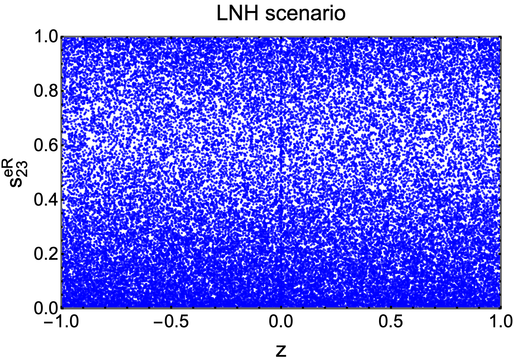
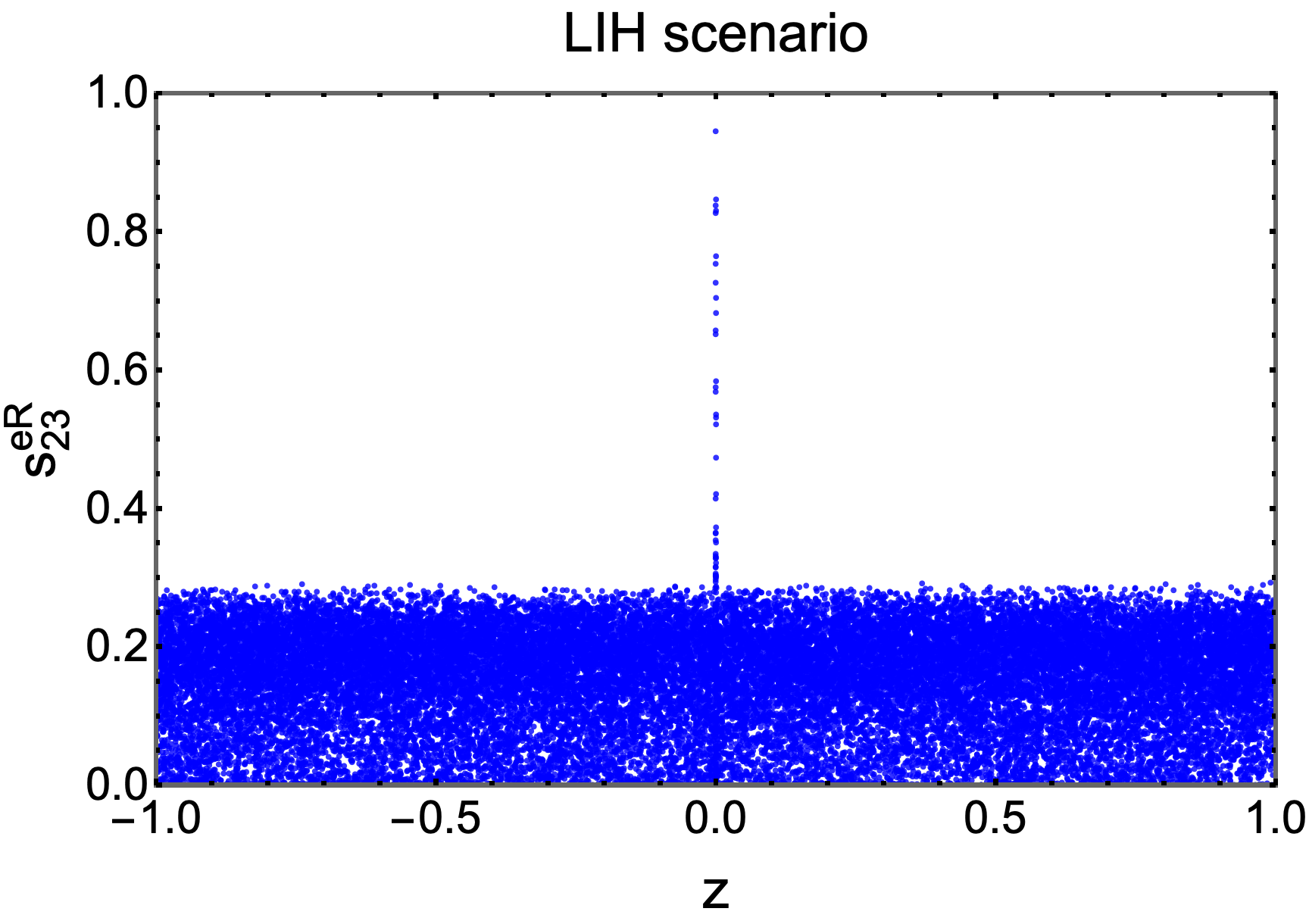
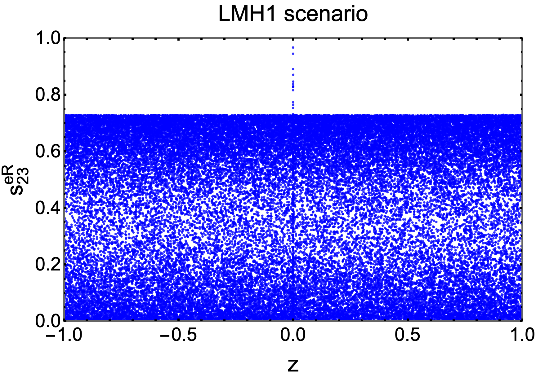
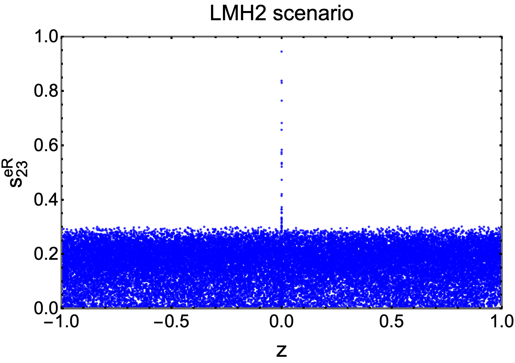
Figure 4: The correlations between mixing angle $s_{23}^{e_{R}}$ with charge parameter $z$ in four hierarchy scenarios of lepton mixing angles $\theta_{ij}^{e_{R}}$.

Furthermore, we obtain the correlation between the ratio $k=\Lambda_{1}/\Lambda_{2}$ and VEV $\Lambda_{2}$ within four hierarchy scenarios of lepton mixing angles $\theta_{ij}^{e_{R}}$, as respectively shown in four panels of Fig. 5. We see that the whole ranges of $k$ and $\Lambda_{2}$ in four panels generally satisfy the leptonic constraints, although these points distribute mainly with high $k$ and $\Lambda_{2}$ values, namely $k\gtrsim 7.4$ and $\Lambda_{2}\gtrsim 39$ TeV. Besides, the panels of LIH and LMH2 scenarios are almost similar. This result also occurred in Fig. 4. Hence, we comment that the LIH and LMH2 scenarios give the same results, while the LNH and LMH1 scenarios do not change considerably. Therefore, in the following, we consider the model under only the LNH and LIH scenarios that satisfy the constraints from the lepton flavor violation process.

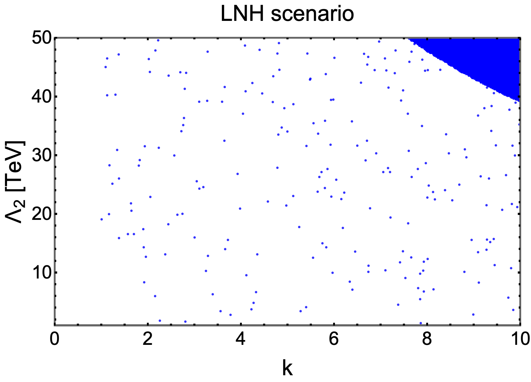
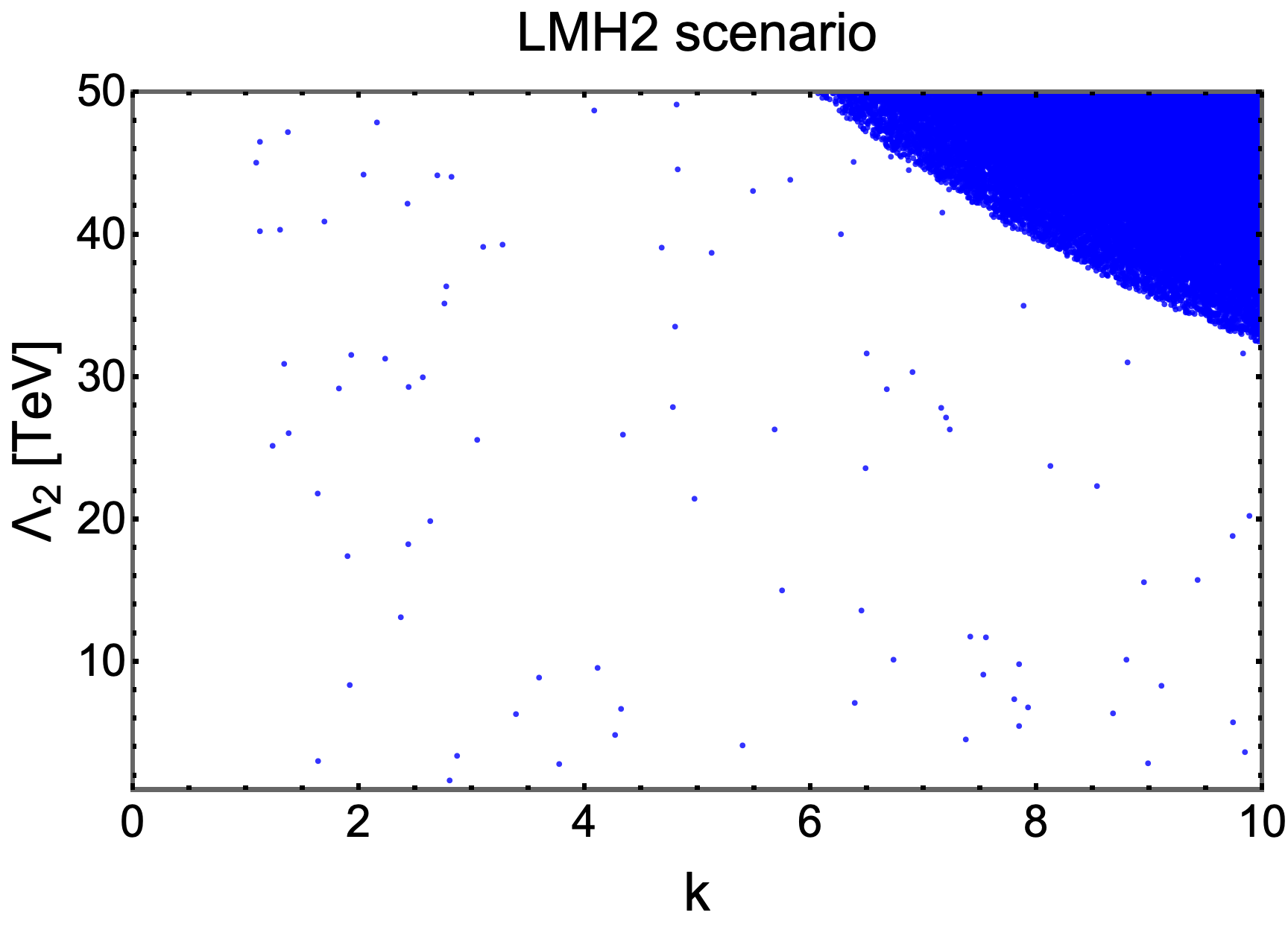
Figure 5: The correlations between the ratio $k=\Lambda_{1}/\Lambda_{2}$ with VEV $\Lambda_{2}$ for the four hierarchy scenarios of lepton mixing angles $\theta_{ij}^{e_{R}}$.

Now, we turn to the quark flavor phenomenologies. We randomly generate the free parameters $z,k$, $\Lambda_{2}$, and $\theta$ similarly in the studies of leptonic flavor phenomenologies. Besides, the parameters $s_{12}^{d_{R}}$ and $\delta^{d_{R}}$ are randomly extracted from ranges as

$$s_{12}^{d_{R}}\in[0,1],\hskip 14.22636pt\delta^{d_{R}}\in[-2\pi,2\pi],$$ (139)

whereas the lepton mixing angles $\theta_{ij}^{e_{R}}$ are chosen in the LNH and LIH scenarios.

In Fig. 6, we show the correlation points between the $\Delta m_{B_{s}}$ and $\Delta m_{B_{d}}$ in four hierarchy scenarios of quark mixing angles $\theta_{ij}^{d_{R}}$ determined by Eqs. (88)–(91), which satisfy the constraints of $\Delta m_{K}$, BR$(B_{s}\to\mu^{+}\mu^{-})$, and BR$(\bar{B}\to X_{s}\gamma)$ respectively expressed in Eqs. (128)–(130), and lepton mixing angle $\theta_{ij}^{e_{R}}$ is taken in the LNH scenario. The dot-dashed red and green lines are correspondingly the most current experimental limits of $\Delta m_{B_{s}}$ and $\Delta m_{B_{d}}$ [9]. It is important that the model with QNH scenario supplies points simultaneously fulfilling the constraints of both $\Delta m_{B_{s}}$ and $\Delta m_{B_{d}}$, whereas the QIH and QMH2 scenarios supply points adapt the constraint of only $\Delta m_{B_{d}}$. In addition, the QMH1 scenario provides points satisfying the constraint of either $\Delta m_{B_{s}}$ or $\Delta m_{B_{d}}$. A similar result is also shown in Fig. 7 plotted with the LIH scenario. These two figures imply that the model under QNH and LNH scenarios is preferred. Therefore, the following numerical studies will focus on these hierarchy scenarios.

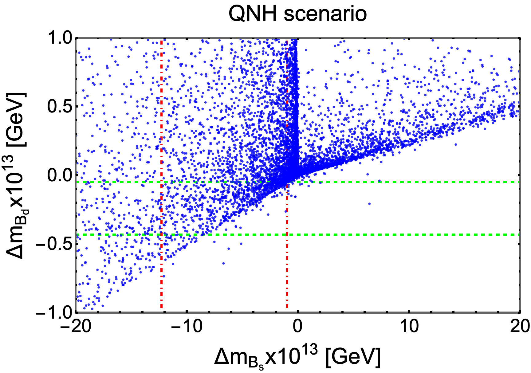
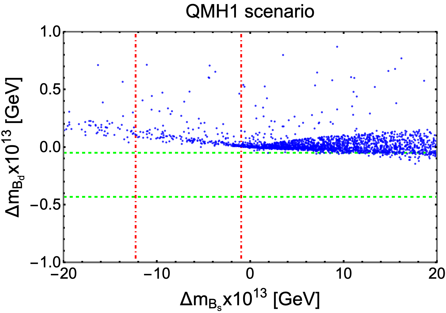
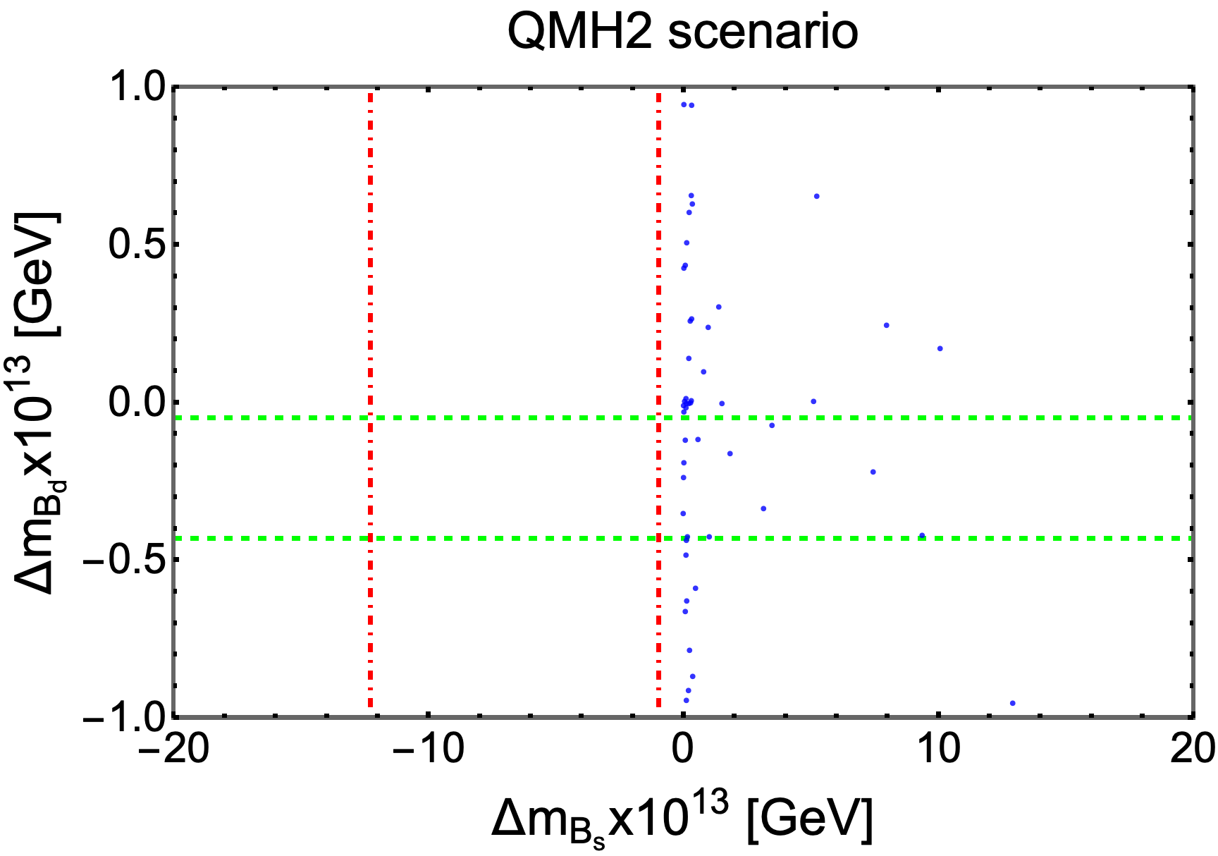
Figure 6: The correlations between predicted values of $\Delta m_{B_{s}}$ and $\Delta m_{B_{d}}$ for four hierarchy scenarios of quark mixing angles $\theta_{ij}^{d_{R}}$ with the LNH scenario of $\theta_{ij}^{e_{R}}$. The dot-dashed red and green lines present the experimental upper and lower limits of $\Delta m_{B_{s}}$ and $\Delta m_{B_{d}}$ [9].

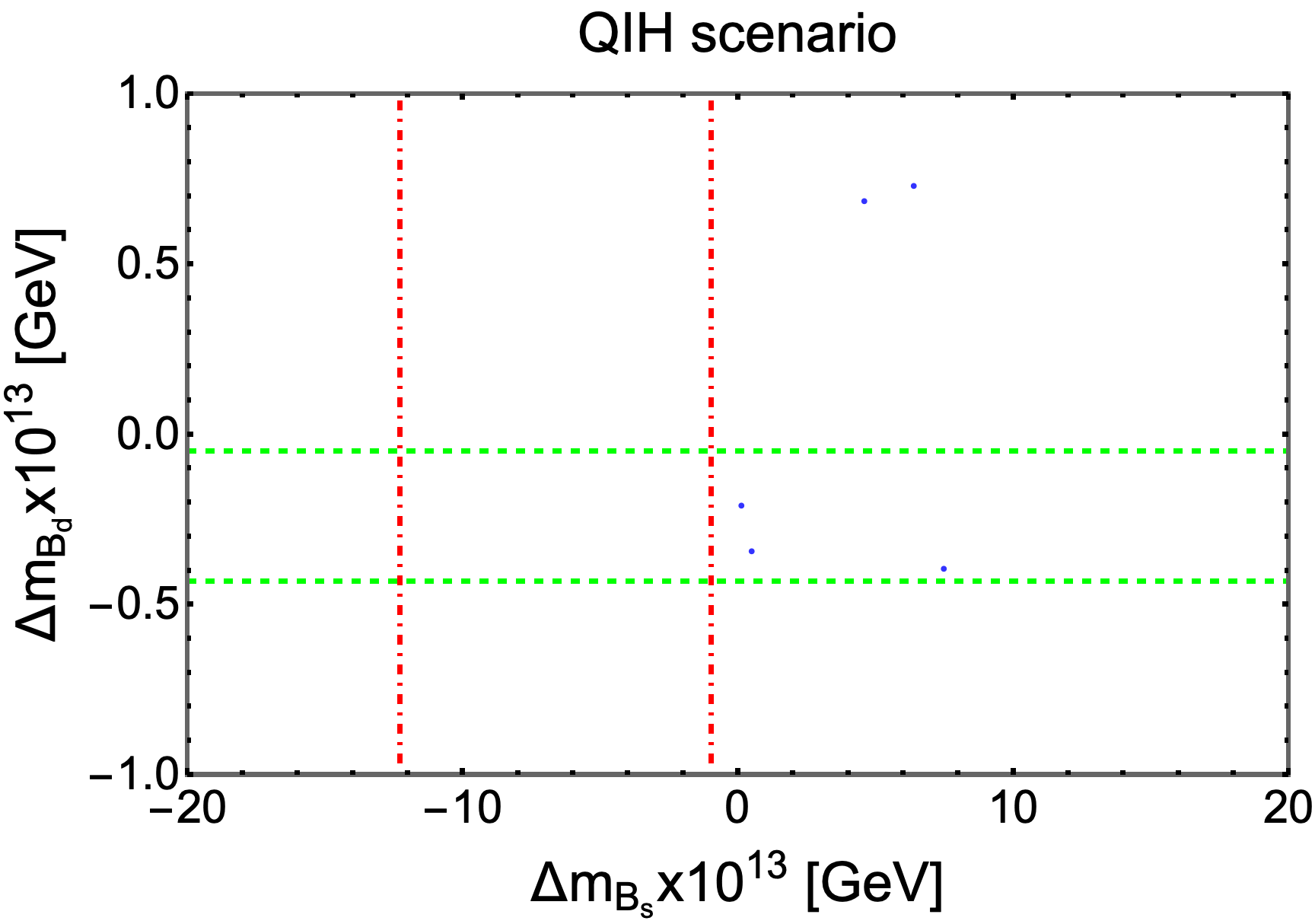
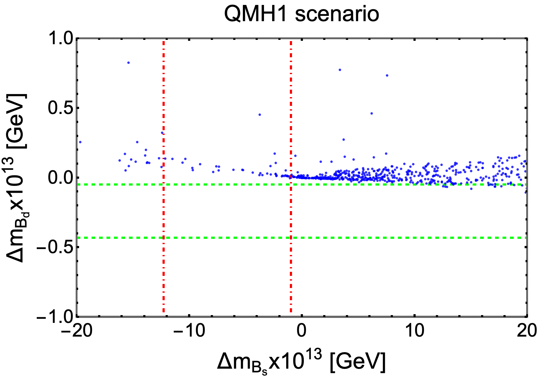
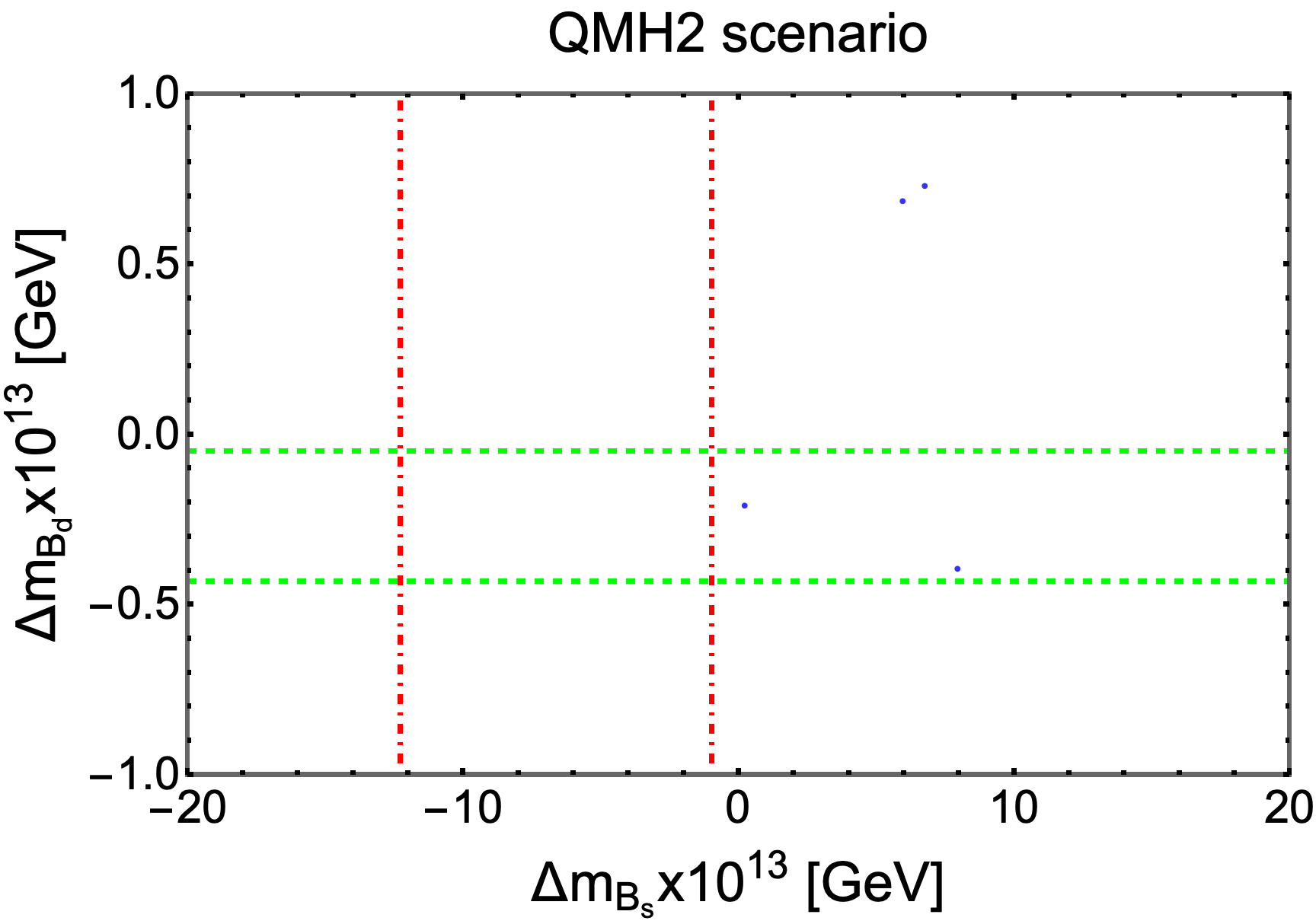
Figure 7: The correlations between predicted values of $\Delta m_{B_{s}}$ and $\Delta m_{B_{d}}$ in four hierarchy scenarios of quark mixing angles $\theta_{ij}^{d_{R}}$ with the LIH scenario of $\theta_{ij}^{e_{R}}$. The dot-dashed red and green lines present the experimental upper and lower limits of $\Delta m_{B_{s}}$ and $\Delta m_{B_{d}}$ [9].

Now, we focus particularly on four correlations, $s_{12}^{d_{R}}-z$, $s_{12}^{d_{R}}-s_{23}^{e_{R}}$, $s_{12}^{d_{R}}-\delta^{d_{R}}$, and $k-\Lambda_{2}$, which are respectively shown in four panels of Fig. 8. For the first panel, we see that the mixing angle $s_{12}^{d_{R}}$ is limited in a range $s_{12}^{d_{R}}\in[0.1,0.2]$ for $|z|\in[0.1,1]$. However, when $|z|$ decreases to less than 0.1, there are many points distributed in a wider range of $s_{12}^{d_{R}}$, i.e., $s_{12}^{d_{R}}\in[0.1,0.4]$. This can be interpreted by the following reason: when $|z|\sim 1$, the electroweak term proportional $v$ in $m_{Z^{\prime}}$ will be much smaller than one relevant to the new physics contribution and can be ignored. As a result, $m_{Z^{\prime}}$ now depends linearly on $z$, and then, several of the WCs are free of $z$ since it is canceled between numerator and denominator, such as the WCs in Eqs. (101)-(103) and (106)-(110). Therefore, the quark flavor observable is approximately independent of $z$. On the other hand, when $|z|$ is sufficiently small, the electroweak term significantly affects quark flavor processes. We would like to note that the upper limit of $s_{12}^{d_{R}}\sim 0.4$ is larger than the center value of $s_{12}^{\text{CKM}}=\lambda$ given in the Table 5. The second panel demonstrates that the mixing parameter $s_{12}^{d_{R}}$ of $V_{d_{R}}$ is independent of mixing parameter $s_{23}^{e_{R}}$ of $V_{e_{R}}$. The range of $s_{23}^{e_{R}}$ is not constrained tightly as the $s_{12}^{d_{R}}$ and whole range of $s_{23}^{e_{R}}$ satisfying the mentioned constraints. The correlation between $s_{12}^{d_{R}}$ with CP violation phase $\delta^{d_{R}}$ is displayed in the third panel. Here, the total range of $\delta^{d_{R}}$ fulfills the constraints from Eqs. (126) and (128)–(130). This also implies that the effect of $\delta^{d_{R}}$ on the quark flavor observables is negligible and can be ignored. The last panel focuses on the correlation between $k$ and $\Lambda_{2}$. It is easy to see that the behavior of $k$ and $\Lambda_{2}$ is inverse; if the value of $k$ increases then $\Lambda_{2}$ decreases. Additionally, when $k$ becomes much larger than $10$, $\Lambda_{2}$ tends to the regime of $\mathcal{O}(10^{2})$ GeV , which is inconsistent with the condition $\Lambda_{1,2}\gg v=246$ GeV. Therefore, to the new physics scale in the TeV scale, the relevant values of $k$ should be $k\leq 10$.

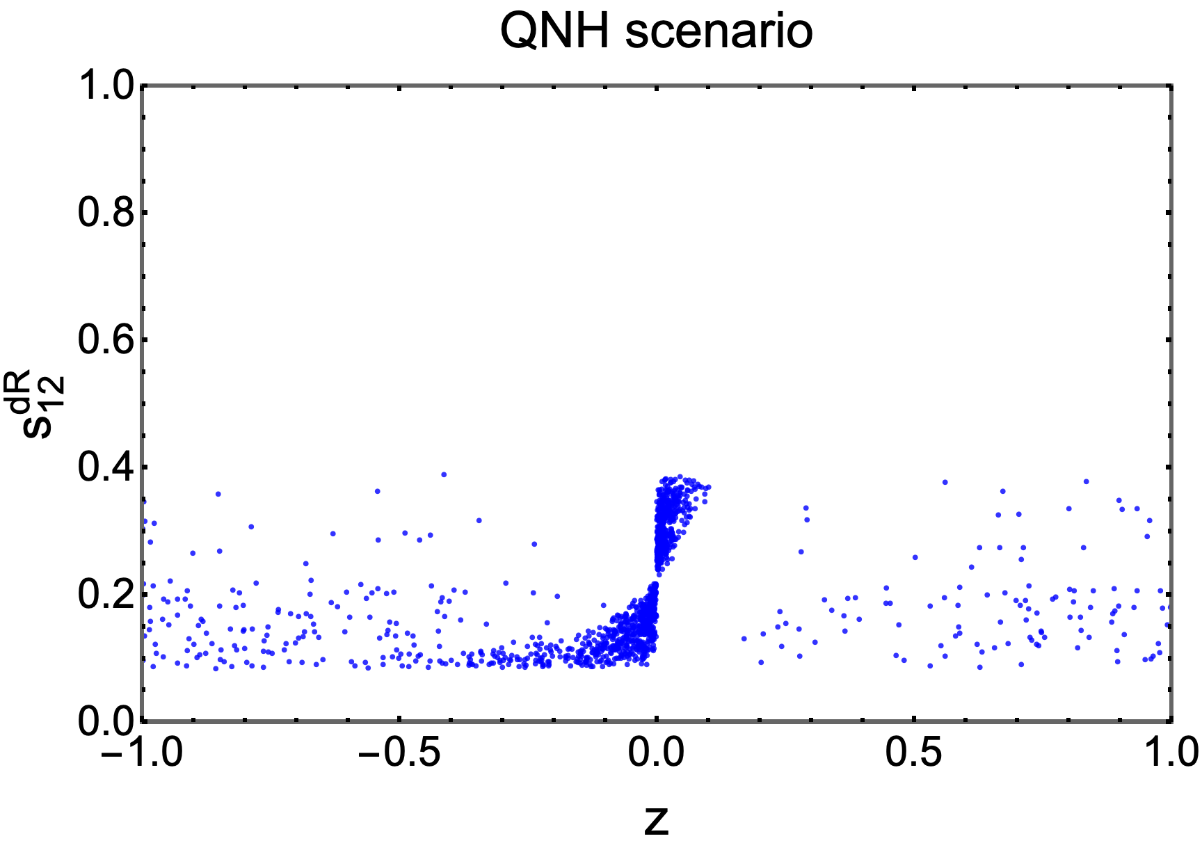
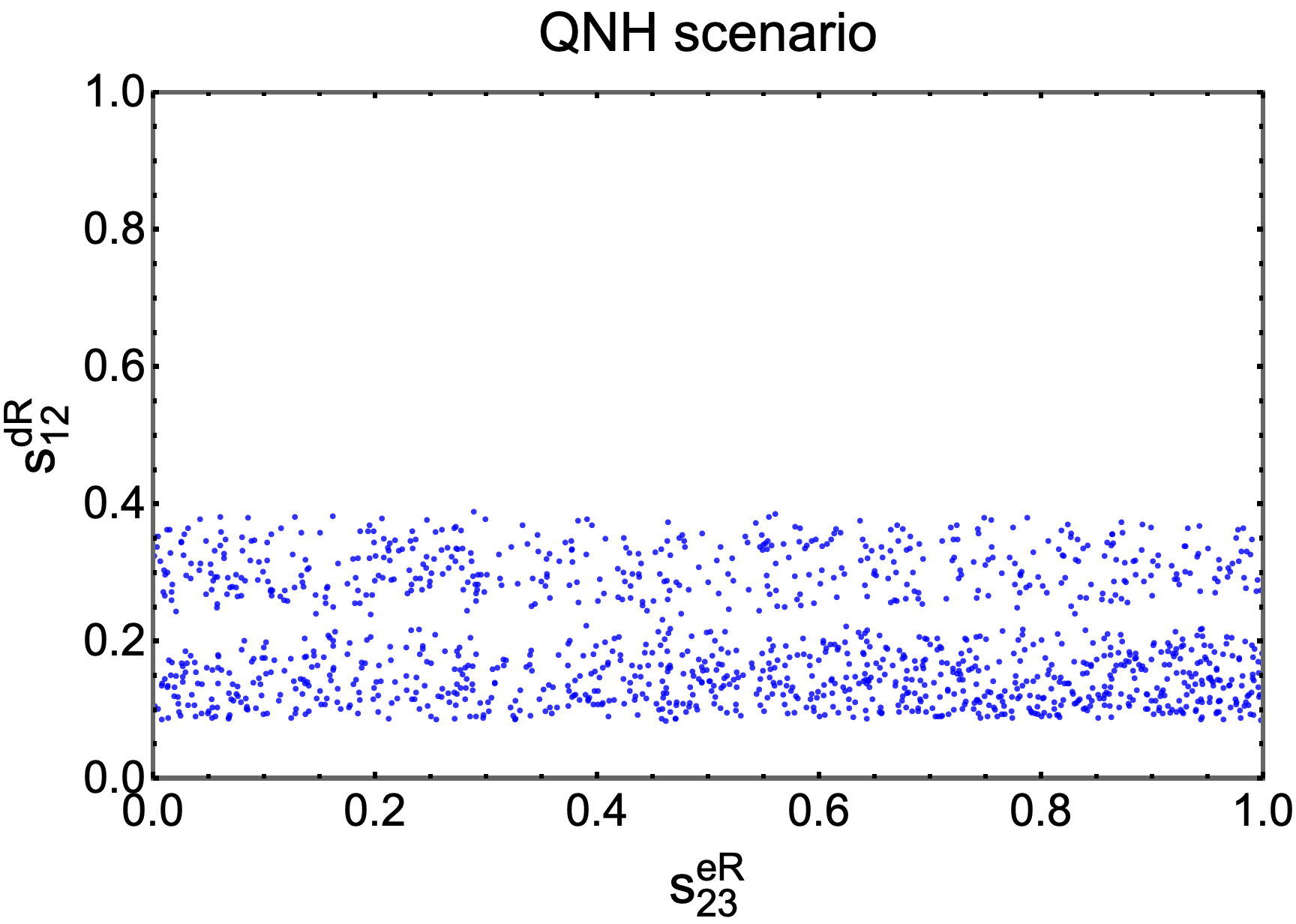
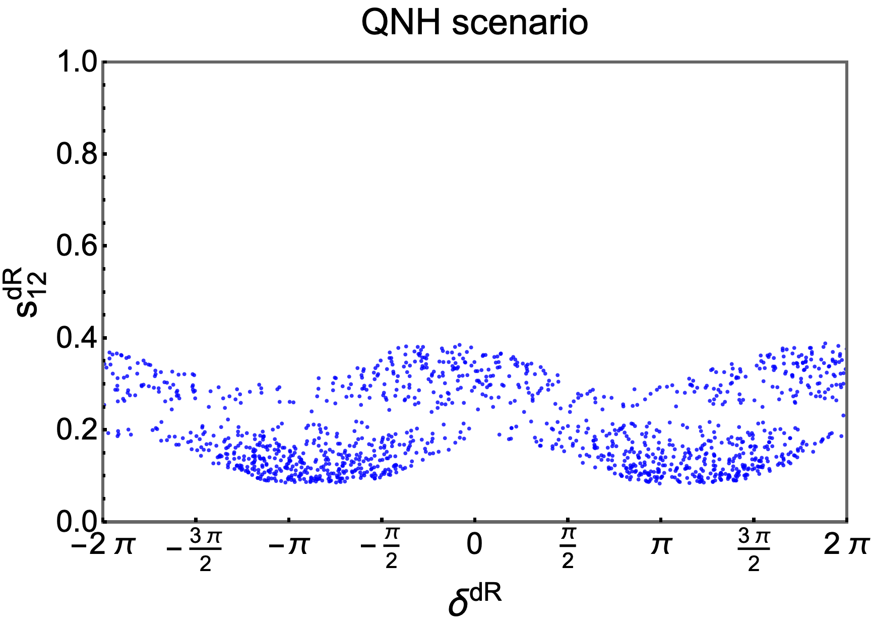
Figure 8: The correlation between parameter pairs, $s_{12}^{d_{R}}-z$, $s_{12}^{d_{R}}-s_{23}^{e_{R}}$, $s_{12}^{d_{R}}-\delta^{d_{R}}$, and $k-\Lambda_{2}$.

In Fig. 9, we show two correlations, $m_{Z^{\prime}}-z$ (left panel) and $m_{Z^{\prime}}-\theta$ (right panel). From here, we comment that the viable range of $z$ is $[-0.5,0.1]$, whereas the whole range of $\theta$ is available. However, if $\theta\in[5\pi/16,\pi/2)$ then $m_{Z^{\prime}}\gtrsim 6$ TeV. This is consistent with the collider bounds (discussed below). Comparing with Fig. 8, we obtain the viable ranges for several parameters as

$$s_{12}^{d_{R}}\in[0.1,0.22],\hskip 14.22636ptz\in[-0.5,0.1],\hskip 14.22636pt\theta\in[5\pi/16,\pi/2),\hskip 14.22636ptk\leq 10,\hskip 14.22636pts_{23}^{e_{R}}\in[0,1],$$ (140)

while the effect of $\delta^{d_{R}}$ is insignificantly and it can be chosen arbitrarily.

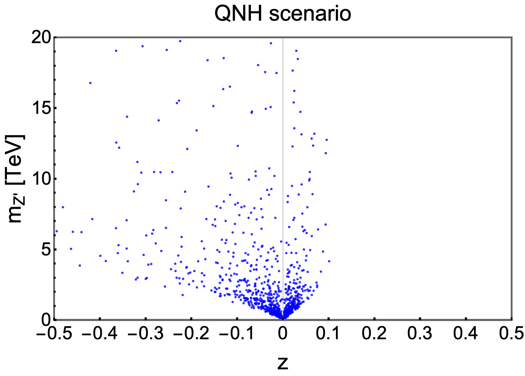
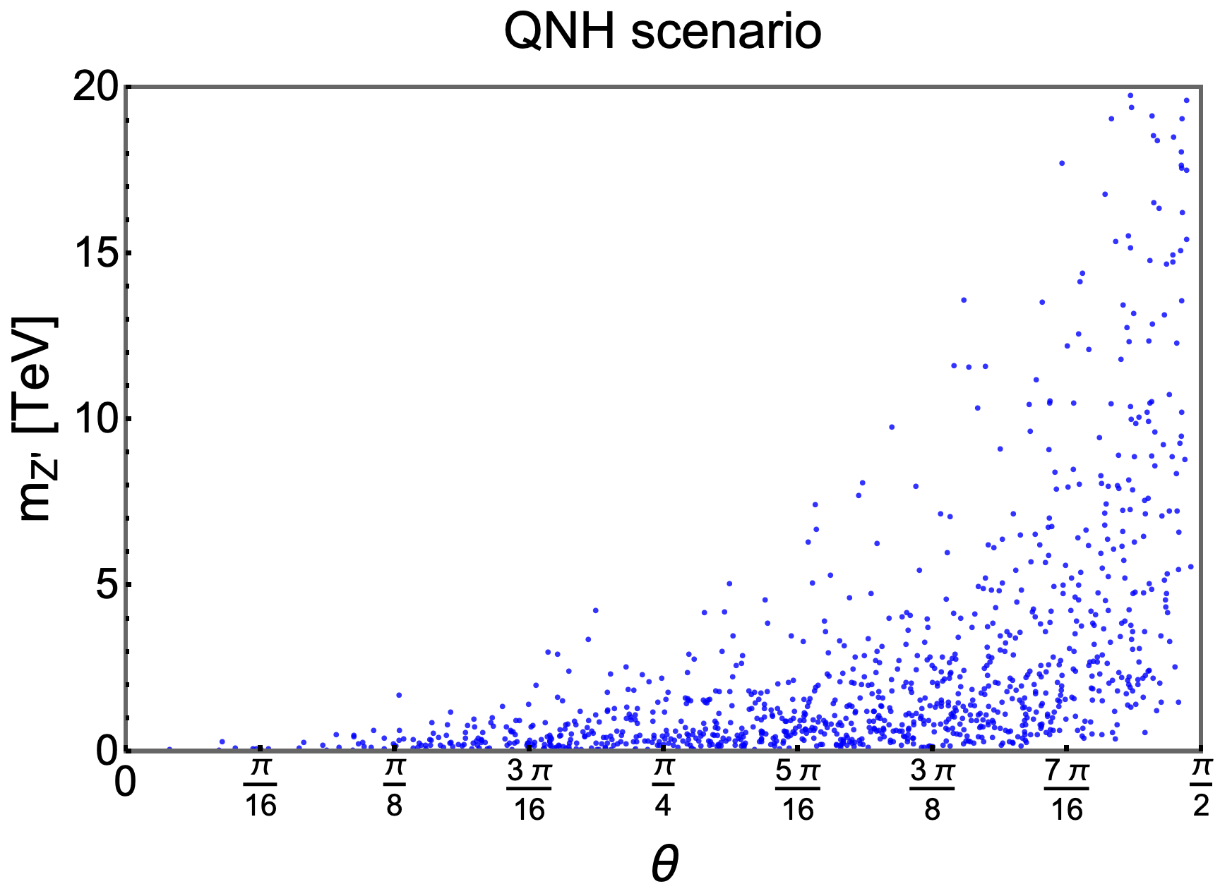
Figure 9: The correlation between the mass of new gauge boson $m_{Z^{\prime}}$ with the charge parameter $z$ (left panel), and with the mixing angle $\theta$ (right panel).

Last but not least, we consider the LFUV ratios $R_{K}$ and $R_{K^{*}}$; their results are shown in Fig. 10. The blue points are plotted in which parameters satisfy all constraints given in Eqs. (126) and (128)–(130). We realize that the figure shows points concurrently meeting the measured results of both $R_{K}$ and $R_{K^{*}}$ given in the last column in Table 7. Therefore, the model with the QNH hierarchy scenario can explain several of quark flavor observables, including the meson oscillations $\Delta m_{K,B_{s},B_{d}}$, BR$(\bar{B}\to X_{s}\gamma)$, BR$(B_{s}\to\mu^{+}\mu^{-})$, and $R_{K^{(*)}}$.

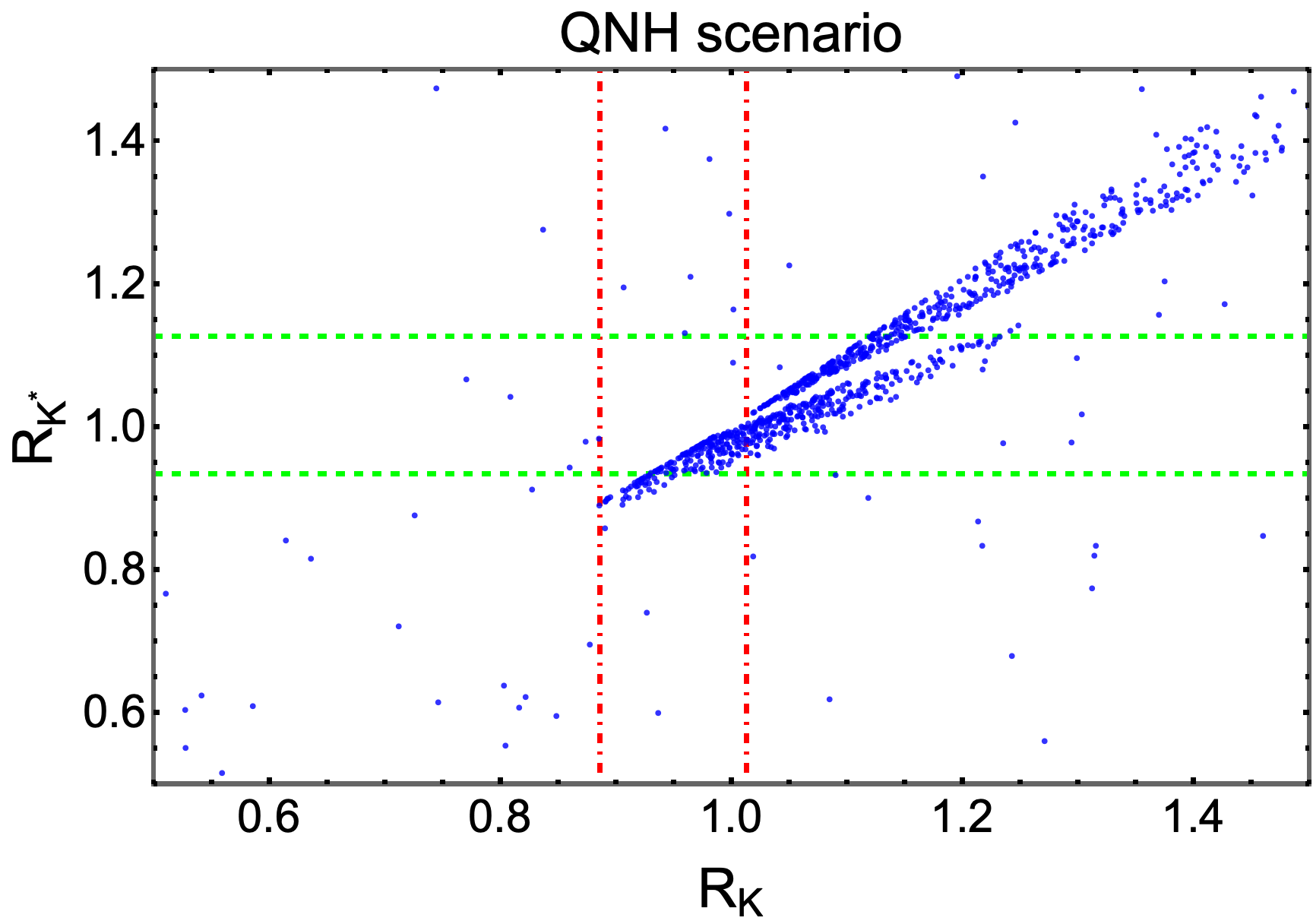
Figure 10: The correlation between the predicted $R_{K}$ and $R_{K^{*}}$. The dot-dashed red and green lines are correspondingly the current experimental limits of $R_{K}^{\text{exp}}$ and $R_{K^{*}}^{\text{exp}}$ [10].

VII Collider bounds

The $Z^{\prime}$ gauge boson in our model directly interacts with both ordinary quarks ($q$) and charged leptons ($l$), so it can be produced at the large electron-positron (LEP) experiments even the large hadron collider (LHC). In this section, we take the current negative search results reported by these experiments to impose a lower bound on the mass of $Z^{\prime}$ boson [58, 59, 60, 61, 62, 63].

VII.1 LEP

One of the processes searched at the LEP experiments is $e^{+}e^{-}\to f\bar{f}$, which generates a pair of ordinary charged leptons ($f=e,\mu,\tau$) through the exchange of $Z^{\prime}$ boson. This process can be described by the following effective Lagrangian,

$$\mathcal{L}_{\text{eff}}=\frac{1}{1+\delta_{ef}}\frac{g^{2}}{c^{2}_{W}m^{2}_{Z^{\prime}}}\sum_{i,j=L,R}C_{i}^{Z^{\prime}}(e)C_{j}^{Z^{\prime}}(f)(\bar{e}\gamma_{\mu}P_{i}e)(\bar{f}\gamma^{\mu}P_{j}f),$$ (141)

where $\delta_{ef}=1(0)$ for $f=e(\neq e)$, and the chiral gauge couplings are given by $C_{L,R}^{Z^{\prime}}(f)=\frac{1}{2}[g_{V}^{Z_{2}}(f)\pm g_{A}^{Z_{2}}(f)]$. LEP-II has probed all such effective contact interactions, and no significant evidence has been found for the existence of a $Z^{\prime}$ boson. LEP-II also provided the lower limits of the scale of the contact interactions, $\Lambda$, for all possible chiral structures and for various combinations of fermions [60]. Consequently, the mass of $Z^{\prime}$ boson is bounded by

$$m^{2}_{Z^{\prime}}\gtrsim\frac{g^{2}}{4\pi c^{2}_{W}}|C_{i}^{Z^{\prime}}(e)C_{j}^{Z^{\prime}}(f)|[\Lambda_{ij}^{\pm}(f)]^{2},$$ (142)

where $\Lambda^{+}$ for $C_{i}^{Z^{\prime}}(e)C_{j}^{Z^{\prime}}(f)>0$ and $\Lambda^{-}$ for $C_{i}^{Z^{\prime}}(e)C_{j}^{Z^{\prime}}(f)<0$.

The strongest constraint for our model comes from the $e^{+}e^{-}\to\mu^{+}\mu^{-},\tau^{+}\tau^{-}$ channel with $\Lambda^{+}_{VV}=24.6$ TeV. It results $m_{Z^{\prime}}\gtrsim 5.6$ TeV for $z\simeq-0.1$ and $\theta\simeq 3\pi/8$.

VII.2 LHC

At the LHC experiment, the $Z^{\prime}$ neutral gauge boson can be resonantly produced in the new physics processes $pp\to Z^{\prime}\to f\bar{f}$ for $f=q,l$. Additionally, the most significant decay channel of $Z^{\prime}$ is given by $Z^{\prime}\to l\bar{l}$ because of well-understood backgrounds [61, 63] and that it signifies a boson $Z^{\prime}$ having both couplings to lepton and quark like ours. The cross-section for the relevant process, in the narrow width approximation, takes the form [64]

$$\sigma(pp\to Z^{\prime}\to l\bar{l})\simeq\frac{1}{3}\sum_{q}\frac{dL_{q\bar{q}}}{dm_{Z^{\prime}}^{2}}\hat{\sigma}(q\bar{q}\to Z^{\prime})\text{BR}(Z^{\prime}\to l\bar{l}),$$ (143)

where the parton luminosities $\frac{dL_{q\bar{q}}}{dm_{Z^{\prime}}^{2}}$ can be found in Ref. [65], while the peak cross-section is given by

$$\hat{\sigma}(q\bar{q}\to Z^{\prime})\simeq\frac{\pi g^{2}}{12c_{W}^{2}}[(g_{V}^{Z_{2}}(q))^{2}+(g_{A}^{Z_{2}}(q))^{2}].$$ (144)

The branching ratio of $Z^{\prime}$ decaying into the lepton pairs is $\text{BR}(Z^{\prime}\to l\bar{l})=\Gamma(Z^{\prime}\to l\bar{l})/\Gamma_{Z^{\prime}}$, where the partial and total decay widths are respectively given by

$$\Gamma(Z^{\prime}\to l\bar{l}) \simeq \frac{g^{2}m_{Z^{\prime}}}{48\pi c_{W}^{2}}[(g_{V}^{Z_{2}}(l))^{2}+(g_{A}^{Z_{2}}(l))^{2}],$$ (145)

$$\Gamma_{Z^{\prime}} \simeq \frac{g^{2}m_{Z^{\prime}}}{48\pi c_{W}^{2}}\left\{\sum_{f}N_{C}(f)[(g_{V}^{Z_{2}}(f))^{2}+(g_{A}^{Z_{2}}(f))^{2}]+\frac{(C_{1L}^{Z_{2}})^{2}}{2}+(C_{2L}^{Z_{2}})^{2}\right\}$$ (146)

$$+\frac{g^{2}m_{Z^{\prime}}}{96\pi c_{W}^{2}}(C_{R}^{Z_{2}})^{2}\sum_{i=1}^{3}\left(1-\frac{4M_{i}^{2}}{m_{Z^{\prime}}^{2}}\right)^{3/2}\Theta\left(\frac{m_{Z^{\prime}}}{2}-M_{i}\right),$$

assuming that $Z^{\prime}$ is lighter than new Higgs bosons $\mathcal{H}_{1,2}$ and $\mathcal{A}$. Here, $f$ denotes the SM charged fermions, $N_{C}(f)$ is the color number of the fermion $f$, and $\Theta$ is the step function.

Setting center-of-mass energy of $\sqrt{s}=13$ TeV and assuming $M_{1,2,3}=m_{Z^{\prime}}/3$, in Fig. 11, we plot the cross section for the relevant processes as a function of the $Z^{\prime}$ boson mass, given that $z=-0.1$ and $\theta=3\pi/8$. Here, we also include the upper limits on the cross-section of these processes reported by ATLAS [61] and CMS [63] experiments. We obtain a lower bound on the $Z^{\prime}$ boson mass of $5.9$ TeV under the $ee$ channel, while the $\mu\mu~{}(\tau\tau)$ channel even implies a more strict constraint. Significantly, these signal strengths are separated, which can be used to approve or rule out the model under consideration.

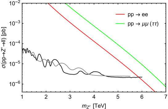
Figure 11: Dilepton production cross-section as a function of the new gauge boson mass $m_{Z^{\prime}}$ for $z=-0.1$ and $\theta=3\pi/8$. The black (gray) curve shows the upper bound on the cross-section obtained by the ATLAS 2019 results for $\Gamma/m=3\%$ [61] (the CMS 2019 results for $\Gamma/m=0.6\%$ [63]).

We would like to note that the dijet signals also can provide a lower bound for the $Z^{\prime}$ boson mass [62]. However, in the present model, the coupling strengths between $Z^{\prime}$ and the charged leptons are approximately equal to those of $Z^{\prime}$ with the quarks, while the current bound on dijet signals is less sensitive than the lepton one, so the lower bounds implied by the dijet search are quite smaller than those result from the dilepton. In other words, in the present model, the dijet bounds for the $Z^{\prime}$ boson mass are not significant.

VIII Conclusion

In this work, we have proposed a model that is based on the gauge symmetry $SU(3)_{C}\otimes SU(2)_{L}\otimes U(1)_{X}\otimes U(1)_{N}$. This model is general and flavor-dependent but constructed minimally. The new charges $X$ and $N$ of the light fermions differ from those of the remaining fermions but determine the hypercharge $Y$ as $Y=X+N$, which conforms to the observables. We have shown that our model can provide a possible solution to several puzzles of the SM, including the observed number of fermion generations, the neutrino mass generation mechanism, and the flavor anomalies in both the quark and lepton sectors. The new physics effects at the LEP and LHC experiments have also been examined.

With the relevant assumptions, the model leaves only six free parameters, including the charge parameter $z$, the new physics scale $\Lambda_{2}$, the ratio $k=\Lambda_{1}/\Lambda_{2}$, the mixing angles $\theta_{12}^{d_{R}}$, $\theta_{23}^{e_{R}}$ and $\theta$. We have identified the allowed parameter space of the model, which is consistent with the experimental constraints, namely, $\sin[\theta_{12}^{d_{R}}]\in[0.1,0.22],\hskip 14.22636ptz\in[-0.5,0.1],\hskip 14.22636pt\theta\in[5\pi/16,\pi/2),\hskip 14.22636ptk\in[1,10],\hskip 14.22636pt\sin[\theta_{23}^{e_{R}}]\in[0,1]$, and the new physics scale $\Lambda_{2}$ should generally be above several TeVs.

References

- [1] Particle Data Group collaboration, Review of Particle Physics, PTEP 2022 (2022) 083C01.
- [2] S. L. Glashow, Partial Symmetries of Weak Interactions, Nucl. Phys. 22 (1961) 579.
- [3] S. Weinberg, A Model of Leptons, Phys. Rev. Lett. 19 (1967) 1264.
- [4] A. Salam, Weak and Electromagnetic Interactions, Conf. Proc. C 680519 (1968) 367.
- [5] S. L. Glashow, J. Iliopoulos and L. Maiani, Weak Interactions with Lepton-Hadron Symmetry, Phys. Rev. D 2 (1970) 1285.
- [6] T. Kajita, Nobel Lecture: Discovery of atmospheric neutrino oscillations, Rev. Mod. Phys. 88 (2016) 030501.
- [7] A. B. McDonald, Nobel Lecture: The Sudbury Neutrino Observatory: Observation of flavor change for solar neutrinos, Rev. Mod. Phys. 88 (2016) 030502.
- [8] I. Esteban, M. C. Gonzalez-Garcia, M. Maltoni, T. Schwetz and A. Zhou, The fate of hints: updated global analysis of three-flavor neutrino oscillations, JHEP 09 (2020) 178 [2007.14792].
- [9] HFLAV collaboration, Averages of -hadron, -hadron, and -lepton properties as of 2021, 2206.07501.
- [10] LHCb collaboration, Measurement of the decay properties and search for the and decays, Phys. Rev. D 105 (2022) 012010 [2108.09283].
- [11] SINDRUM II collaboration, A Search for muon to electron conversion in muonic gold, Eur. Phys. J. C 47 (2006) 337.
- [12] BaBar collaboration, Searches for Lepton Flavor Violation in the Decays tau+- — e+- gamma and tau+- — mu+- gamma, Phys. Rev. Lett. 104 (2010) 021802 [0908.2381].
- [13] MEG collaboration, Search for the lepton flavour violating decay with the full dataset of the MEG experiment, Eur. Phys. J. C 76 (2016) 434 [1605.05081].
- [14] M. Singer, J. W. F. Valle and J. Schechter, Canonical Neutral Current Predictions From the Weak Electromagnetic Gauge Group SU(3) X (1), Phys. Rev. D 22 (1980) 738.
- [15] J. W. F. Valle and M. Singer, Lepton Number Violation With Quasi Dirac Neutrinos, Phys. Rev. D 28 (1983) 540.
- [16] F. Pisano and V. Pleitez, An SU(3) x U(1) model for electroweak interactions, Phys. Rev. D 46 (1992) 410 [hep-ph/9206242].
- [17] P. H. Frampton, Chiral dilepton model and the flavor question, Phys. Rev. Lett. 69 (1992) 2889.
- [18] R. Foot, H. N. Long and T. A. Tran, and gauge models with right-handed neutrinos, Phys. Rev. D 50 (1994) R34 [hep-ph/9402243].
- [19] P. V. Dong, H. N. Long, D. T. Nhung and D. V. Soa, SU(3)(C) x SU(3)(L) x U(1)(X) model with two Higgs triplets, Phys. Rev. D 73 (2006) 035004 [hep-ph/0601046].
- [20] P. V. Dong, H. N. Long and D. T. Nhung, Atomic parity violation in the economical 3-3-1 model, Phys. Lett. B 639 (2006) 527 [hep-ph/0604199].
- [21] P. V. Dong, D. T. Huong, N. T. Thuy and H. N. Long, Higgs phenomenology of supersymmetric economical 3-3-1 model, Nucl. Phys. B 795 (2008) 361 [0707.3712].
- [22] P. Van Dong and D. Van Loi, Scotoelectroweak theory, 2309.12091.
- [23] C. H. Nam, D. Van Loi, L. X. Thuy and P. Van Dong, Multicomponent dark matter in noncommutative gauge theory, JHEP 12 (2020) 029 [2006.00845].
- [24] P. Van Dong, T. N. Hung and D. Van Loi, Abelian charge inspired by family number, Eur. Phys. J. C 83 (2023) 199 [2212.13155].
- [25] D. Van Loi and P. Van Dong, Flavor-dependent U(1) extension inspired by lepton, baryon and color numbers, Eur. Phys. J. C 83 (2023) 1048 [2307.13493].
- [26] D. Van Loi, C. H. Nam and P. Van Dong, Phenomenology of a minimal extension of the standard model with a family-dependent gauge symmetry, Phys. Rev. D 108 (2023) 095018 [2305.04681].
- [27] J. C. Montero and V. Pleitez, Gauging U(1) symmetries and the number of right-handed neutrinos, Phys. Lett. B 675 (2009) 64 [0706.0473].
- [28] P. Van Dong, Interpreting dark matter solution for B-L gauge symmetry, Phys. Rev. D 108 (2023) 115022 [2305.19197].
- [29] P. V. Dong and H. N. Long, U(1)(Q) invariance and SU(3)(C) x SU(3)(L) x U(1)(X) models with beta arbitrary, Eur. Phys. J. C 42 (2005) 325 [hep-ph/0506022].
- [30] L.-L. Chau and W.-Y. Keung, Comments on the Parametrization of the Kobayashi-Maskawa Matrix, Phys. Rev. Lett. 53 (1984) 1802.
- [31] L. Wolfenstein, Parametrization of the Kobayashi-Maskawa Matrix, Phys. Rev. Lett. 51 (1983) 1945.
- [32] A. J. Buras, M. E. Lautenbacher and G. Ostermaier, Waiting for the top quark mass, K+ — pi+ neutrino anti-neutrino, B(s)0 - anti-B(s)0 mixing and CP asymmetries in B decays, Phys. Rev. D 50 (1994) 3433 [hep-ph/9403384].
- [33] CKMfitter Group collaboration, CP violation and the CKM matrix: Assessing the impact of the asymmetric factories, Eur. Phys. J. C 41 (2005) 1 [hep-ph/0406184].
- [34] Flavour Lattice Averaging Group (FLAG) collaboration, FLAG Review 2021, Eur. Phys. J. C 82 (2022) 869 [2111.09849].
- [35] UTfit collaboration, Fit results: summer 2018 at http://www.utfit.org/UTfit/ResultsSummer2018SM, .
- [36] M. Misiak, A. Rehman and M. Steinhauser, Towards at the NNLO in QCD without interpolation in , JHEP 06 (2020) 175 [2002.01548].
- [37] M. Misiak and M. Steinhauser, NNLO QCD corrections to the matrix elements using interpolation in , Nucl. Phys. B 764 (2007) 62 [hep-ph/0609241].
- [38] M. Czakon, U. Haisch and M. Misiak, Four-Loop Anomalous Dimensions for Radiative Flavour-Changing Decays, JHEP 03 (2007) 008 [hep-ph/0612329].
- [39] M. Beneke, C. Bobeth and R. Szafron, Enhanced electromagnetic correction to the rare -meson decay , Phys. Rev. Lett. 120 (2018) 011801 [1708.09152].
- [40] J. Charles et al., Current status of the Standard Model CKM fit and constraints on New Physics, Phys. Rev. D 91 (2015) 073007 [1501.05013].
- [41] G. Buchalla, A. J. Buras and M. E. Lautenbacher, Weak decays beyond leading logarithms, Rev. Mod. Phys. 68 (1996) 1125 [hep-ph/9512380].
- [42] F. Gabbiani, E. Gabrielli, A. Masiero and L. Silvestrini, A Complete analysis of FCNC and CP constraints in general SUSY extensions of the standard model, Nucl. Phys. B 477 (1996) 321 [hep-ph/9604387].
- [43] P. Langacker and M. Plumacher, Flavor changing effects in theories with a heavy boson with family nonuniversal couplings, Phys. Rev. D 62 (2000) 013006 [hep-ph/0001204].
- [44] A. Lenz and G. Tetlalmatzi-Xolocotzi, Model-independent bounds on new physics effects in non-leptonic tree-level decays of B-mesons, JHEP 07 (2020) 177 [1912.07621].
- [45] M. Beneke, C. Bobeth and R. Szafron, Power-enhanced leading-logarithmic QED corrections to , JHEP 10 (2019) 232 [1908.07011].
- [46] M. Bordone, G. Isidori and A. Pattori, On the Standard Model predictions for and , Eur. Phys. J. C 76 (2016) 440 [1605.07633].
- [47] R. Mohanta, Implications of the non-universal Z boson in FCNC mediated rare decays, Phys. Rev. D 71 (2005) 114013 [hep-ph/0503225].
- [48] K. De Bruyn, R. Fleischer, R. Knegjens, P. Koppenburg, M. Merk and N. Tuning, Branching Ratio Measurements of Decays, Phys. Rev. D 86 (2012) 014027 [1204.1735].
- [49] P. Gambino and M. Misiak, Quark mass effects in anti-B — X(s gamma), Nucl. Phys. B 611 (2001) 338 [hep-ph/0104034].
- [50] A. J. Buras, L. Merlo and E. Stamou, The Impact of Flavour Changing Neutral Gauge Bosons on , JHEP 08 (2011) 124 [1105.5146].
- [51] C. Cornella, D. A. Faroughy, J. Fuentes-Martin, G. Isidori and M. Neubert, Reading the footprints of the B-meson flavor anomalies, JHEP 08 (2021) 050 [2103.16558].
- [52] A. J. Buras and F. De Fazio, in 331 Models, JHEP 03 (2016) 010 [1512.02869].
- [53] A. Crivellin, M. Hoferichter and P. Schmidt-Wellenburg, Combined explanations of and implications for a large muon EDM, Phys. Rev. D 98 (2018) 113002 [1807.11484].
- [54] A. J. Buras, A. Crivellin, F. Kirk, C. A. Manzari and M. Montull, Global analysis of leptophilic Z’ bosons, JHEP 06 (2021) 068 [2104.07680].
- [55] Muon g-2 collaboration, Measurement of the Positive Muon Anomalous Magnetic Moment to 0.20 ppm, Phys. Rev. Lett. 131 (2023) 161802 [2308.06230].
- [56] ACME collaboration, Improved limit on the electric dipole moment of the electron, Nature 562 (2018) 355.
- [57] Muon (g-2) collaboration, An Improved Limit on the Muon Electric Dipole Moment, Phys. Rev. D 80 (2009) 052008 [0811.1207].
- [58] M. Carena, A. Daleo, B. A. Dobrescu and T. M. P. Tait, gauge bosons at the Tevatron, Phys. Rev. D 70 (2004) 093009 [hep-ph/0408098].
- [59] ALEPH, DELPHI, L3, OPAL, SLD, LEP Electroweak Working Group, SLD Electroweak Group, SLD Heavy Flavour Group collaboration, Precision electroweak measurements on the resonance, Phys. Rept. 427 (2006) 257 [hep-ex/0509008].
- [60] ALEPH, DELPHI, L3, OPAL, LEP Electroweak collaboration, Electroweak Measurements in Electron-Positron Collisions at W-Boson-Pair Energies at LEP, Phys. Rept. 532 (2013) 119 [1302.3415].
- [61] ATLAS collaboration, Search for high-mass dilepton resonances using 139 fb-1 of collision data collected at at , Phys. Lett. B 796 (2019) 68 [1903.06248].
- [62] ATLAS collaboration, Search for new resonances in mass distributions of jet pairs using 139 fb-1 of collisions at , JHEP 03 (2020) 145 [1910.08447].
- [63] CMS collaboration, Search for resonant and nonresonant new phenomena in high-mass dilepton final states at = 13 TeV, JHEP 07 (2021) 208 [2103.02708].
- [64] E. Accomando, A. Belyaev, L. Fedeli, S. F. King and C. Shepherd-Themistocleous, Z’ physics with early LHC data, Phys. Rev. D 83 (2011) 075012 [1010.6058].
- [65] A. D. Martin, W. J. Stirling, R. S. Thorne and G. Watt, Parton distributions for the LHC, Eur. Phys. J. C 63 (2009) 189 [0901.0002].