Comparison of two efficient numerical techniques based on Chelyshkov polynomial for solving stochastic Itô-Volterra integral equation

Abstract

In this study, two reliable approaches to solving the nonlinear stochastic Itô-Volterra integral equation are provided. These equations have been evaluated using the orthonormal Chelyshkov spectral collocation technique and the orthonormal Chelyshkov spectral Galerkin method. The techniques presented here transform this problem into a collection of nonlinear algebraic equations that have been numerically solved using the Newton method. Also, the convergence analysis has been studied for both approaches. Two illustrative examples have been provided to show the efficacy, plausibility, proficiency, and applicability of the current approaches.

Keywords: Stochastic Itô-Volterra integral equation; Itô integral; Itô approximation; Brownian motion; Chelyshkov polynomial; Galerkin method; Convergence analysis.

MSC: 60H20, 45D05, 60H05.

1 Introduction

Mathematical modelling of various scientific applications can be implemented using integral equations (IEs), such as integro-differential equations, Volterra integral equations [1], Fredholm integral equations [2], Volterra-Fredholm integral equations [3], etc. There has been a lot of interest in studying mathematical models utilising the Itô integral, particularly in science and engineering. Due to the fact that stochastic processes arise in several real problems, including turbulent flows [4], population dynamics [5], heat transfer problems [6], the Black-Scholes option pricing problem in mathematical finance [7], viscoelasticity problems [8], heat equation driven by an additive noise [9], and challenges in physics, chemistry, and biology [10]. The majority of practical problems are nonlinear. Since it is typical to solve nonlinear equations analytically, it is necessary to look into their numerical solutions. Some nonlinear processes can be determined by integral and integro-differential equations, partial integro differential equations (PDEs) [11], stochastic integral equations (SIEs) [12] and others. In the recent years, a variety of numerical techniques have been developed to solve linear and nonlinear integral and integro-differential equations such as Legendre spectral Galerkin method [13], Taylor expansion method [14], hybrid Legendre block pulse functions [15], triangular functions [16], Chebyshev wavelets [17], hat basis functions [18], Legendre wavelet operational method [19], Bernstein collocation method [20], shifted Jacobi operational matrix method [21], spectral collocation method [22] etc.

The main objective of this study is to find the numerical solution of the nonlinear stochastic Itô-Volterra integral equation (NSIVIE) as given by:

$$Z(\zeta)=Z_{0}+\delta_{1}\int_{0}^{\zeta}p(\eta,Z(\eta))d\eta+\delta_{2}\int_{0}^{\zeta}q(\eta,Z(\eta))dB(\eta),\quad\zeta,\eta\in[0,T],$$ (1.1)

where $\delta_{1}$ and $\delta_{2}$ are parameters and $Z_{0}$ is a random variable independent of $B(\zeta)$. $Z(\zeta)$, $p(\zeta,Z(\zeta))$ and $q(\zeta,Z(\zeta))$ for $\zeta\in[0,T]$ are stochastic processes defined on some probability space $(\Omega,\mathcal{F},\mathbb{P})$. $Z(\zeta)$ is an unknown function, that needs to be determined. This is referred to as the solution of eq. (1.1). Brownian motion is defined as $\{B(t),t\geq 0\}$ and $\int_{0}^{\zeta}q(\eta,Z(\eta))dB(\eta)$ is an Itô integral.

The following requirements are satisfied by the random functions $p(\zeta,Z(\zeta))$ and $q(\zeta,Z(\zeta))$ with probability 1, i.e.,

1. $p(\zeta,Z(\zeta))\in C([0,T]\times\mathbb{R},\mathbb{R})$ and $q(\zeta,Z(\zeta))\in C^{1}([0,T]\times\mathbb{R},\mathbb{R})$ are Borel-measurable.

2. $p(\zeta,Z(\zeta))$ and $q(\zeta,Z(\zeta))$ are uniformly continuous with respect to $\zeta$ and Lipschitz continuous with respect to $Z$.

In this article, the NSIVIE equation (1.1) is solved by using the orthonormal Chelyshkov spectral Galerkin (OCSG) method and the orthonormal Chelyshkov spectral collocation (OCSC) method. eq. (1.1) has been reduced to a nonlinear algebraic system of equations by using above-mentioned proposed methods. The resultant equations can be easily solved to get the desired approximate solution.

This manuscript is organized as follows:
Section 2 introduced fundamental concepts such as Brownian motion and the properties of Chelyshkov polynomials (CPs). A summary of the details of the spectral collocation technique and its convergence are presented in Section 3. In Section 4, the spectral Galerkin method is described. The NSIVIE problem is solved by using these two proposed methods. Section 5 demonstrates the efficacy and applicability of the suggested numerical approaches by considering two typical problems, and a brief summary is described in Section 6.

2 Preliminaries

This section discusses some basic stochastic calculus principles as well as the characteristics of Chelyshkov polynomial.

2.1 Stochastic calculus

Definition 1. ( Itô Integral [23]). Consider $\mathcal{V}=\mathcal{V}(U,V)$ be the class of functions $h(\alpha,\beta):[0,\infty)\times\Omega\rightarrow\mathbb{R}$ and $h\in\mathcal{V}(U,V)$. Thus, the definition of the Itô integral of $h$ is given by

$$\int_{U}^{V}h(\alpha,\beta)dB_{\alpha}(\beta)=\lim_{n\to\infty}\int_{U}^{V}\psi_{n}(\alpha,\beta)dB_{\alpha}(\beta)\quad(\lim in\,L^{2}(\mathbb{P})),$$ (2.1)

where $\{\psi_{n}\}$ is a sequence involving the elementary functions, satisfying the conditions given as:

$$E\left[\int_{U}^{V}(h(\alpha,\beta)-\psi_{n}(\alpha,\beta))^{2}d\alpha,\right]\rightarrow 0\,as\,n\rightarrow\infty.$$ (2.2)

Theorem 2.1.1 ( The Itô isometry [23]). Let $h\in\mathcal{V}(U,V)$, be elementary and bounded functions. Then

$$E\left[\left(\int_{U}^{V}h(\alpha,\beta)dB_{\alpha}(\beta)\right)^{2}\right]=E\left[\int_{U}^{V}h^{2}(\alpha,\beta)d\alpha\right].$$ (2.3)

Definition 2. ( Itô Approximation ). The following can be used to approximate the Itô integral $\int_{c}^{d}\psi(\zeta)dB(\zeta)$ for a measurable stochastic process $\psi$

$$\int_{c}^{d}\psi(\zeta)dB(\eta)\simeq\sum_{j=1}^{n}\psi(\zeta_{j-1})(B(\zeta_{j})-B(\zeta_{j-1})),$$ (2.4)

here, $n$ is an integer and $\zeta_{j}=c+\frac{(d-c)j}{n}$.

2.2 Chelyshkov polynomial and its properties

Chelyshkov recently introduced orthogonal polynomial sequences in the interval $[0,1]$ with the weight function 1. These polynomials are described as follows :

$$\phi_{i}(t)=\sum_{k=0}^{N-i}(-1)^{k}\binom{N-i}{k}\binom{N+k+i+1}{N-i}{t}^{k+i},\quad 0\leq i\leq N.$$ (2.5)

An $(N+1)$ set of the orthonormal Chelyshkov polynomials (OCPs) is defined over $[0,1]$ by

$$\phi^{*}_{i}(t)=\sqrt{2i+1}\sum_{k=0}^{N-i}(-1)^{k}\binom{N-i}{k}\binom{N+k+i+1}{N-i}{t}^{k+i},\quad 0\leq i\leq N.$$ (2.6)

The orthonormal property is given by

$$\int_{0}^{1}\phi^{*}_{i}(t)\phi^{*}_{j}(t)dt=\begin{cases}1&i=j\\ 0&i\mathrel{\vphantom{|}\mathchoice{\ooalign{$\displaystyle|$\cr$\displaystyle=$\cr}}{\ooalign{$\textstyle|$\cr$\textstyle=$\cr}}{\ooalign{$\scriptstyle|$\cr$\scriptstyle=$\cr}}{\ooalign{$\scriptscriptstyle|$\cr$\scriptscriptstyle=$\cr}}}j\end{cases}.$$ (2.7)

These polynomials are connected to the following set of Jacobi polynomials:

$$\phi_{i}(t)=(-1)^{N-i}{t}^{i}P^{0,2i+1}_{N-i}(2t-1),\quad i=0,1,2...,N.$$ (2.8)

3 Orthonormal Chelyshkov spectral collocation method

This section describes the orthonormal Chelyshkov spectral collocation method and its convergence analysis.

3.1 Methodology

The unknown function $Z(\zeta)$ in eq. (1.1) is approximated by Chelyshkov polynomial as follows

$$Z(\zeta)\simeq Z_{m}(\zeta):=\sum_{j=0}^{m}h_{j}\phi^{*}_{j}(\zeta),$$ (3.1)

where $h_{j},\{j=0,1,...,m\}$ are constants that need to be determined and $\phi^{*}_{j}(\zeta)$ is defined by eq. (2.6)

By substituting eq. (3.1) in eq. (1.1), the following is obtained

$$Z_{m}(\zeta)=Z_{0}+\delta_{1}\int_{0}^{\zeta}p(\eta,Z_{m}(\eta))d\eta+\delta_{2}\int_{0}^{\zeta}q(\eta,Z_{m}(\eta))dB(\eta),\quad\zeta,\eta\in[0,T],$$ (3.2)

whence

$$\sum_{j=0}^{m}h_{j}\phi^{*}_{j}(\zeta)=Z_{0}+\delta_{1}\int_{0}^{\zeta}p\left(\eta,\sum_{j=0}^{m}h_{j}\phi^{*}_{j}(\eta)\right)d\eta+\delta_{2}\int_{0}^{\zeta}q\left(\eta,\sum_{j=0}^{m}h_{j}\phi^{*}_{j}(\eta)\right)dB(\eta),\quad\zeta,\eta\in[0,T].$$ (3.3)

Using the $N$-point Gauss-Legendre quadrature algorithim, the first integral in eq. (3.3) is approximated as

$$\int_{0}^{\zeta}p\left(\eta,\sum_{j=0}^{m}h_{j}\phi^{*}_{j}(\eta)\right)d\eta\simeq\dfrac{\zeta}{2}\sum_{r=1}^{N}w_{r}p\left(\left(\frac{\zeta}{2}\tau_{r}+\frac{\zeta}{2}\right),\sum_{j=0}^{m}h_{j}\phi^{*}_{j}\left(\frac{\zeta}{2}\tau_{r}+\frac{\zeta}{2}\right)\right),$$ (3.4)

where nodes $\{\tau_{r}\}_{r=1}^{N}$ are the roots of $L_{N}$ on [-1, 1] and $w_{r},r=1,2,...,N$ are the corresponding weight functions.

Using the Itô approximation, the second integral in eq. (3.3) is approximated as follows

$$\int_{0}^{\zeta}q\left(\eta,\sum_{j=0}^{m}h_{j}\phi^{*}_{j}(\eta)\right)dB(\eta)\simeq\sum_{i=1}^{n}q\left(\left(\frac{(i-1)\zeta}{n}\right),\sum_{j=0}^{m}h_{j}\phi^{*}_{j}\left(\frac{(i-1)\zeta}{n}\right)\right)\left(B\left(\frac{i\zeta}{n}\right)-B\left(\frac{(i-1)\zeta}{n}\right)\right).$$ (3.5)

So, from eqs. (3.3)-(3.5), we get

$$\sum_{j=0}^{m}h_{j}\phi^{*}_{j}(\zeta)= Z_{0}+\delta_{1}\dfrac{\zeta}{2}\sum_{r=1}^{N}w_{r}p\left(\left(\frac{\zeta}{2}\tau_{r}+\frac{\zeta}{2}\right),\sum_{j=0}^{m}h_{j}\phi^{*}_{j}\left(\frac{\zeta}{2}\tau_{r}+\frac{\zeta}{2}\right)\right)$$

$$+\delta_{2}\sum_{i=1}^{n}q\left(\left(\frac{(i-1)\zeta}{n}\right),\sum_{j=0}^{m}h_{j}\phi^{*}_{j}\left(\frac{(i-1)\zeta}{n}\right)\right)\left(B\left(\frac{i\zeta}{n}\right)-B\left(\frac{(i-1)\zeta}{n}\right)\right).$$ (3.6)

Collocating eq. (3.6) by the Newton cotes collocation points given by $x_{k}=\dfrac{2k+1}{2(m+1)}T,\quad k=0,1,...,m$ generates a system of equations. This system contains $(m+1)$ nonlinear equations which can be solved for $(m+1)$ unknown coefficients ($h_{j}$) using suitable numerical technique. After that the final approximate solution is obtained by the equation $Z(\zeta)\simeq Z_{m}(\zeta):=\sum_{j=0}^{m}h_{j}\phi^{*}_{j}(\zeta)$.

3.2 Convergence analysis

Theorem 3.1.1 Suppose that $Z(\zeta)$ and $Z_{m}(\zeta)$ be the exact and approximate solutions of eq. (1.1) by the proposed OCSC method. Consider that the nonlinear terms in eq. (1.1) $p(\eta,Z(\eta))$ and $q(\eta,Z(\eta))$ are Lipschitz functions.

1. $||Z(\zeta)||\leq\infty,\forall\zeta\in[0,T],$
2. $|p(\eta,Z_{m}(\eta))-p(\eta,Z_{m}(\eta))|^{2}\leq M_{1}|Z(\eta)-Z_{m}(\eta)|^{2}$,
3. $|q(\eta,Z_{m}(\eta))-q(\eta,Z_{m}(\eta))|^{2}\leq M_{2}|Z(\eta)-Z_{m}(\eta)|^{2}$,
where $M_{1}$ and $M_{2}$ are positive constants.
Then,

$||Z(\zeta)-Z_{m}(\zeta)||^{2}\rightarrow 0,$

where

$||Z(\zeta)||^{2}=E[|Z(\zeta)|^{2}].$

Proof. The approximate solution of eq. (1.1) is given by

$$Z_{m}(\zeta)=Z_{0}+\delta_{1}\int_{0}^{\zeta}p(\eta,Z_{m}(\eta))d\eta+\delta_{2}\int_{0}^{\zeta}q(\eta,Z_{m}(\eta))dB(\eta),\quad\zeta,\eta\in[0,T].$$ (3.7)

Let $e_{m}(\zeta)=(Z(\zeta)-Z_{m}(\zeta))$ be an error function. Then

$$e_{m}(\zeta)=\delta_{1}\int_{0}^{\zeta}(p(\eta,Z(\eta))-p(\eta,Z_{m}(\eta)))d\eta+\delta_{2}\int_{0}^{\zeta}(q(\eta,Z(\eta))-q(\eta,Z_{m}(\eta)))dB(\eta)+E_{m}(\zeta).$$ (3.8)

Now, using the $N$-point Gauss-Legendre quadrature algorithim,

$$Z_{m}(\zeta)= Z_{0}+\delta_{1}\dfrac{\zeta}{2}\sum_{r=1}^{N}w_{r}p\left(\left(\frac{\zeta}{2}\tau_{r}+\frac{\zeta}{2}\right),\sum_{j=0}^{m}h_{j}\phi^{*}_{j}\left(\frac{\zeta}{2}\tau_{r}+\frac{\zeta}{2}\right)\right)$$

$$+\delta_{2}\sum_{i=1}^{n}q\left(\left(\frac{(i-1)\zeta}{n}\right),\sum_{j=0}^{m}h_{j}\phi^{*}_{j}\left(\frac{(i-1)\zeta}{n}\right)\right)\left(B\left(\frac{i\zeta}{n}\right)-B\left(\frac{(i-1)\zeta}{n}\right)\right).$$ (3.9)

Then

$$E_{m}(\zeta) =(\tilde{e}_{m}(\zeta))_{N,n}$$

$$=\delta_{1}\left[\int_{0}^{\zeta}p(\eta,Z(\eta))d\eta-\dfrac{\zeta}{2}\sum_{r=1}^{N}w_{r}p\left(\left(\frac{\zeta}{2}\tau_{r}+\frac{\zeta}{2}\right),\sum_{j=0}^{m}h_{j}\phi^{*}_{j}\left(\frac{\zeta}{2}\tau_{r}+\frac{\zeta}{2}\right)\right)\right]$$

$$+\delta_{2}\left[\int_{0}^{\zeta}q(\eta,Z(\eta))dB(\eta)-\sum_{i=1}^{n}q\left(\left(\frac{(i-1)\zeta}{n}\right),\sum_{j=0}^{m}h_{j}\phi^{*}_{j}\left(\frac{(i-1)\zeta}{n}\right)\right)\left(B\left(\frac{i\zeta}{n}\right)-B\left(\frac{(i-1)\zeta}{n}\right)\right)\right].$$ (3.10)

So, for large $N$ and $n$,

$$(\tilde{e}_{m}(\zeta))_{N,n}\rightarrow 0.$$ (3.11)

From eq. (3.8)

$$||e_{m}(\zeta)||\leq\delta_{1}||I_{1}(\zeta)||+\delta_{2}||I_{2}(\zeta)||+||E_{m}(\zeta)||,$$ (3.12)

where

$$I_{1}(\zeta)=\int_{0}^{\zeta}(p(\eta,Z(\eta))-p(\eta,Z_{m}(\eta)))d\eta,$$ (3.13)

and

$$I_{2}(\zeta)=\int_{0}^{\zeta}(q(\eta,Z(\eta))-q(\eta,Z_{m}(\eta)))dB(\eta).$$ (3.14)

For $I_{1}$, using the Lipschitz condition lead to

$$||I_{1}(\zeta)|| \leq\int_{0}^{\zeta}||p(\eta,Z(\eta))-p(\eta,Z_{m}(\eta))||d\eta$$

$$\leq M_{1}\int_{0}^{\zeta}||Z(\eta)-Z_{m}(\eta)||d\eta$$

$$=M_{1}\int_{0}^{\zeta}||e_{m}(\eta)||d\eta,$$

and for $I_{2}$, using the Itô isometry and Lipschitz condition, we get

$$||I_{2}(\zeta)|| =||\int_{0}^{\zeta}q(\eta,Z(\eta))-q(\eta,Z_{m}(\eta))dB(\eta)||$$

$$\leq\int_{0}^{\zeta}||q(\eta,Z(\eta))-q(\eta,Z_{m}(\eta))||d\eta$$

$$\leq M_{2}\int_{0}^{\zeta}||Z(\eta)-Z_{m}(\eta)||d\eta$$

$$=M_{2}\int_{0}^{\zeta}||e_{m}(\eta)||d\eta.$$

Now, substituting eqs. (3.15) and (3.16) into eq. (3.12), the following is obtained

$$||e_{m}(\zeta)|| \leq\delta_{1}M_{1}\int_{0}^{\zeta}||e_{m}(\eta)||d\eta+\delta_{2}M_{2}\int_{0}^{\zeta}||e_{m}(\eta)||d\eta+||E_{m}(\zeta)||$$

$$=(\delta_{1}M_{1}+\delta_{2}M_{2})\int_{0}^{\zeta}||e_{m}(\eta)||d\eta+||E_{m}(\zeta)||.$$

Thus, by using Grönwall inequality and $||E_{m}(\zeta)||\rightarrow 0$, we obtain

$||e_{m}(\zeta)||\rightarrow 0$ as $m\rightarrow\infty$,

So, $Z_{m}(\zeta)\rightarrow Z(\zeta)$ in $L^{2}$.

$\hskip 426.79134pt\blacksquare$

4 Orthonormal Chelyshkov spectral Galerkin method

The orthonormal Chelyshkov spectral Galerkin method and associated convergence analysis are discussed in this section.

4.1 Methodology

To solve NSIVIE, the OCSG method has been presented in this section. In order to do that, define an integral operator $P:C[0,T]\rightarrow C[0,T]$ by

$$(PZ)(\zeta):=\int_{0}^{\zeta}p(\eta,Z(\eta))d\eta,$$ (4.1)

and the Itô integral is given by

$$I_{\zeta}(Z):=\int_{0}^{\zeta}q(\eta,Z(\eta))dB(\eta).$$ (4.2)

Consequently, eq. (1.1) can be converted into the following form

$$Z(\zeta)=Z_{0}+\delta_{1}(PZ)(\zeta)+\delta_{2}I_{\zeta}(Z),\quad\zeta\in I:=[0,T],$$ (4.3)

and its weak form is to find $Z(\zeta)\in L^{2}([0,T])$ in such a way that

$$\langle Z(\zeta),X(\zeta)\rangle_{w}=\langle Z_{0},X(\zeta)\rangle_{w}+\delta_{1}\langle(PZ)(\zeta),X(\zeta)\rangle_{w}+\delta_{2}\langle I_{\zeta}(Z),X(\zeta)\rangle_{w},\text{ for any }X(\zeta)\in L^{2}([0,T]),$$ (4.4)

where $\langle.,.\rangle$ represents the inner product in the $L^{2}$ space and $w(\zeta)$ is a weight function.

For $m\in\mathbb{N}$, $\mathcal{T}_{m}$ be the set of all polynomials of degree at most $m$ in $[0,T]$.

The objective is to find: $Z_{m}(\zeta)\in\mathcal{T}_{m}$ such that

$$\langle Z_{m}(\zeta),X_{m}(\zeta)\rangle_{w}=\langle Z_{0},X_{m}(\zeta)\rangle_{w}+\delta_{1}\langle(PZ_{m})(\zeta),X_{m}(\zeta)\rangle_{w}+\delta_{2}\langle I_{\zeta}(Z_{m}),X_{m}(\zeta)\rangle_{w},\quad X_{m}(\zeta)\in\mathcal{T}_{m},$$ (4.5)

where $\mathcal{T}_{m}$ = span$\{\phi^{*}_{0}(\zeta),\phi^{*}_{1}(\zeta),...,\phi^{*}_{m}(\zeta)\}$.

Now, $Z_{m}(\zeta)=\sum_{j=0}^{m}h_{j}\phi^{*}_{j}(\zeta)$ and substituting it in eq. (4.5) and taking $X_{m}(\zeta)=\phi^{*}_{l}(\zeta)$, we obtain the following equation

$$\langle\sum_{j=0}^{m}h_{j}\phi^{*}_{j}(\zeta),\phi^{*}_{l}(\zeta)\rangle_{w}=\langle Z_{0},\phi^{*}_{l}(\zeta)\rangle_{w}+\delta_{1}\langle(P\left(\sum_{j=0}^{m}h_{j}\phi^{*}_{j}\right))(\zeta),\phi^{*}_{l}(\zeta)\rangle_{w}+\delta_{2}\langle I_{\zeta}(\left(\sum_{j=0}^{m}h_{j}\phi^{*}_{j}\right)),\phi^{*}_{l}(\zeta)\rangle_{w}.$$ (4.6)

Now, by using orthonormal property which is given in eq. (2.7), we obtain

$$\langle\sum_{j=0}^{m}h_{j}\phi^{*}_{j}(\zeta),\phi^{*}_{l}(\zeta)\rangle_{w}=h_{l}.$$ (4.7)

According to the inner product definition

$$\langle Z_{0},\phi^{*}_{l}(\zeta)\rangle_{w}=\int_{0}^{T}wZ_{0}\phi^{*}_{l}(\zeta)d\zeta,$$ (4.8)

$$\langle(P\left(\sum_{j=0}^{m}h_{j}\phi^{*}_{j}\right))(\zeta),\phi^{*}_{l}(\zeta)\rangle_{w}=\int_{0}^{T}w\left(\int_{0}^{\zeta}p\left(\eta,\sum_{j=0}^{m}h_{j}\phi^{*}_{j}(\eta)\right)d\eta\right)\phi^{*}_{l}(\zeta)d\zeta,$$ (4.9)

and

$$\langle I_{\zeta}(\left(\sum_{j=0}^{m}h_{j}\phi^{*}_{j}\right)),\phi^{*}_{l}(\zeta)\rangle_{w}=\int_{0}^{T}w\left(\int_{0}^{\zeta}q\left(\eta,\sum_{j=0}^{m}h_{j}\phi^{*}_{j}(\eta)\right)dB(\eta)\right)\phi^{*}_{l}(\zeta)d\zeta.$$ (4.10)

Using eq. (3.5) in eq. (4.10),

$$\langle I_{\zeta}(\left(\sum_{j=0}^{m}h_{j}\phi^{*}_{j}\right)),\phi^{*}_{l}(\zeta)\rangle_{w}\simeq\int_{0}^{T}w\phi^{*}_{l}(\zeta)\sum_{i=1}^{n} q\left(\left(\frac{(i-1)\zeta}{n}\right),\sum_{j=0}^{m}h_{j}\phi^{*}_{j}\left(\frac{(i-1)\zeta}{n}\right)\right)$$

$$\times\left(B\left(\frac{i\zeta}{n}\right)-B\left(\frac{(i-1)\zeta}{n}\right)\right)d\zeta.$$

Now, applying the $N$-point Gauss-Legendre quadrature algorithim, we obtain

$$\langle I_{\zeta}(\left(\sum_{j=0}^{m}h_{j}\phi^{*}_{j}\right)),\phi^{*}_{l}(\zeta)\rangle_{w}\simeq\dfrac{T}{2}\sum_{r=1}^{N} w\left(\frac{T}{2}\tau_{r}+\frac{T}{2}\right)w_{r}\phi^{*}_{l}\left(\frac{T}{2}\tau_{r}+\frac{T}{2}\right)$$

$$\times\sum_{i=1}^{n}q\left(\left(\frac{\left(\frac{T}{2}\tau_{r}+\frac{T}{2}\right)(i-1)}{n}\right),\sum_{j=0}^{m}h_{j}\phi^{*}_{j}\left(\frac{\left(\frac{T}{2}\tau_{r}+\frac{T}{2}\right)(i-1)}{n}\right)\right)$$

$$\times\left(B\left(\frac{\left(\frac{T}{2}\tau_{r}+\frac{T}{2}\right)i}{n}\right)-B\left(\frac{\left(\frac{T}{2}\tau_{r}+\frac{T}{2}\right)(i-1)}{n}\right)\right),$$

where nodes $\{\tau_{r}\}_{r=1}^{N}$ are the roots of $L_{N}$ on [-1, 1] and $w_{r},r=1,2,...,N$ are the corresponding weight functions.

Now, by using eqs. (4.7)-(4.9) and (4.12) in eq. (4.6), the following relation is obtained

$$h_{l}= \int_{0}^{T}wZ_{0}\phi^{*}_{l}(\zeta)d\zeta+\delta_{1}\int_{0}^{T}w\left(\int_{0}^{\zeta}p\left(\eta,\sum_{j=0}^{m}h_{j}\phi^{*}_{j}(\eta)\right)d\eta\right)\phi^{*}_{l}(\zeta)d\zeta$$

$$+\delta_{2}\dfrac{T}{2}\sum_{r=1}^{N}w\left(\frac{T}{2}\tau_{r}+\frac{T}{2}\right)w_{r}\phi^{*}_{l}\left(\frac{T}{2}\tau_{r}+\frac{T}{2}\right)$$

$$\times\sum_{i=1}^{n}q\left(\left(\frac{\left(\frac{T}{2}\tau_{r}+\frac{T}{2}\right)(i-1)}{n}\right),\sum_{j=0}^{m}h_{j}\phi^{*}_{j}\left(\frac{\left(\frac{T}{2}\tau_{r}+\frac{T}{2}\right)(i-1)}{n}\right)\right)$$

$$\times\left(B\left(\frac{\left(\frac{T}{2}\tau_{r}+\frac{T}{2}\right)i}{n}\right)-B\left(\frac{\left(\frac{T}{2}\tau_{r}+\frac{T}{2}\right)(i-1)}{n}\right)\right).$$ (4.13)

Thus, eq. (4.13) generates $(m+1)$ nonlinear equations with $(m+1)$ unknown coefficients ($h_{j},j=0,1,...,m$). Now, by solving these equations by suitable method, all the unknown coefficients are obtained. After that the final approximate solution by the OCSG method is obtained by the equation $Z(\zeta)\simeq Z_{m}(\zeta):=\sum_{j=0}^{m}h_{j}\phi^{*}_{j}(\zeta)$.

4.2 Convergence analysis

Let us define the Chelyshkov orthogonal projection operator

$$\Pi_{m}:L_{w}^{2}\rightarrow\mathcal{T}_{m},$$

which satisfies,

$\langle\Pi_{m}\delta Z,R_{m}\rangle_{w}=\delta\langle Z,R_{m}\rangle_{w}$ for any $Z\in L_{w}^{2},R_{m}\in\mathcal{T}_{m},$

where, $L_{w}^{2}(I)=\{R:R$ is a measurable and $||R||_{w}\leq\infty\}.$

Now, we define the Sobolev space $H^{l}(I)$ equipped with the norm and seminorm, which are defined as follows

$$||Y||_{H^{l}(I)}=\left(\sum_{k=0}^{l}||Y^{(k)}||^{2}_{L^{2}(I)}\right)^{\frac{1}{2}},$$

$$|Y|_{H^{l;m}(I)}=\left(\sum_{k=min(l,m+1)}^{l}||Y^{(k)}||^{2}_{L^{2}(I)}\right)^{\frac{1}{2}}.$$

Theorem 4.2.1 [24] Let $Z(\zeta)\in H^{\theta}(I),\theta\geq 1$ and $\Pi_{m}Z(\zeta)=\sum_{j=0}^{m}h_{j}\phi^{*}_{j}(\zeta)$ is the best approximation of $Z(\zeta)$, then

$$||Z-\Pi_{m}Z||_{L^{2}}\leq Cm^{-\theta}|Z|_{H^{\theta;m}(I)},$$

where

$$|Z|_{H^{l;m}(I)}=\left(\sum_{k=min(l,m+1)}^{l}\left(\dfrac{T}{2}\right)^{2l}||Z^{(k)}||^{2}_{L^{2}(I)}\right)^{\frac{1}{2}},$$

and $C$ depends on $\theta$.
According to the spectral method [25] and the concept of best approximation, which is unique, we obtain the desired results.

Theorem 4.2.2 Suppose that $Z(\zeta)\in H^{1;m}(I)$ be the exact solution and $Z_{m}(\zeta)$ be the OCSG method solution. Now, assume that

i)$|p(\zeta,Z_{1}(\zeta))-p(\eta,Z_{2}(\zeta))|^{2}\leq M_{1}|Z_{1}(\zeta)-Z_{2}(\zeta)|^{2},$
ii)$|q(\zeta,Z_{1}(\zeta))-q(\zeta,Z_{2}(\zeta))|^{2}\leq M_{2}|Z_{1}(\zeta)-Z_{2}(\zeta)|^{2}$,
iii) $5C^{2}m^{-2}\left(\dfrac{T}{2}\right)^{2}\left(|\delta_{1}|^{2}M_{1}^{2}+|\delta_{2}|^{2}M_{2}^{2}||\beta((\zeta)||^{2}\right)\leq 1$,

where $M_{1}$ and $M_{2}$ are positive constants.
Then $Z_{m}(\zeta)\rightarrow Z(\zeta)$ as $m\rightarrow\infty$ in $L^{2}$.

Proof: The approximate solution solution of eq. (1.1) is given by

$$Z_{m}(\zeta)=\Pi_{m}Z_{0}+\delta_{1}\Pi_{m}(PZ_{m})(\zeta)+\delta_{2}\Pi_{m}I_{\zeta}(Z_{m}),$$ (4.14)

and the exact solution is given by eq. (4.3). Then, the error is defined as

$$e(\zeta):=Z(\zeta)-Z_{m}(\zeta)=Z_{0}+\delta_{1}(PZ)(\zeta)+\delta_{2}I_{\zeta}(Z)-\Pi_{m}Z_{0}-\delta_{1}\Pi_{m}(PZ_{m})(\zeta)-\delta_{2}\Pi_{m}I_{\zeta}(Z_{m}).$$ (4.15)

Now,

$$\delta_{1}(PZ)(\zeta)-\delta_{1}\Pi_{m}(PZ_{m})(\zeta) =Z(\zeta)-\Pi_{m}Z(\zeta)-Z_{0}+\Pi_{m}Z_{0}-\delta_{2}I_{\zeta}(Z)+\Pi_{m}\delta_{2}I_{\zeta}(Z)$$

$$+\delta_{1}((PZ)(\zeta)-(PZ_{m})(\zeta))-\delta_{1}((PZ)(\zeta)-(PZ_{m})(\zeta))$$

$$+\Pi_{m}\delta_{1}((PZ)(\zeta)-(PZ_{m})(\zeta)).$$

By substituting eq. (4.16) into eq. (4.15)

$$e(\zeta) =Z(\zeta)-\Pi_{m}Z(\zeta)+\delta_{1}((PZ)(\zeta)-(PZ_{m})(\zeta))+\Pi_{m}\delta_{2}(I_{\zeta}(Z)-I_{\zeta}(Z_{m}))$$

$$-\left[\delta_{1}((PZ)(\zeta)-(PZ_{m})(\zeta))-\Pi_{m}\delta_{1}((PZ)(\zeta)-(PZ_{m})(\zeta))\right],$$

which can be written as

$$e(\zeta) =Z(\zeta)-\Pi_{m}Z(\zeta)+\delta_{1}((PZ)(\zeta)-(PZ_{m})(\zeta))+\delta_{2}(I_{\zeta}(Z)-I_{\zeta}(Z_{m}))$$

$$-\left[\delta_{1}((PZ)(\zeta)-(PZ_{m})(\zeta))-\Pi_{m}\delta_{1}((PZ)(\zeta)-(PZ_{m})(\zeta))\right]$$

$$-\left[\delta_{2}(I_{\zeta}(Z)-I_{\zeta}(Z_{m}))-\Pi_{m}\delta_{2}(I_{\zeta}(Z)-I_{\zeta}(Z_{m}))\right].$$

Now, by using inequality $||\sum_{k=1}^{M}y_{k}||^{2}\leq M\sum_{k=1}^{M}||y_{k}||^{2}$, we obtain

$$||e(\zeta)||^{2} \leq 5[||Z(\zeta)-\Pi_{m}Z(\zeta)||^{2}+||\delta_{1}((PZ)(\zeta)-(PZ_{m})(\zeta))||^{2}+||\delta_{2}(I_{\zeta}(Z)-I_{\zeta}(Z_{m}))||^{2}$$

$$+\||\delta_{1}((PZ)(\zeta)-(PZ_{m})(\zeta))-\Pi_{m}\delta_{1}((PZ)(\zeta)-(PZ_{m})(\zeta))||^{2}$$

$$+||\delta_{2}(I_{\zeta}(Z)-I_{\zeta}(Z_{m}))-\Pi_{m}\delta_{2}(I_{\zeta}(Z)-I_{\zeta}(Z_{m}))||^{2}].$$

Now, for $\theta=1$ applying Theorem 4.2.1

$$||Z(\zeta)-\Pi_{m}Z(\zeta)||^{2}\leq C^{2}m^{-2}|Z(\zeta)|^{2}_{H^{1;m}(I)}.$$ (4.20)

By using Lipschitz condition and Cauchy-Schwarz inequality, it follows that

$$||\delta_{1}((PZ)(\zeta)-(PZ_{m})(\zeta))||^{2} =E\left[\left|\delta_{1}\int_{0}^{\zeta}(p(\eta,Z(\eta))-p(\eta,Z_{m}(\eta)))d\eta\right|^{2}\right]$$

$$\leq|\delta_{1}|^{2}M_{1}^{2}\int_{0}^{\zeta}||e(\eta)||^{2}d\eta.$$

Now, by applying Itô isometry property and Lipschitz condition, we get

$$||\delta_{2}(I_{\zeta}(Z)-I_{\zeta}(Z_{m}))||^{2} =E\left[\left|\delta_{2}\int_{0}^{\zeta}(q(\eta,Z(\eta))-q(\eta,Z_{m}(\eta)))dB(\eta)\right|^{2}\right]$$

$$\leq|\delta_{2}|^{2}M_{1}^{2}\int_{0}^{\zeta}||e(\eta)||^{2}d\eta.$$

By using Theorem 4.2.1

$$||\delta_{1}((PZ)(\zeta)-(PZ_{m})(\zeta))-\Pi_{m}\delta_{1}((PZ)(\zeta)-(PZ_{m})(\zeta))||^{2}\leq C^{2}m^{-2}|\delta_{1}((PZ)(\zeta)-(PZ_{m})(\zeta))|^{2}_{H^{1;m}(I)}$$ (4.23)

Now,

$$|\delta_{1}((PZ)(\zeta)-(PZ_{m})(\zeta))|^{2}_{H^{1;m}(0,1)} =|\delta_{1}|^{2}\left(\dfrac{T}{2}\right)^{2}\left|\left|\frac{d}{d\zeta}\int_{0}^{\zeta}(p(\eta,Z(\eta))-p(\eta,Z_{m}(\eta)))d\eta\right|\right|^{2}$$

$$=|\delta_{1}|^{2}\left(\dfrac{T}{2}\right)^{2}||p(\zeta,Z(\zeta))-p(\zeta,Z_{m}(\zeta))||^{2}$$

$$=|\delta_{1}|^{2}\left(\dfrac{T}{2}\right)^{2}E|p(\zeta,Z(\zeta))-p(\zeta,Z_{m}(\zeta))|^{2}$$

$$\leq|\delta_{1}|^{2}\left(\dfrac{T}{2}\right)^{2}M_{1}^{2}||e(\zeta)||^{2}.$$

By substituting eq. (4.24) into eq. (4.23)

$$||\delta_{1}((PZ)(\zeta)-(PZ_{m})(\zeta))-\Pi_{m}\delta_{1}((PZ)(\zeta)-(PZ_{m})(\zeta))||^{2}\leq C^{2}m^{-2}|\delta_{1}|^{2}\left(\dfrac{T}{2}\right)^{2}|M_{1}^{2}||e(\zeta)||^{2}.$$ (4.25)

Again,

$$||\delta_{2}(I_{\zeta}(Z)-I_{\zeta}(Z_{m}))-\Pi_{m}\delta_{2}(I_{\zeta}(Z)-I_{\zeta}(Z_{m}))||^{2}\leq C^{2}m^{-2}|\delta_{2}(I_{\zeta}(Z)-I_{\zeta}(Z_{m}))|^{2}_{H^{1;m}(I)}$$ (4.26)

Now, by using stochastic Leibniz rule

$$|\delta_{2}(I_{\zeta}(Z)-I_{\zeta}(Z_{m}))|^{2}_{H^{1;m}(0,1)} =|\delta_{2}|^{2}\left(\dfrac{T}{2}\right)^{2}\left|\left|\frac{d}{d\zeta}\int_{0}^{\zeta}(q(\eta,Z(\eta))-q(\eta,Z_{m}(\eta)))dB\eta\right|\right|^{2}$$

$$=|\delta_{2}|^{2}\left(\dfrac{T}{2}\right)^{2}\left|\left|q(\zeta,Z(\zeta))-q(\zeta,Z_{m}(\zeta))\frac{dB(\zeta)}{d\zeta}\right|\right|^{2}$$

$$\leq|\delta_{2}|^{2}\left(\dfrac{T}{2}\right)^{2}M_{2}^{2}||e(\zeta)||^{2}||\beta(\zeta)||^{2},$$

where $\beta(\zeta)=\frac{dB(\zeta)}{d\zeta}$.

By substituting eq. (4.27) into eq. (4.26)

$$||\delta_{2}(I_{\zeta}(Z)-I_{\zeta}(Z_{m}))-\Pi_{m}\delta_{2}(I_{\zeta}(Z)-I_{\zeta}(Z_{m}))||^{2}\leq C^{2}m^{-2}|\delta_{2}|^{2}\left(\dfrac{T}{2}\right)^{2}M_{2}^{2}||e(\zeta)||^{2}||\beta(\zeta)||^{2}.$$ (4.28)

Now, all the results from eqs. (4.19), (4.20), (4.21), (4.22), (4.25) and (4.28), the following inequality has been obtained.

$$||e(\zeta)||^{2}\leq\alpha(\zeta)+L_{1}\int_{0}^{\zeta}||e(\eta)||^{2}d\eta,$$ (4.29)

where,

$$\alpha(\zeta)=\dfrac{5C^{2}m^{-2}|Z(\zeta)|^{2}_{H^{1;m}(I)}}{1-5C^{2}m^{-2}\left(\dfrac{T}{2}\right)^{2}\left(|\delta_{1}|^{2}M_{1}^{2}+|\delta_{2}|^{2}M_{2}^{2}||\beta((\zeta)||^{2}\right)},$$

$$L_{1}=\dfrac{5(|\delta_{1}|^{2}M_{1}^{2}+|\delta_{2}|^{2}M_{2}^{2})}{1-5C^{2}m^{-2}\left(\dfrac{T}{2}\right)^{2}\left(|\delta_{1}|^{2}M_{1}^{2}+|\delta_{2}|^{2}M_{2}^{2}||\beta((\zeta)||^{2}\right)}.$$

The Grönwall inequality for eq. (4.29) follows

$$||e(\zeta)||^{2}\leq\alpha(\zeta)\left(1+L_{1}\int_{0}^{\zeta}e^{L_{1}(\zeta-\eta)}d\eta\right).$$ (4.30)

By increasing $m$, it implies

$||e(\zeta)||^{2}\rightarrow 0$ as $m\rightarrow\infty.$

So,

$Z_{m}(\zeta)\rightarrow Z(\zeta)$ in $L^{2}$.

$\hskip 455.24408pt\blacksquare$

5 Illustrative examples

The numerical techniques provided in the previous section is used to solve the two problems presented in this section.

Problem 1. Consider the following nonlinear SIVIE :

$$Z(\zeta)=Z_{0}+\int_{0}^{\zeta}(\alpha Z(\eta)+\beta Z^{2}(\eta))d\eta+\gamma\int_{0}^{\zeta}Z(\eta)dB(\eta),\quad\zeta,\eta\in[0,1],$$ (5.1)

with the exact solution

$$Z(\zeta)=\dfrac{exp\left((\alpha-\frac{\gamma^{2}}{2})\zeta+\gamma B(\zeta)\right)}{\frac{1}{Z_{0}}-\beta\int_{0}^{\zeta}exp\left((\alpha-\frac{\gamma^{2}}{2})\eta+\gamma B(\eta)\right)d\eta},$$

where $\alpha,\beta,\gamma$ and $Z_{0}$ are constant and $Z(\zeta)$ is an unknown stochastic process.
For $\alpha=\frac{1}{8},\beta=\frac{1}{32},\gamma=\frac{1}{20}$ and $Z_{0}=\frac{1}{10}$, eq. (5.1) has been solved by using the two proposed approaches. For $m=4,6,8$ the problem is solved here. For OCSC method newton cotes nodes has been chosen as a collocation points. Tables 1-3 and tables 4-6 provide the exact, numerical solutions and absolute error by using OCSC method and OCSG method respectively. Table 7 provide the comparison between numerical solutions and absolute error by two presented OCSC and OCSG methods for $m=5$. Tables 8-9 represent mean ($\overline{Z}$), standard error ($S_{E}$), and 95 % mean confidence interval for absolute error in $10$ trials. Figures 1-3 represent the plot of exact solutions, numerical solutions and corresponding abosulute error behavior for different values of $m$ by two presented OCSC and OCSG methods.

Table 1: The OCSC solution for $m=4$ (Problem 1).

$\zeta$	Exact solution	OCSC method solution	Absolute error
0.1	0.100862	0.100894	3.23964 $\times 10^{-5}$
0.2	0.101036	0.106896	0.00585995
0.3	0.107904	0.107356	5.47881 $\times 10^{-4}$
0.4	0.107923	0.106092	0.00183108
0.5	0.103786	0.105575	0.00178905
0.6	0.111898	0.106927	0.00497121
0.7	0.111048	0.109918	0.00113045
0.8	0.106822	0.112971	0.00614894
0.9	0.115565	0.11316	0.00240477
1.	0.113633	0.106209	0.00742375

Table 2: The OCSC solution for $m=6$ (Problem 1).

$\zeta$	Exact solution	OCSC method solution	Absolute error
0.1	0.102675	0.102949	2.7413 $\times 10^{-4}$
0.2	0.102439	0.105136	0.00269708
0.3	0.103235	0.105373	0.00213757
0.4	0.111075	0.105877	0.00519751
0.5	0.102026	0.105355	0.00332908
0.6	0.104336	0.103832	5.0403 $\times 10^{-4}$
0.7	0.110525	0.103954	0.00657024
0.8	0.113856	0.10877	0.00508606
0.9	0.119072	0.115971	0.00310109
1.	0.110467	0.108617	0.00185023

Table 3: The OCSC solution for $m=8$ (Problem 1).

$\zeta$	Exact solution	OCSC method solution	Absolute error
0.1	0.104413	0.0906189	0.0137938
0.2	0.103428	0.103597	1.6865 $\times 10^{-4}$
0.3	0.105995	0.104266	0.00172954
0.4	0.109983	0.10357	0.00641319
0.5	0.107062	0.107561	4.98639 $\times 10^{-4}$
0.6	0.108033	0.108743	7.1036 $\times 10^{-4}$
0.7	0.107469	0.106888	5.81183 $\times 10^{-4}$
0.8	0.118003	0.109044	0.00895919
0.9	0.116313	0.111368	0.00494545
1.	0.125214	0.118304	0.00691001

Table 4: The OCSG solution for $m=4$ (Problem 1).

$\zeta$	Exact solution	OCSG method solution	Absolute error
0.1	0.10172	0.0998643	0.00185583
0.2	0.102943	0.102435	5.08449 $\times 10^{-4}$
0.3	0.108194	0.104478	0.00371678
0.4	0.100221	0.106226	0.00600508
0.5	0.109636	0.107887	0.00174903
0.6	0.11718	0.109638	0.0075419
0.7	0.110602	0.111631	0.00102883
0.8	0.107305	0.113988	0.00668314
0.9	0.111569	0.116804	0.00523443
1.	0.119769	0.120147	3.77822 $\times 10^{-4}$

Table 5: The OCSG solution for $m=6$ (Problem 1).

$\zeta$	Exact solution	OCSG method solution	Absolute error
0.1	0.100611	0.102234	0.00162273
0.2	0.104439	0.100648	0.00379149
0.3	0.100505	0.0994133	0.00109165
0.4	0.103856	0.0991496	0.00470608
0.5	0.104532	0.100327	0.00420482
0.6	0.107535	0.103302	0.00423336
0.7	0.11044	0.107893	0.00254711
0.8	0.11355	0.112503	0.00104732
0.9	0.112217	0.112774	5.56989$\times 10^{-4}$
1.	0.10539	0.0997912	0.00559907

Table 6: The OCSG solution for $m=8$ (Problem 1).

$\zeta$	Exact solution	OCSG method solution	Absolute error
0.1	0.101607	0.103029	0.00142188
0.2	0.103414	0.104989	0.00157511
0.3	0.10801	0.106466	0.00154369
0.4	0.10303	0.105988	0.00295737
0.5	0.107621	0.103502	0.00411953
0.6	0.10227	0.103372	0.00110254
0.7	0.109099	0.109627	5.28327$\times 10^{-4}$
0.8	0.115388	0.116909	0.00152039
0.9	0.113276	0.112392	8.83402$\times 10^{-4}$
1.	0.119533	0.115793	0.00373967

Table 7: Comparison of numerical solutions and absolute error between OCSC and OCSG method for, $m=5$ (Problem 1).

$\zeta$	OCSC method		OCSG method
	Numerical solution	Absolute error	Numerical solution	Absolute error
0.1	0.101809	0.000760324	0.101099	0.000397496
0.2	0.10127	0.00219681	0.102662	0.00240526
0.3	0.102387	0.000108738	0.105057	0.000964938
0.4	0.104589	0.00104225	0.107242	0.00450246
0.5	0.106657	0.00197458	0.108669	0.0034652
0.6	0.10747	0.00220392	0.10931	0.000788314
0.7	0.106738	0.00841935	0.109682	0.000995986
0.8	0.105749	0.00137402	0.110875	0.00967021
0.9	0.108109	0.00856167	0.114578	0.000748291
1.	0.12048	0.00491218	0.123108	0.0025974

Table 8: Mean, $S_{E}$, and mean confidence interval for the absolute error in Problem 1 with 10 trials. (OCSC method)

$m$	$\overline{Z}_{E}$	$S_{E}$	95% confidence interval
			Lower bound	Upper bound
3	0.00668586	0.0016303	0.0055197	0.00785203
4	0.00786251	0.00114078	0.0070465	0.00867852
5	0.00943852	0.000690691	0.00894446	0.00993257
6	0.00805049	0.0015621	0.00693311	0.00916787
7	0.00846308	0.00158823	0.007327	0.00959915

Table 9: Mean, $S_{E}$, and mean confidence interval for the absolute error in Problem 1 with 10 trials. (OCSG method)

$m$	$\overline{Z}_{E}$	$S_{E}$	95% confidence interval
			Lower bound	Upper bound
3	0.00662875	0.000958043	0.00594345	0.00731404
4	0.00688928	0.00125914	0.00598861	0.00778994
5	0.00790297	0.00102361	0.00717077	0.00863516
6	0.00700084	0.00141196	0.00599085	0.00801082
7	0.00764551	0.00126594	0.00673997	0.00855104

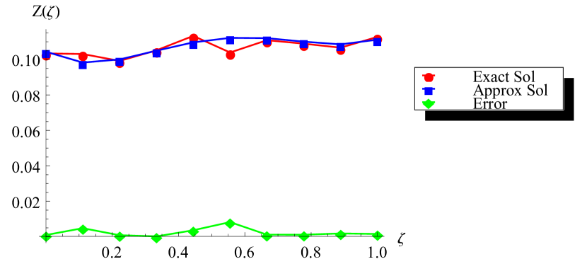
(a) The OCSC method.

(b) The OCSG method.

Figure 1: The exact, approximate and error graphs for $m=4$ (Problem 1).

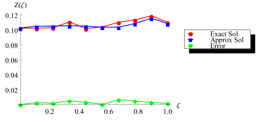
(a) The OCSC method.

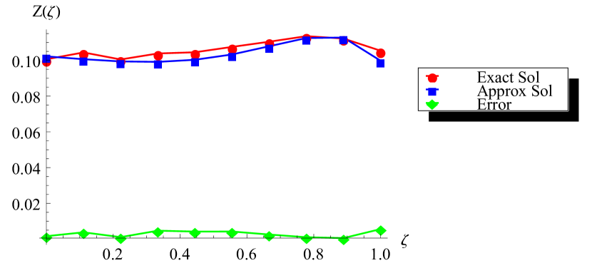
(b) The OCSG method.

Figure 2: The exact, approximate and error graphs for $m=6$ (Problem 1).

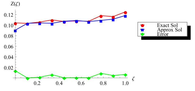
(a) The OCSC method.

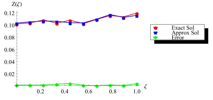
(b) The OCSG method.

Figure 3: The exact, approximate and error graphs for $m=8$ (Problem 1).

Problem 2. Consider the following nonlinear SIVIE :

$$Z(\zeta)=Z_{0}+\alpha^{2}\int_{0}^{\zeta}\cos(Z(\eta))\sin^{3}(Z(\eta))d(\eta)-\alpha\int_{0}^{\zeta}\sin^{2}(Z(\eta))dB(\eta),\quad\zeta,\eta\in[0,1],$$ (5.2)

with the exact solution

$$Z(\zeta)=arc\cot(\alpha B(\zeta)+\cot(Z_{0})),$$

where $\alpha$ and $Z_{0}$ are constants. The numerical methods in sections 3 and 4 have been used to solve this NSIVIE for $\alpha=Z_{0}=\frac{1}{20}$. The exact and approximate solutions are shown in tables 10-15 by two proposed OCSC and OCSG methods respectively. Table 16 provide the comparison between numerical solutions and absolute error by two proposed methods for $m=5$. Figures 4-6 display the absolute error behaviour for various values of $m$ by OCSC method and figures 7-9 represent the absolute error graphs for various values of $m$ by the OCSG method.

Table 10: The OCSC solution for $m=4$ (Problem 2).

$\zeta$	Exact solution	OCSC method solution	Absolute error
0.1	0.0499937	0.0500046	0.0000108944
0.2	0.0499212	0.0499614	0.0000402138
0.3	0.0499242	0.0499878	0.000063579
0.4	0.0498751	0.0500194	0.000144244
0.5	0.0500257	0.0500225	3.16649 $\times 10^{-6}$
0.6	0.0500165	0.049994	0.0000225172
0.7	0.0498062	0.0499615	0.000155243
0.8	0.0500932	0.049983	0.000110212
0.9	0.0500305	0.0501474	0.000116903
1.	0.0501966	0.050574	0.000377446

Table 11: The OCSC solution for $m=6$ (Problem 2).

$\zeta$	Exact solution	OCSC method solution	Absolute error
0.1	0.0500045	0.0500262	0.0000217354
0.2	0.0499019	0.050096	0.000194105
0.3	0.0499859	0.0501041	0.000118166
0.4	0.0500061	0.0499946	0.0000114881
0.5	0.050068	0.04984	0.000228023
0.6	0.0499811	0.0497669	0.000214191
0.7	0.0498003	0.0498647	6.43677$\times 10^{-5}$
0.8	0.0498961	0.0500766	0.000180427
0.9	0.0498414	0.0500724	0.000230957
1.	0.0503336	0.0491044	0.00122919

Table 12: The OCSC solution for $m=8$ (Problem 2).

$\zeta$	Exact solution	OCSC method solution	Absolute error
0.1	0.0499988	0.0505011	0.000502324
0.2	0.0499674	0.0499078	0.00005959
0.3	0.0500501	0.050112	0.0000618491
0.4	0.0499952	0.0500701	0.0000748713
0.5	0.0500326	0.0499367	9.58928$\times 10^{-5}$
0.6	0.0499462	0.050134	0.000187808
0.7	0.0499008	0.0500498	0.000148978
0.8	0.0502124	0.0497176	0.000494796
0.9	0.0499434	0.0505598	0.000616426
1.	0.0501771	0.0440021	0.00617502

Table 13: The OCSG solution for $m=4$ (Problem 2).

$\zeta$	Exact solution	OCSG method solution	Absolute error
0.1	0.0498946	0.0500866	0.000191979
0.2	0.0500082	0.0501338	0.000125616
0.3	0.0500341	0.0501278	0.0000937132
0.4	0.0499708	0.0500954	0.000124622
0.5	0.0498728	0.0500552	0.000182389
0.6	0.0499052	0.0500178	0.000112666
0.7	0.0500471	0.0499858	6.12823$\times 10^{-5}$
0.8	0.0500009	0.0499536	0.0000473285
0.9	0.0502287	0.0499074	0.000321318
1.	0.0500481	0.0498255	0.00022259

Table 14: The OCSG solution for $m=6$ (Problem 2).

$\zeta$	Exact solution	OCSG method solution	Absolute error
0.1	0.0500222	0.0500035	0.0000187625
0.2	0.0499761	0.0499749	$1.23208\times 10^{-6}$
0.3	0.0499805	0.0500212	0.0000406926
0.4	0.0500572	0.0500754	0.0000182051
0.5	0.0499197	0.0500666	0.000146898
0.6	0.0501126	0.0499889	0.000123675
0.7	0.0498796	0.0499116	0.0000319357
0.8	0.0499362	0.0499275	$8.66506\times 10^{-6}$
0.9	0.04993	0.0500431	0.000113119
1.	0.0499052	0.0500068	0.000101627

Table 15: The OCSG solution for $m=8$ (Problem 2).

$\zeta$	Exact solution	OCSG method solution	Absolute error
0.1	0.0500384	0.050103	0.0000645556
0.2	0.050011	0.0499969	0.0000141332
0.3	0.0500499	0.0499871	0.0000627611
0.4	0.0500115	0.0500225	0.0000110429
0.5	0.0500432	0.0499628	8.03721$\times 10^{-5}$
0.6	0.0500414	0.0498371	0.000204304
0.7	0.0499468	0.049844	0.000102772
0.8	0.0500058	0.0500513	0.0000454919
0.9	0.0500509	0.0500969	0.0000460473
1.	0.0498344	0.0495403	0.000294152

Table 16: Comparison of numerical solutions and absolute error between OCSC and OCSG method for, $m=5$ (Problem 2).

$\zeta$	OCSC method		OCSG method
	Numerical solution	Absolute error	Numerical solution	Absolute error
0.1	0.0500365	0.0000464367	0.0499649	0.0000715324
0.2	0.0500887	0.0000867452	0.0499309	0.0000410185
0.3	0.050013	0.0000465181	0.0499386	0.0000691399
0.4	0.0499835	$5.72911\times 10^{-6}$	0.0499931	0.0000136278
0.5	0.0500077	0.0000258911	0.0500653	0.000151897
0.6	0.0500139	0.0000225707	0.0501126	0.000165892
0.7	0.049939	0.000216437	0.0501005	0.000158232
0.8	0.0498153	0.000164775	0.0500239	0.000189945
0.9	0.0498584	0.000318395	0.0499287	0.0000340565
1.0	0.0505544	0.000535273	0.0499324	0.0000831176

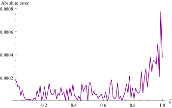
Figure 4: The absolute error graph by OCSC method for $m=4$ (Problem 2).

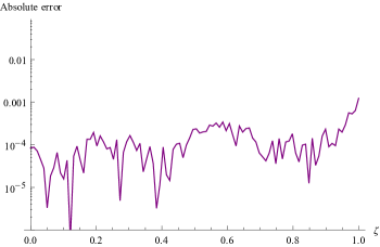
Figure 5: The absolute error graph by OCSC method for $m=6$ (Problem 2).

Figure 6: The absolute error graph by OCSC method for $m=8$ (Problem 2).

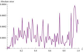
Figure 7: The absolute error graph by OCSG method for $m=4$ (Problem 2).

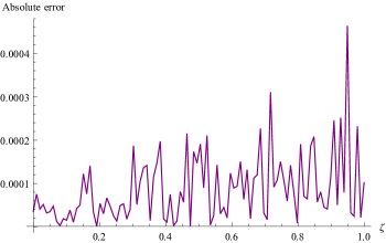
Figure 8: The absolute error graph by OCSG method for $m=6$ (Problem 2).

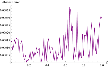
Figure 9: The absolute error graph by OCSG method for $m=8$ (Problem 2).

6 Conclusion

Two novel techniques based on Chelyshkov polynomials are used in this paper to solve the NSIVIE. Using these two methods, the NSIVIE transforms into a set of nonlinear algebraic equations, and by numerically solving these equations, an approximate solution is obtained. In the OCSC method, collocation points have been used, and in the OCSG method, the weak formulation has been implemented numerically by using the inner product based on the orthonormal Chelyshkov polynomial. The convergence analysis of the proposed numerical methods have been presented. Two illustrated examples are presented to demonstrate the accuracy and efficacy of the proposed numerical techniques. The numerical experimental results reveal that there is a good agreement between the approximate solutions obtained by the proposed techniques and the exact solutions.

Declarations

Ethical Approval

Not applicable.

Data Availability

This article includes all the data that were generated or analysed during this research.

Competing interests

The authors assert that there are no competing interests.

Funding

NBHM, Mumbai, under Department of Atomic Energy.

Author’s contribution

All the authors have contributed equally.

References

- [1] Gokme, E., Yuksel G. and Sezer M., 2017, “A numerical approach for solving Volterra type functional integral equations with variable bounds and mixed delays”, Journal of Computational and Applied Mathematics, 311, pp. 354-363.
- [2] Karimi S. and Jozi M., 2015, “A new iterative method for solving linear Fredholm integral equations using the least squares method”, Applied Mathematics and Computation, 250, pp. 744-758.
- [3] Mirzaee F., Hadadiyan E., 2016, “Numerical solution of Volterra–Fredholm integral equations via modification of hat functions”, Applied Mathematics and Computation, 280, pp. 110-123.
- [4] Viggiano B., Friedrich J., Volk R., Bourgoin M., Cal R.B. and Chevillard L., 2020, “ Modelling Lagrangian velocity and acceleration in turbulent flows as infinitely differentiable stochastic processes”, Journal of Fluid Mechanics, 900, p.A27.
- [5] Mao X., Marion G. and Renshaw E., 2002, “ Environmental Brownian noise suppresses explosions in population dynamics”, Stochastic Processes and their Applications, 97(1), pp.95-110.
- [6] Emery A.F., 2004, “ Solving stochastic heat transfer problems”, Engineering Analysis with Boundary Elements, 28(3), pp.279-291.
- [7] Bouchaud J.P. and Sornette D., 1994, “The Black-Scholes option pricing problem in mathematical finance: generalization and extensions for a large class of stochastic processes”, Journal de Physique I, 4(6), pp.863-881.
- [8] Shaw S. and Whiteman J.R., 2000, “Adaptive space–time finite element solution for Volterra equations arising in viscoelasticity problems”, Journal of Computational and Applied Mathematics, 125(1-2), pp.337-345.
- [9] Babaei A., Jafari H., and Banihashemi S., 2020, “A collocation approach for solving time-fractional stochastic heat equation driven by an additive noise”, Symmetry, 12(6), p.904.
- [10] Freund J. A. , Thorsten P., 2000, Stochastic Processes in Physics, Chemistry, and Biology, Springer-Verlag, Berlin.
- [11] Behera S., Saha Ray S., 2020, “An operational matrix based scheme for numerical solutions of nonlinear weakly singular partial integro-differential equations”, Applied Mathematics and Computation, 367, 18 pages.
- [12] Mirzaee F. and Hadadiyan E., 2014, “ A collocation technique for solving nonlinear stochastic Itô–Volterra integral equations”, Applied Mathematics and Computation, 247, pp.1011-1020.
- [13] Wan Z., Chen Y. and Huang Y., 2009, “Legendre spectral Galerkin method for second-kind Volterra integral equations”, Frontiers of Mathematics in China, 4, pp.181-193.
- [14] Yalçinbaş S., 2002, “ Taylor polynomial solutions of nonlinear Volterra–Fredholm integral equations”, Applied Mathematics and Computation, 127(2-3), pp.195-206.
- [15] Maleknejad K., Basirat B. and Hashemizadeh E., 2011, “ Hybrid Legendre polynomials and Block-Pulse functions approach for nonlinear Volterra–Fredholm integro-differential equations”, Computers & Mathematics with applications, 61(9), pp.2821-2828.
- [16] Khajehnasiri A.A., 2016, “ Numerical solution of nonlinear 2D Volterra–Fredholm integro-differential equations by two-dimensional triangular function”, International Journal of Applied and Computational Mathematics, 2, pp.575-591.
- [17] Mohammadi F., 2016, “ Second kind Chebyshev wavelet Galerkin method for stochastic Ito-Volterra integral equations”, Mediterranean Journal of Mathematics, 13, pp.2613-2631.
- [18] Heydari M.H., Hooshmandasl M.R., Ghaini F.M. and Cattani C., 2014, “ A computational method for solving stochastic Itô–Volterra integral equations based on stochastic operational matrix for generalized hat basis functions”, Journal of Computational Physics, 270, pp.402-415.
- [19] Mohammadi, F. and Hosseini, M.M., 2011. A new Legendre wavelet operational matrix of derivative and its applications in solving the singular ordinary differential equations. Journal of the Franklin Institute, 348(8), pp.1787-1796.
- [20] Sahu P.K. and Saha Ray S., 2015, “ A new numerical approach for the solution of nonlinear Fredholm integral equations system of second kind by using Bernstein collocation method”, Mathematical Methods in the Applied Sciences, 38(2), pp.274-280.
- [21] Saha Ray S., Singh P., 2021, “Numerical solution of stochastic Itô-Volterra integral equation by using Shifted Jacobi operational matrix method”, Applied Mathematics and Computation, 410, p.126440.
- [22] Khan S.U., Ali M. and Ali I., 2019, “ A spectral collocation method for stochastic Volterra integro-differential equations and its error analysis”, Advances in Difference Equations, 2019(1), pp.1-14.
- [23] Øksendal B., 2003, “ Stochastic differential equations”, In stochastic differntial equations, Springer, Berlin, Heidelberg, pp. 65-84.
- [24] Heydari M.H., Mahmoudi M.R., Shakiba A. and Avazzadeh Z., 2018, “Chebyshev cardinal wavelets and their application in solving nonlinear stochastic differential equations with fractional Brownian motion”, Communications in Nonlinear Science and Numerical Simulation, 64, pp.98-121.
- [25] Canuto C., Hussaini M.Y., Quarteroni A. and Zang T.A., 2007, “ Spectral methods: fundamentals in single domains”, Springer Science & Business Media.