An ergodic theorem with weights and applications to random measures, RW homogenization and IPS hydrodynamics on point processes

Abstract.

We prove a multidimensional ergodic theorem with weighted averages for the action of the group $\mathbb{Z}^{d}$ on a probability space. At level $n$ weights are of the form $n^{-d}\psi(j/n)$, $j\in\mathbb{Z}^{d}$, for real functions $\psi$ decaying suitably fast. We discuss applications to random measures and to quenched stochastic homogenization of random walks (RWs) on simple point processes with long-range random jump rates, allowing to remove the technical Assumption (A9) from [9, Theorem 4.4]. This last result concerns also some semigroup and resolvent convergence particularly relevant for the derivation of the quenched hydrodynamic limit of interacting particle systems (IPSs) via homogenization and duality. As a consequence we show that also the quenched hydrodynamic limit of the symmetric simple exclusion process on point processes stated in [8, Theorem 4.1] remains valid when removing the above mentioned Assumption (A9).

AMS 2010 Subject Classification: 37A30, 60G55, 60K37, 35B27.

1. Introduction

The multidimensional ergodic theorem with ${\mathbb{Z}}^{d}$–action and arithmetic averages states that, given $d$ commuting measure-preserving and bijective maps $T_{1},T_{2},\dots,T_{d}$ on a probability space $(\Omega,\mathcal{F},{\mathbb{P}})$ and setting $T^{j}:=T_{1}^{j_{1}}\circ T_{2}^{j_{2}}\circ\cdots\circ T_{d}^{j_{d}}$ for $j=(j_{1},j_{2},\dots,j_{d})\in{\mathbb{Z}}^{d}$, the sequence

$$\frac{1}{|I_{n}|}S_{I_{n}}f:=\frac{1}{|I_{n}|}\sum_{j\in I_{n}}f\circ T^{j}$$ (1)

converges as $n\to+\infty$ a.s. and in $L^{p}$ to ${\mathbb{E}}[f|\mathcal{I}]$ for any $f\in L^{p}:=L^{p}(\Omega,\mathcal{F},{\mathbb{P}})$, $p\geq 1$. Above $\mathcal{I}$ is the $\sigma$–algebra of invariant measurable sets and $I_{1}\subset I_{2}\subset I_{3}\subset\cdots$ is any increasing sequence of boxes with union all ${\mathbb{Z}}^{d}$. The above result is due to Tempelman [19] (see e.g. [14, Theorem. 2.8, Chapter 6] and [17, Theorem 2.6]). The multidimensional ergodic theorem can be derived from the maximal inequality (dominated ergodic theorem), which reads ${\mathbb{P}}(|I_{n}|^{-1}S_{I_{n}}f\geq\alpha)\leq C\|f\|_{1}/\alpha$ for any non-negative function $f\in L^{1}$ and $\alpha>0$. The above ergodic theorem has been further generalized by considering more general bounded sets $I_{n}$, by replacing arithmetic averages by weighted averages and also by considering other groups including of course ${\mathbb{R}}^{d}$ (see [14, 17, 19, 20] and the Introduction of [21]).

We are interested here to a generalization of the above multidimensional ergodic theorem for more general averages, where the arithmetic average $|I_{n}|^{-1}S_{I_{n}}f$ is replaced by $\sum_{j\in{\mathbb{Z}}^{d}}c_{n,j}f\circ T^{j}$ for non-negative weights $c_{n,j}$ (non necessarily with bounded support in $j$). We use here the term average in a more relaxed way, not imposing that $c_{n}:=\sum_{j\in{\mathbb{Z}}^{d}}c_{n,j}$ equals $1$ but just that $c_{n}$ converges as $n\to+\infty$ to some $c\in[0,+\infty)$. For the applications motivating our search of such a generalization (see below), the weights $c_{n,j}$ have not bounded support, but decay fast enough as $|j|\to+\infty$.

Several ergodic results for weighted averages are discussed in [14, Chapter 8] (and references therein), mainly for $d=1$. For weights with bounded support we mention the results in [19, Section 7] and [20][Section 4, Chapter 6]. An important contribution for our purposes is given by [21, Proposition 5.3]: for a large class of non-negative measurable functions $\psi$ on ${\mathbb{R}}^{d}$ not necessarily with compact support (e.g. for $\psi$ measurable and such that $0\leq\psi(x)\leq C(1+|x|)^{-\beta}$ with $\beta>d$) given $p\in(1,+\infty)$ and $f\in L^{p}$ the integral $n^{-d}\int_{{\mathbb{R}}^{d}}\psi(x/n)f\circ T^{x}dx$ converges a.s. to ${\color[rgb]{0,0,0}c(\psi)}{\mathbb{E}}[f|\mathcal{I}]$, where $(T^{x})_{x\in{\mathbb{R}}^{d}}$ is an action of the group ${\mathbb{R}}^{d}$ on the probability space, $\mathcal{I}$ is the $\sigma$–algebra of invariant sets and $c(\psi):=\int_{{\mathbb{R}}^{d}}\psi(x)dx$.

In Theorem 2.3 below we present a multidimensional ergodic theorem implying the following. Given the action $(T^{j})_{j\in{\mathbb{Z}}^{d}}$ of ${\mathbb{Z}}^{d}$ on the probability space $(\Omega,\mathcal{F},{\mathbb{P}})$ and given a map $\psi:{\mathbb{R}}^{d}\to{\mathbb{R}}$ with $|\psi(x)|\leq C(1+|x|)^{-\beta}$ and $\beta>2d+2$ (and satisfying some minor conditions), the weighted average $n^{-d}\sum_{j\in{\mathbb{Z}}^{d}}\psi(j/n)f\circ T^{j}$ converges a.s. and in $L^{p}$ as $n\to\infty$ to ${\color[rgb]{0,0,0}c(\psi)}{\mathbb{E}}[f|\mathcal{I}]$ for any $f\in L^{p}$ with $p\in[1,+\infty)$. Although the critical exponent $2d+2$ could not be optimal, this result is enough for our applications and covers the case $p=1$ not covered by [21, Proposition 5.3]. We point out that Theorem 2.3 holds with real weights (i.e. not of fixed sign) and its derivation relies on a maximal inequality (cf. Theorem 2.2).

Our applications concern random measures, stochastic homogenization of random walks on simple point processses and hydrodynamic limits of interacting particle systems on simple point processes. Let us consider the group ${\mathbb{G}}={\mathbb{Z}}^{d}$ or ${\mathbb{G}}={\mathbb{R}}^{d}$ acting on ${\mathbb{R}}^{d}$ by Euclidean translations and on the probability space $(\Omega,\mathcal{F},{\mathbb{P}})$. We assume that ${\mathbb{P}}$ is stationary and ergodic w.r.t. the ${\mathbb{G}}$-action. Let $\mu_{\omega}$ be a random locally finite measure on ${\mathbb{R}}^{d}$ for which a natural covariant relation is satisfied under the two above actions (see Section 3). By calling $\mu^{\varepsilon}_{\omega}$ the rescaled measure $\mu^{\varepsilon}_{\omega}(A):=\varepsilon^{d}\mu_{\omega}(\varepsilon^{-1}A)$, we show that

$$\lim_{\varepsilon\downarrow 0}\int_{{\mathbb{R}}^{d}}\psi(x)\mu^{\varepsilon}_{\omega}(dx)=m\int_{{\mathbb{R}}^{d}}\psi(x)dx\qquad{\mathbb{P}}\text{--a.s.}$$

where $m$ is the intensity of the measure, assumed to be finite, in the following cases where $\psi\in C({\mathbb{R}}^{d})$: (i) $|\psi(x)|\leq C(1+|x|)^{-\beta}$ with $\beta>2d+2$, (ii) $|\psi(x)|\leq C(1+|x|)^{-\beta}$ with $\beta>d$ if in addition for some $\alpha>1$ ${\mathbb{E}}[\mu_{\omega}(A)^{\alpha}]<+\infty$ for any bounded Borel set $A$. The above result has been derived using a tail control related to Theorem 2.3 for case (i) and [21, Proposition 5.3] for case (ii). Note that a priori the measure $\mu_{\omega}$ is not uniformly bounded on balls of fixed radius and density fluctuations can be present with balls with arbitrarly large mass. Hence the above result provides a control at infinity of these fluctuations. In Section 3 we present also further progresses on random measures (see Theorems 3.1 and 3.3, Lemmas 3.2 and 3.4 and Corollary 3.5). For other ergodic results concerning random measures we mention [3, 15, 16] and references therein.

And finally we arrive at our starting motivation. In [9] we have derived quenched stochastic homogenization results for random walks with long-range random jump rates on simple point processes on ${\mathbb{R}}^{d}$ (assuming a stationary and ergodic action of the group ${\mathbb{G}}$). In [8] we have derived the quenched hydrodynamic limit in path space for random walks as above but interacting via site exclusion when the rates are symmetric (the so called symmetric simple exclusion process). Both [8] and [9] aim to universal results applicable to a large class of models. The homogenization in [9] concerns also the convergence of the $L^{2}$-Markov semigroup and resolvent of the random walk towards the corresponding objects of the Brownian motion with diffusion matrix given by the effective homogenized matrix. A suitable form of convergence, also crucial to derive the above mentioned hydrodynamic limit, is derived in [9] under an additional assumption called (A9) in [9], which allows to control at infinity regions where the simple point process has many points. As a consequence the same assumption appears in [8]. Starting from our results for random measures we show that this assumption is not necessary anymore, and the control at infinity is assured by ergodicity. For more details we refer to Section 4 and in particular to Theorem 4.3 and Corollary 4.4. As a consequence, both in [8] and [9] Assumption (A9) can now be removed.

Outline of the paper: In Section 2 we present our multidimensional ergodic theorem with weighted averages (Theorem 2.3) and the associated maximal inequality (Theorem 2.2). In Section 3 we discuss some applications to random measures (Theorems 3.1 and 3.3, Lemmas 3.2 and 3.4 and Corollary 3.5). In Section 4 we discuss applications to random walks with long-range random jump rates on simple point processes (Theorem 4.3) and to the hydrodynamic limit of the symmetric simple exclusion process on simple point processes with random jump rates (Corollary 4.4). The remaining sections are devoted to proofs.

2. An ergodic theorem with weighted averages

We fix some basic notation. We set ${\mathbb{R}}_{+}:=[0,+\infty)$ and ${\mathbb{N}}_{+}:=\{1,2,3,\dots\}$. We denote by $e_{1},e_{2},\dots,e_{d}$ the canonical basis of ${\mathbb{Z}}^{d}$. We fix $\kappa\in[1,+\infty]$ and, given $x\in{\mathbb{R}}^{d}$, we denote by $|x|$ the $\ell^{\kappa}$-norm of $x$ (in particular, $|x|$ is the euclidean norm of $x$ when $\kappa=2$).

Let $T_{1},T_{2},\dots,T_{d}$ be $d$ commuting measure-preserving and bijective maps on a probability space $(\Omega,\mathcal{F},{\mathbb{P}})$. We call $\mathcal{I}\subset\mathcal{F}$ the $\sigma$–subalgebra given by the invariant sets, i.e. $\mathcal{I}:=\{A\in\mathcal{F}\,:\,T_{k}^{-1}A=A\text{ for all }1\leq k\leq d\}$. Moreover we set $T^{j}:=T_{1}^{j_{1}}\circ T_{2}^{j_{2}}\circ\cdots\circ T_{d}^{j_{d}}$ for $j=(j_{1},j_{2},\dots,j_{d})\in{\mathbb{Z}}^{d}$. In what follows we write $L^{p}$ for $L^{p}(\Omega,\mathcal{F},{\mathbb{P}})$ and we denote by ${\mathbb{E}}[\cdot]$ the expectation w.r.t. ${\mathbb{P}}$.

Definition 2.1.

A function $\vartheta:{\mathbb{R}}_{+}\to{\mathbb{R}}_{+}$ is called $d$-good if it is non-increasing and $\sum_{m=0}^{\infty}m^{2d}\vartheta(m)\rho(m)^{-1}<+\infty$ for some positive summable function $\rho:{\mathbb{N}}\to(0,+\infty)$.

Trivially, given $c>0$ and $\beta>2d+2$, the function $\vartheta(r):=c\,(1+r)^{-\beta}$ on ${\mathbb{R}}_{+}$ is $d$-good (take $\rho(m):=(1+m)^{-1-\delta}$ with $\delta>0$ small).

Our first result is the following maximal inequality (see Section 5 for the proof):

Theorem 2.2 (Maximal Inequality).

For any function $\psi:{\mathbb{R}}^{d}\to{\mathbb{R}}_{+}$ such that $\psi(x)\leq\vartheta(|x|)$ for some $d$-good function $\vartheta:{\mathbb{R}}_{+}\to{\mathbb{R}}_{+}$, for any non-negative $f\in L^{1}$ and for any $\alpha>0$, it holds

$${\mathbb{P}}\Big{(}\sup_{n\geq 1}\frac{1}{n^{d}}\sum_{j\in{\mathbb{Z}}^{d}}\psi(j/n)f(T^{j}\omega)>\alpha\Big{)}\leq\frac{C\|f\|_{1}}{\alpha}\,,$$ (2)

where $C=C(d,\vartheta,\rho,\kappa)$ is a suitable positive constant and $\rho$ is as in Definition 2.1.

The above maximal inequality is the main tool to derive the following result (see Section 6 for the proof):

Theorem 2.3 (Ergodic theorem for weighted averages).

Fix a function $\psi:{\mathbb{R}}^{d}\to{\mathbb{R}}$ such that

• $|\psi(x)|\leq\vartheta(|x|)$ for some $d$-good function $\vartheta$;

• $\lim_{n\to+\infty}\frac{1}{n^{d}}\sum_{j\in{\mathbb{Z}}^{d}}|\psi(j/n)-\psi((j+e_{i})/n)|=0$ for any $i=1,..,d$;

• the limit $c(\psi):=\lim_{n\to+\infty}\frac{1}{n^{d}}\sum_{j\in{\mathbb{Z}}^{d}}\psi(j/n)$ exists and is finite.

Then, for any measurable function $f:\Omega\to{\mathbb{R}}$ in $L^{p}$ for some $p\geq 1$, it holds

$$\lim_{n\to+\infty}\frac{1}{n^{d}}\sum_{j\in{\mathbb{Z}}^{d}}\psi(j/n)f(T^{j}\omega)=c(\psi){\mathbb{E}}[f\,|\,\mathcal{I}]$$ (3)

both ${\mathbb{P}}$–a.s. and in $L^{p}$.

Remark 2.4.

If $\psi$ is Riemann integrable, then Item (iii) above holds with $c(\psi):=\int_{{\mathbb{R}}^{d}}\psi(x)dx$. Moreover, the function $\psi(x):=(1+|x|)^{-\beta}$ with $\beta>2d+2$ fullfils all the assumptions of the above ergodic theorem.

We introduce the shorthand notation

$$W^{\psi}_{n}(f)(\omega):=\frac{1}{n^{d}}\sum_{j\in{\mathbb{Z}}^{d}}\psi(j/n)f(T^{j}\omega)\,.$$ (4)

We point out that, whenever $|\psi(x)|\leq\vartheta(|x|)$ for a $d$–good function $\vartheta$, then the series $\frac{1}{n^{d}}\sum_{j\in{\mathbb{Z}}^{d}}\psi(j/n)$ in Item (iii) of Theorem 2.3 is absolutely convergent and therefore well defined. If in addition $f\in L^{p}\subset L^{1}$, then the series defining $W^{\psi}_{n}(f)(\omega)$ is absolutely convergent a.s. Indeed, the measure-preserving property of $T^{j}$ implies that ${\mathbb{E}}[W^{|\psi|}_{n}(|f|)]={\mathbb{E}}[|f|]\frac{1}{n^{d}}\sum_{j\in{\mathbb{Z}}^{d}}|\psi(j/n)|<+\infty$.

3. Applications to random measures on ${\mathbb{R}}^{d}$

Let ${\mathbb{G}}$ be the abelian group ${\mathbb{R}}^{d}$ or ${\mathbb{Z}}^{d}$, endowed with the standard Euclidean topology and the discrete topology, respectively.

We suppose that ${\mathbb{G}}$ acts on the probability space $(\Omega,\mathcal{F},\mathbb{P})$. We call $(\theta_{g})_{g\in{\mathbb{G}}}$ this action. This means that the maps $\theta_{g}:\Omega\to\Omega$ satisfy the following properties: $\theta_{0}=\mathds{1}$; $\theta_{g}\circ\theta_{g^{\prime}}=\theta_{g+g^{\prime}}$ for all $g,g^{\prime}\in{\mathbb{G}}$; the map ${\mathbb{G}}\times\Omega\ni(g,\omega)\mapsto\theta_{g}\omega\in\Omega$ is measurable.

A set $A\in\mathcal{F}$ is called ${\mathbb{G}}$–invariant if $A=\theta_{g}A$ for all $g\in{\mathbb{G}}$.

Assumption $1$: We assume that $\mathbb{P}$ is ${\mathbb{G}}$-stationary, i.e. $\mathbb{P}\circ\theta_{g}^{-1}=\mathbb{P}$ for all $g\in{\mathbb{G}}$. We also assume that $\mathbb{P}$ is ergodic, i.e. $\mathbb{P}(A)\in\{0,1\}$ for any ${\mathbb{G}}$-invariant set $A\in\mathcal{F}$.

We fix a proper action $(\tau_{g})_{g\in{\mathbb{G}}}$ of ${\mathbb{G}}$ on ${\mathbb{R}}^{d}$ given by translations. More precisely, for a given invertible $d\times d$ matrix $V$, we have

$$\tau_{g}x=x+Vg\,,\qquad\forall x\in{\mathbb{R}}^{d}\,,\;\forall g\in{\mathbb{G}}\,.$$ (5)

In several applications $V=\mathbb{I}$, thus implying that $\tau_{g}x=x+g$. The case $V\not=\mathbb{I}$ is particularly relevant when treating e.g. crystal lattices [7, 9].

We denote by $\mathcal{M}$ the metric space of locally finite non-negative measures on ${\mathbb{R}}^{d}$ with $\sigma$–algebra of measurable sets given by the Borel $\sigma$-algebra $\mathcal{B}({\mathbb{R}}^{d})$ [3, Appendix A2.6]. We recall that $\nu_{n}\to\nu$ in $\mathcal{M}$ if and only if $\int_{{\mathbb{R}}^{d}}f(x)d\nu_{n}(x)\to\int_{{\mathbb{R}}^{d}}f(x)d\nu(x)$ for each real continuous function $f$ with compact support (shortly $f\in C_{c}({\mathbb{R}}^{d})$). The action of ${\mathbb{G}}$ on ${\mathbb{R}}^{d}$ naturally induces an action of ${\mathbb{G}}$ on $\mathcal{M}$, which (with some abuse of notation) we still denote by $(\tau_{g})_{g\in{\mathbb{G}}}$. In particular, $\tau_{g}:\mathcal{M}\to\mathcal{M}$ is given by $\tau_{g}\mathfrak{m}(A):=\mathfrak{m}(\tau_{g}A)$ for all $A\in\mathcal{B}({\mathbb{R}}^{d})$ and it holds

$$\int_{{\mathbb{R}}^{d}}f(x)d(\tau_{g}\mathfrak{m})(x)=\int_{{\mathbb{R}}^{d}}f(\tau_{-g}x)d\mathfrak{m}(x)\,.$$ (6)

3.1. ${\mathbb{G}}$–stationary random measure $\mu_{\omega}$ and rescaled random measure $\mu_{\omega}^{\varepsilon}$

We suppose now to have a random locally finite non-negative measure $\mu_{\omega}$ on ${\mathbb{R}}^{d}$, i.e. a measurable map $\Omega\ni\omega\mapsto\mu_{\omega}\in\mathcal{M}$. The fundamental relation between the above two actions of ${\mathbb{G}}$ and the random measure $\mu_{\omega}$ is given by the following assumption:

Assumption $2$: The random measure $\mu_{\omega}$ is ${\mathbb{G}}$–stationary: for all $\omega\in\Omega$ and for all $g\in{\mathbb{G}}$ it holds $\mu_{\theta_{g}\omega}=\tau_{g}\mu_{\omega}$.

Calling $v^{1},v^{2},...,v^{d}$ the columns of $V$, we introduce the parallelepiped

$$\Delta:=\Big{\{}\sum_{i=1}^{d}t_{i}v^{i}\,:\,0\leq t_{i}<1\Big{\}}\,.$$ (7)

When ${\mathbb{G}}={\mathbb{R}}^{d}$ one can also take for $\Delta$ any bounded Borel subset of ${\mathbb{R}}^{d}$ with finite and positive Lebesgue measure (e.g. $\Delta=[0,1)^{d}$). Then the intensity $m$ of the random measure $\mu_{\omega}$ is defined as $m:=\ell(\Delta)^{-1}\int_{\Omega}d\mathbb{P}(\omega)\mu_{\omega}(\Delta)$, where $\ell(\Delta)$ is the Lebesgue measure of $\Delta$. By the ${\mathbb{G}}$–stationarity of $\mathbb{P}$, if ${\mathbb{G}}={\mathbb{R}}^{d}$ then $\int_{\Omega}d\mathbb{P}(\omega)\mu_{\omega}(U)=m\ell(U)$ for any bounded Borel set $U\subset{\mathbb{R}}^{d}$, while if ${\mathbb{G}}={\mathbb{Z}}^{d}$ then $\int_{\Omega}d\mathbb{P}(\omega)\mu_{\omega}(U)=m\ell(U)$ for any bounded set $U$ which is a union of sets of the form $\tau_{g}\Delta$ with $g\in{\mathbb{Z}}^{d}$.

We introduce the rescaled measure $\mu^{\varepsilon}_{\omega}$ defined as

$$\mu^{\varepsilon}_{\omega}(A)=\varepsilon^{d}\mu_{\omega}(\varepsilon^{-1}A)\qquad\forall A\in\mathcal{B}({\mathbb{R}}^{d})\,.$$ (8)

Note that it holds

$$\int_{{\mathbb{R}}^{d}}f(x)d\mu^{\varepsilon}_{\omega}(x)=\varepsilon^{d}\int_{{\mathbb{R}}^{d}}f(\varepsilon x)d\mu_{\omega}(x)$$ (9)

for any Borel function $f:{\mathbb{R}}^{d}\to{\mathbb{R}}_{+}$.

We can now state our limit theorem for $\mu^{\varepsilon}_{\omega}$, where convergence is stronger than the one in $\mathcal{M}$ itself (see Section 7 for the proof):

Theorem 3.1.

Suppose Assumptions $1$ and $2$ to be valid and that the intensity $m$ is finite. Then there exists a ${\mathbb{G}}$–invariant set $\mathcal{A}\subset\Omega$ with $\mathbb{P}(\mathcal{A})=1$ and with the following property. Let $\varphi:{\mathbb{R}}^{d}\to{\mathbb{R}}$ be a continuous function such that, for some $C>0$ and $\beta>2d+2$, $|\varphi(x)|\leq C(1+|x|)^{-\beta}$ for all $x\in{\mathbb{R}}^{d}$. Then for all $\omega\in\mathcal{A}$ the integral $\int_{{\mathbb{R}}^{d}}|\varphi(x)|d\mu^{\varepsilon}_{\omega}(x)$ is finite and it holds

$$\lim_{\varepsilon\downarrow 0}\int_{{\mathbb{R}}^{d}}\varphi(x)d\mu^{\varepsilon}_{\omega}(x)=m\int_{{\mathbb{R}}^{d}}\varphi(x)dx\,.$$ (10)

In particular, (10) holds for all $\omega\in\mathcal{A}$ and all $\varphi$ in the Schwartz space $\mathcal{S}({\mathbb{R}}^{d})$.

The proof of Theorem 3.1 will use the following technical lemma, which will be important also for our applications to stochastic homogenization and hydrodynamics (see Section 7 for the proof):

Lemma 3.2.

Suppose Assumptions $1$ and $2$ to be valid and that the intensity $m$ is finite. Then there exists a ${\mathbb{G}}$–invariant set $\mathcal{C}\subset\Omega$ with $\mathbb{P}(\mathcal{C})=1$ and with the following property. Fixed $\beta>2d+2$ set $\vartheta(r):=(1+r)^{-\beta}$ for $r\geq 0$. Then for all $\omega\in\mathcal{C}$ we have $\int_{{\mathbb{R}}^{d}}\vartheta(|x|)d\mu_{\omega}^{\varepsilon}(x)<+\infty$ and

$$\lim_{\ell\uparrow+\infty}\,\varlimsup_{\varepsilon\downarrow 0}\int_{\{|x|\geq\ell\}}\vartheta(|x|)d\mu_{\omega}^{\varepsilon}(x)=0\,.$$ (11)

When the random measure has higher finite density moments, one can deal with a larger class of functions. Indeed, by means [21, Prop. 5.3] we can derive the following result where $\Delta$ is the fundamental cell defined in (7) (see Section 8 for the proof):

Theorem 3.3.

Suppose Assumptions $1$ and $2$ to be valid. In addition, assume that ${\mathbb{E}}[\mu_{\omega}(\Delta)^{\alpha}]<+\infty$ for some $\alpha>1$. Fix a measurable function $\vartheta:{\mathbb{R}}_{+}\to{\mathbb{R}}_{+}$ such that $\vartheta$ is non-increasing, is convex on $[a,+\infty)$ for some $a>0$ and satisfies $\int_{0}^{\infty}r^{d-1}\vartheta(r)dr<+\infty$. Then there exists a ${\mathbb{G}}$–invariant set ${\color[rgb]{0,0,0}\mathcal{A}_{\vartheta}}\subset\Omega$ with $\mathbb{P}({\color[rgb]{0,0,0}\mathcal{A}_{\vartheta}})=1$ such that, for all $\omega\in{\color[rgb]{0,0,0}\mathcal{A}_{\vartheta}}$, the integral $\int_{{\mathbb{R}}^{d}}|\varphi(x)|d\mu^{\varepsilon}_{\omega}(x)$ is finite and (10) holds for all continuous functions $\varphi:{\mathbb{R}}^{d}\to{\mathbb{R}}$ with $|\varphi(x)|\leq\vartheta(|x|)$.

Trivially, if ${\mathbb{E}}[\mu_{\omega}(\Delta)^{\alpha}]<+\infty$ for some $\alpha>1$, then the intensity $m$ if finite. The proof of the above theorem relies on the following lemma (proved in Section 8), relevant also for our applications to stochastic homogenization and hydrodynamics:

Lemma 3.4.

Suppose Assumptions $1$ and $2$ to be valid. In addition, assume that ${\color[rgb]{0,0,0}{\mathbb{E}}[\mu_{\omega}(\Delta)^{\alpha}]<+\infty}$ for some $\alpha>1$. Fix a function $\vartheta$ as in Theorem 3.3. Then there exists a ${\mathbb{G}}$–invariant set ${\color[rgb]{0,0,0}\mathcal{C}_{\vartheta}}\subset\Omega$ with $\mathbb{P}({\color[rgb]{0,0,0}\mathcal{C}_{\vartheta}})=1$ and such that, for all $\omega\in{\color[rgb]{0,0,0}\mathcal{C}_{\vartheta}}$, it holds $\int_{{\mathbb{R}}^{d}}\vartheta(|x|)d\mu_{\omega}^{\varepsilon}(x)<+\infty$ and (11) is verified.

By applying Theorem 3.3 and Lemma 3.4 to the coutable family of functions $\vartheta:{\mathbb{R}}_{+}\to{\mathbb{R}}_{+}$ of the form $\vartheta(r):=C(1+r)^{-\beta}$ with rational $C,\beta$ and $\beta>d$, one gets the following immediate consequence:

Corollary 3.5.

Suppose Assumptions $1$ and $2$ to be valid. In addition, assume that ${\color[rgb]{0,0,0}{\mathbb{E}}[\mu_{\omega}(\Delta)^{\alpha}]<+\infty}$ for some $\alpha>1$. Then both Theorem 3.1 and Lemma 3.2 remain true if one substitutes the condition $\beta>2d+2$ by the condition $\beta>d$.

Remark 3.6.

For later use we point out that, as the reader can easily check from the proofs, Theorems 3.1 and 3.3, Lemmas 3.2 and 3.4 and Corollary 3.6 remain true if in Assumption $2$ we just require that $\mu_{\theta_{g}\omega}=\tau_{g}\mu_{\omega}$ for all $g\in{\mathbb{G}}$ and all $\omega$ varying in a ${\mathbb{G}}$–invariant set $\Omega_{*}\in\mathcal{F}$ with $\mathbb{P}(\Omega_{*})=1$. We call this version Assumption $2^{*}$ for later use.

4. Application to stochastic homogenization of long-range random walks on point processes and to hydrodynamics

In this section we explain how to extend [9, Theorem 4.4] by removing the restrictive Assumption (A9) present there. In oder to state our final result, we need to recall the setting and some results of [9].

We consider the same setting of the previous section. We assume here that the measure $\mu_{\omega}$ is purely atomic (i.e. pure point) with locally finite support for any $\omega\in\Omega$. In particular, we have

$$\mu_{\omega}=\sum_{x\in\hat{\omega}}n_{x}(\omega)\delta_{x}\,,\;\;\;\;n_{x}(\omega):=\mu_{\omega}(\{x\})\,,\;\;\;\;\hat{\omega}:=\{x\in{\mathbb{R}}^{d}\,:\,n_{x}(\omega)>0\}$$ (12)

and $\hat{\omega}$ is a locally finite set. The map $\omega\mapsto\hat{\omega}$ then defines a simple point process.

We assume to have a measurable function

$$r:\Omega\times{\mathbb{R}}^{d}\times{\mathbb{R}}^{d}\ni(\omega,x,y)\mapsto r_{x,y}(\omega)\in[0,+\infty)\,.$$ (13)

As it will be clear below, only the value of $r_{x,y}(\omega)$ with $x\not=y$ in $\hat{\omega}$ will be relevant. Hence, without loss of generality, we take

$$r_{x,x}(\omega)\equiv 0\,,\qquad r_{x,y}(\omega)\equiv 0\qquad\forall\{x,y\}\not\subset\hat{\omega}\,.$$ (14)

Below $r_{x,y}(\omega)$, with $x,y\in\hat{\omega}$, will be the jump rates of a continuous time random walk in the environment $\omega$ with state space $\hat{\omega}$. Before introducing this random walk we fix some notation and assumptions.

Since we need to deal with the Palm distribution, we need that the intensity $m$ is finite and non zero (if $m$ was zero, $\mu_{\omega}$ would be the zero measure ${\mathbb{P}}$–a.s.). Hence we introduce the following:

Assumption $3$: The intensity $m$ is finite and positive.

We call $\mathbb{P}_{0}$ the Palm distribution associated to $\mathbb{P}$ and the random measure $\mu_{\omega}$. We refer to [9, Section 2.3] and references therein for a detailed exposition. We recall the definition of ${\mathbb{P}}_{0}$.

For ${\mathbb{G}}={\mathbb{R}}^{d}$ and $V={\mathbb{I}}$ the Palm distribution $\mathbb{P}_{0}$ is the probability measure on $(\Omega,\mathcal{F})$ such that, for any $U\in\mathcal{B}({\mathbb{R}}^{d})$ with $0<\ell(U)<\infty$,

$$\mathbb{P}_{0}(A):=\frac{1}{m\ell(U)}\int_{\Omega}d\mathbb{P}(\omega)\int_{U}d\mu_{\omega}(x)\mathds{1}_{A}(\theta_{x}\omega)\,,\qquad\forall A\in\mathcal{F}\,.$$ (15)

$\mathbb{P}_{0}$ has support inside the set $\Omega_{0}:=\{\omega\in\Omega\,:\,n_{0}(\omega)>0\}$. We refer to [9, Section 2.3] for the case ${\mathbb{G}}={\mathbb{R}}^{d}$ and $V$ generic.

For ${\mathbb{G}}={\mathbb{Z}}^{d}$, $V={\mathbb{I}}$, and $\hat{\omega}\subset{\mathbb{Z}}^{d}$ for all $\omega\in\Omega$ (this case will be called special discrete case), the Palm distribution $\mathbb{P}_{0}$ can be identified with the probability measure concentrated on the set $\Omega_{0}:=\{\omega\in\Omega:n_{0}(\omega)>0\}$ such that

$$\mathbb{P}_{0}(A):={\mathbb{E}}\left[n_{0}\,\mathds{1}_{A}\right]/{\mathbb{E}}[n_{0}]\qquad\forall A\in\mathcal{F}\,.$$ (16)

In this particular case the intensity of the random measure is given by $m={\mathbb{E}}[n_{0}]$.

In general, for ${\mathbb{G}}={\mathbb{Z}}^{d}$, the Palm distribution $\mathbb{P}_{0}$ is the probability measure on $\left(\Omega\times\Delta,\mathcal{F}\otimes\mathcal{B}(\Delta)\right)$ (where $\Delta$ is the parallelepiped (7) and $\mathcal{B}(\Delta)$ is its Borel $\sigma$–algebra) such that

$$\mathbb{P}_{0}(A):=\frac{1}{m\,\ell(\Delta)}\int_{\Omega}d\mathbb{P}(\omega)\int_{\Delta}d\mu_{\omega}(x)\mathds{1}_{A}(\omega,x)\,,\qquad\forall A\in\mathcal{F}\otimes\mathcal{B}(\Delta)\,.$$ (17)

$\mathbb{P}_{0}$ has support inside $\Omega_{0}:=\{(\omega,x)\in\Omega\times\Delta\,:\,n_{x}(\omega)>0\}$. In [9] we explain why, in the special discrete case, the above definition reduces (modulo some bijections) to (16).

We define the function $\lambda_{k}:\Omega_{0}\to[0,+\infty]$ (for $k\in[0,\infty)$) as follows:

$$\begin{split}&\begin{cases}\lambda_{k}(\omega):=\sum_{x\in\hat{\omega}}r_{0,x}(\omega)|x|^{k}\\ \Omega_{0}=\{\omega\in\Omega\,:\,n_{0}(\omega)>0\}\end{cases}\qquad\Large{\begin{subarray}{c}\text{\;\;\;\;Case ${\mathbb{G}}={\mathbb{R}}^{d}$ and}\\ \text{\;\;\;\;\;\;\;\;special discrete case}\end{subarray}\,,}\\ &\begin{cases}\lambda_{k}(\omega,a):=\sum_{x\in\hat{\omega}}r_{a,x}(\omega)|x-a|^{k}\\ \Omega_{0}:=\{(\omega,x)\in\Omega\times\Delta\,:\,n_{x}(\omega)>0\}\end{cases}\text{\;Case ${\mathbb{G}}={\mathbb{Z}}^{d}$\,.}\end{split}$$ (18)

Assumption $4$. We assume that for some ${\mathbb{G}}$–invariant set $\Omega_{*}\in\mathcal{F}$ with $\mathbb{P}(\Omega_{*})=1$ the following conditions are fulfilled:

• for all $\omega\in\Omega_{*}$ and $g\not=g^{\prime}$ in ${\mathbb{G}}$, it holds $\theta_{g}\omega\not=\theta_{g^{\prime}}\omega$;

• for all $\omega\in\Omega_{*}$, $g\in{\mathbb{G}}$ and $x,y\in{\mathbb{R}}^{d}$, it holds $r_{x,y}(\theta_{g}\omega)=r_{\tau_{g}x,\tau_{g}y}(\omega)$;

• for all $\omega\in\Omega_{*}$ and $x,y\in{\hat{\omega}}$, it holds $n_{x}(\omega)r_{x,y}(\omega)=n_{y}(\omega)r_{y,x}(\omega)$;

• for all $\omega\in\Omega_{*}$ and $x\not=y$ in $\hat{\omega}$, there exists a path $x=x_{0}$, $x_{1}$,$\dots,x_{n-1},x_{n}=y$ such that $x_{i}\in\hat{\omega}$ and $r_{x_{i},x_{i+1}}(\omega)>0$ for all $i=0,1,\dots,n-1$;

• $\lambda_{0},\lambda_{2}\in L^{1}(\mathbb{P}_{0})$;

• $L^{2}(\mathbb{P}_{0})$ is separable.

Recall Remark 3.6. Assumptions $1$, $2^{*}$, $3$, $4$ correspond to Assumptions (A1),…,(A8) in [9, Section 2] and are satisfied in plenty of models. For examples and comments on the above assumptions we refer to [7, 9].

4.1. The random walk $(X^{\omega}_{t})_{t\geq 0}$ and stochastic homogenization

Given $\omega\in\Omega$, we consider the continuous-time random walk $(X^{\omega}_{t})_{t\geq 0}$ with state space $\hat{\omega}$ and jumping from $x$ to $y\not=x$ with probability rate $r_{x,y}(\omega)$. In particular, once arrived at $x\in\hat{\omega}$ the random walk waits there an exponential time with parameter $r_{x}(\omega):=\sum_{y\in\hat{\omega}}r_{x,y}(\omega)$, afterwards it jumps to another site $y$ in $\hat{\omega}$ chosen with probability $r_{x,y}(\omega)/r_{x}(\omega)$. Due to [9, Lemma 3.5], under general assumptions which are implied by our Assumptions $1$, $2^{*}$, $3$, $4$, (i) the above parameters $r_{x}(\omega)$ are finite and positive for all $x\in\hat{\omega}$ and for ${\mathbb{P}}$–a.a. $\omega$, (ii) the random walk $(X^{\omega}_{t})_{t\geq 0}$ has a.s. no explosion for ${\mathbb{P}}$–a.a. $\omega$ (whatever the starting point) and therefore is well defined for all $t\geq 0$ for $\mathbb{P}$–a.a. $\omega\in\Omega$.

We point out that $(X^{\omega}_{t})_{t\geq 0}$ is a (possibly long-range) random walk on the simple point process $\hat{\omega}$ with $\omega$ sampled by ${\mathbb{P}}$. Our modelling covers several examples, as random walks on supercritical percolation clusters in lattices or in continuum percolation models (as the Boolean model and the random connection model), random walks on crystal lattices, on Delaunay triangulations, on stationary stochastic lattices, Mott’s random walk and so on (see [9, Section 5], [7, Section 3.4], [11] and Figure 1).

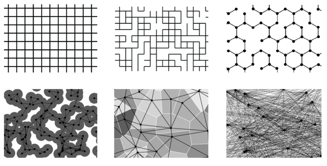
Figure 1. Some random graphs with vertex set $\hat{\omega}$ underlying the random walk $(X^{\omega}_{t})_{t\geq 0}$: lattice ${\mathbb{Z}}^{d}$; the supercritical percolation cluster on ${\mathbb{Z}}^{d}$, on the hexagonal lattice and in the Boolean model; the graph dual to the Voronoi tessellation; a complete graph.

Let $D$ be the effective homogenized matrix. $D$ is implicitly defined as solution of a variational problem, moreover $D$ is a symmetric $d\times d$ positive semidefinite matrix. When $V=\mathbb{I}$, for ${\mathbb{G}}={\mathbb{R}}^{d}$ or in the special discrete case it holds

$$a\cdot Da=\inf_{f\in L^{\infty}(\mathbb{P}_{0})}\frac{1}{2}\int_{\Omega_{0}}d\mathbb{P}_{0}(\omega)\int_{{\mathbb{R}}^{d}}d\hat{\omega}(x)r_{0,x}(\omega)\left(a\cdot x-\nabla f(\omega,x)\right)^{2}\,,$$

for any $a\in{\mathbb{R}}^{d}$, where $\nabla f(\omega,x):=f(\theta_{x}\omega)-f(\omega)$. We refer to [9, Definition 3.6] for the general case. We point out that $D$ can be degenerate and non-zero (see [8, Appendix A] for an example).

Given $\varepsilon>0$ we write $(P^{\varepsilon}_{\omega,t})_{t\geq 0}$ for the $L^{2}(\mu^{\varepsilon}_{\omega})$–Markov semigroup associated to the random walk $(\varepsilon X^{\omega}_{\varepsilon^{-2}t})_{t\geq 0}$ on $\varepsilon\hat{\omega}$, where $\mu^{\varepsilon}_{\omega}:=\varepsilon^{d}\sum_{x\in\hat{\omega}}n_{x}(\omega)\delta_{\varepsilon x}$ according to (8) and (12). Simply, given $f\in L^{2}(\mu^{\varepsilon}_{\omega})$, $P^{\varepsilon}_{\omega,t}f(x)$ is the expectation of $f(\varepsilon X^{\omega}_{\varepsilon^{-2}t})$ when the random walk starts at $\varepsilon x$. We denote by ${\mathbb{L}}^{\varepsilon}_{\omega}$ the infinitesimal generator of the semigroup $(P^{\varepsilon}_{\omega,t})_{t\geq 0}$, which is a self-adjoint operator in $L^{2}(\mu^{\varepsilon}_{\omega})$ (see [9] for more details on ${\mathbb{L}}^{\varepsilon}_{\omega}$). Given $\lambda>0$ we write $R^{\varepsilon}_{\omega,\lambda}:L^{2}(\mu^{\varepsilon}_{\omega})\to L^{2}(\mu^{\varepsilon}_{\omega})$ for the $\lambda$–resolvent associated to the random walk $\varepsilon X^{\omega}_{\varepsilon^{-2}t}$, i.e. $R^{\varepsilon}_{\omega,\lambda}:=(\lambda-{\mathbb{L}}^{\varepsilon}_{\omega})^{-1}=\int_{0}^{\infty}e^{-\lambda s}P^{\varepsilon}_{\omega,s}ds$.

Similarly we write $(P_{t})_{t\geq 0}$ for the Markov semigroup on $L^{2}(mdx)$ associated to the (possibly degenerate) Brownian motion on ${\mathbb{R}}^{d}$ with diffusion matrix $2D$. We denote by $\nabla_{*}$ the weak gradient along the space ${\rm Ker}(D)^{\perp}$ (when $D$ is non-degenerate $\nabla_{*}$ reduces to the standard weak gradient). We write $R_{\lambda}:L^{2}(mdx)\to L^{2}(mdx)$ for the $\lambda$–resolvent associated to the above Brownian motion on ${\mathbb{R}}^{d}$ with diffusion matrix $2D$.

We recall a classical definition in stochastic homogenization:

Definition 4.1.

Fix $\omega\in\Omega$ and a family of $\varepsilon$–parametrized functions $v_{\varepsilon}\in L^{2}(\mu^{\varepsilon}_{\omega})$. The family $\{v_{\varepsilon}\}$ converges weakly to the function $v\in L^{2}(mdx)$ (shortly, $v_{\varepsilon}\rightharpoonup v$) if $\varlimsup_{\varepsilon\downarrow 0}\|v_{\varepsilon}\|_{L^{2}(\mu^{\varepsilon}_{\omega})}<+\infty$ and $\lim_{\varepsilon\downarrow 0}\int_{{\mathbb{R}}^{d}}d\mu^{\varepsilon}_{\omega}(x)v_{\varepsilon}(x)\varphi(x)=\int_{{\mathbb{R}}^{d}}dx\,mv(x)\varphi(x)$ for all $\varphi\in C_{c}({\mathbb{R}}^{d})$. The family $\{v_{\varepsilon}\}$ converges strongly to $v\in L^{2}(mdx)$ (shortly, $v_{\varepsilon}\to v$) if $\varlimsup_{\varepsilon\downarrow 0}\|v_{\varepsilon}\|_{L^{2}(\mu^{\varepsilon}_{\omega})}<+\infty$ and

$$\lim_{\varepsilon\downarrow 0}\int_{{\mathbb{R}}^{d}}d\mu^{\varepsilon}_{\omega}(x)v_{\varepsilon}(x)g_{\varepsilon}(x)=\int_{{\mathbb{R}}^{d}}dx\,mv(x)g(x)$$

for any family of functions $g_{\varepsilon}\in L^{2}(\mu^{\varepsilon}_{\omega})$ weakly converging to $g\in L^{2}(mdx)$.

Remark 4.2.

It is well known, and also recalled in Claim 7.1 in Section 6, that there exists a ${\mathbb{G}}$–invariant set $\mathcal{B}\in\mathcal{F}$ with $\mathbb{P}(\mathcal{B})=1$ such that (10) is true for all functions in $C_{c}({\mathbb{R}}^{d})$. As a consequence, for $\omega\in\mathcal{B}$, strong convergence implies weak convergence.

As stated in [9, Theorem 4.1], under Assumptions $1$, $2^{*}$, $3$, $4$ there exists a ${\mathbb{G}}$–invariant set $\Omega_{\rm typ}\in\mathcal{F}$ with $\mathbb{P}(\Omega_{\rm typ})=1$ such that for all $\omega\in\Omega_{\rm typ}$ and all $\lambda>0$ the massive Poisson equation

$$-{\mathbb{L}}^{\varepsilon}_{\omega}u_{\varepsilon}+\lambda u_{\varepsilon}=f_{\varepsilon}$$ (19)

with $f_{\varepsilon}\in L^{2}(\mu^{\varepsilon}_{\omega})$ stochastically homogenized towards the effective homogenized equation

$$-\nabla_{*}\cdot D\nabla_{*}u+\lambda u=f$$ (20)

with $f\in L^{2}(mdx)$ when $f_{\varepsilon}$ converges (weakly or strongly) to $f$. We refer to [9] for a precise statement of the above homogenization result. Note that (19) and (20) can be rewritten as $u_{\varepsilon}=R^{\varepsilon}_{\omega,\lambda}f_{\varepsilon}$ and $u=R_{\lambda}f$, respectively.

We can now improve [9, Theorem 4.4] in two directions: instead of dealing with functions $f\in C_{c}({\mathbb{R}}^{d})$ we deal with functions vanishing at infinity sufficiently fast and - more importantly - we remove the so called Assumption (A9) from [9, Theorem 4.4] (for our application to hydrodynamic limits indeed it is enough to deal with functions $f\in C_{c}({\mathbb{R}}^{d})$ and the effective advantage is the absence of (A9)). To state the new theorem we set

$$\mathcal{G}(r):=\big{\{}f\in C({\mathbb{R}}^{d})\,:\,\exists C>0,\;\beta>r\text{ with }|f(x)|\leq C(1+|x|)^{-\beta}\;\forall x\in{\mathbb{R}}^{d}\big{\}}\,.$$

Moreover, recall Remark 3.6 and the fundamental cell $\Delta$ introduced in (7).

Theorem 4.3.

Let Assumptions $1$, $2^{*}$, $3$, $4$ be satisfied. Then there exists a measurable set $\Omega^{*}_{\rm typ}\subset\Omega_{\rm typ}$, ${\mathbb{G}}$–invariant and with ${\mathbb{P}}$–probability one, such that as $\varepsilon\downarrow 0$ the following limits hold for any $\omega\in\Omega^{*}_{\rm typ}$, $t\geq 0$, $\lambda>0$ and $f\in\mathcal{S}({\mathbb{R}}^{d})$:

$$L^{2}(\mu^{\varepsilon}_{\omega})\ni P^{\varepsilon}_{\omega,t}f\to P_{t}f\in L^{2}(mdx)\,,$$ (21)

$$L^{2}(\mu^{\varepsilon}_{\omega})\ni R^{\varepsilon}_{\omega,\lambda}f\to R_{\lambda}f\in L^{2}(mdx)\,,$$ (22)

$$\int\bigl{|}P^{\varepsilon}_{\omega,t}f(x)-P_{t}f(x)\bigr{|}^{2}d\mu^{\varepsilon}_{\omega}(x)\to 0\,,$$ (23)

$$\int\bigl{|}R^{\varepsilon}_{\omega,\lambda}f(x)-R_{\lambda}f(x)\bigr{|}^{2}d\mu^{\varepsilon}_{\omega}(x)\to 0\,,$$ (24)

$$\int\bigl{|}P^{\varepsilon}_{\omega,t}f(x)-P_{t}f(x)\bigr{|}d\mu^{\varepsilon}_{\omega}(x)\to 0\,,$$ (25)

$$\int\bigl{|}R^{\varepsilon}_{\omega,\lambda}f(x)-R_{\lambda}f(x)\bigr{|}d\mu^{\varepsilon}_{\omega}(x)\to 0\,.$$ (26)

More specifically, we have

• (21), (22), (23) and (24) hold if $f\in\mathcal{G}(d+1)$; (25) and (26) hold if $f\in\mathcal{G}(2d+2)$;

• if in addition ${\mathbb{E}}\big{[}\mu_{\omega}(\Delta)^{\alpha}]<+\infty$ for some $\alpha>1$, (21), (22), (23) and (24) hold if $f\in\mathcal{G}(d/2)$; (25) and (26) hold $f\in\mathcal{G}(d)$.

The proof of Theorem 4.3 is given in Section 9.

4.2. Hydrodynamics

We conclude by presenting an application of our ergodic Theorem 2.3 to the hydrodynamic limit of interacting particle systems. As discussed in [8] and [9], the limits (25) and (26) are fundamental tools to prove the quenched hydrodynamic behavior of multiple random walks on $\hat{\omega}$ by adding a site exclusion or zero range interaction (combining stochastic homogenization and duality). We refer also to [2, 5, 6, 8, 11, 12, 13] and references therein.

In [8] we have considered the same setting presented above, with $n_{x}(\omega)=1$ and $r_{x,y}(\omega)=r_{y,x}(\omega)$. In this case the random walk $(X_{t}^{\omega})_{t\geq 0}$ on $\hat{\omega}$ becomes a random conductance model on the simple point process $\hat{\omega}$ [1]. Let us consider the associated symmetric simple exclusion process (i.e.  multiple random walks as above interacting by site exclusion). Roughly its Markov generator is given by

$$\mathcal{L}f(\eta):=\sum_{x\in\hat{\omega}}\sum_{y\in\hat{\omega}}r_{x,y}(\omega)\eta(x)(1-\eta(y))\left(f(\eta^{x,y})-f(\eta)\right)\,,$$

where $\eta\in\{0,1\}^{\hat{\omega}}$, $f$ varies in a suitable set of real functions on $\{0,1\}^{\hat{\omega}}$ (including local functions) and $\eta^{x,y}$ is the configuration obtained by exchanging the occupation numbers $\eta(x)$ and $\eta(y)$. Then, under Assumptions (A1),..,(A9) of [9] and the additional Assumption (SEP) (the latter used for the construction of the process and the analysis of its Markov generator), we have derived the quenched hydrodynamic limit in path space for the above symmetric simple exclusion process under diffusive scaling. Assumption (A9) was used to get (25) and (26) from [9] (see [8, Proposition 6.1]). Due to our Theorem 4.3 we then have the following consequence:

Corollary 4.4.

The quenched hydrodynamic limit in path space stated in [8, Theorem 4.1] and described by the hydrodynamic equation $\partial_{t}\rho=\nabla\cdot(D\nabla\rho)$ holds without assuming Assumption (A9) there.

In [11] we will show that also Assumption (SEP) can be removed from [8, Theorem 4.1], hence we refer the interesting reader to [11] for a more detailed discussion.

5. Proof of the Maximal Inequality (Theorem 2.2)

The proof is inspired by the one for the maximal inequality for the action of the group ${\mathbb{Z}}^{d}$ with averages on boxes [14, 17], but we use a different covering procedure in order to control the effects of possible non-zero tails of $\vartheta$.

The following construction and Lemma 5.1 below are a standard tool to prove the maximal inequality. We recall them for completeness since crucial below and since they are usually stated for boxes. Fix $I_{1}\subset I_{2}\subset\cdots\subset I_{N}$ subsets of ${\mathbb{Z}}^{d}$. Suppose to have a finite set $\mathcal{B}\subset{\mathbb{Z}}^{d}$ and a function $k:\mathcal{B}\to\{1,...,N\}$. Define $\mathfrak{m}_{N}$ as a maximal collection of points $z\in\mathcal{B}$ such that $k(z)=N$ and the sets $z+I_{N}$ with $z\in\mathfrak{m}_{N}$ are disjoint. Then define $\mathfrak{m}_{N-1}$ as a maximal collection of points $z\in\mathcal{B}$ such that $k(z)=N-1$ and the sets $z+I_{N-1}$ with $z\in\mathfrak{m}_{N-1}$ are reciprocally disjoint and disjoint from the sets $v+I_{N}$ with $v\in\mathfrak{m}_{N}$. Proceed in this way until defining $\mathfrak{m}_{1}$ as a maximal collection of points $z\in\mathcal{B}$ such that $k(z)=1$ and the sets $z+I_{1}$ with $z\in\mathfrak{m}_{1}$ are reciprocally disjoint and disjoint from the sets $v+I_{k(z)}$ with $v\in\mathfrak{m}_{2}\cup\cdots\cup\mathfrak{m}_{N}$. Finally, we define

$$\mathcal{B}^{\prime}:=\mathfrak{m}_{1}\cup\mathfrak{m}_{2}\cup\cdots\cup\mathfrak{m}_{N}\,.$$

We stress that by construction all sets $z+I_{k(z)}$, $k\in\mathcal{B}^{\prime}$, are disjoint.

Below we use the standard notation $z+A-B:=\{z+a-b\,:\,a\in A\,,\;b\in B\,\}$.

Lemma 5.1.

$\mathcal{B}\subset\cup_{z\in\mathcal{B}^{\prime}}\left(z+I_{k(z)}-I_{k(z)}\right)$ and $|\mathcal{B}|\leq\sum_{z\in\mathcal{B}^{\prime}}|I_{k(z)}-I_{k(z)}|$.

The proof is the same of the proof of [14, Lemma 2.5, Section 6.2].

Proof.

Let us prove that $\mathcal{B}\subset\cup_{z\in\mathcal{B}^{\prime}}\left(z+I_{k(z)}-I_{k(z)}\right)$ (the conclusion then follows immediately). Let $y\in\mathcal{B}$. By the maximality of $\mathfrak{m}_{k(y)}$, there are two possible cases: either $y\in\mathfrak{m}_{k(y)}$ or $y+I_{k(y)}$ intersects some $v+I_{k(v)}$ with $k(v)\geq k(y)$ and $v\in\mathfrak{m}_{k(v)}$ (hence $v\in\mathcal{B}^{\prime}$). In the first case, $y\in\mathcal{B}^{\prime}$ and trivially $y\in y+I_{k(y)}-I_{k(y)}$. In the second case, $\exists a\in I_{k(y)}\subset I_{k(v)}$ and $\exists b\in I_{k(v)}$ such that $y+a=v+b$, thus implying that $y=v+b-a\in v+I_{k(v)}-I_{k(v)}$. ∎

Let $\alpha>0$ and let $N\leq\ell$ be positive integers. All constants of type $c,C$ below have to be thought finite, positive, determined only by $d,\vartheta,{\color[rgb]{0,0,0}\rho},\kappa$ (hence, independent from $\alpha,{\color[rgb]{0,0,0}\ell,N},f$) and can change from line to line.

Recall (4). We define

$$E_{N}(\alpha):=\big{\{}\omega\in\Omega:\sup_{1\leq n\leq N}W^{\psi}_{n}(f)(\omega)>\alpha\big{\}}\,,$$

$$\mathcal{A}(\omega):=\{z\in{\mathbb{Z}}^{d}:|z|\leq\ell\,,\;T^{z}\omega\in E_{N}(\alpha)\}\,.$$

To lighten the notation, sometimes dependence on the parameters will be omitted (as in the definition of $\mathcal{A}(\omega)$, which indeed depends from $\alpha,\ell,N$).

Fix $z\in\mathcal{A}(\omega)$. We know that there exists $k(z)$ with $1\leq k(z)\leq N$ such that $W^{\psi}_{k(z)}(f)(T^{z}\omega)>\alpha$ (in case of multiple possibile indexes $k(z)$, we take e.g. the minimal one). Hence we have

$${\color[rgb]{0,0,0}\alpha k(z)^{d}<k(z)^{d}W^{\psi}_{k(z)}(f)(T^{z}\omega)=}\sum_{j\in{\mathbb{Z}}^{d}}\psi\Big{(}\frac{j-z}{k(z)}\Big{)}f(T^{j}\omega)\qquad\forall z\in\mathcal{A}(\omega)\,.$$ (27)

Let us consider the sets

$${\color[rgb]{0,0,0}D(m,r):=\{x\in{\mathbb{Z}}^{d}\,:\,mr\leq|x|<(m+1)r\}\,,\qquad m\in{\mathbb{N}}\,,\;r=1,2,\dots,N\,.}$$

If $j\in z+D(m,k(z))$, then $mk(z)\leq|j-z|<(m+1)k(z)$, thus implying that $\psi\Big{(}\frac{j-z}{k(z)}\Big{)}\leq\vartheta\Big{(}\frac{|j-z|}{k(z)}\Big{)}\leq\vartheta(m)$ (recall that $\vartheta$ is non-increasing). In particular from (27) and since $\{z+D(m,r):m\in{\mathbb{N}}\}$ is a partition of ${\mathbb{Z}}^{d}$ for any $z\in{\mathbb{Z}}^{d}$ and $r=1,2,\dots,N$, we get

$${\color[rgb]{0,0,0}\alpha k(z)^{d}<}\sum_{m=0}^{{\color[rgb]{0,0,0}+\infty}}\sum_{j\in{\mathbb{Z}}^{d}}\vartheta(m)\mathds{1}_{z+D(m,k(z))}(j)f(T^{j}\omega)\qquad{\color[rgb]{0,0,0}\forall z\in\mathcal{A}(\omega)}\,.$$ (28)

At cost to multiply the function $\rho$ by a positive constant, we can assume that $\sum_{m=0}^{\infty}\rho(m)=1$. Hence, the l.h.s. of (28) can be rewritten as $\sum_{m=0}^{{\color[rgb]{0,0,0}+\infty}}\alpha k(z)^{d}\rho(m)$. As a consequence (recall that $f\geq 0$) there must exist some $m(z)\in{\mathbb{N}}$ such that

$$\alpha k(z)^{d}\rho\big{(}m(z)\big{)}<\sum_{j\in{\mathbb{Z}}^{d}}\vartheta\big{(}m(z)\big{)}\mathds{1}_{D(z)}(j)f(T^{j}\omega)\,,$$ (29)

where $D(z):=z+D\big{(}m(z),k(z)\big{)}$ (in case of many possible $m(z)$’s we take e.g. the minimal one).

For each $m\in{\mathbb{N}}$ we set $\mathcal{A}_{m}(\omega):=\{z\in\mathcal{A}(\omega)\,:\,m(z)=m\}$ and apply Lemma 5.1 with $\mathcal{B}:=\mathcal{A}_{m}(\omega)$, function $k:\mathcal{B}\to\{1,2,\dots,N\}$ as above and sets $I_{1}^{m}\subset I_{2}^{m}\subset\cdots\subset I^{m}_{N}$ given by

$$I^{m}_{r}:=\{x\in{\mathbb{Z}}^{d}\,:\,|x|<(m+1)r\}\qquad r=1,2,\dots,N\,.$$

The construction presented before Lemma 5.1 then produces a subset $\mathcal{A}_{m}^{\prime}(\omega)$ of $\mathcal{A}_{m}(\omega)$ (i.e. $\mathcal{B}^{\prime}=\mathcal{A}_{m}^{\prime}(\omega)$ is the set produced by the construction). By Lemma 5.1 we then have

$$\begin{split}|\mathcal{A}_{m}(\omega)|&\leq\sum_{z\in\mathcal{A}_{m}^{\prime}(\omega)}\Big{|}I^{m}_{k(z)}-I^{m}_{k(z)}\Big{|}\leq c(m+1)^{d}\sum_{z\in\mathcal{A}_{m}^{\prime}(\omega)}k(z)^{d}\\ &=c\frac{(m+1)^{d}}{\alpha{\color[rgb]{0,0,0}\rho}(m)}\sum_{z\in\mathcal{A}_{m}^{\prime}(\omega)}\alpha k(z)^{d}{\color[rgb]{0,0,0}\rho}(m)\,.\end{split}$$ (30)

Above we used that in general $I^{m}_{r}-I^{m}_{r}\subset\{x\in{\mathbb{Z}}^{d}\,:\,|x|<2(m+1)r\}$ which has $c(d,\kappa)(m+1)^{d}r^{d}$ points. As a byproduct of (29) and (30), and since $m(z)=m$ for all $z\in\mathcal{A}^{\prime}_{m}(\omega)\subset{\color[rgb]{0,0,0}\mathcal{A}_{m}(\omega)}$, we have

$$\alpha|\mathcal{A}_{m}(\omega)|<c\frac{(m+1)^{d}}{{\color[rgb]{0,0,0}\rho}(m)}\sum_{z\in\mathcal{A}_{m}^{\prime}(\omega)}\sum_{j\in{\mathbb{Z}}^{d}}\vartheta(m)\mathds{1}_{D(z)}(j)f(T^{j}\omega)\,.$$ (31)

Recall that, given $z\in\mathcal{A}^{\prime}_{m}(\omega){\color[rgb]{0,0,0}\subset\mathcal{A}(\omega)}$, $|z|\leq\ell$ and $k(z)\leq N\leq\ell$. If $j\in D(z)$ and $z\in\mathcal{A}_{m}^{\prime}(\omega)$, then $|j-z|<(m+1)k(z)$, thus implying that $|j|\leq|z|+(m+1)k(z)\leq(m+2)\ell$. In particular, in the r.h.s. of (31) we can restrict to $j\in{\mathbb{Z}}^{d}$ with $|j|\leq(m+2)\ell$. Moreover, by construction the sets $z+I^{m}_{k(z)}$ with $z\in\mathcal{A}_{m}^{\prime}(\omega)$ are disjoint, while $D(z)\subset z+I^{m}_{k(z)}$ for all $z\in\mathcal{A}_{m}^{\prime}(\omega)$. Hence, also all the sets $D(z)$ with $z\in\mathcal{A}_{m}^{\prime}(\omega)$ are disjoint. In particular, given $j\in{\mathbb{Z}}^{d}$ with $|j|\leq(m+2)\ell$, there is at most one $z\in\mathcal{A}_{m}^{\prime}(\omega)$ such that $j\in D(z)$. These observations, the non-negativity of $f$ and (31) lead to

$$\alpha|\mathcal{A}_{m}(\omega)|<c\frac{(m+1)^{d}}{{\color[rgb]{0,0,0}\rho}(m)}\vartheta(m)\sum_{\begin{subarray}{c}j\in{\mathbb{Z}}^{d}:\\ |j|\leq(m+2)\ell\end{subarray}}f(T^{j}\omega)\,.$$ (32)

By taking the expectation of both sides of (32) and using that each $T^{j}$ is measure-preserving we get

$$\alpha{\mathbb{E}}\big{[}|\mathcal{A}_{m}(\omega)|\big{]}\leq c\frac{(m+2)^{2d}}{{\color[rgb]{0,0,0}\rho}(m)}\vartheta(m)\ell^{d}\|f\|_{1}\,.$$ (33)

Summing among all $m\in{\mathbb{N}}$ and using that $\mathcal{A}(\omega)$ is the disjoint union of the $\mathcal{A}_{m}(\omega)$’s, from (33) we get

$$\alpha{\mathbb{E}}\big{[}|\mathcal{A}(\omega)|\big{]}\leq C\ell^{d}\|f\|_{1}\,,\qquad C:=c\sum_{m=0}^{+\infty}\ (m+2)^{2d}\vartheta(m){\color[rgb]{0,0,0}\rho}(m)^{-1}<+\infty$$ (34)

(here we finally use our hypothesis of summability for $\rho$). Since each $T^{z}$ is measure-preserving, we have

$$\begin{split}{\mathbb{E}}\big{[}|\mathcal{A}(\omega)|\big{]}&={\mathbb{E}}[\sum_{z\in{\mathbb{Z}}^{d}:|z|\leq\ell}\mathds{1}\big{(}T^{z}\omega\in E_{N}(\alpha)\big{)}]\\ &=\sum_{z\in{\mathbb{Z}}^{d}:|z|\leq\ell}{\mathbb{P}}\big{(}T^{z}\omega\in E_{N}(\alpha)\big{)}=c\ell^{d}{\mathbb{P}}\big{(}E_{N}(\alpha)\big{)}\,.\end{split}$$ (35)

By combining (34) with (35) we get ${\mathbb{P}}\big{(}E_{N}(\alpha)\big{)}\leq C\|f\|_{1}/\alpha$ for each integer $N\geq 1$ ($\ell$ has disappeared). To conclude the proof and get the maximal inequality (2), it is enough to take the limit $N\to+\infty$ and use the dominated convergence theorem.

6. Proof of the Ergodic Theorem (Theorem 2.3)

We keep a notation very close to the one of the proof of [17, Theorem 2.6] in order to help the comparison. The main structure of the proof is similar. We detail it in order to clarify where the conditions in Items (i), (ii) and (iii) of our Theorem 2.3 are used. Recall our shorthand notation $W^{\psi}_{n}(f)(\omega):=n^{-d}\sum_{j\in{\mathbb{Z}}^{d}}\psi(j/n)f(T^{j}\omega)$.

We call $\tilde{}\mathcal{I}\subset\mathcal{F}$ the $\sigma$–subalgebra given by the almost-invariant sets, i.e. $\tilde{}\mathcal{I}:=\{A\in\mathcal{F}\,:\,{\mathbb{P}}((T_{{\color[rgb]{0,0,0}i}}^{-1}A)\Delta A)=0\text{ for all }1\leq{\color[rgb]{0,0,0}i}\leq d\}$. Trivially, $\mathcal{I}\subset\tilde{}\mathcal{I}$. It is known that, given $A\in\mathcal{F}$, $A\in\tilde{}\mathcal{I}$ if and only if there exists $D\in\mathcal{I}$ such that ${\mathbb{P}}(A\Delta D)=0$ (cf. [4, Exercise 6.1.2-(iii), Chapter 6]). It then follows that ${\mathbb{E}}[f|\mathcal{I}]={\mathbb{E}}[f|\tilde{}\mathcal{I}]$ ${\mathbb{P}}$–a.s. . Hence, we just need to prove Theorem 2.3 with ${\mathbb{E}}[f|\tilde{}\mathcal{I}]$ instead of ${\mathbb{E}}[f|\mathcal{I}]$. In what follows, we call a measurable function $g$ on $\Omega$ invariant if $g\circ T_{i}=g$ ${\mathbb{P}}$–a.s. for all $i=1,2,\dots,d$ (this is equivalent to the fact that $g$ is $\tilde{}\mathcal{I}$–measurable).

As stated and proved in [17, Proof of Theorem 2.6], given $\varepsilon>0$ one can write $f=\sum_{i=1}^{d}(g_{i}-g_{i}\circ T_{i})+h+\varphi$, for suitable functions such that $g_{1},\dots,g_{d}\in L^{\infty}$, $h\in L^{1}$ is $T_{i}$-invariant for all $i=1,2,\dots,d$ (i.e. $h\circ T_{i}=h$ ${\mathbb{P}}$–a.s.) and $\|\varphi\|_{1}<\varepsilon$.

Given a function $u\in L^{1}$, we define the function

$$\Delta(u)(\omega):=\varlimsup_{n\to+\infty}W^{\psi}_{n}(u)(\omega)-\varliminf_{n\to+\infty}W^{\psi}_{n}(u)(\omega)\,.$$

The above limsup and liminf are bounded in modulus by $\sup_{n\geq 1}W_{n}^{|\psi|}(|u|)(\omega)$, which is finite ${\mathbb{P}}$–a.s. by the maximal inequality (applied with $|\psi|$ instead of $\psi$). As a consequence their difference, i.e. $\Delta(u)(\omega)$, is well-defined and finite for ${\mathbb{P}}$-a.a. $\omega$ and in particular for all $\omega\in\Gamma(u)$, where $\Gamma(u):=\{\omega\in\Omega\,:\,\sup_{n\geq 1}W^{|\psi|}_{n}(|u|)(\omega)<+\infty\}$ (note that $\Gamma(u)\in\mathcal{F}$).

$\bullet$ Our first target is to prove that $\Delta(f)(\omega)=0$ for ${\mathbb{P}}$–a.a. $\omega$, thus implying that $\bar{f}(\omega):=\lim_{n\to+\infty}W^{\psi}_{n}{\color[rgb]{0,0,0}(f)}(\omega)$ is well defined and finite for ${\mathbb{P}}$–a.a. $\omega$.

It is simple to check that $\Delta$ is subadditive, i.e. $\Delta(f_{1}+f_{2})(\omega)\leq\Delta(f_{1})(\omega)+\Delta(f_{2})(\omega)$ for all $\omega\in\Gamma(f_{1})\cap\Gamma(f_{2})$. In particular, by writing our $f$ as $f=\sum_{i=1}^{d}(g_{i}-g_{i}\circ T_{i})+h+\varphi$ as above, we have

$$\Delta(f)(\omega)\leq\sum_{i=1}^{d}\Delta(g_{i}-g_{i}\circ T_{i})(\omega)+\Delta(h)(\omega)+\Delta(\varphi)(\omega)$$ (36)

for all $\omega\in\Gamma:=\Gamma(f)\cap\left(\cap_{i=1}^{d}\Gamma(g_{i}-g_{i}\circ T_{i})\right){\color[rgb]{0,0,0}\cap\Gamma(h)}\cap\Gamma(\varphi)$.

We claim that $\Delta(g_{i}-g_{i}\circ T_{i})(\omega)=0$ and $\Delta(h)(\omega)=0$ for ${\mathbb{P}}$–a.a. $\omega$ in $\Gamma$. Let us start with $g_{i}-g_{i}\circ T_{i}$. Since $g_{i}$ is bounded and due to Item (ii) in Theorem 2.3, we get

$$\Big{|}W^{\psi}_{n}(g_{i}-g_{i}\circ T_{i})(\omega)\Big{|}\leq\frac{\|g_{i}\|_{\infty}}{n^{d}}\sum_{j\in{\mathbb{Z}}^{d}}|\psi(j/n)-\psi((j-e_{i})/n)|\stackrel{{\scriptstyle n\to\infty}}{{\rightarrow}}0\,.$$

As a consequence, $\Delta(g_{i}-g_{i}\circ T_{i})(\omega)=0$ for all $\omega\in\Gamma$. Let us move to $\Delta(h)(\omega)$ for $\omega\in\Gamma$. The invariance of $h$ implies that $h(T^{j}\omega)=h(\omega)$ for all $\omega\in\Gamma^{\prime}$, where $\Gamma^{\prime}$ is a measurable set with ${\mathbb{P}}(\Gamma^{\prime})=1$. Due to Item (iii) in Theorem 2.3, we then have

$$W^{\psi}_{n}(h)(\omega)=\frac{h(\omega)}{n^{d}}\sum_{j\in{\mathbb{Z}}^{d}}\psi(j/n)\stackrel{{\scriptstyle n\to\infty}}{{\rightarrow}}c(\psi)h(\omega)\qquad\forall\omega\in\Gamma\cap\Gamma^{\prime}\,.$$ (37)

This implies that $\Delta(h)(\omega)=0$ for all $\omega\in\Gamma\cap\Gamma^{\prime}$, thus concluding the proof of our claim.

As a byproduct of (36) and the above claim, we conclude that $\Delta(f)(\omega)\leq\Delta(\varphi)(\omega)$ for ${\mathbb{P}}$–a.a. $\omega\in\Gamma$. By this observation, the maximal inequality (cf. Theorem 2.2) and since $\|\varphi\|_{1}<\varepsilon$, we have

$$\begin{split}&{\mathbb{P}}(\Delta(f)>\sqrt{\varepsilon})\leq{\mathbb{P}}(\Delta(\varphi)>\sqrt{\varepsilon})\\ &\leq{\mathbb{P}}\Big{(}2\sup_{n\geq 1}\frac{1}{n^{d}}\sum_{j\in{\mathbb{Z}}^{d}}|\psi|(j/n)\,|\varphi|(T^{j}\omega)>\sqrt{\varepsilon}\Big{)}\leq\frac{2C\|\varphi\|_{1}}{\sqrt{\varepsilon}}\leq 2C\sqrt{\varepsilon}\,,\end{split}$$

for some $C=C(d,\vartheta,\rho,\kappa)$. By the arbitrariness of $\varepsilon>0$, we conclude that $\Delta(f)(\omega)=0$ for ${\mathbb{P}}$–a.a. $\omega$.

$\bullet$ We now prove that $\bar{f}$ is invariant, i.e. $\bar{f}=\bar{f}\circ T_{i}$ ${\mathbb{P}}$–a.s. for all $i=1,\dots,d$. By the measure-preserving property of $T_{i}$, the limit $\lim_{n\to+\infty}W^{\psi}_{n}(f)(T_{i}\omega)$ exists and is finte ${\mathbb{P}}$–a.s. and according to our notation it is given by $\bar{f}(T_{i}\omega)$. By the Markov inequality and the measure-preserving property of $T^{j}$ we get

$${\mathbb{P}}(|W^{\psi}_{n}(f)(\omega)-W^{\psi}_{n}(f)(T_{i}\omega)|>\varepsilon)\leq\frac{\|f\|_{1}}{\varepsilon n^{d}}\sum_{j\in{\mathbb{Z}}^{d}}\big{|}\psi(j/n)-\psi((j-e_{i})/n)\big{|}\,.$$ (38)

Since, by Item (ii), $\gamma(n):=n^{-d}\sum_{j\in{\mathbb{Z}}^{d}}\big{|}\psi(j/n)-\psi((j-e_{i})/n)\big{|}\to 0$, for each $k\in{\mathbb{N}}_{+}$ we can find $n_{k}\in{\mathbb{N}}_{+}$ such that $\gamma(n_{k})\leq k^{-3}$ and such that the sequence $n_{k}$ is increasing. At this point, by taking $n=n_{k}$ and $\varepsilon=1/k$ in (38) and afterwards by applying Borel-Cantelli lemma, we conclude that $\lim_{k\to+\infty}\left[W^{\psi}_{n_{k}}(f)(\omega)-W^{\psi}_{n_{k}}(f)(T_{i}\omega)\right]=0$ for ${\mathbb{P}}$–a.a. $\omega$. Since the limit equals $\bar{f}(\omega)-\bar{f}(T_{i}\omega)$ for ${\mathbb{P}}$–a.a. $\omega$, we get that $\bar{f}$ is invariant.

$\bullet$ We now prove that $W_{n}^{\psi}(f)\to\bar{f}$ in $L^{p}$ since $f\in L^{p}$. To this aim, we observe that for $f\in L^{\infty}\cap L^{p}$ this follows from the above proved a.s. convergence $W_{n}^{\psi}(f)\to\bar{f}$ and the dominated convergence theorem (for the latter use that $\|W_{n}^{\psi}(f)\|_{\infty}\leq\|f\|_{\infty}\frac{1}{n^{d}}\sum_{j\in{\mathbb{Z}}^{d}}|\psi(j/n)|$ and the r.h.s. is bounded uniformly in $n$ by Item (iii)). To extend the convergence to any $f\in L^{p}$, we proceed as follows. First we point out that, given $h\in L^{p}$,

$$\|W^{\psi}_{n}(h)\|_{p}\leq\frac{1}{n^{d}}\sum_{j\in{\mathbb{Z}}^{d}}|\psi(j/n)|\,\|h\circ T^{j}\|_{p}=\frac{\|h\|_{p}}{n^{d}}\sum_{j\in{\mathbb{Z}}^{d}}|\psi(j/n)|\leq C\|h\|_{p}\,.$$ (39)

Above, the identity follows from the measure-preserving property of $T^{j}$ and the last bound follows from Item (iii). Given $\delta>0$ let $g\in L^{\infty}\cap L^{p}$ with $\|f-g\|_{p}\leq\delta$ ($g$ exists since $L^{\infty}\cap L^{p}$ is dense in $L^{p}$). By (39) applied to $h=f-g$ and since $W_{n}^{\psi}(g)\to\bar{g}$ in $L^{p}$ we get that $\|W^{\psi}_{n}(f)-\bar{g}\|_{p}\leq 2C\delta$ for $n$ large. By the arbitrariness of $\delta$, this proves that $(W^{\psi}_{n}(f):n\geq 1)$ is a Cauchy sequence in $L^{p}$ and therefore it converges to some $\hat{f}\in L^{p}$. This implies that $W^{\psi}_{n}(f)\to\hat{f}$ ${\mathbb{P}}$–a.s. along a subsequence. Since $W^{\psi}_{n}(f)\to\bar{f}$ ${\mathbb{P}}$–a.s., we conclude that $\hat{f}=\bar{f}$ ${\mathbb{P}}$–a.s. and therefore $W^{\psi}_{n}(f)\to\bar{f}$ in $L^{p}$.

$\bullet$ Finally we prove that $\bar{f}=c(\psi){\mathbb{E}}[f|\tilde{}\mathcal{I}]$ ${\mathbb{P}}$–a.s. To this aim set $a_{n}:=n^{-d}\sum_{j\in{\mathbb{Z}}^{d}}\psi(j/n)$ and take an invariant (i.e. $\tilde{}\mathcal{I}$–measurable) bounded function $g$. Then (using that $g\circ T^{-j}=g$ ${\mathbb{P}}$–a.s. and ${\mathbb{E}}[g|\tilde{}\mathcal{I}]=g$) we get

$$\begin{split}{\mathbb{E}}\left[g{\mathbb{E}}[W^{\psi}_{n}{\color[rgb]{0,0,0}(f)}|\tilde{}\mathcal{I}]\right]&={\mathbb{E}}\left[{\mathbb{E}}[gW^{\psi}_{n}{\color[rgb]{0,0,0}(f)}|\tilde{}\mathcal{I}]\right]={\mathbb{E}}[gW^{\psi}_{n}{\color[rgb]{0,0,0}(f)}]=\frac{1}{n^{d}}\sum_{j\in{\mathbb{Z}}^{d}}\psi(j/n){\mathbb{E}}[g(f\circ T^{j})]\\ &=\frac{1}{n^{d}}\sum_{j\in{\mathbb{Z}}^{d}}\psi(j/n){\mathbb{E}}[(g\circ T^{-j})f]=a_{n}{\mathbb{E}}[gf]=a_{n}{\mathbb{E}}[g{\mathbb{E}}[f|\tilde{}\mathcal{I}]]\,.\end{split}$$

This prove that ${\mathbb{E}}[W^{\psi}_{n}{\color[rgb]{0,0,0}(f)}|\tilde{}\mathcal{I}]=a_{n}{\mathbb{E}}[f|\tilde{}\mathcal{I}]$. We know that $W^{\psi}_{n}{\color[rgb]{0,0,0}(f)}\to\bar{f}\;$ in $L^{p}$. On the other hand, conditional expectation is a contraction in $L^{p}$ (see [4, Therorem 4.1.11, Chapter. 4]), thus implying that ${\mathbb{E}}[W_{n}^{\psi}{\color[rgb]{0,0,0}(f)}|\tilde{}\mathcal{I}]\to{\mathbb{E}}[\bar{f}|\tilde{}\mathcal{I}]$ in $L^{p}$. Since $\bar{f}$ is invariant we have ${\mathbb{E}}[\bar{f}|\tilde{}\mathcal{I}]=\bar{f}$. By combining the above observations we have that $a_{n}{\mathbb{E}}[f|\tilde{}\mathcal{I}]\to\bar{f}$ in $L^{p}$. On the other hand, $a_{n}\to c(\psi)$ by Item (iii) and this allows to conclude that $\bar{f}=c(\psi){\mathbb{E}}[f|\tilde{}\mathcal{I}]$.

7. Applications to random measures: Proof of Theorem 3.1 and Lemma 3.2

In this section we first show how to derive Theorem 3.1 from Lemma 3.2, afterwards we prove the latter. In what follows, given $\ell>0$ we consider the ball $B(\ell):=\{x\in{\mathbb{R}}^{d}\,:\,|x|\leq\ell\}$ and set $B(\ell)^{\rm c}:={\mathbb{R}}^{d}\setminus B(\ell)$.

7.1. Proof of Theorem 3.1

Trivially, it is enough to prove the stated property for the family of rational constants $C>0$ and $\beta>2d+2$. By countability, we just need to prove the statement for a fixed $C>0$ and a fixed $\beta>2d+2$. Without loss of generality we can assume $C=1$. We set $\vartheta(r):=(1+r)^{-\beta}$ for $r\geq 0$ and take $\varphi\in C({\mathbb{R}}^{d})$ with $|\varphi(x)|\leq\vartheta(|x|)$ for all $x\in{\mathbb{R}}^{d}$.

By Lemma 3.2 the integral $\int_{{\mathbb{R}}^{d}}|\varphi(x)|d\mu_{\omega}^{\varepsilon}(x)$ is finite for all $\omega\in\mathcal{C}$. From now on we restrict to $\omega\in\mathcal{C}$. Given a positive $\ell\in{\mathbb{N}}$ take $\varphi_{\ell}\in C_{c}({\mathbb{R}}^{d})$ such that $\varphi_{\ell}=\varphi$ on the ball $B(\ell)$ and $|\varphi_{\ell}(x)|\leq\vartheta(|x|)$ for all $x$. Then, $|\varphi-\varphi_{\ell}|$ is zero on $B(\ell)$ and is bounded by $2\vartheta(|\cdot|)$. This implies that

$$\Big{|}\int_{{\mathbb{R}}^{d}}\varphi(x)d\mu^{\varepsilon}_{\omega}(x)-\int_{{\mathbb{R}}^{d}}\varphi_{\ell}(x)d\mu^{\varepsilon}_{\omega}(x)\Big{|}\leq 2\int_{B(\ell)^{c}}\vartheta(|x|)d\mu^{\varepsilon}_{\omega}(x)$$ (40)

and

$$\Big{|}\int_{{\mathbb{R}}^{d}}\varphi(u)du-\int_{{\mathbb{R}}^{d}}\varphi_{\ell}(u)du\Big{|}\leq 2\int_{B(\ell)^{\rm c}}\vartheta(|u|)du\,.$$ (41)

The last integral goes to zero as $\ell\to+\infty$ since $\vartheta(|\cdot|)$ is integrable on ${\mathbb{R}}^{d}$.

Claim 7.1.

There exists a ${\mathbb{G}}$–invariant set $\mathcal{B}\in\mathcal{F}$ with $\mathbb{P}(\mathcal{B})=1$ such that (10) is true for all functions in $C_{c}({\mathbb{R}}^{d})$.

This fact is usually stated without any proof. Since the derivation is short, we give it for completeness in Appendix A.

Due to Claim 7.1, for all $\ell\in{\mathbb{N}}$ and $\omega\in\mathcal{B}$ we have $\lim_{\varepsilon\downarrow 0}\int_{{\mathbb{R}}^{d}}\varphi_{\ell}(x)d\mu^{\varepsilon}_{\omega}(x)=m\int_{{\mathbb{R}}^{d}}\varphi_{\ell}(x)dx$. By the above observation, (40) and (41) the conclusion follows from Lemma 3.2 and by taking $\mathcal{A}:=\mathcal{B}\cap\mathcal{C}$ with $\mathcal{C}$ as in Lemma 3.2.

7.2. Proof of Lemma 3.2

We set $\psi(x):=\vartheta(|x|)$ and $\psi_{\ell}(x):=\vartheta(|x|)\mathds{1}(|x|\geq\ell)$. Then (11) in Lemma 3.2 follows from

$$\lim_{\ell\uparrow\infty}\,\varlimsup_{\varepsilon\downarrow 0}\int_{{\mathbb{R}}^{d}}\psi_{\ell}(u)d\mu^{\varepsilon}_{\omega}(u)=0\,.$$ (42)

We call $\mathcal{C}$ the set of $\omega\in\Omega$ satisfying (42).

Claim 7.2.

If $\omega\in\mathcal{C}$, then $\int_{{\mathbb{R}}^{d}}\psi(x)d\mu^{\varepsilon}_{\omega}(x)$ is finite for all $\varepsilon>0$.

Proof.

By (9) the above integral equals $\varepsilon^{d}\int_{{\mathbb{R}}^{d}}\psi_{\ell}(\varepsilon u)d\mu_{\omega}(u)$. Hence for $\omega\in\mathcal{C}$ there exists $\ell$ such that $\varepsilon^{d}\int_{{\mathbb{R}}^{d}}\psi_{\ell}(\varepsilon u)d\mu_{\omega}(u)\leq 1$ for $\varepsilon$ small. Since $\mu_{\omega}$ is locally finite, we then have that $\int_{{\mathbb{R}}^{d}}\psi(\varepsilon u)d\mu_{\omega}(u)<+\infty$ for $\varepsilon$ small and our claim follows by observing that the last integral is non-decreasing in $\varepsilon$ as $\vartheta$ is non-increasing. ∎

Claim 7.3.

$\mathcal{C}$ is measurable.

Proof.

Given $\varepsilon,\ell>0$ the map $\Omega\ni\omega\mapsto\int_{{\mathbb{R}}^{d}}\psi_{\ell}(x)d\mu^{\varepsilon}_{\omega}(x)\in{\mathbb{R}}$ is measurable. It is then enough to show that in (42) we can restrict to a countable family of $\ell$ and $\varepsilon$. To this aim, we observe that given $\varepsilon\leq 1$ and $n\in{\mathbb{N}}_{+}$ with $(n+1)^{-1}\leq\varepsilon\leq n^{-1}$, we have (since $\vartheta$ is non-increasing and due to (9))

$$\begin{split}&\int_{{\mathbb{R}}^{d}}\psi_{\ell}(x)d\mu^{\varepsilon}_{\omega}(x)=\varepsilon^{d}\int_{\{\varepsilon|x|\geq\ell\}}\psi(\varepsilon x)dx\leq n^{-d}\int_{\{|x|\geq\ell n\}}\psi(x/(n+1))dx\\ &\leq C(n+1)^{-d}\int_{\{|x|\geq\frac{\ell}{2}(n+1)\}}\psi(x/(n+1))dx=C\int_{{\mathbb{R}}^{d}}\psi_{\frac{\ell}{2}}(x)d\mu^{1/(n+1)}_{\omega}(x)\end{split}$$ (43)

and similarly

$$\begin{split}&\int_{{\mathbb{R}}^{d}}\psi_{\ell}(x)d\mu^{\varepsilon}_{\omega}(x)\geq(n+1)^{-d}\int_{\{|x|\geq\ell(n+1)\}}\psi(x/n)dx\\ &\geq cn^{-d}\int_{\{|x|\geq 2\ell n\}}\psi(x/n)dx=c\int_{{\mathbb{R}}^{d}}\psi_{2\ell}(x)d\mu^{1/n}_{\omega}(x)\,.\end{split}$$ (44)

As a consequence, (42) is equivalent to the same expression but with $\ell\in{\mathbb{N}}$ and $\varepsilon\in\{1/n\,:\,n\in{\mathbb{N}}_{+}\}$. Dealing with a countable family of parameters $\varepsilon,\ell$ one can easily obtain the measurability of $\mathcal{C}$. ∎

Claim 7.4.

$\mathcal{C}$ is ${\mathbb{G}}$-invariant.

Proof.

It is enough to prove that $\forall\omega\in\mathcal{C}$ and $\forall g\in{\mathbb{G}}$ it holds $\theta_{g}\omega\in\mathcal{C}$. Indeed, this means that $\theta_{g}\mathcal{C}\subset\mathcal{C}$ $\forall g\in{\mathbb{G}}$. By applying $\theta_{g}^{-1}=\theta_{-g}$ to both sides, we get $\mathcal{C}\subset\theta_{-g}\mathcal{C}$ $\forall g\in{\mathbb{G}}$, i.e. $\mathcal{C}\subset\theta_{g}\mathcal{C}$ for all $g\in{\mathbb{G}}$. Hence $\theta_{g}\mathcal{C}=\mathcal{C}$ $\forall g\in{\mathbb{G}}$.

Take $\omega\in\mathcal{C}$ and $g\in{\mathbb{G}}$. Due to (6) and (9) we can write

$$\begin{split}\int_{{\mathbb{R}}^{d}}\psi_{\ell}(x)d\mu^{\varepsilon}_{\theta_{g}\omega}(x)&=\int_{\{|x|\geq\ell\}}\psi(x)d\mu^{\varepsilon}_{\theta_{g}\omega}(x)=\varepsilon^{d}\int_{\{|\varepsilon x|\geq\ell\}}\psi(\varepsilon x)d\mu_{\theta_{g}\omega}(x)\\ &=\varepsilon^{d}\int_{\{|\varepsilon(x-Vg)|\geq\ell\}}\psi(\varepsilon(x-Vg))d\mu_{\omega}(x)\,.\end{split}$$ (45)

Since $g$ is fixed, given $\ell>0$, for $\varepsilon$ small we have $|\varepsilon Vg|\leq\ell/2$ and therefore the set $\{x:|\varepsilon(x-Vg)|\geq\ell\}$ is included in the set $\{x:|\varepsilon x|\geq\ell/2\}$. Moreover, for $\varepsilon$ small, we have $|\varepsilon Vg|\leq\ell/4$ and therefore, given $x$ satisfying $|\varepsilon x|\geq\ell/2$, we have $|\varepsilon(x+g)|\geq|(\varepsilon/2)x|$. Since $\vartheta$ is non-increasing, the last bound implies that $\psi(\varepsilon(x+g))\leq\psi((\varepsilon/2)x)$. The above observations and (45) finally imply that

$$\begin{split}&\varlimsup_{\ell\uparrow+\infty}\varlimsup_{\varepsilon\downarrow 0}\int_{{\mathbb{R}}^{d}}\psi_{\ell}(x)d\mu^{\varepsilon}_{\theta_{g}\omega}(x)\leq\\ &\varlimsup_{\ell\uparrow+\infty}\varlimsup_{\varepsilon\downarrow 0}2^{d}(\varepsilon/2)^{d}\int_{\{|(\varepsilon/2)x)|\geq\ell/4\}}\psi((\varepsilon/2)x)d\mu_{\omega}(x)=\\ &2^{d}\varlimsup_{\ell\uparrow+\infty}\varlimsup_{\varepsilon\downarrow 0}\int_{\{|x|\geq\ell/4\}}\psi(x)d\mu^{\varepsilon/2}_{\omega}(x)\,.\end{split}$$

To conclude it is enough to observe that the above r.h.s. is zero since $\omega\in\mathcal{C}$. We have therefore proven that $\theta_{g}\omega\in\mathcal{C}$. ∎

Claim 7.5.

${\mathbb{P}}(\mathcal{C})=1$.

Proof.

For the proof we will apply the ergodic Theorem 2.3. To this aim we let $\Delta(z):=\tau_{z}\Delta$ (recall (7)) and set $f(\omega):=\mu_{\omega}(\Delta)=\mu_{\omega}(\Delta(0))$. Then, by Assumption 2, we have

$$\mu_{\omega}(\Delta(z))=\mu_{\omega}(\tau_{z}\Delta)=\mu_{\theta_{z}\omega}(\Delta)=f(\theta_{z}\omega)\qquad\forall z\in{\mathbb{Z}}^{d}\subset{\mathbb{G}}\,.$$ (46)

Note that $\int_{{\color[rgb]{0,0,0}\Omega}}f(\omega)d{\mathbb{P}}(\omega)=m\ell(\Delta)<+\infty$, hence $f\in L^{1}(\Omega)$. Due to the proof of Claim 7.3, in (42) we can restrict to $\varepsilon$ of the form $1/n$ with $n\in{\mathbb{N}}_{+}$.

$\bullet$ We now want to upper bound the integral in (42) by a weighted average of the random variables $f(\theta_{z}\omega)$ with $z\in{\mathbb{Z}}^{d}$ (producing (50) below). By the form of $\vartheta$ there exists $c>0$ such that

$$\vartheta(r)\leq c\,\vartheta(s)\,\qquad\forall r,s\geq 0\text{ with }|s-r|\leq 1\,.$$ (47)

From now on we restrict to $\varepsilon\leq{\rm diam}(\Delta)^{-1}$, where ${\rm diam}(\Delta)$ denotes the euclidean diameter of $\Delta$. Then, by (47), for $z\in{\mathbb{Z}}^{d}$ and $x\in\Delta(z)$ we can bound $\psi(\varepsilon x)\leq c\,\psi(\varepsilon Vz)$. Indeed, since $\Delta(z)=\tau_{z}\Delta$ and $0\in\Delta$, both $x$ and $\tau_{z}0=Vz$ belong to $\Delta(z)$ and therefore

$$\big{|}\,|\varepsilon x|-|\varepsilon Vz|\,\big{|}\leq\varepsilon|x-Vz|\leq\varepsilon\,{\rm diam}(\Delta)\leq 1\,.$$ (48)

The above bound and (47) allow to conclude that $\psi(\varepsilon x)\leq c\,\psi(\varepsilon Vz)$. By combining this result with the identity $\mu_{\omega}^{\varepsilon}(\varepsilon\Delta(z))=\varepsilon^{d}f(\theta_{z}\omega)$ (which follows from (8) and (46)), we get

$$\int_{\varepsilon\Delta(z)}\psi(u)d\mu^{\varepsilon}_{\omega}(u)\leq c\,\varepsilon^{d}\psi(\varepsilon Vz)f(\theta_{z}\omega)\,.$$ (49)

By (48), if $|\varepsilon x|\geq\ell$ and $x\in\Delta(z)$ then $|\varepsilon Vz|\geq\ell-1$. This observation and (49) imply that

$$\int_{{\mathbb{R}}^{d}}\psi_{\ell}(u)d\mu^{\varepsilon}_{\omega}(u)\leq c\,\varepsilon^{d}\sum_{z\in{\mathbb{Z}}^{d}}\psi_{\ell-1}(\varepsilon Vz)f(\theta_{z}\omega)\,.$$ (50)

$\bullet$ We now want to remove $V$ from (50) in order to deal with a simplified expression (producing (51) below). Since $V$ is invertible, we have $c_{1}|x|\leq|Vx|\leq c_{2}|x|$ for all $x\in{\mathbb{R}}^{d}$ for some constants $c_{1},c_{2}>0$. Hence we have

$$\psi(\varepsilon Vz)\leq(1+\varepsilon c_{1}|z|)^{-\beta}\leq(\min\{1,c_{1}\})^{-\beta}(1+\varepsilon|z|)^{-\beta}=(\min\{1,c_{1}\})^{-\beta}{\color[rgb]{0,0,0}\psi}(\varepsilon z)\,,$$

while $|\varepsilon Vz|\geq\ell-1$ implies $|\varepsilon z|\geq(\ell-1)/c_{2}$. Hence, from (50), we have for some absolute constant $C>0$

$$\int_{{\mathbb{R}}^{d}}\psi_{\ell}(u)d\mu^{\varepsilon}_{\omega}(u)\leq C\,\varepsilon^{d}\sum_{z\in{\mathbb{Z}}^{d}}\psi_{\frac{\ell-1}{c_{2}}}(\varepsilon z)f(\theta_{z}\omega)\,.$$ (51)

Recall that $\varepsilon=1/n$ for some $n\in{\mathbb{N}}_{+}$. Due to (51), (42) is satisfied whenever

$$\lim_{\ell\uparrow\infty}\varlimsup_{n\uparrow\infty}n^{-d}\sum_{z\in{\mathbb{Z}}^{d}}\psi_{\ell}(z/n)f(\theta_{z}\omega)=0\,.$$ (52)

Moreover, since the above integral is decreasing in $\ell$, without loss of generality from now on we restrict to $\ell\in{\mathbb{N}}$.

$\bullet$ We now want to apply the ergodic Theorem 2.3. Let $e_{1},\dots,e_{d}$ be the canonical basis of ${\mathbb{Z}}^{d}$. For $i=1,\dots,d$ we define $T_{i}:\Omega\to\Omega$ as $T_{i}=\theta_{e_{i}}$. Then $T_{1},\dots,T_{d}$ are $d$ commuting measure-preserving bijective maps on $(\Omega,\mathcal{F},\mathbb{P})$ (by Assumption $1$ and since ${\mathbb{Z}}^{d}\subset{\mathbb{G}}$). Moreover the operator $T^{g}:=T_{1}^{g_{1}}\circ T_{2}^{g_{2}}\circ\cdots\circ T_{d}^{g_{d}}$ equals $\theta_{g}$ for all $g=(g_{1},g_{2},\dots,g_{d})\in{\mathbb{Z}}^{d}$. Hence in (52) we can replace $\theta_{z}$ by $T^{z}$. By Theorem 2.3 with $\psi=\psi_{\ell}$ and with $\vartheta(r)=(1+r)^{-\beta}$, $\beta>2d+2$, there exists $\mathcal{C}_{*}\in\mathcal{F}$ with $\mathbb{P}(\mathcal{C}_{*})=1$ such that for all $\omega\in\mathcal{C}_{*}$ the following holds: for each $\ell\in{\mathbb{N}}_{+}$

$$\lim_{n\uparrow+\infty}n^{-d}\sum_{z\in{\mathbb{Z}}^{d}}\psi_{\ell}(\zeta/n)f(\theta_{z}\omega)={\mathbb{E}}[f|\mathcal{I}](\omega)\int\psi_{\ell}(u)du\,,$$ (53)

where $\mathcal{I}:=\{A\in\mathcal{F}\,:\,\theta_{z}A=A\;\;\forall z\in{\mathbb{Z}}^{d}\}$ and ${\mathbb{E}}[f|\mathcal{I}](\omega)$ is a fixed version of the conditional probability of $f$ w.r.t. $\mathcal{I}$. Since the integral in the r.h.s. of (53) goes to zero as $\ell\to+\infty$, we conclude that (52) holds for all $\omega\in\mathcal{C}_{*}$. Since (52) implies (42), we have $\mathcal{C}_{*}\subset\mathcal{C}$, thus implying that ${\mathbb{P}}(\mathcal{C})=1$. ∎

8. Applications to random measures: Proof of Theorem 3.3 and Lemma 3.4

As in the proof of Theorem 3.1, Theorem 3.3 can be derived from Lemma 3.4, which we now focus on. We define $\mathcal{C}_{\vartheta}$ as the set of the $\omega\in\Omega$ satisfying (42) with $\psi(x):=\vartheta(|x|)$ and $\psi_{\ell}(x)=\vartheta(|x|)\mathds{1}(|x|\geq\ell)$. In order to use some proofs of the previous section in what follows we write $\mathcal{C}$ instead of $\mathcal{C}_{\vartheta}$. Then Claims 7.2 and 7.3 are still valid, with the same proofs (we use there only that $\vartheta$ is non-increasing).

It remains to prove Claim 7.5. To this aim we will use [21, Proposition 5.3].

8.1. Proof of Claim 7.5 for ${\mathbb{G}}={\mathbb{R}}^{d}$

We first show that in this case we can assume $V={\mathbb{I}}$ without any loss of generality. To this aim we define $\tilde{\theta}_{g}:=\theta_{V^{-1}g}$ and $\tilde{\tau}_{g}:=\tau_{V^{-1}g}$. Note that $\tilde{\tau}_{g}x=x+V(V^{-1}g)=x+g=x+{\mathbb{I}}g$ and, by Assumption 2,

$$\mu_{\tilde{\theta}_{g}\omega}=\mu_{\theta_{V^{-1}g}\omega}=\tau_{V^{-1}g}\mu_{\omega}=\tilde{\tau}_{g}\mu_{\omega}\,.$$

Since ${\mathbb{G}}={\mathbb{R}}^{d}$ it is then trivial to check that the actions $(\tilde{\theta}_{g})_{g\in{\mathbb{G}}}$ and $(\tilde{\tau}_{g})_{g\in{\mathbb{G}}}$, together with the random measure $\mu_{\omega}$, satisfy Assumptions 1 and 2 and that a set $A\in\mathcal{F}$ is ${\mathbb{G}}$-invariant for the action $(\tilde{\theta}_{g})_{g\in{\mathbb{G}}}$ if and only if the same holds for the action $({\theta}_{g})_{g\in{\mathbb{G}}}$. Then, at cost to pass to the actions $(\tilde{\theta}_{g})_{g\in{\mathbb{G}}}$ and $(\tilde{\tau}_{g})_{g\in{\mathbb{G}}}$, we can (and we do) assume that $V={\mathbb{I}}$.

We fix a smooth function $\gamma:{\mathbb{R}}^{d}\to{\mathbb{R}}_{+}$ with $\gamma(x)$ determined by $|x|$, with support in $B(1):=\{x\in{\mathbb{R}}^{d}\,:\,|x|=1\}$ and satisfying $\int_{{\mathbb{R}}^{d}}\gamma(x)dx=1$. Given $\delta>0$ we consider the mollifier $\gamma_{\delta}(x):=\delta^{d}\gamma(x/\delta)$ (which is a probability kernel with support in $B(\delta)$).

Similarly to the proof of [3, Theorem 10.2.IV] we consider $f:\Omega\to[0,+\infty)$ defined as $f(\omega):=\int_{{\mathbb{R}}^{d}}\gamma_{\delta}(x)d\mu_{\omega}(x)$. Since ${\mathbb{E}}[\mu_{\omega}(B(\delta))^{\alpha}]<+\infty$ (by our moment assumption on $\mu_{\omega}({\color[rgb]{0,0,0}\Delta})$) and $\gamma_{\delta}$ is uniformly bounded, we get that $f\in L^{\alpha}(\Omega)$. In particular, by [21, Proposition 5.3] with $t_{n}:=n$ and by the ergodicity of ${\mathbb{P}}$, there exists a set $\mathcal{C}_{1}\in\mathcal{F}$ such that for all $\omega\in\mathcal{C}_{1}$ it holds

$$\lim_{n\to+\infty}n^{-d}\int_{{\mathbb{R}}^{d}}\vartheta(|x|/n)f(\theta_{x}\omega)dx={\mathbb{E}}[f]\int_{{\mathbb{R}}^{d}}\vartheta(|x|)dx\,.$$ (54)

By stationarity ${\mathbb{E}}[f]=m\int_{{\mathbb{R}}^{d}}\gamma_{\delta}(x)dx=m$. On the other hand, by Assumption 2, we can write (see (6))

$$f(\theta_{x}\omega)=\int_{{\mathbb{R}}^{d}}\gamma_{\delta}(y)d\mu_{\theta_{x}\omega}(y)=\int_{{\mathbb{R}}^{d}}\gamma_{\delta}(y-x)d\mu_{\omega}(y)\,.$$

Setting $z=x-y$ and using also that $\gamma(z)=\gamma(-z)$ we get

$$\begin{split}\int_{{\mathbb{R}}^{d}}\vartheta(|x|/n)f(\theta_{x}\omega)dx&=\int_{{\mathbb{R}}^{d}}dx\,\vartheta(|x|/n)\int_{{\mathbb{R}}^{d}}\gamma_{\delta}(x-y)d\mu_{\omega}(y)\\ &=\int_{{\mathbb{R}}^{d}}d\mu_{\omega}(y)\int_{B(\delta)}\vartheta(|y+z|/n)\gamma_{\delta}(z)dz\,.\end{split}$$ (55)

Since $\vartheta$ is convex on $[a,+\infty)$, the map $x\mapsto\vartheta(|x|)$ is convex on $\{x\in{\mathbb{R}}^{d}\,:\,|x|\geq a\}$. Hence, for $\delta\leq 1$, we have $\int_{B(\delta)}\vartheta(|y+z|/n)\gamma_{\delta}(z)dz\geq\vartheta(|y|/n)$ for $|y|\geq(a+1)n$. On the other hand, by the uniform continuity of $\vartheta$ on $[0,a+2]$, for $n$ large enough we have $\int_{B(\delta)}\vartheta(|y+z|/n)\gamma_{\delta}(z)dz\geq\vartheta(|y|/n)-\delta$ for $|y|\leq(a+1)n$. By combining these bounds with (55) we conclude that

$$\int_{{\mathbb{R}}^{d}}\vartheta(|x|/n)f(\theta_{x}\omega)dx\geq\int_{{\mathbb{R}}^{d}}\vartheta(|y|/n)d\mu_{\omega}(y)-\delta\mu_{\omega}\big{(}B((a+1)n)\big{)}\,.$$ (56)

By Claim 7.1 we have $\ell^{-d}\mu_{\omega}\big{(}B(\ell)\big{)}\to c(d)$ as $\ell\to+\infty$ for any $\omega\in\mathcal{B}$. Hence, by combining (54) with (56) and using that ${\mathbb{E}}[f]=m$, we get for all $\omega\in\mathcal{C}_{1}\cap\mathcal{B}$ and for a positive constant $C={\color[rgb]{0,0,0}C(d,a)}$ that

$$\varlimsup_{n\to+\infty}n^{-d}\int_{{\mathbb{R}}^{d}}\vartheta(|x|/n)d\mu_{\omega}(x)\leq m\int_{{\mathbb{R}}^{d}}\vartheta(|x|)dx+C\delta\,.$$ (57)

Due to the arbitrariness of $\delta$, the above correction $C\delta$ can be removed from (57). Since moreover $\vartheta$ is non-increasing (given $\varepsilon\in(0,1)$ take $n\in{\mathbb{N}}_{+}$ with $(n+1)^{-1}\leq\varepsilon<n^{-1}$), from (57) we get for all $\omega\in\mathcal{C}_{1}\cap\mathcal{B}$ that

$$\varlimsup_{\varepsilon\downarrow 0}\varepsilon^{d}\int_{{\mathbb{R}}^{d}}\vartheta(\varepsilon|x|)d\mu_{\omega}(x)\leq m\int_{{\mathbb{R}}^{d}}\vartheta(|x|)dx\,.$$ (58)

On the other hand, from Claim 7.1 it is trivial to get for any $\omega\in\mathcal{B}$ and any $\ell\in{\mathbb{N}}$ that $\lim_{\varepsilon\downarrow 0}\varepsilon^{d}\int_{{\mathbb{R}}^{d}}\vartheta(\varepsilon|x|)\mathds{1}(\varepsilon|x|<\ell)d\mu_{\omega}(x)=m\int_{\{|x|<\ell\}}\vartheta(|x|)dx$. By subtracting the above limit to (58) and then taking the limit $\ell\uparrow+\infty$, we get

$$\varlimsup_{\ell\uparrow+\infty}\varlimsup_{\varepsilon\downarrow 0}\varepsilon^{d}\int_{\{|\varepsilon x|\geq\ell\}}\vartheta(\varepsilon|x|)d\mu_{\omega}(x){\color[rgb]{0,0,0}\leq m\varlimsup_{\ell\uparrow+\infty}\int_{\{|x|\geq\ell\}}\vartheta(|x|)dx=0}$$ (59)

for any $\omega\in\mathcal{B}\cap\mathcal{C}_{1}$. Note that the equality in (59) is due to the integrability of $\vartheta(|x|)$, which follows from our assumptions. Due to (9), (59) leads to (42). This proves that $\mathcal{C}_{1}\cap\mathcal{B}\subset\mathcal{C}$. Since ${\mathbb{P}}(\mathcal{C}_{1})={\mathbb{P}}(\mathcal{B})=1$, we conclude that ${\mathbb{P}}(\mathcal{C})=1$, thus proving Claim 7.5 for ${\mathbb{G}}={\mathbb{R}}^{d}$.

8.2. Proof of Claim 7.5 for ${\mathbb{G}}={\mathbb{Z}}^{d}$

We move from the action of the group ${\mathbb{Z}}^{d}$ to the action of the group ${\mathbb{R}}^{d}$ by a standard method in homogenization theory. In particular, below we apply the results in [9, Section 6 and Appendix E] (there we treated locally bounded atomic random measures on ${\mathbb{R}}^{d}$, but the results remain valid for generic locally bounded random measures on ${\mathbb{R}}^{d}$). To simplify the presentation and the notation we consider only the case $V={\mathbb{I}}$ (the treatment in [9] is for all $V$). In this case $\Delta=[0,1)^{d}$.

We set $\bar{\Omega}=\Omega\times[0,1)^{d}$ and call $\mathcal{B}$ the Borel $\sigma$–field of $[0,1)^{d}$. We consider the product $\sigma$-algebra $\bar{\mathcal{F}}=\mathcal{F}\otimes\mathcal{B}$ and the product probability measure $\bar{\mathbb{P}}=\mathbb{P}\otimes dx$ on $\bar{\Omega}$. Then $(\bar{\Omega},\bar{\mathcal{F}},\bar{\mathbb{P}})$ is a probability space.

Given $x\in{\mathbb{R}}^{d}$ let $z(x)\in{\mathbb{Z}}^{d}$ and $r(x)\in[0,1)^{d}$ be such that $x=z(x)+r(x)$ (they are univocally defined). Set $\bar{\theta}_{x}:\bar{\Omega}\to\bar{\Omega}$ as $\bar{\theta}_{x}(\omega,a):=(\theta_{z(x+a)}\omega,r(x+a))$. Then one can prove that $(\bar{\theta}_{x})_{x\in{\mathbb{R}}^{d}}$ is a action of ${\mathbb{R}}^{d}$ on $\bar{\Omega}$ and $\bar{\mathbb{P}}$ is stationary and ergodic for this action [9]. In addition, define $\bar{\mu}_{(\omega,a)}(\cdot):=\mu_{\omega}(\cdot+a)$ for all $(\omega,a)\in\bar{\Omega}$. Then we have again the covariant relation $\bar{\mu}_{\theta_{x}(\omega,a)}=\bar{\tau}_{x}\bar{\mu}_{(\omega,a)}$, where $(\bar{\tau}_{x})_{x\in{\mathbb{R}}^{d}}$ is the action of the group ${\mathbb{R}}^{d}$ on the Euclidean space ${\mathbb{R}}^{d}$ by translations $\bar{\tau}_{x}y:=\tau_{x}=y+x$.

In general, due to [9, Section 6], the new setting given by the group $\bar{\mathbb{G}}:={\mathbb{R}}^{d}$, the probability space $(\bar{\Omega},\bar{\mathcal{F}},\bar{\mathbb{P}})$, the actions $(\bar{\theta}_{x})_{x\in\bar{\mathbb{G}}}$ and $(\bar{\tau}_{x})_{x\in\bar{\mathbb{G}}}$, the random measures $\bar{\mu}_{\bar{\omega}}$ with $\bar{\omega}\in\bar{\Omega}$ satisfies Assumptions 1 and 2. Let us show that $\bar{{\mathbb{E}}}[\bar{\mu}_{\bar{\omega}}(\Delta)^{\alpha}]<+\infty$, where $\bar{\mathbb{E}}[\cdot]$ denotes the expectation w.r.t. $\bar{\mathbb{P}}$. This follows from the bound ${\mathbb{E}}[\mu_{\omega}({\color[rgb]{0,0,0}\Delta})^{\alpha}]<+\infty$ and the observation (based also on the stationarity of ${\mathbb{P}}$) that

$$\begin{split}&{\color[rgb]{0,0,0}\bar{{\mathbb{E}}}[\bar{\mu}_{\bar{\omega}}(\Delta)^{\alpha}]=\int_{\Omega}d{\mathbb{P}}(\omega)\int_{\Delta}da\bar{\mu}_{(\omega,a)}(\Delta)^{\alpha}=\int_{\Omega}d{\mathbb{P}}(\omega)\int_{\Delta}da\mu_{\omega}(\Delta+a)^{\alpha}}\\ &{\color[rgb]{0,0,0}=\int_{\Delta}da{\mathbb{E}}[\mu_{\omega}(\Delta+a)^{\alpha}]=\int_{\Delta}da{\mathbb{E}}[\mu_{\omega}(\Delta)^{\alpha}]={\mathbb{E}}[\mu_{\omega}(\Delta)^{\alpha}]}\,.\end{split}$$

In particular the new setting satisfies the assumptions of Lemma 3.4. As a consequence, the result obtained in Section 8.1 implies that there exists a $\bar{\mathbb{G}}$–invariant measurable subset $\bar{}\mathcal{C}\in\bar{}\mathcal{F}$ with $\bar{\mathbb{P}}(\bar{}\mathcal{C})=1$ such that

$$\lim_{\ell\uparrow\infty}\,\varlimsup_{\varepsilon\downarrow 0}\int_{\{|x|\geq\ell\}}\vartheta(|x|)d\bar{\mu}_{(\omega,a)}^{\varepsilon}(x)=0$$

for any $(\omega,a)\in\bar{}\mathcal{C}$. Hence, by the definition of $\bar{\mu}^{\varepsilon}_{(\omega,a)}$ and by (6) and (9), for any $(\omega,a)\in\bar{}\mathcal{C}$ it holds

$$\lim_{\ell\uparrow\infty}\,\varlimsup_{\varepsilon\downarrow 0}\varepsilon^{d}\int_{\{|\varepsilon(x-a)|\geq\ell\}}\vartheta(\varepsilon|x-a|)d\mu_{\omega}(x)=0\,.$$ (60)

We now define $\mathcal{C}_{*}:=\{\omega\in\Omega\,:\,\exists a\in\Delta\text{ with }(\omega,a)\in\bar{}\mathcal{C}\}$. In general, the projection of a measurable subset in a product measure space does not need to be measurable. We can anyway show that $\mathcal{C}_{*}\in\mathcal{F}$ as follows. We know that $\bar{}\mathcal{C}$ is measurable and $\bar{\mathbb{G}}$–invariant. Take $(\omega,a)\in\bar{}\mathcal{C}$ and $a^{\prime}\in\Delta$. Then $\bar{\theta}_{a^{\prime}-a}(\omega,a)=(\theta_{z(a^{\prime})}\omega,r(a^{\prime}))=(\theta_{0}\omega,a^{\prime})=(\omega,a^{\prime})$. This observation and the $\bar{\mathbb{G}}$-invariance of $\bar{}\mathcal{C}$ imply that $(\omega,a^{\prime})\in\bar{}\mathcal{C}$ for any $(\omega,a)\in\bar{}\mathcal{C}$. Hence, $\bar{}\mathcal{C}=\mathcal{C}_{*}\times\Delta$. Since sections are measurable (see [18, Exercise 1.7.18-(iii)]) we conclude that $\mathcal{C}_{*}$ is measurable, i.e. $\mathcal{C}_{*}\in\mathcal{F}$. Moreover, since $\bar{\mathbb{P}}(\bar{}\mathcal{C})=1$, it must be ${\mathbb{P}}(\mathcal{C}_{*})=1$ by Fubini-Tonelli Theorem.

At this point, to conclude the proof of Claim 7.5 (i.e. ${\mathbb{P}}(\mathcal{C})=1$), it remains to show that $\mathcal{C}_{*}\subset\mathcal{C}$. To this aim we take $\omega\in\mathcal{C}_{*}$. We know that (60) holds for any $a\in\Delta$. By taking $a=0$, (60) reduces to (42).

9. Proof of Theorem 4.3

We prove Items (i) and (ii) of Theorem 4.3. Item (i) trivially implies the result for $\mathcal{S}({\mathbb{R}}^{d})$.

Let $\mathcal{B}$ be as in Remark 4.2 and Claim 7.1 For Item (i) we define $d_{c}:=2d+2$ and $\Omega_{\rm typ}^{*}\in\mathcal{F}$ as $\Omega^{*}_{\rm typ}:=\Omega_{\rm typ}\cap\mathcal{A}\cap\mathcal{B}\cap\mathcal{C}$, where $\mathcal{A}$ and $\mathcal{C}$ are as in Theorem 3.1 and Lemma 3.2 respectively. For Item (ii) we define $d_{c}:=d$ and $\Omega_{\rm typ}^{*}\in\mathcal{F}$ as $\Omega^{*}_{\rm typ}:=\Omega_{\rm typ}\cap\mathcal{A}\cap\mathcal{B}\cap\mathcal{C}$, where $\mathcal{A}$ and $\mathcal{C}$ are as in Corollary 3.5. Note that $\Omega^{*}_{\rm typ}$ is measurable, ${\mathbb{G}}$–invariant and ${\mathbb{P}}(\Omega_{\rm typ}^{*})=1$. From now on we restrict to $\omega\in\Omega^{*}_{\rm typ}$.

By Theorem 3.1 and Corollary 3.5, for any $f\in\mathcal{G}(d_{c}/2)$ we get that $f\in L^{2}(\mu^{\varepsilon}_{\omega})$ and $\|f\|_{L^{2}(\mu^{\varepsilon}_{\omega})}^{2}=\int_{{\mathbb{R}}^{d}}f(x)^{2}d\mu^{\varepsilon}_{\omega}(x)$ converges to $\|f\|^{2}_{L^{2}(mdx)}=m\int_{{\mathbb{R}}^{d}}f(x)^{2}dx$ as $\varepsilon\downarrow 0$. We claim that we also have $L^{2}(\mu^{\varepsilon}_{\omega})\ni f\mapsto f\in L^{2}(mdx)$ as $\varepsilon\downarrow 0$. Having just proved the convergence of norms, to prove this strong convergence it is enough to prove the weak convergence $L^{2}(\mu^{\varepsilon}_{\omega})\ni f\rightharpoonup f\in L^{2}(mdx)$ (see e.g. [9, Remark 3.12]). Since $f\psi\in C_{c}({\mathbb{R}}^{d})$ for any $\psi\in C_{c}({\mathbb{R}}^{d})$, this weak convergence follows again from Theorem 3.1 (Claim 7.1 would be enough).

By combining the above strong convergence $L^{2}(\mu^{\varepsilon}_{\omega})\ni f\mapsto f\in L^{2}(mdx)$ with [9, Theorem 4.1–(i)], we get (22) for $f\in\mathcal{G}(d_{c}/2)$. Then (21) for $f\in\mathcal{G}(d_{c}/2)$ follows from (22) and [22, Theorem 9.2].

Claim 9.1.

Let $f$ be a measurable bounded function. Let $t\geq 0$ and $\lambda>0$. If for some $C,\beta>0$ it holds $|f(x)|\leq C(1+|x|)^{-\beta}$ for all $x\in{\mathbb{R}}^{d}$, then for some $C^{\prime}$ it holds $|P_{t}f(x)|\leq C^{\prime}(1+|x|)^{-\beta}$ and $|R_{\lambda}f(x)|\leq C^{\prime}(1+|x|)^{-\beta}$ for all $x\in{\mathbb{R}}^{d}$.

Proof.

The proof follows by simple computations, based on estimates in the same spirit of the following ones. Below constants of type $c$ are positive and can change from line to line. Fix $\beta>0$. Given $t>0$ and working in ${\mathbb{R}}^{k}$ with $1\leq k\leq d$, let

$$C(x,t):=t^{-\frac{k}{2}}\int_{{\mathbb{R}}^{k}}e^{-\frac{|x-y|^{2}}{t}}(1+|y|)^{-\beta}dy\,,$$

$$C_{1}(x,t):=t^{-\frac{k}{2}}\int_{\{|y|\leq|x|/2\}}e^{-\frac{|x-y|^{2}}{t}}(1+|y|)^{-\beta}dy\,,$$

$$C_{2}(x,t):=t^{-\frac{k}{2}}\int_{\{|y|>|x|/2\}}e^{-\frac{|x-y|^{2}}{t}}(1+|y|)^{-\beta}dy\,.$$

Then $C(x,t)=C_{1}(x,t)+C_{2}(x,t)$ and

$$C_{1}(x,t)\leq t^{-\frac{k}{2}}e^{-\frac{|x|^{2}}{4t}}\int_{\{|y|\leq|x|/2\}}1dy\leq ct^{-\frac{k}{2}}e^{-\frac{|x|^{2}}{4t}}(1+|x|)^{k}\,,$$ (61)

$$C_{2}(x,t)\leq(1+|x|/2)^{-\beta}t^{-\frac{k}{2}}\int_{{\mathbb{R}}^{k}}e^{-\frac{|x-y|^{2}}{t}}dx\leq c(1+|x|)^{-\beta}\,.$$ (62)

When $t=1$, we get $C(x,t)\leq c(1+|x|)^{-\beta}$. Reasoning similarly (by bounding $P_{t}f(x)$ by an integral similar to $C(x,1)$), we get the claim for $P_{t}f(x)$.

We move to the resolvent. Since $R_{\lambda}f(x)=\int_{0}^{\infty}e^{-\lambda t}P_{t}f(x)dt$, we have $\|R_{\lambda}\|_{\infty}\leq\|f\|_{\infty}/\lambda$. Hence, to prove that $|R_{\lambda}f(x)|\leq C^{\prime}(1+|x|)^{-\beta}$, we can restrict to $|x|$ large enough.

Let us take $|x|\geq 1$. We can bound $\int_{0}^{\infty}e^{-\lambda t}t^{-\frac{k}{2}}e^{-\frac{|x|^{2}}{4t}}dt$ by treating separately the integral over $\{t>|x|\}$ and the integral over $\{0\leq t\leq|x|\}$. The former is bounded by $\int_{|x|}^{\infty}e^{-\lambda t}dt=e^{-\|x\|}/\lambda$. The latter is bounded by $e^{-\frac{|x|}{8}}\int_{0}^{|x|}t^{-\frac{k}{2}}e^{-\frac{|x|^{2}}{8t}}dt$, which for $|x|\geq 1$ is bounded by

$$e^{-\frac{|x|}{8}}|x|^{-k}\int_{0}^{|x|}(t/|x|^{2})^{-\frac{k}{2}}e^{-\frac{|x|^{2}}{8t}}dt\leq ce^{-\frac{|x|}{8}}|x|^{1-2k}$$

(we have used that $s^{-\frac{k}{2}}e^{-\frac{1}{8s}}$ is bounded on ${\mathbb{R}}_{+}$).

By combining the above bounds with (61) and (62) we get $\int_{0}^{\infty}e^{-\lambda t}C(x,t)dt\leq c(1+|x|)^{-\beta}$ for $|x|\geq 1$. By similar computations one can prove that $|\mathcal{R}_{\lambda}f(x)|\leq C^{\prime}(1+|x|)^{-\beta}$ for $|x|$ large.

∎

The following claim and the related proof are similar to [5, Lemma 6.1] and its proof, respectively.

Claim 9.2.

Given $h\in{\color[rgb]{0,0,0}\mathcal{G}(d_{c}/2)}$ and given a family $h^{\varepsilon}_{\omega}\in L^{2}(\mu^{\varepsilon}_{\omega})$ with $L^{2}(\mu^{\varepsilon}_{\omega})\ni h^{\varepsilon}_{\omega}\to h\in L^{2}(mdx)$, it holds $\lim_{\varepsilon\downarrow 0}\int_{{\mathbb{R}}^{d}}|h^{\varepsilon}_{\omega}(x)-h(x)|^{2}d\mu^{\varepsilon}_{\omega}(x)=0$.

Proof.

Since ${\color[rgb]{0,0,0}h\in\mathcal{G}(d_{c}/2)}$ and by Theorem 3.1 and Corollary 3.5, we have $\int_{{\mathbb{R}}^{d}}h(x)^{2}d\mu^{\varepsilon}_{\omega}(x)\to m\int_{{\mathbb{R}}^{d}}h(x)^{2}dx$ as $\varepsilon\downarrow 0$. Let us show that $\int_{{\mathbb{R}}^{d}}h^{\varepsilon}_{\omega}(x)^{2}d\mu^{\varepsilon}_{\omega}(x)\to m\int_{{\mathbb{R}}^{d}}h(x)^{2}dx$. To get this limit it is enough to observe that, by Remark 4.2, $h^{\varepsilon}_{\omega}\rightharpoonup h$ and this allows to take $g_{\varepsilon}:=h^{\varepsilon}_{\omega}$ and $g:=h$ when applying Definition 4.1 to the strong convergence $L^{2}(\mu^{\varepsilon}_{\omega})\ni h^{\varepsilon}_{\omega}\to h\in L^{2}(mdx)$. This implies that $\int_{{\mathbb{R}}^{d}}h^{\varepsilon}_{\omega}(x)^{2}d\mu^{\varepsilon}_{\omega}(x)\to m\int_{{\mathbb{R}}^{d}}h(x)^{2}dx$.

As $\int_{{\mathbb{R}}^{d}}h(x)^{2}d\mu^{\varepsilon}_{\omega}(x)\to m\int_{{\mathbb{R}}^{d}}h(x)^{2}dx$ and $\int_{{\mathbb{R}}^{d}}h^{\varepsilon}_{\omega}(x)^{2}d\mu^{\varepsilon}_{\omega}(x)\to m\int_{{\mathbb{R}}^{d}}h(x)^{2}dx$, to conclude the proof of our claim we show that $\int_{{\mathbb{R}}^{d}}h^{\varepsilon}_{\omega}(x)h(x)d\mu^{\varepsilon}_{\omega}(x)\to m\int_{{\mathbb{R}}^{d}}h(x)^{2}dx$. Since $h\in\mathcal{G}(d_{c}/2)$ we have $|h(x)|\leq C(1+|x|)^{-\beta}$ for all $x\in{\mathbb{R}}^{d}$, for some $C>0$ and $\beta>d_{c}/2$. Given an integer $\ell>0$ we fix a function $g_{\ell}\in C_{c}({\mathbb{R}}^{d})$ such that $g_{\ell}(x)=h(x)$ for $|x|\leq\ell$ and $|g_{\ell}(x)|\leq C(1+|x|)^{-\beta}$ for all $x\in{\mathbb{R}}^{d}$. Then, using the weak convergence $h^{\varepsilon}_{\omega}\rightharpoonup h$, we get

$$\lim_{\varepsilon\downarrow 0}\int_{{\mathbb{R}}^{d}}h^{\varepsilon}_{\omega}(x)g_{\ell}(x)d\mu^{\varepsilon}_{\omega}(x)=m\int_{{\mathbb{R}}^{d}}h(x)g_{\ell}(x)dx\,,$$

which trivially implies that

$$\lim_{\ell\uparrow+\infty}\lim_{\varepsilon\downarrow 0}\int_{{\mathbb{R}}^{d}}h^{\varepsilon}_{\omega}(x)g_{\ell}(x)d\mu^{\varepsilon}_{\omega}(x)=m\int_{{\mathbb{R}}^{d}}h(x)^{2}dx\,.$$ (63)

On the other hand, by Schwarz inequality and our bounds on $h$ and $g_{\ell}$ and recalling that $B(\ell):=\{x\in{\mathbb{R}}^{d}\,:\,|x|\leq\ell\}$, we can estimate

$$\begin{split}\Big{|}\int_{{\mathbb{R}}^{d}}h^{\varepsilon}_{\omega}(x)\bigl{(}h(x)-g_{\ell}(x)\bigr{)}d\mu^{\varepsilon}_{\omega}(x)\Big{|}&\leq\|h^{\varepsilon}_{\omega}\|_{L^{2}(\mu^{\varepsilon}_{\omega})}\|h(x)-g_{\ell}(x)\|_{L^{2}(\mu^{\varepsilon}_{\omega})}\\ &\leq 2C\|h^{\varepsilon}_{\omega}\|_{L^{2}(\mu^{\varepsilon}_{\omega})}\|\mathds{1}_{B(\ell)}(x)(1+|x|)^{-\beta}\|_{L^{2}(\mu^{\varepsilon}_{\omega})}\,.\end{split}$$

By the above estimate, Lemma 3.2 and Corollary 3.5 and since $\varlimsup_{\varepsilon\downarrow 0}\|h^{\varepsilon}_{\omega}\|_{L^{2}(\mu^{\varepsilon}_{\omega})}<+\infty$ by assumption, we conclude that

$$\lim_{\ell\uparrow+\infty}\varlimsup_{\varepsilon\downarrow 0}\Big{|}\int_{{\mathbb{R}}^{d}}h^{\varepsilon}_{\omega}(x)\bigl{(}h(x)-g_{\ell}(x)\bigr{)}d\mu^{\varepsilon}_{\omega}(x)\Big{|}=0\,.$$ (64)

To conclude it is now enough to combine (63) and (64). ∎

Let $f\in\mathcal{G}(d_{c}/2)$. We can apply Claim 9.2 with $h_{\omega}^{\varepsilon}:=P^{\varepsilon}_{\omega,t}f$ and $h=P_{t}f$. Indeed, we know that $P_{t}f\in\mathcal{G}(d_{c}/2)$ by Claim 9.1 and we know that $L^{2}(\mu^{\varepsilon}_{\omega})\ni h^{\varepsilon}_{\omega}\to h\in L^{2}(mdx)$ by (21). Then by Claim 9.2 we get (23). By the same arguments, and using now (22), we get (24).

It remains to prove (25) and (26) for $f\in\mathcal{G}(d_{c})$. Let us prove (26). Without loss of generality one can take $f\geq 0$. We fix $\beta>d_{c}$ such that $0\leq f(x)\leq C(1+|x|)^{-\beta}$ for some $C>0$. By Claim 9.1, $0\leq R_{\lambda}f(x)\leq C^{\prime}(1+|x|)^{-\beta}$ for some $C^{\prime}>0$. We can bound (as in [9, Eq. (168)])

$$\begin{split}\|R^{\varepsilon}_{\omega,\lambda}f-R_{\lambda}f\|_{L^{1}(\mu^{\varepsilon}_{\omega})}&\leq\|(R^{\varepsilon}_{\omega,\lambda}f)\mathds{1}_{B(n)^{c}}\|_{L^{1}(\mu^{\varepsilon}_{\omega})}+\|(R_{\lambda}f)\mathds{1}_{B(n)^{c}}\|_{L^{1}(\mu^{\varepsilon}_{\omega})}\\ &+\mu^{\varepsilon}_{\omega}(B(n))^{\frac{1}{2}}\|R^{\varepsilon}_{\omega,\lambda}f-R_{\lambda}f\|_{L^{2}(\mu^{\varepsilon}_{\omega})}\,.\end{split}$$ (65)

The last addendum in the r.h.s. of (65) goes to zero as $\varepsilon\downarrow 0$ by (24) and since $\mu^{\varepsilon}_{\omega}(B(n))\to m{\color[rgb]{0,0,0}\ell(B(n))}$ as $\varepsilon\downarrow 0$ by Claim 7.1. For the second addendum we claim that $\lim_{n\uparrow+\infty}\varlimsup_{\varepsilon\downarrow 0}\|{\color[rgb]{0,0,0}(R_{\lambda}f)}\mathds{1}_{B(n)^{c}}\|_{L^{1}(\mu^{\varepsilon}_{\omega})}=0$. Indeed, since

$$\|{\color[rgb]{0,0,0}(R_{\lambda}f)}\mathds{1}_{B(n)^{c}}\|_{L^{1}(\mu^{\varepsilon}_{\omega})}\leq C^{\prime}\int_{B(n)^{c}}{\color[rgb]{0,0,0}(1+|x|)^{-\beta}}d\mu^{\varepsilon}_{\omega}(x)\,,$$ (66)

one can apply Lemma 3.2 and Corollary 3.5 to get that the r.h.s. of (66) goes to zero as $\varepsilon\downarrow 0$ and afterwards $n\uparrow+\infty$. Finally the proof that the first addendum in the r.h.s. of (65) is negligible as $\varepsilon\downarrow 0$ and afterwards $n\uparrow+\infty$ is the same presented in [9, page 697] to deal with the first addendum in the r.h.s. of [9, Eq. (168)] (it is here that one needs $f\geq 0$).

In light of the above arguments, one can similarly derive (25) from (23) (similarly to the proof of [5, Corollary 2.5]).

Appendix A Proof of Claim 7.1

We take ${\mathbb{G}}={\mathbb{R}}^{d}$ (the case ${\mathbb{G}}={\mathbb{Z}}^{d}$ can be done by similar arguments). Let $\mathcal{B}\subset\Omega$ be the measurable set given by the $\omega\in\Omega$ for which the limit (10) holds with $\varphi$ replaced by any indicator function $\mathds{1}_{(a,b]}$, where $(a,b]:=\prod_{i=1}^{d}(a_{i},b_{i}]$, $a,b\in{\mathbb{Q}}^{d}$, $a_{i}<b_{i}$ for $i=1,\dots,d$. By [3, Theorem 10.2.IV] (based on the results in [19]) we get that ${\mathbb{P}}(\mathcal{B})=1$. Since any function in $C_{c}({\mathbb{R}}^{d})$ with support in some ball $B(r)$ can be approximated from above and from below by linear combinations of indicator functions $\mathds{1}_{(a,b]}$ as above with $(a,b]\subset B(r+1)$ and since the approximation can be done with arbitrarily small error in uniform distance, it is simple to get that (10) holds for any $\omega\in\mathcal{B}$ and any function in $C_{c}({\mathbb{R}}^{d})$.

Let us prove that $\mathcal{B}$ is ${\mathbb{G}}$–invariant. Take $\omega\in\mathcal{B}$. Since by (6) and (9)

$$\int_{{\mathbb{R}}^{d}}f(x)d\mu^{\varepsilon}_{\theta_{g}\omega}(x)=\varepsilon^{d}\int_{{\mathbb{R}}^{d}}f(\varepsilon(\tau_{-g}y))d\mu_{\omega}(y)=\varepsilon^{d}\int_{{\mathbb{R}}^{d}}f(\varepsilon y-\varepsilon Vg)d\mu_{\omega}(y)$$

and $f\in C_{c}({\mathbb{R}}^{d})$ is uniformly continuous, we get that $\int_{{\mathbb{R}}^{d}}f(x)d\mu^{\varepsilon}_{\theta_{g}\omega}(x)\to m\int_{{\mathbb{R}}^{d}}f(x)dx$ as $\varepsilon\downarrow 0$ for any $f\in C_{c}({\mathbb{R}}^{d})$ (we use that (10) holds for functions in $C_{c}({\mathbb{R}}^{d})$ since $\omega\in\mathcal{B}$). By suitably approximating by functions in $C_{c}({\mathbb{R}}^{d})$ any indicator function $\mathds{1}_{(a,b]}$ with $a,b$ as above, we then get that $\int_{{\mathbb{R}}^{d}}\mathds{1}_{(a,b]}(x)d\mu^{\varepsilon}_{\theta_{g}\omega}(x)\to m\int_{{\mathbb{R}}^{d}}\mathds{1}_{(a,b]}(x)dx$ as $\varepsilon\downarrow 0$ and for all $a,b\in{\mathbb{Q}}^{d}$ with $a_{i}<b_{i}$. Hence $\theta_{g}\omega\in\mathcal{B}$. This concludes the proof that $\mathcal{B}$ is ${\mathbb{G}}$–invariant.

Acknowledgements. I thank Prof. A. Tempelman for useful discussions.

References

[1] M. Biskup. Recent progress on the random conductance model; Probability Surveys8 294–373 (2011).
[2] A. Chiarini, S. Floreani, F. Sau;
From quenched invariance principle to semigroup convergence with applications to exclusion processes. arXiv:2303.04127 (2023).
[3] D.J. Daley, D. Vere-Jones; An Introduction to the Theory of Point Processes. New York, Springer Verlag, 1988.
[4] R. Durrett; Probability: theory and examples. Fifth edition. Cambridge University Press, Cambridge, 2019.
[5] A. Faggionato; Random walks and exclusion processes among random conductances on random infinite clusters: homogenization and hydrodynamic limit. Electron. J. Probab. 13, 2217–2247 (2008).
[6] A. Faggionato; Hydrodynamic limit of zero range processes among random conductances on the supercritical percolation cluster. Electron. J. Probab. 15, 259–291 (2010).
[7] A. Faggionato; Scaling limit of the directional conductivity of random resistor networks on simple point processes. Preprint arXiv:2108.11258 (2021).
[8]
A. Faggionato; Hydrodynamic limit of simple exclusion processes in symmetric random environments via duality and homogenization. Probab. Theory Relat. Fields. 184, 1093–1137 (2022).
[9] A. Faggionato; Stochastic homogenization of random walks on point processes. Ann. Inst. H. Poincaré Probab. Statist. 59, 662–705 (2023).
[10]
A. Faggionato; Graphical constructions of simple exclusion processes with applications to random environments. arXiv:2304.07703 (2023).
[11]
A. Faggionato; Random walks and symmetric SEPs on random graphs in with random conductances: homogenization and hydrodynamics. In preparation.
[12] A. Faggionato, M. Jara, C. Landim;
Hydrodynamic behavior of 1D subdiffusive exclusion processes with random conductances. Probab. Theory Relat. Fields 144, 633–667 (2009).
[13] A. Faggionato, S. Floreani;
From quenched CLT to semigroup convergence for hydrodynamic limits. arXiv:2303.04127 (2023).
[14] U. Krengel; Ergodic theorems (with a supplement by Antoine Brunel). Berlin, De Gruyter, 1985.
[15] X.X. Nguyen, H. Zessin; Punktprozesse mit Wechselwirkung. Z. Wahrscheinlichkeitstheorie verw. Gebiete 37, 91–126 (1976).
[16] X.X. Nguyen, H. Zessin; Ergodic theorems for spatial processes. Z. Wahrscheinlichkeitstheorie verw. Gebiete 48, 133–158 (1979).
[17] O. Sarig; Lecture Notes on Ergodic Theory. Version dated 3 April 2023. Available online.
[18] T. Tao; An introduction to measure theory. Graduate Studies in Mathematics 126, American Mathematical Society, Providence, Rhode Island, 2011.
[19] A.A. Tempel’man; Ergodic theorems for general dynamical systems. Trudy Moskov. Mat. Obsc. 26, 95–132 (1972) [Translation in Trans. Moscow Math. Soc. 26, 94–132, (1972)]
[20] A.A. Tempelman; Ergodic theorems for group action. informational and thermodynamical aspects. Dordrecht, Kluwer Academic Publishers 1992.
[21] A. Tempelman, A. Shulman; Dominated and pointwise ergodic theorems with “weighted" averages for bounded Lamperti representations of amenable groups. J. Math. Ann. Appl. 474, 23–58 (2019).
[22] V.V. Zhikov, A.L. Pyatnitskii; Homogenization of random singular structures and random measures. (Russian) Izv. Ross. Akad. Nauk Ser. Mat. 70, no. 1, 23–74 (2006); translation in Izv. Math. 70, no. 1, 19–67 (2006).