SMC-NCA: Semantic-guided Multi-level Contrast for Semi-supervised Action Segmentation

Abstract

Semi-supervised action segmentation aims to perform frame-wise classification in long untrimmed videos, where only a fraction of videos in the training set have labels. Recent studies have shown the potential of contrastive learning in unsupervised representation learning using unlabelled data. However, learning the representation of each frame by unsupervised contrastive learning for action segmentation remains an open and challenging problem. In this paper, we propose a novel Semantic-guided Multi-level Contrast scheme with a Neighbourhood-Consistency-Aware unit (SMC-NCA) to extract strong frame-wise representations for semi-supervised action segmentation. Specifically, for representation learning, SMC is firstly used to explore intra- and inter-information variations in a unified and contrastive way, based on dynamic clustering process of the original input, encoded semantic and temporal features. Then, the NCA module, which is responsible for enforcing spatial consistency between neighbourhoods centered at different frames to alleviate over-segmentation issues, works alongside SMC for semi-supervised learning. Our SMC outperforms the other state-of-the-art methods on three benchmarks, offering improvements of up to 17.8$\%$ and 12.6$\%$ in terms of edit distance and accuracy, respectively. Additionally, the NCA unit results in significant better segmentation performance against the others in the presence of only 5$\%$ labelled videos. We also demonstrate the effectiveness of the proposed method on our Parkinson’s Disease Mouse Behaviour (PDMB) dataset. The code and datasets will be made publicly available.

I Introduction

ACTION recognition on trimmed videos has achieve remarkable performance over the past few years [1, 2, 3, 4, 5]. Despite the success of these approaches on trimmed videos with a single action, their ability to handle long videos containing multiple actions with different lengths is limited. Temporal action segmentation aims at temporally detecting and recognising human action segments in long and untrimmed videos [6, 7, 8], which has attracted a lot of attention in recent years. This task relies on fully labelled datasets, leading to significant frame-wise annotation cost. To alleviate this problem, many researchers have started exploring weakly supervised approaches using transcripts [9, 10, 11], action sets [12, 13, 14] or annotated timestamps [15] to reduce the annotation cost whilst maintaining action segmentation performance. However, significant efforts are needed to produce partial labels for supervised learning.

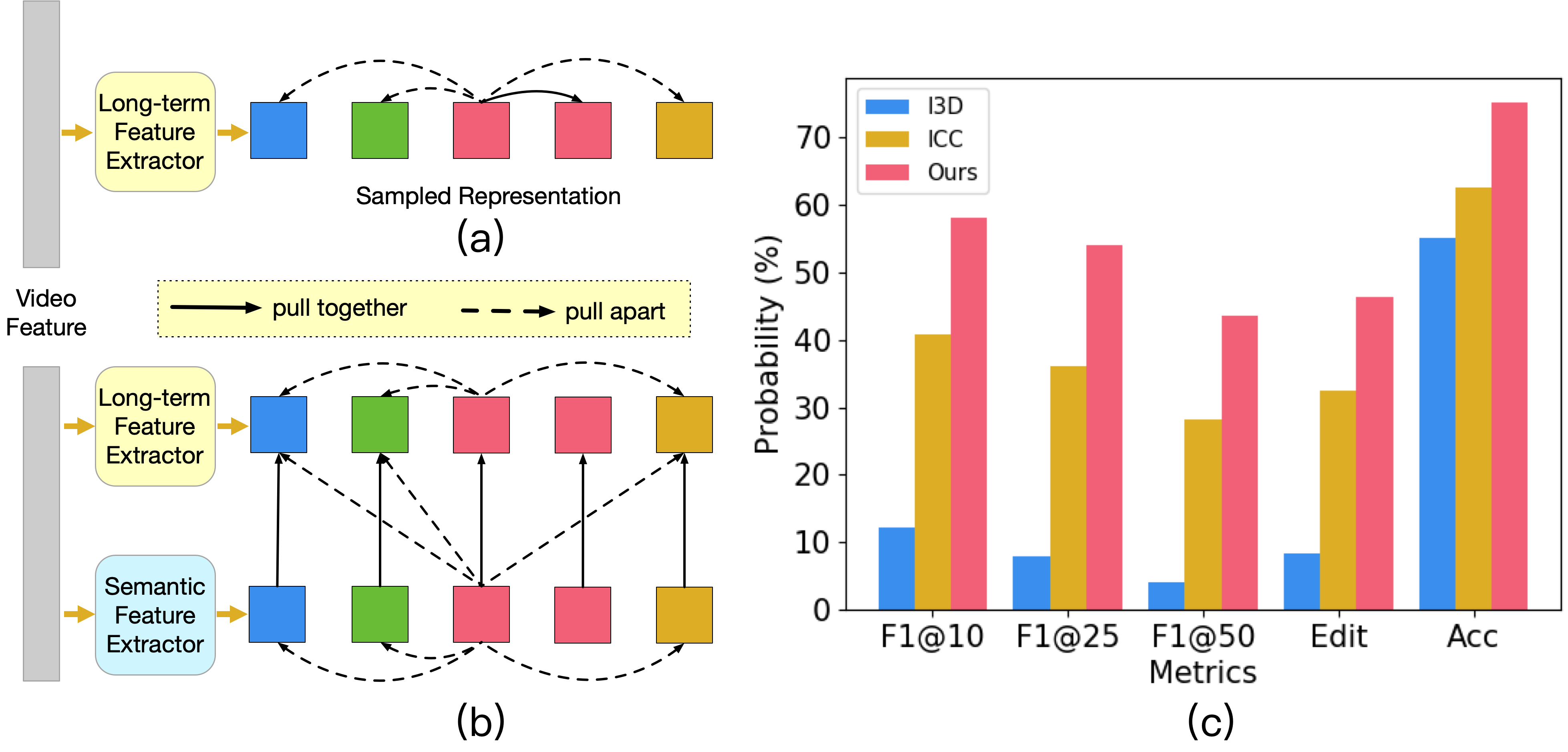
Figure 1: Comparisons of ICC [16] and our SMC for unsupervised representation learning. Based on the sampled representation encoded by a long-term feature extractor, ICC shown in (a) constructs positive (red boxes with the same label) and negative (boxes with different colours) pairs for contrastive learning. Our SMC shown in (b) takes advantage of the temporal and semantic information to fully explore intra- and inter-information variations where three types of negative pairs (pairwise boxes connected by dotted lines in the semantic and temporal branches, and between the two branches) are created. (c) shows the performance of our learned representation on the 50Salads dataset.

Recently, semi-supervised approaches [16, 17, 18] for this task have attracted increasing attention, with a small percentage of labelled videos in the training set. Iterative-Contrast-Classify (ICC) [16] is the first attempt to explore semi-supervised learning for human action segmentation, which consists of two steps, i.e., unsupervised representation learning based on contrastive learning [19, 20] (Fig. 1(a)) and supervised learning. Constructing both positive and negative sets for contrastive learning mainly depends on the clustering results (i.e., labels generated by clustering) of pre-trained input features. Empirical evidence has shown that the outcome of contrastive learning can be severely affected by clustering errors. Besides, only long-term temporal features are leveraged for similarity contrast, which would also limit the ability of representation learning. Another method for this topic is leveraging the correlation of actions between the labelled and unlabelled videos, and temporal continuity of actions [17]. However, their method only relies on action frequency prior in labelled data to build such correlations, rendering it inadequate for guiding the learning of complex unlabelled videos. Consequently, how to effectively explore the critical relations underlying the labelled and unlabelled videos is still an open and challenging problem.

In this paper, we propose a novel SMC-NCA framework for semi-supervised action segmentation. We first propose a novel Sematic-guided Multi-level Contrast (SMC) strategy to enhance frame-level representation learning by combining semantic and temporal information at the same time. Specifically, we introduce a long-term feature extractor and a semantic feature extractor to yield temporal and semantic information, respectively, as shown in Fig. 1(b). Semantic information emphasises action-specific characteristics in contrast to temporal information that encodes the dependencies between actions. Hence, we argue that leveraging the two types of information can help to facilitate contrastive learning. The two extractors are then jointly optimised by our SMC for fully exploring inter-information (between semantic and temporal information) and intra-information variations. Different from [16], our loss is built on triplet losses [21, 22, 23] where anchor, positive and negative representations need to be created. Therefore, we regard the semantic and temporal information as the anchor and positive representations to form positive pairs (i.e., pairwise boxes connected by solid lines in Fig. 1(b)) while explicitly constructing three kinds of negative pairs (e.g., pairwise boxes connected by dotted lines in the semantic branch) densely sampled from the anchor or negative representations. In particular, the generation of the negative pairs is determined by our proposed dynamic clustering scheme on the original input, encoded semantic and temporal features. In contrast, producing positive pairs relies on the inherent similarity between semantic and temporal information without knowing the clustering results.

Inspired by [16], we then iteratively perform supervised learning for action segmentation and unsupervised contrasting for representation updating. However, there still exist significant over-segmentation errors [24] when we use a small amount of labelled data for training the system. Thus, we further propose a Neighbourhood-Consistency-Aware (NCA) unit to explore the consistency between neighbourhoods (i.e., action segments) centered at different frames. Intuitively, feature distributions within the neighbourhoods of the same label should be spatially close. This NCA module can be combined with the SMC method to deal with the over-segmentation issue, particularly when we conduct learning with a small amount of labelled data.

Our main contributions are highlighted as follows:

• We propose a novel SMC-NCA framework for semi-supervised temporal action segmentation, where semantic and temporal information are jointly utilised to enhance representation learning.

• We propose a novel Semantic-guided Multi-level Contrast (SMC) scheme for unsupervised representation learning, allowing one to fully explore intra- and inter-information variations for learning discriminative frame-wise representations with the support of semantic information. This is achieved by constructing positive pairs and three distinct types of complementary negative pairs to facilitate contrastive learning.

• We propose a Neighbourhood-Consistency-Aware (NCA) unit to alleviate the over-segmentation problem in semi-supervised settings by utilising inter-neighbourhood consistency. This enables significant improvements of action segmentation in the case of a low number of labelled videos.

• Experimental results demonstrate that our proposed SMC scheme significantly improves the capability of frame-wise representation. Our SMC-NCA framework outperforms state-of-the-art methods across different settings of labelled data (5$\%$, 10$\%$, 40$\%$ and 100$\%$) on three challenging datasets and our mouse behaviour dataset.

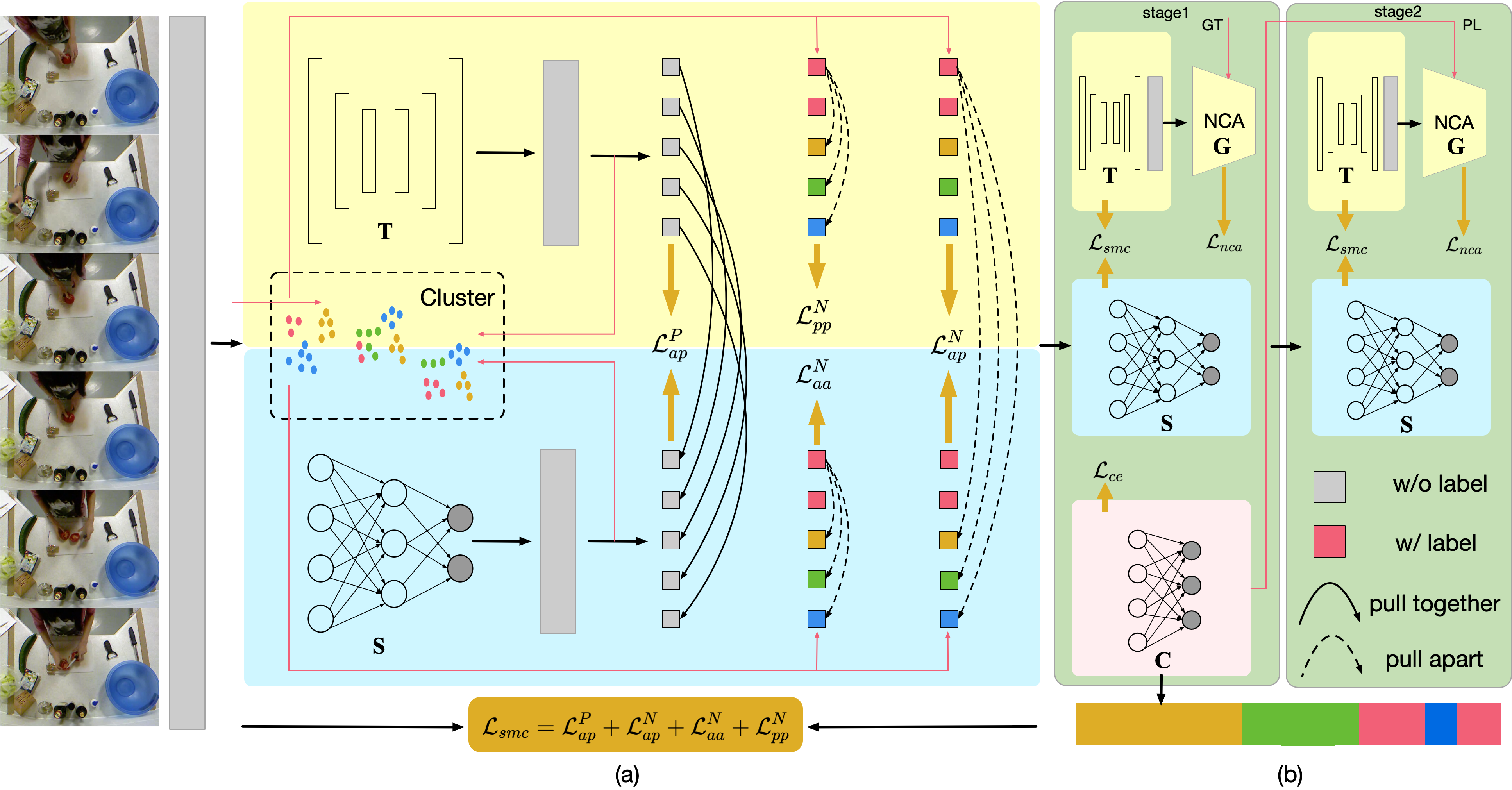
Figure 2: Our proposed semi-supervised learning framework for temporal action segmentation. (a) Unsupervised representation learning. The pre-trained I3D features are fed into the long-term feature extractor T and the semantic feature extractor S to generate temporal and high-level semantic representations, respectively. The representations are sampled, followed by performing Semantic-guided Multi-level Contrast. (b) Semi-supervised learning. In stage1, our Neighbourhood-Consistency-Aware unit G works closely with SMC, and the classification layer C can produce pseudo-labels (PL) used to guide the subsequent contrastive learning (stage2). $\mathcal{L}_{ap}^{N}$, $\mathcal{L}_{aa}^{N}$ and $\mathcal{L}_{pp}^{N}$ denote the negative losses of three negative pairs which are driven by the clustering results. $\mathcal{L}_{ap}^{P}$ represents the positive loss without relying on the clustering labels. $\mathcal{L}_{nca}$ is generated in the NCA module. Note that two models S and G are only used for training in order to facilitate learning and will not be used during the inference stage.

II Related Work

II-A Temporal Action Segmentation

Temporal action segmentation has been an increasingly popular trend in the domain of video understanding, which involves different levels of supervision. Fully-supervised methods require that each frame in the training videos be labelled. Earlier approaches have attempted to incorporate high-level temporal modelling over frame-wise classifiers. Kuehne et al. [25] utilised Fisher vectors of improved dense trajectories to represent video frames, and modelled each action with a Hidden Markov Model (HMM). Singh et al. [26] used a two-stream network to learn representations of short video chunks, which are then fed into a bi-directional LSTM to capture dependencies between different chunks. However, their approaches are computationally intensive due to sequential prediction. Most recent approaches employ TCN (temporal convolutional network) [6, 27, 28], GCN (graph convolution network) [29, 30] or Transformer [31] to model the long-range temporal dependencies in the videos. In spite of their promising performance, obtaining annotations on fine-grained actions for each frame is costly. Weakly-supervised methods mainly focus on transcript-level (with action order information) [9, 10, 11], set-level (without action order information) [12, 13, 14] and timestamp-level [15] supervisions to reduce the annotation effort. However, necessary supervision information is also needed for each video in the training set. Unsupervised approaches [32, 33, 34, 35] take advantages of clustering algorithms without any supervised signal per video, which still suffers from poor performance compared to other supervised settings.

II-B Unsupervised Contrastive Representation Learning

Recently, contrastive representation learning has been extensively used in different computer vision applications such as image representation learning [36, 19, 37, 38], video representation learning [39, 40, 41, 42, 43, 44, 20], time series representation learning [45, 46, 23] and face recognition [21, 47, 48, 49]. Among these approaches, contrastive loss[19, 36] and triplet loss [21, 23] are two popular loss functions to perform contrasting. The underlying idea behind the former is to pull together representations of augmented samples of the same image or video clips (i.e., positive pair) while pulling apart those of different instances (i.e., negative pair). The latter has the same goal but involves defining a triplet of (anchor, positive and negative pairs), where the positive pairs (i.e., anchor and positive representations) should be close and the negative pairs (i.e., anchor and negative representations) should be far apart. Our proposed framework is based on the triplet loss, which is the first attempt to explore complementary information between temporal and semantic information for semi-supervised temporal action segmentation.

III Proposed Method

The overall framework of our SMC-NCA is illustrated in Fig. 2. For unsupervised representation learning, given the input video features, a long-term feature extractor T and semantic feature extractor S are jointly adopted to extract temporal and semantic information. Our SMC is able to not only learn intra-information variation but also inter-information variation, where the temporal information describes the temporal dependencies between actions while semantic information highlights the action-specific characteristics. For semi-supervised learning, the models T, S and a linear classifier C are firstly integrated to perform supervised learning on a small number of labelled videos, followed by a new round of contrastive learning based on the pseudo-labels provided by C. An additional NCA unit (G) is designed in conjunction with contrastive learning to measure the spatial consistency between different neighbourhoods for the alleviation of over-segmentation errors. Following [16], we perform classification and contrastive learning in an iterative manner.

III-A Preliminaries on Contrastive Learning

Contrastive loss. InfoNCE loss [37, 19, 36] is usually used for optimisation in unsupervised representation learning. It is calculated on images or video clips with the common goal of encouraging instances of the same class to be approaching, and pushing the instances of different classes apart from each other in the embedding space. Following the formalism of [19, 16], we define a set of features $\mathcal{F}=\left\{\mathbf{f}_{i}|i\in\mathcal{I}\right\}$, which is represented as a matrix $\mathbf{X}$ ($\mathbf{X}[i]=\mathbf{f}_{i}$). $\mathcal{I}$ denotes the set of feature indices and each feature $\mathbf{f}_{i}$ has an unique class. Thus, given $\mathbf{X}[i]$, the positive set $\mathcal{P}_{i}\subset\mathcal{I}$ consisting of indices of features that have the same class as $\mathbf{X}[i]$, and the corresponding negative set $\mathcal{N}_{i}$, the contrastive loss for each $j\in\mathcal{P}_{i}$ is defined as:

$$\begin{split}\mathcal{L}_{cont}(i,j)=-\log\frac{e^{\operatorname{sim}\left(\mathbf{X}[i],\mathbf{X}[j]\right)/\tau}}{e^{\operatorname{sim}\left(\mathbf{X}[i],\mathbf{X}[j]\right)/\tau}+\sum\limits_{k\in\mathcal{N}_{i}}e^{\operatorname{sim}\left(\mathbf{X}[i],\mathbf{X}[k]\right)/\tau}}\end{split}$$ (1)

where $\operatorname{sim}(\mathbf{X}[i],\mathbf{X}[j])=\mathbf{X}[i]^{\top}\mathbf{X}[j]/\|\mathbf{X}[i]\|_{2}\|\mathbf{X}[j]\|_{2}$ is the inner product between two $\ell_{2}$ normalised vectors. $\tau>0$ is a temperature parameter.

Triplet loss. Unlike the contrastive loss, triplet loss [21, 23] requires to define a triplet $(\mathbf{X}[a],\mathbf{X}[p],\mathbf{X}[n])$ where $\mathbf{X}[a]$, $\mathbf{X}[p]$ and $\mathbf{X}[n]$ represent the anchor, positive and negative representations, respectively. This loss attracts positive pairs, $\mathbf{X}[a]$ (anchor) and $\mathbf{X}[p]$ (positive), while pushing away negative pairs, $\mathbf{X}[a]$ and $\mathbf{X}[n]$ (negative). Following [23], the triplet loss is formulated as:

$$\begin{split}\mathcal{L}_{trip}(a,p,n)=&-\log\Big{(}\sigma(\mathbf{X}[a]^{\top}\mathbf{X}[p])\Big{)}\\ &-\log\Big{(}\sigma(-\mathbf{X}[a]^{\top}\mathbf{X}[n])\Big{)}\end{split}$$ (2)

where $\sigma$ is the sigmoid function. The core of the triplet loss is to effectively generate the three representations.

III-B Problem Definition

A video sequence can be represented as $\textbf{V}\in\mathbb{R}^{T\times F}$ where $T$ is the total number of frames and $F$ represents the dimension of the pre-trained I3D features [50]. Each video frame $V[t]\in\mathbb{R}^{F}$ has a ground-truth action label $y[t]\in\{1,\ldots,A\}$ where $A$ denotes the number of the classes. We use an encoder-decoder model, i.e., C2F-TCN [28] as our base segmentation network T. Therefore, given the input video features V, we aim to learn the unsupervised model $\left(\textbf{T}:\textbf{S}\right)$ by our Semantic-guided Multi-level Contrast on the dataset $\mathcal{D}=\mathcal{D}_{U}\cup\mathcal{D}_{L}$ ($\mathcal{D}_{U}$ and $\mathcal{D}_{L}$ denote the unlabelled and labelled videos, respectively) where T and S are the temporal and semantic models, respectively. Subsequently, the Neighbourhood-Consistency-Aware module G and a linear mapping layer C are added to form semi-supervised model $\left(\textbf{T}:\textbf{S}:\textbf{G}:\textbf{C}\right)$ which is trained on a small subset of labelled training videos $\mathcal{D}_{L}$. We follow the standard operation of [16], where we first use the same down-sampling strategy to obtain coarser features (i.e., input) of temporal dimension $T$. In the inference, the final predictions are up-sampled to the original full resolution with temporal dimension $T_{ori}$ to compare with the original ground truth.

III-C Semantic-guided Multi-level Contrast

As mentioned earlier, we propose to leverage both temporal and semantic information to our proposed SMC module, where the former describes long-range temporal dependencies in long videos while the latter encodes high-level features at each action/frame. In the SMC module, inter- and intra-information variations are jointly learned to enhance the discriminative power of the temporal model.

Temporal and semantic information generation. To encode the correlation between actions, we adopt the C2F-TCN [16] model to produce a multi-resolution representation (denoted as $\textbf{X}=\textbf{T}(\textbf{V})\in\mathbb{R}^{N\times T\times D}$, where $N$ is the minibatch size during training, $D$ represents the feature dimension of the generated representation) with temporal information used for unsupervised contrastive learning. In the meanwhile, we employ the multilayer perceptron (MLP) as a semantic feature extractor on the same input video features V to generate a new representation (denoted as $\textbf{H}=\textbf{S}(\textbf{V})\in\mathbb{R}^{N\times T\times D}$) with high-level semantic information. A MLP offers simplicity and efficiency (we also tested other extractors, such as deeper MLPs and 1D CNNs, see Tab. IV). The model S can be formulated as:

$$\begin{split}\mathbf{V}^{(l+1)}&=\sigma\left(\mathbf{V}^{(l)}\mathbf{W}^{(l)}+b^{(l)}\right)\\ \mathbf{H}&=\mathbf{V}^{(l+1)}\mathbf{W}^{(l+1)}+b^{(l+1)}\end{split}$$ (3)

where $\mathbf{V}^{(l)}\in\mathbb{R}^{N\times T\times D^{l}}$ denotes the input hidden representation from the previous layer (with $\mathbf{V}^{(0)}=\mathbf{V}$) and $\mathbf{W}^{(l)}\in\mathbb{R}^{D^{l}\times D^{l+1}}$ and $b^{(l)}$ are trainable parameters. $\sigma$ is an activation function.

Inter-information variation learning. In our contrastive learning framework, we fully explore the complementary information between the temporal and semantic information, based on the encoded representation X and H. To achieve this, we firstly learn the similarity and dissimilarity between the two different representations. Specifically, we firstly sample a fixed number of frames from each training video to form a new temporal representation $\textbf{X}_{s}\in\mathbb{R}^{N\times T_{s}\times D}$ and semantic representation $\textbf{H}_{s}\in\mathbb{R}^{N\times T_{s}\times D}$ using the same sampling strategy reported in [16], where $T_{s}$ is the number of the sampled frames from each video. It is too computationally expensive to measure each frame of every video in a mini-batch. The sampled frames for each video are then combined together by concatenation operation on the dimension $T$ to form $\textbf{X}_{s}\in\mathbb{R}^{N\cdot T_{s}\times D}$ and $\textbf{H}_{s}\in\mathbb{R}^{N\cdot T_{s}\times D}$.

The features of pairwise video frames with the same index in $\textbf{X}_{s}$ and $\textbf{H}_{s}$ describe the same action (boxes connected by solid lines in Fig. 1(b)). In this way, we identify $\textbf{X}_{s}$ and $\textbf{H}_{s}$ as positive and anchor representations respectively, and our goal is to pull them (i.e., positive pairs) together. Inspired by [23], given $\textbf{X}_{s}$ and $\textbf{H}_{s}$, we formalise the objective function of the inter-information similarity learning as:

$$\begin{split}\Psi_{ap}^{P}&=-\Big{[}\log\Big{(}\sigma(\mathbf{H}_{s}^{\top}\mathbf{X}_{s}/\xi)\Big{)}\Big{]}\odot\mathbf{I}\\ &=\begin{bmatrix}\Psi_{ap}^{P}[1,1]&&\\ &\ddots&\\ &&\Psi_{ap}^{P}[N\cdot T_{s},N\cdot T_{s}]\\ \end{bmatrix}\end{split}$$ (4)

where $\odot$ represents element-wise product. $\mathbf{I}\in\mathbb{R}^{N\cdot T_{s}\times N\cdot T_{s}}$ represents the identity matrix used to select pairwise frames with the same index, and $0<\xi<1$ is a scale factor to adjust the correlation between vectors. $\Psi_{ap}^{P}[,]$ is the element of matrix $\Psi_{ap}^{P}$.

The advantages of optimising this function are two-folds. Firstly, we consider the temporal and semantic information simultaneously, which is beneficial to improving the ability of representation learning. Secondly, learning of positive pairs (anchor and positive representations) is not dependent on the coarse clustering results, compared to ICC that generates related contrastive instances based on clustering results. In contrast, $\Psi_{ap}^{P}$ performs contrastive learning with the guide of the potential similarity between frame-wise temporal and semantic representations. We then compute the overall loss $\mathcal{L}_{ap}^{P}$ between positive pairs below:

$$\begin{split}\mathcal{L}_{ap}^{P}=\frac{1}{N\cdot T_{s}}\sum_{i=1}^{N\cdot T_{s}}(\Psi_{ap}^{P}[i,i])\end{split}$$ (5)

Operations such as random selection [23] or shuffling [39] are usually used to generate negative pairs in the existing works for unsupervised contrastive learning [51, 43, 23, 48]. However, these strategies are usually used for short temporal sequences and they cannot be directly applied to temporal action segmentation due to the complex and various actions in long videos. Here, we further exploit two types of complementary information i.e., temporal and semantic representations to create negative pairs for uncovering their differences. Different from learning inter-information similarity without any auxiliary label information shown in Eq. (4), the construction of negative pairs relies on the results of K-means clustering. Specifically, we can choose pairwise frames with different clustering labels, followed by contrasting these frames. For the $t$-frame in $\textbf{V}_{s}$, the clustering label generated by K-means can be denoted as $l_{in}[t]$. We can further obtain a matrix, i.e., $\textbf{M}_{in}$, which consists of the similarity between any two frames. Regarding the matrix $\textbf{M}_{in}$, we have:

$$\begin{split}\textbf{M}_{in}[i,j]=\begin{cases}1\text{, }l_{in}[i]=l_{in}[j],\forall i,j\in\left\{1,2,\dots,N\cdot T_{s}\right\}\\ 0\text{, }other\end{cases}\end{split}$$ (6)

The clustering results on the standard input features $\textbf{V}_{s}$ cannot be updated, which may lead to accumulation errors caused by incorrect negative pairs. To reduce these errors, we perform the clustering on the sampled input $\textbf{V}_{s}$, temporal $\textbf{X}_{s}$ and semantic $\textbf{H}_{s}$ features simultaneously for dynamic selection of potential negative pairs. Hence, we obtain $\textbf{M}_{te}$ and $\textbf{M}_{se}$ for $\textbf{X}_{s}$ and $\textbf{H}_{s}$, respectively. By combining the three matrices, we generate a matrix $\textbf{M}\in\mathbb{R}^{N\cdot T_{s}\times N\cdot T_{s}}$ that is used to dynamically guide the dissimilarity learning on the negative pairs, defined as:

$$\begin{split}\textbf{M}=(1-\textbf{M}_{in})\odot(1-\textbf{M}_{te})\odot(1-\textbf{M}_{se})\end{split}$$ (7)

where each element $\textbf{M}[i,j]\in\left\{0,1\right\}$ indicates whether or not the $i$-th and $j$-th frames share the same clustering label.

Afterwards, we can construct a set of dense negative pairs for each frame based on M, and negative pairs must be separate. Hence, similar to Eq. (4), the function $\Psi_{ap}^{N}$ to be minimised with the corresponding loss $\mathcal{L}_{ap}^{N}$ is expressed as:

$$\begin{split}\Psi_{ap}^{N}&=-\Big{[}\log\Big{(}\sigma(-\mathbf{H}_{s}^{\top}\mathbf{X}_{s}/\xi)\Big{)}\Big{]}\odot\mathbf{M}\end{split}$$ (8)

$$\begin{split}\mathcal{L}_{ap}^{N}=\frac{1}{N_{ap}}\sum_{i=1}^{N\cdot T_{s}}\sum_{j=1}^{N\cdot T_{s}}(\Psi_{ap}^{N}[i,j])\end{split}$$ (9)

where $N_{ap}=\sum_{i=1}^{N\cdot T_{s}}\sum_{j=1}^{N\cdot T_{s}}(\mathbf{M}[i,j])$ denotes the number of all the negative pairs.

Intra-information variation learning. $\mathcal{L}_{ap}^{P}$ and $\mathcal{L}_{ap}^{N}$ defined in Eqs. (5) and (9) encourage the temporal model to focus on the inter-information variations. Although they implicitly learn the dissimilarity between frames with the semantic or temporal representation, the discriminability of the learned representations is still weak (this can be further verified in Section IV-C1). Therefore, we further explore the intra-information variations, including the dissimilarities within the semantic and temporal representations. For each frame of semantic representations (anchor), we choose all the other frames with different clustering labels to form a set of dense intra-information negative pairs. The overall loss for measuring the dissimilarity between negative pairs with anchor representation $\mathbf{H}_{s}$ can be computed as:

$$\begin{split}\Psi_{aa}^{N}&=-\Big{[}\log\Big{(}\sigma(-\mathbf{H}_{s}^{\top}\mathbf{H}_{s}/\xi)\Big{)}\Big{]}\odot\mathbf{M}\end{split}$$ (10)

$$\begin{split}\mathcal{L}_{aa}^{N}=\frac{1}{N_{ap}}\sum_{i=1}^{N\cdot T_{s}}\sum_{j=1}^{N\cdot T_{s}}(\Psi_{aa}^{N}[i,j])\end{split}$$ (11)

Additionally, we consider the dissimilarity between frames of temporal representations $\mathbf{X}_{s}$ (positive), and the corresponding loss is defined as follows:

$$\begin{split}\Psi_{pp}^{N}&=-\Big{[}\log\Big{(}\sigma(-\mathbf{X}_{s}^{\top}\mathbf{X}_{s}/\xi)\Big{)}\Big{]}\odot\mathbf{M}\end{split}$$ (12)

$$\begin{split}\mathcal{L}_{pp}^{N}=\frac{1}{N_{ap}}\sum_{i=1}^{N\cdot T_{s}}\sum_{j=1}^{N\cdot T_{s}}(\Psi_{pp}^{N}[i,j])\end{split}$$ (13)

Finally, integrating inter-information losses (i.e., Eqs. (5) and (9)) with the intra-information losses in Eqs. (11) and (13), our proposed sematic-guided multi-level contrast loss is formulated as:

$$\begin{split}\mathcal{L}_{smc}=\mathcal{L}_{ap}^{P}+\mathcal{L}_{ap}^{N}+\mathcal{L}_{aa}^{N}+\mathcal{L}_{pp}^{N}\end{split}$$ (14)

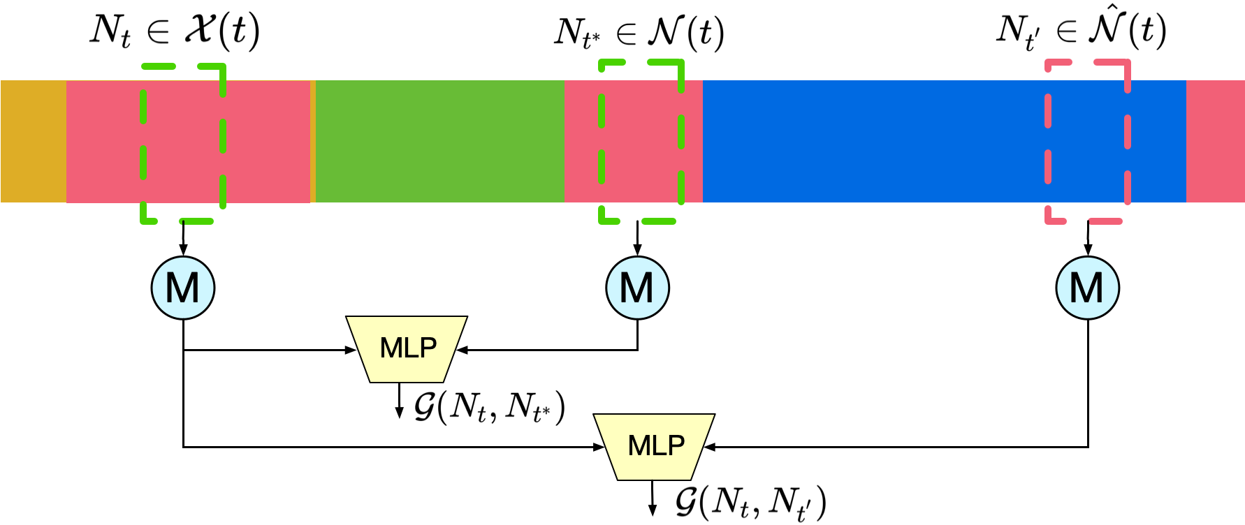
Figure 3: Illustration of the proposed Neighbourhood-Consistency-Aware Unit. We randomly sample a frame $t$, and its neighbourhood is $N_{t}$ (left green dashed box). Then we can use frame $t^{*}$ with the same label to form the neighbourhood $N_{t^{*}}$. The two neighbourhoods are fed into the max-pooling layer to encode their feature distributions, followed by predicting the probability of having similar feature distributions by the MLP model. The same operation is applied to $N_{t}$ and $N_{t^{{}^{\prime}}}$ centered at frames $t$ and $t^{{}^{\prime}}$ with different labels.

III-D Neighbourhood-Consistency-Aware Unit

After having trained the unsupervised model $\left(\textbf{T}:\textbf{S}\right)$ by our SMC module, we perform semi-supervised learning for frame-wise classification of temporal actions, as shown in Fig. 2(b). However, over-segmentation [24], which is a critical problem in action segmentation, accompanies over-fitting. Over-segmentation refers to the error type where a video is excessively divided into subsegments, causing erratic action class predictions. In order to alleviate this issue in our semi-supervised setting, we introduce a Neighbourhood-Consistency-Aware module shown in Fig. 3 to ensure spatial consistency between action segments. The intuition behind this is that feature distributions within the neighbourhoods of the same label should be spatially close. We further discuss the NCA module below.

After having trained the unsupervised model $\left(\textbf{T}:\textbf{S}\right)$ by our SMC module, we perform semi-supervised learning for frame-wise classification of temporal actions, as shown in Fig. 2(b). However, over-segmentation [24], which is a critical problem in action segmentation, accompanies over-fitting. In order to alleviate this issue in our semi-supervised setting, we introduce a Neighbourhood-Consistency-Aware module shown in Fig. 3 to ensure spatial consistency between action segments. We further discuss the NCA module below.

At the first stage shown in Fig. 2(b), given the temporal representation X of a video with ground truth labels $l$ in the batch, we randomly sample $K$ frames and construct $K$ neighbourhoods centered at these frames. For each frame, we then select $M$ frames having the same label and $M$ frames with different labels, respectively. Formally, we define the sets of neighbourhoods as:

$$\begin{split}\mathcal{X}(t)&=\left\{N_{t}=\mathbf{X}[t-\frac{W}{2},t+\frac{W}{2}]|t\in\mathcal{Z}(t)\right\}\\ \mathcal{N}(t)&=\left\{N_{t^{*}}=\mathbf{X}[t^{*}-\frac{W}{2},t^{*}+\frac{W}{2}]|t^{*}\in\mathcal{P}(t)\right\}\\ \hat{\mathcal{N}}(t)&=\left\{N_{t^{{}^{\prime}}}=\mathbf{X}[t^{{}^{\prime}}-\frac{W}{2},t^{{}^{\prime}}+\frac{W}{2}]|t^{{}^{\prime}}\in\hat{\mathcal{P}}(t)\right\}\end{split}$$ (15)

where $W$ is the length of an action segment. $\mathcal{N}(t)$ represents a set of $M$ segments, where each segment consisting of $W$ frames is centered at one frame from a group of $M$ frames. The $M$ frames are randomly sampled from the video frames that have the same label as the frame $t$. For $\hat{\mathcal{N}}(t)$, $M$ frames are randomly sampled from the video frames that have different labels from frame $t$. $\mathcal{Z}(t)=\left\{t_{i}|1\leq i\leq K\right\}$ represents the indices of the sampled $K$ frames. $\mathcal{P}(t)=\left\{t^{*}|l[t^{*}]=l[t],\frac{W}{2}\leq t^{*}\leq T-\frac{W}{2}\right\}$ and $\hat{\mathcal{P}}(t)=\left\{t^{*}|l[t^{*}]\neq l[t],\frac{W}{2}\leq t^{*}\leq T-\frac{W}{2}\right\}$ denotes the indices of the frames with the same and different labels corresponding to the $t$-th frame, respectively.

Algorithm 1 The learning process of our SMC-NCA framework.

0:  Input features $\mathbf{V}$, temporal representation $\mathbf{X}$ and semantic representation $\mathbf{H}$.

1:  Generate sampled $\mathbf{V_{s}}$, $\mathbf{X_{s}}$ and $\mathbf{H_{s}}$

2:  for  epoch $e\leftarrow 1$ to E1  do

3:     $\mathcal{L}_{ap}^{P}\leftarrow-Sum\Big{(}\Big{[}\log\Big{(}\sigma(\mathbf{H}_{s}^{\top}\mathbf{X}_{s}/\xi)\Big{)}\Big{]}\odot\mathbf{I}\Big{)}/Sum(\mathbf{I})$

4:     $\textbf{M}\leftarrow Cluster(\mathbf{V}_{s},\mathbf{X}_{s},\mathbf{H}_{s})$

5:     $\mathcal{L}_{ap}^{N}\leftarrow-Sum\Big{(}\Big{[}\log\Big{(}\sigma(-\mathbf{H}_{s}^{\top}\mathbf{X}_{s}/\xi)\Big{)}\Big{]}\odot\mathbf{M}\Big{)}/Sum(\mathbf{M})$

6:     $\mathcal{L}_{aa}^{N}\leftarrow-Sum\Big{(}\Big{[}\log\Big{(}\sigma(-\mathbf{H}_{s}^{\top}\mathbf{H}_{s}/\xi)\Big{)}\Big{]}\odot\mathbf{M}\Big{)}/Sum(\mathbf{M})$

7:     $\mathcal{L}_{pp}^{N}\leftarrow-Sum\Big{(}\Big{[}\log\Big{(}\sigma(-\mathbf{X}_{s}^{\top}\mathbf{X}_{s}/\xi)\Big{)}\Big{]}\odot\mathbf{M}\Big{)}/Sum(\mathbf{M})$

8:     $\mathcal{L}_{smc}\leftarrow\mathcal{L}_{ap}^{P}+\mathcal{L}_{ap}^{N}+\mathcal{L}_{aa}^{N}+\mathcal{L}_{pp}^{N}$ (on $\mathcal{D}$)

9:     Minimize $\mathcal{L}_{smc}$ and update models $\mathbf{T}$ and $\mathbf{S}$

10:  end for

11:  Obtain the best model evaluated by the linear classifier

12:  for  iter $i\leftarrow 1$ to $I$ do

13:     for  epoch $e\leftarrow 1$ to E2  do

14:        $\textbf{M}\leftarrow$ GT

15:        $\mathcal{L}_{smc}\leftarrow\mathcal{L}_{ap}^{P}+\mathcal{L}_{ap}^{N}+\mathcal{L}_{aa}^{N}+\mathcal{L}_{pp}^{N}$ (on $\mathcal{D}_{L}$)

16:        Sample $t\in\mathcal{Z}(t)=\left\{t_{i}|1\leq i\leq K\right\}$

17:        $\mathcal{L}_{nca}\leftarrow NCA(t)$

18:        $\mathcal{L}\leftarrow\small\mathcal{L}_{smc}+\mathcal{L}_{nca}+\mathcal{L}_{ce}$

19:        Minimize $\mathcal{L}$ and update models $\mathbf{T}$, $\mathbf{S}$, $\mathbf{G}$ and $\mathbf{C}$

20:     end for

21:     for  epoch $e\leftarrow$ 1 to E3 do

22:        PL $\leftarrow\mathbf{C}(\mathcal{D}_{U})$

23:        $\textbf{M}\leftarrow$ PL $\cup$ GT

24:        $\mathcal{L}\leftarrow\small\mathcal{L}_{smc}+\mathcal{L}_{nca}$ (on $\mathcal{D}$)

25:        Minimize $\mathcal{L}$ and update models $\mathbf{T}$, $\mathbf{S}$ and $\mathbf{G}$ on $\mathcal{D}$

26:     end for

27:  end for

Our NCA module aims at detecting the inter-neighbourhood consistency, where $N_{t}$ and $N_{t^{*}}$ tend to have similar feature distributions, whereas the distributions of $N_{t}$ and $N_{t^{{}^{\prime}}}$ may be different. We define the problem of consistency detection as minimisation practice:

$$\begin{split}\begin{aligned} \mathcal{L}_{nca}=&-\mathbb{E}_{N_{t}\sim\mathcal{X}(t)}\Big{[}\mathbb{E}_{N_{t^{*}}\sim\mathcal{N}(t)}\left[\log\mathcal{G}\left(N_{t},N_{t^{*}}\right)\right]\\ &+\mathbb{E}_{N_{t^{{}^{\prime}}}\sim\hat{\mathcal{N}}(t)}\left[\log\left(1-\mathcal{G}\left(N_{t},N_{t^{{}^{\prime}}}\right)\right)\right]\Big{]}\end{aligned}\end{split}$$ (16)

where $\mathbb{E}$ represents the expectation. $\mathcal{G}\left(N_{t},N_{t^{*}}\right)$ results in the probability of the neighbourhoods having similar feature distributions, formulated as follows:

$$\begin{split}\begin{aligned} \mathcal{G}(N_{t},N_{t^{*}})=\textbf{G}([max(N_{t});max(N_{t^{*}})])\end{aligned}\end{split}$$ (17)

where G is a MLP block similar to S in Eq. (3). $[;]$ represents the concatenation operation. $max(\cdot)$ means max-pooling used to aggregating temporal features [52, 53].

The loss function can be approximated as:

$$\begin{split}\begin{aligned} \mathcal{L}_{nca}=&-\frac{1}{K\times M}\sum_{i=1}^{K}\sum_{j=1}^{M}\Big{[}\log\mathcal{G}(N_{t}^{i},N_{t^{\ast}}^{j})+\\ &\log(1-\mathcal{G}(N_{t}^{i},N_{t^{{}^{\prime}}}^{j}))\Big{]}\end{aligned}\end{split}$$ (18)

At the second stage, the ground truth labels (GT) are combined with the pseudo labels (PL) generated by C at the first stage to guide the learning of G, T and S for updating representations. Our proposed SMC-NCA framework is summarised in Algorithm 1.

TABLE I: Training hyperparameters learning rate (LR), weight-decay (WD), epochs (Eps.) and Batch Size (BS) over different datasets for unsupervised and semi-supervised learning.

Model	Breakfast	50Salads	GTEA	PDMB
	LR  WD  Eps.  BS	LR  WD  Eps.  BS	LR  WD  Eps.  Bs	LR  WD  Eps.  Bs
(T: S)	le-3 3e-3  100  50	1e-3  1e-3  100 5	1e-3 3e-4  100  4	1e-3 3e-4  100  4
C	le-2 3e-3  200  50	1e-2  1e-3  400 5	1e-2 3e-4  400  4	1e-2 3e-4  400  4
(T:G:S)	le-5 3e-3  200  50	1e-5  1e-3  400 5	1e-5 3e-4  400  4	1e-5 3e-4  400  4

TABLE II: Component-wise analysis of the unsupervised representation learning framework with a linear classifier.

Method	50Salads	GTEA
	F1@{10, 25, 50}   Edit   Acc	F1@{10, 25, 50}   Edit   Acc
$\mathcal{L}_{ap}^{P}$($\textbf{M}_{in}$)+$\mathcal{L}_{aa}^{N}$	36.8  31.1 22.6  29.8  57.1	73.1  66.3 48.5  65.5  70.2
$\mathcal{L}_{ap}^{P}$(I)+$\mathcal{L}_{aa}^{N}$	51.9  46.8 38.2  39.7  72.4	75.8  71.1 53.0  68.0  73.8
$\mathcal{L}_{ap}^{P}$($\textbf{M}_{in}$)+$\mathcal{L}_{ap}^{N}$	39.1  33.8 25.2  31.8  56.4	69.8  63.7 48.3  64.3  68.8
$\mathcal{L}_{ap}^{P}$(I)+$\mathcal{L}_{ap}^{N}$	40.7  35.6 26.4  30.9  64.8	73.0  67.6 50.0  66.1  70.8
Constructing positive pairs by $\textbf{M}_{in}$ (rely on the clustering results) or $I$ (without relying on the clustering)
$\mathcal{L}_{ap}^{P}$ + $\mathcal{L}_{aa}^{N}$	51.9  46.8 38.2  39.7  72.4	75.8  71.1 53.0  68.0  73.8
$\mathcal{L}_{ap}^{P}$ + $\mathcal{L}_{ap}^{N}$	40.7  35.6 26.4  30.9  64.8	73.0  67.6 50.0  66.1  70.8
$\mathcal{L}_{ap}^{P}$ + $\mathcal{L}_{aa}^{N}$ + $\mathcal{L}_{ap}^{N}$	55.2  50.1 42.0  44.0  73.1	76.2  71.8 55.7  67.9  75.0
$\mathcal{L}_{ap}^{P}$ + $\mathcal{L}_{aa}^{N}$ + $\mathcal{L}_{ap}^{N}$ + $\mathcal{L}_{pp}^{N}$	56.5  52.1 42.8  45.4  74.3	77.4  71.2 56.1  69.0  75.7
Comparing different negative pairs
w/o dynamic clustering	56.5  52.1 42.8  45.4  74.3	77.4  71.2 56.1  69.0  75.7
w/ dynamic clustering	58.1  54.0 43.5  46.3  75.1	78.9  74.3 59.2  73.0  76.2
Dynamic clustering facilitates contrastive learning

TABLE III: Ablation study on the Breakfast dataset.

Method	Breakfast
	F1@{10, 25, 50}   Edit   Acc
$\mathcal{L}_{ap}^{P}$ + $\mathcal{L}_{aa}^{N}$	57.4  52.6 39.0  51.0  70.3
$\mathcal{L}_{ap}^{P}$ + $\mathcal{L}_{ap}^{N}$	56.3  51.2 38.4  50.3  69.1
$\mathcal{L}_{ap}^{P}$ + $\mathcal{L}_{aa}^{N}$ + $\mathcal{L}_{ap}^{N}$	58.2  54.1 41.0  52.1  71.7
$\mathcal{L}_{ap}^{P}$ + $\mathcal{L}_{aa}^{N}$ + $\mathcal{L}_{ap}^{N}$ + $\mathcal{L}_{pp}^{N}$	59.0  54.0 41.9  52.2  71.9
w/o dynamic clustering	59.0  54.0 41.9  52.2  71.9
w/ dynamic clustering	59.7  55.4 42.8  52.7  72.1

TABLE IV: Comparing semantic feature extractors on the 50Salads dataset.

Method	F1@{10, 25, 50}	Edit	Acc
MLP (1 layer)	58.1 54.0 43.5	46.3	75.1
MLP (3 layers)	45.4 41.0 32.5	37.3	61.9
MLP (5 layers)	39.4 34.6 25.1	32.3	57.6
Conv1d (1 layers)	55.1 50.0 41.0	44.1	72.0
Conv1d (3 layers)	42.7 38.6 28.1	34.6	59.3
Conv1d (5 layers)	37.9 32.5 22.9	31.4	54.1

IV Experiments

IV-A Datasets and Evaluation

Public Action Segmentation Datasets. We evaluate the proposed method on three challenging datasets: 50Salads [54] (50 videos, 19 actions), GTEA [55] (28 videos, 11 actions), and Breakfast Actions [56] (1712 videos, 10 complex activities, 48 actions). Following [16], we use the standard train-test splits for each dataset.

Mouse Social Behaviour Dataset. Based on the dataset from our previous works [57, 58], we introduce a new Parkinson’s Disease Mouse Behaviour (PDMB) dataset consisting of three groups of normal mice and three groups of mice with Parkinson’s Disease. It provides a valuable resource for the research community to investigate the behavioural patterns and characteristics associated with Parkinson’s Disease. More details can be found in Supplementary A.

Evaluation. We follow the evaluation protocol used in ICC [16] for both unsupervised and semi-supervised settings. In specific, for the public datasets, we use the same evaluation metrics taken for fully-supervised temporal action segmentation, including frame-wise accuracy (Acc), segmental edit distance (Edit), and segmental F1 score at overlapping thresholds 10$\%$, 25$\%$, and 50$\%$ (denoted as F1@{10, 25, 50}) [6]. The overlapping ratio is the intersection over union (IoU) ratio between the predicted and ground-truth action segments. We conduct cross-validation using the standard splits [16], and report the average. We evaluate the representation generated in unsupervised learning by training a linear classifier to classify frame-wise action labels. In the semi-supervised setting, we also report the average of 5 different selections to reduce the randomness brought by the training subset selection. For our PDMB dataset, we also use similar evaluation metrics and define 2 splits for cross-validation.

IV-B Implementation Details.

All our experiments are performed on Nvidia Tesla P100 GPUs with 16GB memory. The parameters are optimised by the Adam algorithm. Learning Rate (LR), Weight Decay (WD), Epochs (Eps), and Batch Size (BS) used for our unsupervised and semi-supervised setups can be found in Tab. I. Similar to [16], the number of iterations is set to 4. In the beginning of unsupervised representation learning, $\xi$ is set to 1 for 50salads, GTEA and our PDMB dataset, and 0.1 for the large dataset Breakfast. In the NCA module, the length of a neighbourhood $W$, the number of the selected frames $K$, and the number of frames $M$ with the same label for each selected frame is set to 8, 1 and 10, respectively. The source code will be published after the paper has been accepted.

IV-C Ablation Studies

IV-C1 Evaluation of Representation Learning

Effect of positive pairs construction. As defined in Eq. (4), we construct the positive pairs based on the inherent similarity between frame-wise representations with temporal and semantic information rather than matrix, e.g., $\textbf{M}_{in}$ from the clustering outcomes. Tab. II (Top) shows the impact of positive pair construction for the inter-information similarity learning on two public datasets (i.e., 50Salads and GTEA datasets). We replace I in Eq. (4) with $\textbf{M}_{in}$ to generate dense positive pairs, and the corresponding loss $\mathcal{L}_{ap}^{P}$($\textbf{M}_{in}$) is combined with $\mathcal{L}_{aa}^{N}$ and $\mathcal{L}_{ap}^{N}$ respectively for representation learning. As shown in Tab. II (Top), we experience a significant decrease in performance using the contrastive learning guided by $\textbf{M}_{in}$, especially on the 50Salads dataset. This is likely caused by the fact that such design results in more clustering errors which affect the inter-information similarity learning.

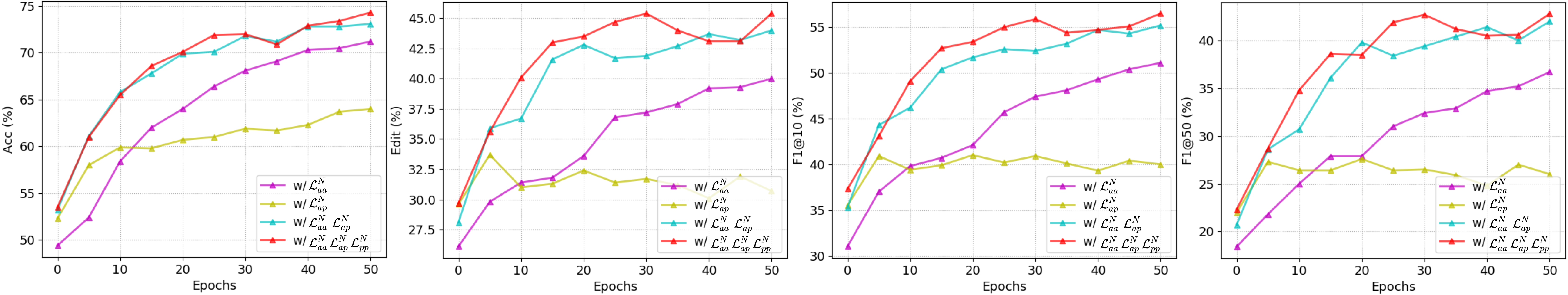
Figure 4: Performance of unsupervised representation learning using different loss functions during training on 50Salads.

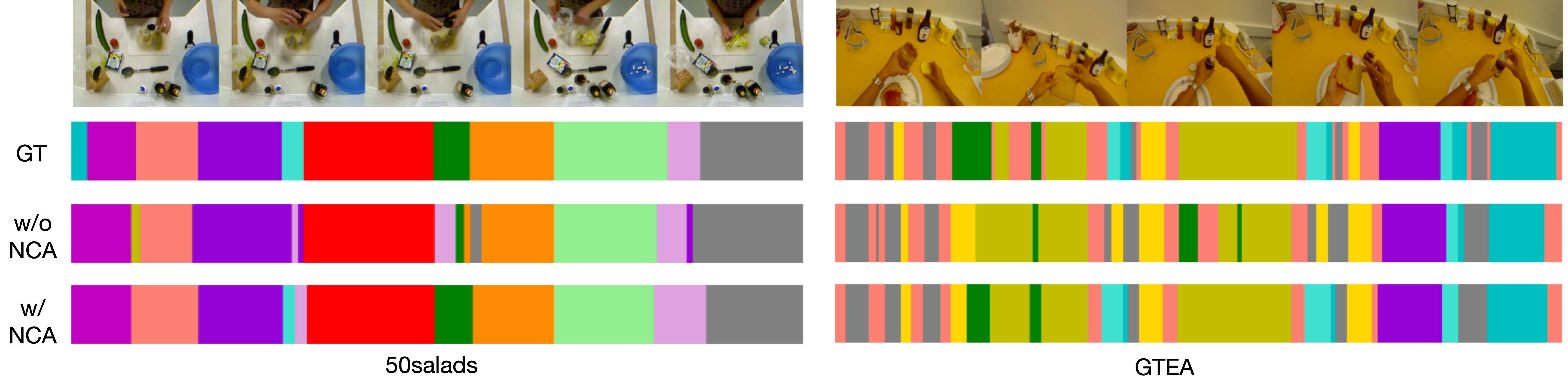
Figure 5: Qualitative results on the 50Salads and GTEA (5$\%$) datasets show the effects of our NCA module.

TABLE V: Comparing our proposed semi-supervised approach with the supervised learning approach using the same labelled data on the 3 benchmark datasets.

$\%D_{L}$	Method	50salads	GTEA	Breakfast
		F1@{10, 25, 50}  Edit  Acc	F1@{10, 25, 50}  Edit  Acc	F1@{10, 25, 50}  Edit  Acc
5	Supervised	30.5 25.4 17.3 26.3 43.1	64.9 57.5 40.8 59.2 59.7	15.7 11.8    5.9 19.8 26.0
	Semi-Super	57.0 53.1 42.1 48.9 68.9	81.9 79.3 64.0 77.9 73.9	62.7 57.0 41.6 60.2 68.9
	Gain	26.5 27.7 24.8 22.6 25.8	17.0 21.8 23.2 18.7 14.2	47.0 45.2 35.7 40.4 42.9
10	Supervised	45.1 38.3 26.4 38.2 54.8	66.2 61.7 45.2 62.5 60.6	35.1 30.6 19.5 36.3 40.3
	Semi-Super	70.3 66.3 54.7 61.3 73.6	87.7 84.2 71.7 83.3 77.5	64.8 60.2 45.0 63.4 69.7
	Gain	25.2 28.0 28.3 23.1 18.8	21.5 22.5 26.5 20.8 16.9	29.7 29.6 25.5 27.1 29.4
100	Supervised	75.8 73.1 62.3 68.8 79.4	90.1 87.8 74.9 86.7 79.5	69.4 65.9 55.1 66.5 73.4
	Semi-Super	86.9 84.8 78.9 80.7 87.0	92.7 91.0 81.5 88.3 82.6	73.8 69.7 56.8 70.9 76.4
	Gain	11.1 11.7 16.6 11.9   7.6	2.6   3.2   6.6   1.6   3.1	4.4   3.8   1.7   4.4   3.0

Effect of negative pairs construction. Tab. II (Middle) illustrates the results of the combinations of loss functions. In our SMC framework, we construct three types of dense negative pairs from the representations with temporal, semantic information and their combinations, respectively (the corresponding losses can be annotated as $\mathcal{L}_{pp}^{N}$, $\mathcal{L}_{aa}^{N}$ and $\mathcal{L}_{ap}^{N}$). As shown in Tab. II (Middle), compared with $\mathcal{L}_{ap}^{N}$, $\mathcal{L}_{aa}^{N}$ achieves better F1 and Edit scores and accuracy, with improvements of around 10$\%$ and 3$\%$ on the 50Salads and GTEA datasets. This demonstrates that contrasting learning using semantic representations enables effective dissimilarity learning between frames. In addition, using $\mathcal{L}_{aa}^{N}$ with $\mathcal{L}_{ap}^{N}$ brings significant gains in all the metrics on the 50Salads and GTEA datasets, showing that these two losses are complementary to enhance contrastive learning as they impose intra- and inter-information dissimilarity learning, respectively. We further observe that the overall performance is slightly improved on the both datasets by adding the contrastive loss with temporal representation, i.e., $\mathcal{L}_{pp}^{N}$. On the Breakfast dataset, we can also achieve the best performance for all metrics by combining three types of negative pairs at the same time. The results are reported in Tab. III. We also study the training process using different loss functions, as shown in Fig. 4. As training progresses, the approach with three loss functions constantly outperforms the other approaches.

Effect of dynamic clustering. As described in Section III-C, we exploit the dynamic matrix M in Eq. (7) to guide multi-level contrast. Tab. II (Bottom) and Tab. III (Bottom) show the effect of dynamic clustering. Note that the method without dynamic clustering refers to the approach with the fixed matrix $\textbf{M}_{in}$. From Tab. II (Bottom) and Tab. III (Bottom), we discover that the segmentation performance can be further improved by applying the dynamic clustering to the selection of negative pairs. This is mainly because dynamic clustering allows us to further reduce the clustering errors by joint clustering on the temporal, semantic and pre-trained input features.

Effect of different semantic feature extractors. Tab. IV shows the results of using different semantic feature extractors for constructing multi-level contrastive learning. We can observe that greater complexity of semantic feature extractors may lead to worse performance.

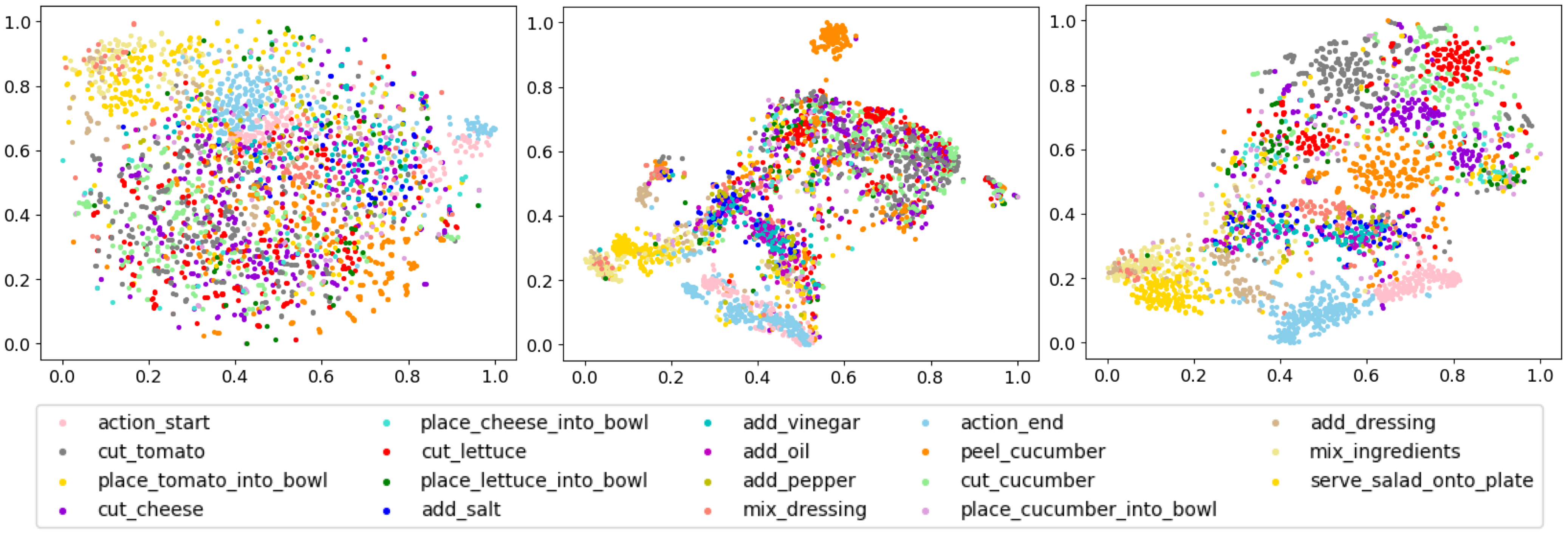
Figure 6: t-SNE visualisation of the I3D feature and other features learned by ICC and our method. Each point represents an image frame. We show all behaviour classes (19) of the 50Salads dataset in different colors.

TABLE VI: Performance of the NCA module on the 50Salads, GTEA and Breakfast datasets (5$\%$).

Dataset	Method	F1@{10, 25, 50}	Edit	Acc
50Salads	w/o $\mathcal{L}_{nca}$	52.1 47.0 35.8	43.9	67.5
	w/ $\mathcal{L}_{nca}$	57.0 53.1 42.1	48.9	68.9
	Gain	4.9  6.1  6.3	5.0	1.4
GTEA	w/o $\mathcal{L}_{nca}$	77.5 74.2 57.7	71.8	71.4
	w/ $\mathcal{L}_{nca}$	81.9 79.3 64.0	77.9	73.9
	Gain	4.4    5.1  6.3	6.1	2.5
Breakfast	w/o $\mathcal{L}_{nca}$	60.8 54.8 39.5	58.1	68.1
	w/ $\mathcal{L}_{nca}$	62.7 57.0 41.6	60.2	68.9
	Gain	1.9   2.2  1.1	2.1	0.8

TABLE VII: Comparing our proposed unsupervised representation learning approach with other existing methods on the 3 benchmarks.

Dataset	Method	F1@{10, 25, 50}	Edit	Acc
50Salads	I3D	12.2   7.9   4.0	8.4	55.0
	ICC[16]	40.8 36.2 28.1	32.4	62.5
	SMC	58.1 54.0 43.5	46.3	75.1
	Gain	17.3 17.8 15.4	13.9	12.6
GTEA	I3D	48.5 42.2 26.4	40.2	61.9
	ICC [16]	70.8 65.0 48.0	65.7	69.1
	SMC	78.9 74.3 59.2	73.0	76.2
	Gain	8.1   9.3 11.2	7.3	7.1
Breakfast	I3D	4.9   2.5   0.9	5.3	30.2
	ICC[16]	57.0 51.7 39.1	51.3	70.5
	SMC	59.7 55.4 42.8	52.7	72.1
	Gain	2.7   3.7   3.7	1.4	1.6

IV-C2 Evaluation of Semi-supervised Learning

Effect of the NCA unit. In Section III-D, we propose the NCA module to alleviate over-segmentation issues when only a fraction of videos are used for semi-supervised learning. Tab. VI shows the results where only 5$\%$ of labelled videos are used for semi-supervised learning on the 50Salads, GTEA and Breakfast datasets. While the baseline without $\mathcal{L}_{nca}$ achieves the expected frame-wise accuracy, it suffers from severe over-segmentation as indicated by the low F1 and Edit scores. By incorporating $\mathcal{L}_{nca}$ within the SMC module, we observe a significant performance boost, up to 6.1$\%$ improvement for the Edit score, and up to 6.3$\%$ improvement for the F1 score on the 50 Salads and GTEA. These results show that our proposed NCA module is capable of reducing over-segmentation errors by identifying the spatial consistency between the action segments. Qualitative results are presented in Fig. 5. Prediction results without the NCA module witness certain over-segmentation errors (numerous small segments), but this issue can be alleviated by our NCA technology that helps identify spatial consistency between neighbourhoods centered at different frames.

Semi-supervised Vs Supervised. We also compare our proposed semi-supervised approach with the supervised counterpart using the same labelled data on the 3 benchmarks, and the results are reported in Tab. V. Performance improvement is noticeable over all the evaluation metrics in both semi-supervised (5$\%$ and 10$\%$) and fully-supervised (100$\%$) setups, confirming the effectiveness of our semi-supervised learning framework.

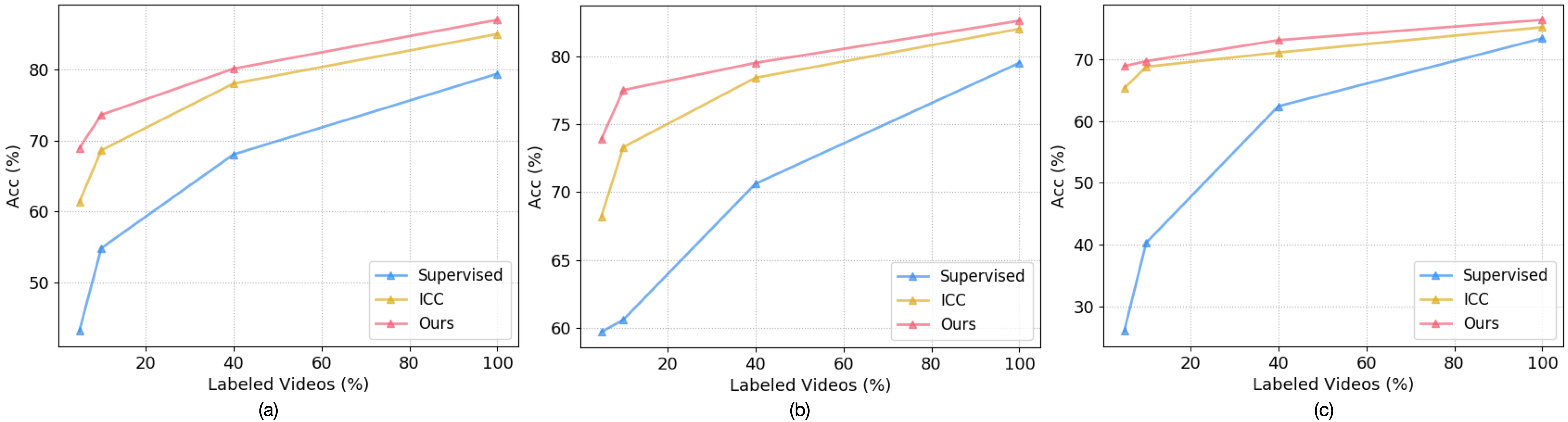
Figure 7: Segmentation accuracy of different methods on (a) 50Salads, (b) GTEA and (c) Breakfast datasets. Our semi-supervised approach continuously achieves satisfactory performance over semi-supervised (5$\%$, 10$\%$ and 40$\%$) and fully-supervised (100$\%$) setups.

TABLE VIII: Comparing our proposed semi-supervised approach with ICC on the 3 benchmarks.

$\%D_{L}$	Method	50salads	GTEA	Breakfast
		F1@{10, 25, 50}  Edit  Acc	F1@{10, 25, 50}  Edit  Acc	F1@{10, 25, 50}  Edit  Acc
5	ICC [16]	52.9 49.0 36.6 45.6 61.3	77.9 71.6 54.6 71.4 68.2	60.2 53.5 35.6 56.6 65.3
	Ours	57.0 53.1 42.1 48.9 68.9	81.9 79.3 64.0 77.9 73.9	62.7 57.0 41.6 60.2 68.9
	Gain	4.1   4.1   5.5   3.3   7.6	4.0   7.7   9.4   6.5   5.7	2.5   3.4   6.0   3.6   3.6
10	ICC [16]	67.3 64.9 49.2 56.9 68.6	83.7 81.9 66.6 76.4 73.3	64.6 59.0 42.2 61.9 68.8
	Ours	70.3 66.3 54.7 61.3 73.6	87.7 84.2 71.7 83.3 77.5	64.8 60.2 45.0 63.4 69.7
	Gain	3.0   1.4   5.5   4.4   5.0	4.0   2.3   5.1   6.9   4.2	0.2   1.2   2.8   1.5   0.9
40	ICC [16]	$\backslash$  $\backslash$  $\backslash$  $\backslash$  78.0	$\backslash$  $\backslash$  $\backslash$  $\backslash$  78.4	$\backslash$  $\backslash$  $\backslash$  $\backslash$  71.1
	Ours	76.5 73.6 65.6 67.9 80.1	85.8 83.6 72.8 80.2 79.5	69.0 64.2 49.5 67.1 73.1
	Gain	$\backslash$  $\backslash$  $\backslash$  $\backslash$    2.1	$\backslash$  $\backslash$  $\backslash$  $\backslash$    1.1	$\backslash$  $\backslash$  $\backslash$  $\backslash$    2.0
100	ICC [16]	83.8 82.0 74.3 76.1 85.0	91.4 89.1 80.5 87.8 82.0	72.4 68.5 55.9 68.6 75.2
	Ours	86.9 84.8 78.9 80.7 87.0	92.7 91.0 81.5 88.3 82.6	73.8 69.7 56.8 70.9 76.4
	Gain	3.1   2.8   4.6   4.6   2.0	1.3   1.9   1.0   0.5   0.6	1.4   1.2   0.9   2.3   1.2

IV-D Comparison against other State-of-the-Art Approaches

In this section, we compare our proposed unsupervised representation learning and semi-supervised learning framework against the other existing methods on three public datasets, i.e., 50 Salads, GTEA and Breakfast datasets and our PDMB dataset. Tabs. VII and IX report the results of the unsupervised representation learning and supervised learning with different levels (i.e., fully-, weakly- and semi-supervised) on the three human action datasets. Tabs. XI and XII show the results on our mouse social behaviour dataset.

As shown in Tab. VII, our SMC is superior to the standard ICC in all the metrics, up to 17.8$\%$ gain for F1 score, 13.9$\%$ gain for Edit score and 12.6$\%$ gain for the frame-wise accuracy on the 50 Salads dataset. We observe a similar tendency on the GTEA dataset, with improvements of 11.2$\%$, 7.3$\%$ and 7.1$\%$ for the F1 score, Edit score and accuracy, respectively. The performance of our SMC mainly attributes to the capture and exploitation of intra- and inter-information variations.

Regarding the Breakfast dataset with complex activities, we keep the video-level contrastive loss in ICC [16] and combine it with our SMC to ensure a fair comparison. The results in Tab. VII show that our approach is marginally better than ICC with respect to all the evaluation metrics. Additionally, as shown in Figs. 6, we visualise the I3D feature and other features learned by ICC and our method using t-Distributed Stochastic Neighbor Embedding (t-SNE) on the 50Salads dataset. Different colors represent different actions in the figures. Our approach leads to better separation of different classes, demonstrating the strong representation learning ability of our Semantic-guided Multi-level Contrast scheme.

TABLE IX: Segmentation accuracy comparison against the state-of-the-art methods under various supervisions on 3 benchmark dataset.

	Method	50Salads	GTEA	Breakfast
Fully	MSTCN[27]	83.7	78.9	67.6
	SSTDA [59]	83.2	79.8	70.2
	C2F-TCN [28]	79.4	79.5	73.4
	ASFormer [31]	85.6	79.7	73.5
	CETNet [60]	86.9	80.3	74.9
	DiffAct [61]	88.9	82.2	76.4
	ICC [16] (100$\%$)	85.0	82.0	75.2
	Ours (100$\%$)	87.0	82.6	76.4
Weakly	SSTDA [59] (65$\%$)	80.7	75.7	65.8
	Timestamp [15]	75.6	66.4	64.1
Semi	ICC [16] (40$\%$)	78.0	78.4	71.1
	Ours (40$\%$)	80.1	79.5	73.1
	ICC [16] (10$\%$)	68.6	73.3	68.8
	Ours (10$\%$)	73.6	77.5	69.7
	ICC [16] (5$\%$)	61.3	68.2	65.3
	Ours (5$\%$)	68.9	73.9	68.9

TABLE X: Comparisons against other semi-supervised learning methods on 5$\%$ labelled data.

Dataset	Method	F1@{10, 25, 50}	Edit	Acc
50Salads	FixMatch [62]	47.0 41.3 28.3	38.3	53.3
	UniMatch [63]	50.3 45.9 30.4	39.7	54.4
	Ours	57.0 53.1 42.1	48.9	68.9
GTEA	FixMatch [62]	69.1 63.9 44.1	59.5	62.0
	UniMatch [63]	65.4 60.0 40.8	57.4	58.7
	Ours	81.9 79.3 64.0	77.9	73.9

In Tab. IX, we show the implementation results of our semi-supervised method using 100$\%$ labelled data, the best frame-wise accuracy among all the fully-supervised approaches. For the semi-supervised setting, we literally perform unsupervised representation learning and semi-supervised classification for 5$\%$, 10$\%$ and 40$\%$ of the training data, and the results show that our framework consistently outperforms ICC by a significant margin. It is noticed that the performance gap (i.e., 7.6$\%$, 5.7$\%$ and 3.6$\%$ improvements in accuracy on the three datasets) between the two methods using only 5$\%$ labelled videos is larger than that using more labelled data. This confirms that our approach is capable of dealing with semi-supervised learning problems in the presence of a small amount of labelled data. As shown in Tab. VIII and Fig. 7, we evaluate our method on three benchmarks and achieve continuously better results for all the performance measures.

We have compared our method with ICC (the most relevant to our work) in Tab. IX. As mentioned in [16], ICC is the first work for semi-supervised action segmentation and is not directly comparable to other works. Most existing image-based semi-supervised learning techniques are not suitable for action segmentation. The reason is that data augmentations (e.g., rotation and transformation) should be applied to input images, but it is non-trivial for action segmentation as the inputs are pre-computed feature vectors [17]. However, we managed to compare our method against two popular semi-supervised learning methods, i.e., FixMatch [62] and UniMatch [63]. In order to reproduce these methods, we designed different data augmentation strategies (e.g., noise) to generate input features with different levels of augmentations. The results reported in Tab. X further verify the superiority of our method.

Temporal dependency modelling is crucial for the detection and segmentation of human actions in long videos [27, 31]. For animal behaviours such as mouse social behaviour recognition in long videos, behavioural correlations are also of importance to infer the social behaviour label of each frame [58]. Therefore, to demonstrate the generalisation and versatility of our proposed framework, we conduct experiments on our Parkinson’s Disease Mouse Behaviour (PDMB) dataset. Tab. XI depicts that our proposed SMC outperforms ICC by a large margin, offering improvement of more than 20$\%$ for all metrics on the PDMB dataset. The reason why ICC has poor performance is that it only exploits temporal information that encodes temporal dependencies of mouse social behaviours to explore the variations of related frames. However, such approach may lead to suboptimal representation learning performance due to complex and diverse behavioural patterns in long videos. In contrast, our proposed SMC integrates both temporal and semantic information, which encodes the behavioural correlations and behaviour-specific characteristics, respectively. By exploiting the intra- and inter-information variations, our framework is able to learn more discriminative frame-wise representations.

We have also compared our entire framework, i.e., SMC-NCA with ICC using different settings of labelled data on our PDMB dataset. As presented in Tab. XII, our approach achieves superior performance over ICC using only 10$\%$, 50$\%$ as well as 100$\%$ labelled data, thus demonstrating the effectiveness of our semi-supervised learning framework in modelling behavioural correlations of mice.

TABLE XI: Comparing our proposed unsupervised representation learning approach with ICC on the PDMB dataset.

Dataset	Method	F1@{10, 25, 50}	Edit	Acc
PDMB	ICC [16]	37.5 32.5 20.6	35.2	40.1
	SMC	61.1 59.6 47.2	55.3	62.5
	Gain	23.6 27.1 26.6	20.3	22.4

TABLE XII: Comparing our proposed framework with ICC on the PDMB dataset.

$\%D_{L}$	Method	PDMB
		F1@{10, 25, 50}  Edit  Acc
10	ICC[16]	50.0 42.5 25.5 49.7 44.5
	Ours	62.0 57.1 40.7 52.7 55.1
	Gain	12.0 14.6 15.2   3.0 10.6
50	ICC[16]	63.5 59.5 40.5 54.4 58.6
	Ours	68.0 63.3 46.6 59.0 66.8
	Gain	4.5   3.8   6.1   4.6   8.2
100	ICC[16]	68.1 63.1 46.1 59.8 69.4
	Ours	71.7 67.5 51.7 63.0 73.6
	Gain	3.6   4.4   5.6   3.2   4.2

Finally, to demonstrate the applicability of the proposed framework to behaviour phenotyping of the mice with Parkinson’s disease, we investigate the behavioural correlations of both MPTP treated mice and their control strains, as shown in Fig. S2. The findings reveal that MPTP treated mice are more likely to perform ’approach’ after ’circle’, ’up’ or ’walk$\_$away’ compared to the control group (’other’ is excluded). Besides, MPTP treated mice tend to exhibit ’sniff’ behaviour while the normal mice show a higher propensity towards ’walk$\_$away’ after ’chase’.

V Conclusions and future work

We have presented SMC-NCA, a novel semantic-guided multi-level contrast framework that aims to yield more discriminative frame-wise representations by fully exploiting complementary information from semantic and temporal entities. The proposed SMC aims to explore intra- and inter-information variations for unsupervised representation learning by integrating both semantic and temporal information. To achieve this goal, three types of dense negative pairs are explicitly constructed to facilitate contrastive learning. Our SMC provides a comprehensive solution that leverages both semantic and temporal features to enable effective unsupervised representation learning for action segmentation. To alleviate the over-segmentation problems in the semi-supervised setting with only a small amount of labelled data, the NCA module fully utilises spatial consistency between the neighbourhoods centered at different frames. Our framework outperforms the other state-of-the-art approaches on the three public datasets and our PDMB dataset, which demonstrates the generalisation and versatility of our proposed framework for the datasets of different domains. However, for the dataset with video-level activity labels such as Breakfast, our multi-level contrast framework needs to be further developed in order to handle the similarity of activities over the image frames. We will leave this exploration as future work.

Supplementary A

Additional Visualization. As shown in Fig. S1, we visualise the I3D feature and other features learned by ICC and our method using t-Distributed Stochastic Neighbor Embedding (t-SNE) on GTEA datasets. Different colours represent different actions. Our approach leads to better separation of different classes, demonstrating the strong representation learning ability of our Semantic-guided Multi-level Contrast scheme.

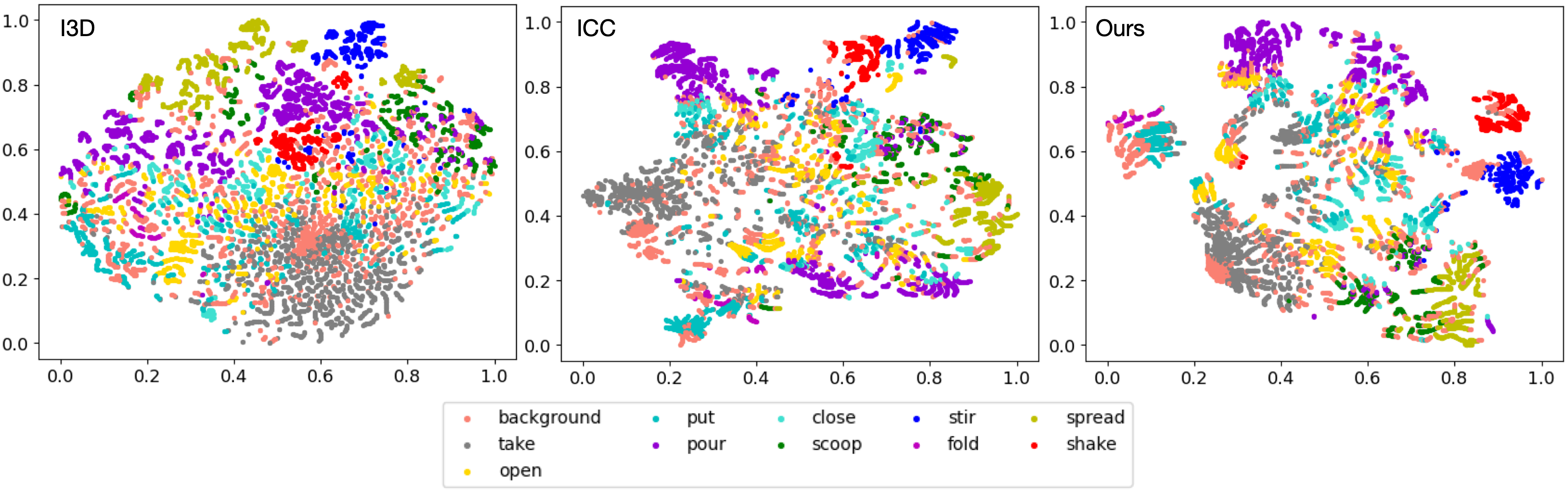
Figure S1: t-SNE visualisation of the I3D feature and other features learned by ICC and our method. Each point represents an image frame. We show all behaviour classes (11) of the GTEA dataset in different colours.

Compare SMC with other unsupervised representation learning methods. In Tab. 3 (main paper) of the paper, we have compared our unsupervised method with that of ICC. Since ICC is the first work based on unsupervised representation learning for semi-supervised action segmentation, so far we could not find any other publications exploring unsupervised representation learning for this task. Thus, we attempt to compare our unsupervised method against a SOTA method [39] of unsupervised video representation learning, but it is not quite related to this task. We use the same positive and anchor representations as those of our work but the negative representation is obtained by temporal shuffling [39] of anchor representation. From Tab. S1, our method shows better performance.

TABLE S1: Comparing Our SMC with SCVRL [39].

Dataset	Method	F1@{10, 25, 50}	Edit	Acc
50Salads	SCVRL [39]	48.0 43.5 34.4	37.8	69.2
	SMC	58.1 54.0 43.5	46.3	75.1
GTEA	SCVRL [39]	72.5 66.0 48.6	64.9	71.2
	SMC	78.9 74.3 59.2	73.0	76.2
Breakfast	SCVRL[39]	46.8 41.9 31.8	38.6	71.1
	SMC	59.7 55.4 42.8	52.7	72.1

Supplementary B

TABLE S2: Ethogram of the observed behaviours [58].

Behaviour	Description
approach	Moving toward another mouse in a straight line without obvious exploration.
chase	A following mouse attempts to maintain a close distance to another mouse while the latter is moving.
circle	Circling around own axis or chasing tail.
eat	Gnawing/eating food pellets held by the fore-paws.
clean	Washing the muzzle with fore-paws (including licking fore-paws) or grooming the fur or hind-paws by means of licking or chewing.
sniff	Sniff any body part of another mouse.
up	Exploring while standing in an upright posture.
walk away	Moving away from another mouse in a straight line without obvious exploration.
other	ehaviour other than defined in this ethogram, or when it is not visible what behaviour the mouse displays.

Additional related works about temporal modelling of mouse behaviour. In recent years, temporal dependencies among actions have also been investigated to facilitate mouse behaviour modelling. Jiang et al. [64] employed a Hidden Markov Model (HMM) to model the contextual relationship among adjacent mouse behaviours over time. Specifically, they represented each action clip as a set of feature vectors using spatial-temporal Segment Fisher Vectors (SFV), which were then treated as observed variables in the HMM. In addition, Jiang et al. [58] proposed a deep graphic model to explore the temporal correlations of mouse social behaviours, which demonstrated the advantage of modelling behavioural correlations. However, these methods mainly focus on the correlations between the neighbouring behaviours, which is difficult to capture multi-scale temporal dependencies of mouse behaviours in long videos. Also, these methods usually require fully supervised data, which is obtained by manually annotating the exact temporal location of each behaviour occurring in all training videos. Such data collection is expensive, particularly in behavioural neuroscience [65], where datasets are usually complex and lab-specific.

TABLE S3: Component-wise analysis of the unsupervised representation learning framework with a linear classifier on the PDMB dataset.

Method	PDMB
	F1@{10, 25, 50}   Edit   Acc
$\mathcal{L}_{ap}^{P}$($\textbf{M}_{in}$)+$\mathcal{L}_{aa}^{N}$	39.0  33.9 21.6  36.5  37.7
$\mathcal{L}_{ap}^{P}$(I)+$\mathcal{L}_{aa}^{N}$	56.3  53.6 40.8  51.8  53.4
$\mathcal{L}_{ap}^{P}$($\textbf{M}_{in}$)+$\mathcal{L}_{ap}^{N}$	38.0  34.2 24.3  35.3  42.2
$\mathcal{L}_{ap}^{P}$(I)+$\mathcal{L}_{ap}^{N}$	55.9  53.5 41.0  40.1  54.3
Constructing positive pairs by $\textbf{M}_{in}$ or $I$
$\mathcal{L}_{ap}^{P}$ + $\mathcal{L}_{aa}^{N}$	56.3  53.6 40.8  51.8  53.4
$\mathcal{L}_{ap}^{P}$ + $\mathcal{L}_{ap}^{N}$	55.9  53.5 41.0  40.1  54.3
$\mathcal{L}_{ap}^{P}$ + $\mathcal{L}_{aa}^{N}$ + $\mathcal{L}_{ap}^{N}$	58.5  56.6 43.6  53.4  58.5
$\mathcal{L}_{ap}^{P}$ + $\mathcal{L}_{aa}^{N}$ + $\mathcal{L}_{ap}^{N}$ + $\mathcal{L}_{pp}^{N}$	59.6  58.0 45.9  53.8  61.3
Comparing different negative pairs
w/o dynamic clustering	59.6  58.0 45.9  53.8  61.3
w/ dynamic clustering	61.1  59.6 47.2  55.5  62.5
Dynamic clustering facilitates contrastive learning

TABLE S4: Performance of the NCA module on our PDMB dataset (10$\%$).

Dataset	Method	F1@{10, 25, 50}	Edit	Acc
PDMB	w/o $\mathcal{L}_{nca}$	54.7 48.7 31.9	45.0	52.7
	w/ $\mathcal{L}_{nca}$	62.0 57.1 40.7	52.7	55.1
	Gain	7.3   8.4  8.8	7.7	2.4

Mouse Social Behaviour Dataset. Our Parkinson’s Disease Mouse Behaviour (PDMB) dataset was collected in collaboration with the biologists of Queen’s University Belfast of United Kingdom, for a study on motion recordings of mice with Parkinson’s disease (PD) [58]. The neurotoxin 1-methyl-4-phenyl-1,2,3,6-tetrahydropyridine (MPTP) is used as a model of PD, which has become an invaluable aid to produce experimental parkinsonism since its discovery in 1983 [66]. All experimental procedures were performed in accordance with the Guidance on the Operation of the Animals (Scientific Procedures) Act, 1986 (UK) and approved by the Queen’s University Belfast Animal Welfare and Ethical Review Body. We recorded videos for 3 groups of MPTP treated mice and 3 groups of control mice by using three synchronised Sony Action cameras (HDR-AS15) (one top-view and two side-view) with frame rate of 30 fps and 640*480 resolution. Each group consists of 6 annotated videos and all videos contain 9 behaviours (defined in Tab. S2) of two freely behaving mice. Different from the experiments of human action segmentation, the input features we use in experiments on this dataset are extracted from the pre-trained model from [67], which encodes the social interactions of mice based on the pose information [57]. The whole dataset is evenly divided into training and testing datasets, and we select 10$\%$ or 50$\%$ of the videos from the training split for the labelled dataset $\mathcal{D}_{L}$.

Evaluation of Representation Learning on the PDMB Dataset. As shown in Tab. S3, on the PDMB dataset, utilising $\textbf{M}_{in}$ would also lead to the generation of pseudo positive pairs, which would impede the efficacy of contrastive learning and consequently result in a significant performance drop. Besides, we achieve the best performance for all metrics when combining three types of negative pairs at the same time, where such combination brings gains of 7.9$\%$ and 7$\%$ in accuracy for the settings with only $\mathcal{L}_{aa}^{N}$ and $\mathcal{L}_{ap}^{N}$, respectively.

Effect of the NCA Unit on the PDMB Dataset. As shown in Tab. S4, with respect to behavioural correlation modelling of mice, we achieve a significant improvement of more than 7$\%$ in F1 and Edit scores on the PDMB dataset.

Finally, to demonstrate the applicability of the proposed framework to behaviour phenotyping of the mice with Parkinson’s disease, we investigate the behavioural correlations of both MPTP treated mice and their control strains, as shown in Fig. S2. The findings reveal that MPTP treated mice are more likely to perform ’approach’ after ’circle’, ’up’ or ’walk$\_$away’ compared to the control group (’other’ is excluded). Besides, MPTP treated mice tend to exhibit ’sniff’ behaviour while the normal mice show a higher propensity towards ’walk$\_$away’ after ’chase’.

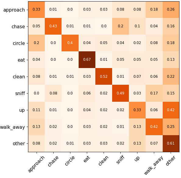
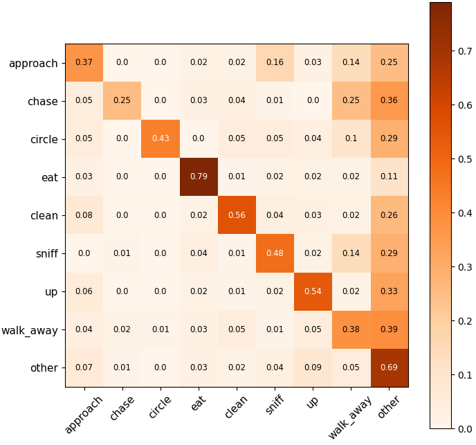
(a) Parkinson’s Disease mice	(b) Normal mice

Figure S2: Occurrence frequency of neighbouring behaviours (20-frame interval) for Parkinson’s Disease and normal mice. Each cell contains the percentage of the occurrence of behaviour x (along rows) after behaviour y (along column) appears.

References

- [1] Z. Li, J. Li, Y. Ma, R. Wang, Z. Shi, Y. Ding, and X. Liu, “Spatio-temporal adaptive network with bidirectional temporal difference for action recognition,” IEEE Transactions on Circuits and Systems for Video Technology, 2023.
- [2] Y. Chen, H. Ge, Y. Liu, X. Cai, and L. Sun, “Agpn: Action granularity pyramid network for video action recognition,” IEEE Transactions on Circuits and Systems for Video Technology, 2023.
- [3] H. Wu, X. Ma, and Y. Li, “Spatiotemporal multimodal learning with 3d cnns for video action recognition,” IEEE Transactions on Circuits and Systems for Video Technology, vol. 32, no. 3, pp. 1250–1261, 2021.
- [4] H. Wang, B. Yu, J. Li, L. Zhang, and D. Chen, “Multi-stream interaction networks for human action recognition,” IEEE Transactions on Circuits and Systems for Video Technology, vol. 32, no. 5, pp. 3050–3060, 2021.
- [5] H. Luo, G. Lin, Y. Yao, Z. Tang, Q. Wu, and X. Hua, “Dense semantics-assisted networks for video action recognition,” IEEE Transactions on Circuits and Systems for Video Technology, vol. 32, no. 5, pp. 3073–3084, 2021.
- [6] C. Lea, M. D. Flynn, R. Vidal, A. Reiter, and G. D. Hager, “Temporal convolutional networks for action segmentation and detection,” in proceedings of the IEEE Conference on Computer Vision and Pattern Recognition, 2017, pp. 156–165.
- [7] Q. Shi, L. Cheng, L. Wang, and A. Smola, “Human action segmentation and recognition using discriminative semi-markov models,” International journal of computer vision, vol. 93, pp. 22–32, 2011.
- [8] S.-J. Li, Y. AbuFarha, Y. Liu, M.-M. Cheng, and J. Gall, “Ms-tcn++: Multi-stage temporal convolutional network for action segmentation,” IEEE transactions on pattern analysis and machine intelligence, 2020.
- [9] J. Li, P. Lei, and S. Todorovic, “Weakly supervised energy-based learning for action segmentation,” in Proceedings of the IEEE/CVF International Conference on Computer Vision, 2019, pp. 6243–6251.
- [10] Z. Lu and E. Elhamifar, “Weakly-supervised action segmentation and alignment via transcript-aware union-of-subspaces learning,” in Proceedings of the IEEE/CVF International Conference on Computer Vision, 2021, pp. 8085–8095.
- [11] Y. Souri, M. Fayyaz, L. Minciullo, G. Francesca, and J. Gall, “Fast weakly supervised action segmentation using mutual consistency,” IEEE Transactions on Pattern Analysis and Machine Intelligence, 2021.
- [12] A. Richard, H. Kuehne, and J. Gall, “Action sets: Weakly supervised action segmentation without ordering constraints,” in Proceedings of the IEEE conference on Computer Vision and Pattern Recognition, 2018, pp. 5987–5996.
- [13] J. Li and S. Todorovic, “Set-constrained viterbi for set-supervised action segmentation,” in Proceedings of the IEEE/CVF Conference on Computer Vision and Pattern Recognition, 2020, pp. 10 820–10 829.
- [14] M. Fayyaz and J. Gall, “Sct: Set constrained temporal transformer for set supervised action segmentation,” in Proceedings of the IEEE/CVF Conference on Computer Vision and Pattern Recognition, 2020, pp. 501–510.
- [15] Z. Li, Y. Abu Farha, and J. Gall, “Temporal action segmentation from timestamp supervision,” in Proceedings of the IEEE/CVF Conference on Computer Vision and Pattern Recognition, 2021, pp. 8365–8374.
- [16] D. Singhania, R. Rahaman, and A. Yao, “Iterative contrast-classify for semi-supervised temporal action segmentation,” in Proceedings of the AAAI Conference on Artificial Intelligence, vol. 36, 2022, pp. 2262–2270.
- [17] G. Ding and A. Yao, “Leveraging action affinity and continuity for semi-supervised temporal action segmentation,” arXiv preprint arXiv:2207.08653, 2022.
- [18] D. Singhania, R. Rahaman, and A. Yao, “C2f-tcn: A framework for semi-and fully-supervised temporal action segmentation,” IEEE Transactions on Pattern Analysis and Machine Intelligence, 2023.
- [19] T. Chen, S. Kornblith, M. Norouzi, and G. Hinton, “A simple framework for contrastive learning of visual representations,” in International conference on machine learning. PMLR, 2020, pp. 1597–1607.
- [20] L. Tao, X. Wang, and T. Yamasaki, “An improved inter-intra contrastive learning framework on self-supervised video representation,” IEEE Transactions on Circuits and Systems for Video Technology, vol. 32, no. 8, pp. 5266–5280, 2022.
- [21] F. Schroff, D. Kalenichenko, and J. Philbin, “Facenet: A unified embedding for face recognition and clustering,” in Proceedings of the IEEE conference on computer vision and pattern recognition, 2015, pp. 815–823.
- [22] W. Xie, H. Wu, Y. Tian, M. Bai, and L. Shen, “Triplet loss with multistage outlier suppression and class-pair margins for facial expression recognition,” IEEE Transactions on Circuits and Systems for Video Technology, vol. 32, no. 2, pp. 690–703, 2021.
- [23] J.-Y. Franceschi, A. Dieuleveut, and M. Jaggi, “Unsupervised scalable representation learning for multivariate time series,” Advances in neural information processing systems, vol. 32, 2019.
- [24] Y. Ishikawa, S. Kasai, Y. Aoki, and H. Kataoka, “Alleviating over-segmentation errors by detecting action boundaries,” in Proceedings of the IEEE/CVF winter conference on applications of computer vision, 2021, pp. 2322–2331.
- [25] H. Kuehne, J. Gall, and T. Serre, “An end-to-end generative framework for video segmentation and recognition,” in 2016 IEEE Winter Conference on Applications of Computer Vision (WACV). IEEE, 2016, pp. 1–8.
- [26] B. Singh, T. K. Marks, M. Jones, O. Tuzel, and M. Shao, “A multi-stream bi-directional recurrent neural network for fine-grained action detection,” in Proceedings of the IEEE conference on computer vision and pattern recognition, 2016, pp. 1961–1970.
- [27] Y. A. Farha and J. Gall, “Ms-tcn: Multi-stage temporal convolutional network for action segmentation,” in Proceedings of the IEEE/CVF Conference on Computer Vision and Pattern Recognition, 2019, pp. 3575–3584.
- [28] D. Singhania, R. Rahaman, and A. Yao, “Coarse to fine multi-resolution temporal convolutional network,” arXiv preprint arXiv:2105.10859, 2021.
- [29] Y. Huang, Y. Sugano, and Y. Sato, “Improving action segmentation via graph-based temporal reasoning,” in Proceedings of the IEEE/CVF conference on computer vision and pattern recognition, 2020, pp. 14 024–14 034.
- [30] D. Wang, D. Hu, X. Li, and D. Dou, “Temporal relational modeling with self-supervision for action segmentation,” in Proceedings of the AAAI Conference on Artificial Intelligence, vol. 35, 2021, pp. 2729–2737.
- [31] F. Yi, H. Wen, and T. Jiang, “Asformer: Transformer for action segmentation,” arXiv preprint arXiv:2110.08568, 2021.
- [32] A. Kukleva, H. Kuehne, F. Sener, and J. Gall, “Unsupervised learning of action classes with continuous temporal embedding,” in Proceedings of the IEEE/CVF Conference on Computer Vision and Pattern Recognition, 2019, pp. 12 066–12 074.
- [33] S. Sarfraz, N. Murray, V. Sharma, A. Diba, L. Van Gool, and R. Stiefelhagen, “Temporally-weighted hierarchical clustering for unsupervised action segmentation,” in Proceedings of the IEEE/CVF Conference on Computer Vision and Pattern Recognition, 2021, pp. 11 225–11 234.
- [34] S. Kumar, S. Haresh, A. Ahmed, A. Konin, M. Z. Zia, and Q.-H. Tran, “Unsupervised action segmentation by joint representation learning and online clustering,” in Proceedings of the IEEE/CVF Conference on Computer Vision and Pattern Recognition, 2022, pp. 20 174–20 185.
- [35] G. Ding and A. Yao, “Temporal action segmentation with high-level complex activity labels,” IEEE Transactions on Multimedia, 2022.
- [36] K. He, H. Fan, Y. Wu, S. Xie, and R. Girshick, “Momentum contrast for unsupervised visual representation learning,” in Proceedings of the IEEE/CVF conference on computer vision and pattern recognition, 2020, pp. 9729–9738.
- [37] A. v. d. Oord, Y. Li, and O. Vinyals, “Representation learning with contrastive predictive coding,” arXiv preprint arXiv:1807.03748, 2018.
- [38] Y. Tian, D. Krishnan, and P. Isola, “Contrastive multiview coding,” in European conference on computer vision. Springer, 2020, pp. 776–794.
- [39] M. Dorkenwald, F. Xiao, B. Brattoli, J. Tighe, and D. Modolo, “Scvrl: Shuffled contrastive video representation learning,” in Proceedings of the IEEE/CVF Conference on Computer Vision and Pattern Recognition, 2022, pp. 4132–4141.
- [40] K. Hu, J. Shao, Y. Liu, B. Raj, M. Savvides, and Z. Shen, “Contrast and order representations for video self-supervised learning,” in Proceedings of the IEEE/CVF International Conference on Computer Vision, 2021, pp. 7939–7949.
- [41] R. Qian, T. Meng, B. Gong, M.-H. Yang, H. Wang, S. Belongie, and Y. Cui, “Spatiotemporal contrastive video representation learning,” in Proceedings of the IEEE/CVF Conference on Computer Vision and Pattern Recognition, 2021, pp. 6964–6974.
- [42] A. Recasens, P. Luc, J.-B. Alayrac, L. Wang, F. Strub, C. Tallec, M. Malinowski, V. Pătrăucean, F. Altché, M. Valko et al., “Broaden your views for self-supervised video learning,” in Proceedings of the IEEE/CVF International Conference on Computer Vision, 2021, pp. 1255–1265.
- [43] S. Biswas and J. Gall, “Multiple instance triplet loss for weakly supervised multi-label action localisation of interacting persons,” in Proceedings of the IEEE/CVF International Conference on Computer Vision, 2021, pp. 2159–2167.
- [44] Y. Zhu, H. Shuai, G. Liu, and Q. Liu, “Self-supervised video representation learning using improved instance-wise contrastive learning and deep clustering,” IEEE Transactions on Circuits and Systems for Video Technology, vol. 32, no. 10, pp. 6741–6752, 2022.
- [45] E. Eldele, M. Ragab, Z. Chen, M. Wu, C. K. Kwoh, X. Li, and C. Guan, “Time-series representation learning via temporal and contextual contrasting,” arXiv preprint arXiv:2106.14112, 2021.
- [46] Z. Yue, Y. Wang, J. Duan, T. Yang, C. Huang, Y. Tong, and B. Xu, “Ts2vec: Towards universal representation of time series,” in Proceedings of the AAAI Conference on Artificial Intelligence, vol. 36, 2022, pp. 8980–8987.
- [47] W. Ge, “Deep metric learning with hierarchical triplet loss,” in Proceedings of the European Conference on Computer Vision (ECCV), 2018, pp. 269–285.
- [48] F. Boutros, N. Damer, F. Kirchbuchner, and A. Kuijper, “Self-restrained triplet loss for accurate masked face recognition,” Pattern Recognition, vol. 124, p. 108473, 2022.
- [49] S. Chen, X. Zhu, Y. Yan, S. Zhu, S.-Z. Li, and D.-H. Wang, “Identity-aware contrastive knowledge distillation for facial attribute recognition,” IEEE Transactions on Circuits and Systems for Video Technology, 2023.
- [50] J. Carreira and A. Zisserman, “Quo vadis, action recognition? a new model and the kinetics dataset,” in proceedings of the IEEE Conference on Computer Vision and Pattern Recognition, 2017, pp. 6299–6308.
- [51] Z. Ming, J. Chazalon, M. M. Luqman, M. Visani, and J.-C. Burie, “Simple triplet loss based on intra/inter-class metric learning for face verification,” in 2017 IEEE International Conference on Computer Vision Workshops (ICCVW). IEEE, 2017, pp. 1656–1664.
- [52] P. Zhang, C. Lan, W. Zeng, J. Xing, J. Xue, and N. Zheng, “Semantics-guided neural networks for efficient skeleton-based human action recognition,” in proceedings of the IEEE/CVF conference on computer vision and pattern recognition, 2020, pp. 1112–1121.
- [53] F. Sener, D. Singhania, and A. Yao, “Temporal aggregate representations for long-range video understanding,” in European Conference on Computer Vision. Springer, 2020, pp. 154–171.
- [54] S. Stein and S. J. McKenna, “Combining embedded accelerometers with computer vision for recognizing food preparation activities,” in Proceedings of the 2013 ACM international joint conference on Pervasive and ubiquitous computing, 2013, pp. 729–738.
- [55] A. Fathi, X. Ren, and J. M. Rehg, “Learning to recognize objects in egocentric activities,” in CVPR 2011. IEEE, 2011, pp. 3281–3288.
- [56] H. Kuehne, A. Arslan, and T. Serre, “The language of actions: Recovering the syntax and semantics of goal-directed human activities,” in Proceedings of the IEEE conference on computer vision and pattern recognition, 2014, pp. 780–787.
- [57] F. Zhou, Z. Jiang, Z. Liu, F. Chen, L. Chen, L. Tong, Z. Yang, H. Wang, M. Fei, L. Li et al., “Structured context enhancement network for mouse pose estimation,” IEEE Transactions on Circuits and Systems for Video Technology, vol. 32, no. 5, pp. 2787–2801, 2021.
- [58] Z. Jiang, F. Zhou, A. Zhao, X. Li, L. Li, D. Tao, X. Li, and H. Zhou, “Multi-view mouse social behaviour recognition with deep graphic model,” IEEE Transactions on Image Processing, vol. 30, pp. 5490–5504, 2021.
- [59] M.-H. Chen, B. Li, Y. Bao, G. AlRegib, and Z. Kira, “Action segmentation with joint self-supervised temporal domain adaptation,” in Proceedings of the IEEE/CVF Conference on Computer Vision and Pattern Recognition, 2020, pp. 9454–9463.
- [60] J. Wang, Z. Wang, S. Zhuang, and H. Wang, “Cross-enhancement transformer for action segmentation,” arXiv preprint arXiv:2205.09445, 2022.
- [61] D. Liu, Q. Li, A. Dinh, T. Jiang, M. Shah, and C. Xu, “Diffusion action segmentation,” in Proceedings of the IEEE/CVF International Conference on Computer Vision, 2023.
- [62] K. Sohn, D. Berthelot, N. Carlini, Z. Zhang, H. Zhang, C. A. Raffel, E. D. Cubuk, A. Kurakin, and C.-L. Li, “Fixmatch: Simplifying semi-supervised learning with consistency and confidence,” Advances in neural information processing systems, vol. 33, pp. 596–608, 2020.
- [63] L. Yang, L. Qi, L. Feng, W. Zhang, and Y. Shi, “Revisiting weak-to-strong consistency in semi-supervised semantic segmentation,” in Proceedings of the IEEE/CVF Conference on Computer Vision and Pattern Recognition, 2023, pp. 7236–7246.
- [64] Z. Jiang, D. Crookes, B. D. Green, Y. Zhao, H. Ma, L. Li, S. Zhang, D. Tao, and H. Zhou, “Context-aware mouse behavior recognition using hidden markov models,” IEEE Transactions on Image Processing, vol. 28, no. 3, pp. 1133–1148, 2018.
- [65] T. D. Pereira, J. W. Shaevitz, and M. Murthy, “Quantifying behavior to understand the brain,” Nature neuroscience, vol. 23, no. 12, pp. 1537–1549, 2020.
- [66] V. Jackson-Lewis and S. Przedborski, “Protocol for the mptp mouse model of parkinson’s disease,” Nature protocols, vol. 2, no. 1, p. 141, 2007.
- [67] F. Zhou, X. Yang, F. Chen, L. Chen, Z. Jiang, H. Zhu, R. Heckel, H. Wang, M. Fei, and H. Zhou, “Cross-skeleton interaction graph aggregation network for representation learning of mouse social behaviour,” arXiv preprint arXiv:2208.03819, 2022.