Scalable Near-Field Localization Based on Array Partitioning and Angle-of-Arrival Fusion

Abstract

Existing near-field localization algorithms generally face a scalability issue when the number of antennas at the sensor array goes large. To address this issue, this paper studies a passive localization system, where an extremely large-scale antenna array (ELAA) is deployed at the base station (BS) to locate a user that transmits signals. The user is considered to be in the near-field (Fresnel) region of the BS array. We propose a novel algorithm, named array partitioning based location estimation (APLE), for scalable near-field localization. The APLE algorithm is developed based on the basic assumption that, by partitioning the ELAA into multiple subarrays, the user can be approximated as in the far-field region of each subarray. The APLE algorithm determines the user’s location by exploiting the differences in the angles of arrival (AoAs) of the subarrays. Specifically, we establish a probability model of the received signal based on the geometric constraints of the user’s location and the observed AoAs. Then, a message-passing algorithm, i.e., the proposed APLE algorithm, is designed for user localization. APLE exhibits linear computational complexity with the number of BS antennas, leading to a significant reduction in complexity compared to the existing methods. Besides, numerical results demonstrate that the proposed APLE algorithm outperforms the existing baselines in terms of localization accuracy.

I Introduction

The fusion of sensing and communication systems, known as integrated sensing and communication (ISAC), has emerged as a promising research direction for sixth-generation (6G) mobile communications. This fusion is driven by the growing demand for high-quality communication and sensing services in various emerging 6G application scenarios, such as augmented reality (AR), internet of vehicles (IoV), and unmanned aerial vehicle (UAV) communications. In these applications, efficient and precise acquisition of user location information is of critical importance, with centimeter-level localization accuracy expected for ensuring required service quality[1, 2]. Much research effort has been devoted to leveraging emerging 6G technologies, such as Terahertz communication, intelligent reflecting surface (IRS), and extremely large-scale multi-input-multi-output (XL-MIMO) to provide enhanced localization services in 6G[3, 4].

Among these new technologies, XL-MIMO is considered to have the potential to greatly improve the localization capabilities of wireless networks. To meet the demands for higher spectral efficiency and larger system capacity in 6G networks, the utilization of a larger antenna array than what is currently used in fifth-generation (5G) mobile communications has become a realistic trend[5]. Compared with massive MIMO which involves up to hundreds of antennas deployed at base station (BS), 6G XL-MIMO is expected to employ extremely large-scale antenna arrays (ELAAs) comprising thousands or even tens of thousands of antennas[6]. The deployment of ELAA enables the anchors to collect enough measurements even in one snapshot, thereby enhancing the preciseness and robustness of wireless localization[7].

There are, however, many challenging issues to be addressed before wireless localization can reap the full benefits of XL-MIMO. First of all, in traditional localization problems, sources are typically located in the far-field region of an antenna array, such that the array can only discriminate the angles of arrival (AoAs) of impinging electromagnetic waves, but can not locate the exact positions of the sources. However, in XL-MIMO, due to the expanded aperture of the BS ELAA, sources are more likely to be located in the near-field region (also known as the Fresnel region) of the BS ELAA. Consequently, the localization task now requires the BS to simultaneously estimate both the target’s direction and its distance from the BS.

Near-field localization has been intensively studied in the past few years [8, 9, 10, 11, 12]. Yet, these existing near-field localization algorithms generally suffer from scalability issues when applied to XL-MIMO scenarios. The vast number of antennas in ELAA significantly increases the dimensionality of the received signal, resulting in extremely high computational complexities for the existing localization algorithms. Take the well-known multiple signal classification (MUSIC) algorithm[10] as an example. The complexity of the MUSIC algorithm primarily arises from the eigen decomposition of the received signal correlation matrix, where the complexity increases cubically with the number of antennas. In the case of ELAA, where the number of antennas can reach thousands or even tens of thousands, this cubic complexity leads to a prohibitively high computational burden for the receiver. Other high-precision near-field localization algorithms, such as those based on estimation of signal parameters via rotational invariance technique (ESPRIT) and compressed sensing[11, 12], also exhibit cubic or even higher complexities with the number of antennas. As such, it is of crucial importance to develop accurate yet scalable near-field localization algorithms for XL-MIMO systems.

To tackle this issue, we propose a novel algorithm for scalable near-field localization, named array partitioning based location estimation (APLE) algorithm. Specifically, we consider a passive localization system, where an ELAA is deployed at the BS to locate a user in the near-field region using the received signal. The proposed APLE algorithm is designed based on the basic assumption that, by partitioning the ELAA into multiple subarrays, the user can be approximated as in the far-field region of each subarray. Owing to a distinct relative position between each subarray and the user, the signal transmitted by the user exhibits varying AoAs as they arrive at different subarrays, known as AoA drifting. The APLE algorithm leverages the AoA drifting effect for user localization. Specifically, a probability model of the received signal is established based on the geometric constraints of the user’s location and the observed AoAs. Based on a factor graph representation of this probability model, a message-passing algorithm, namely the proposed APLE algorithm, is designed to estimate the user’s location. Approximations are introduced to simplify message calculations in APLE. The APLE algorithm exhibits nearly linear complexity with the number of BS antennas and achieves a complexity reduction in orders of magnitude as compared to the existing near-field localization algorithms. Besides, numerical results demonstrate that the APLE algorithm outperforms many baselines in terms of localization accuracy. In the high signal-to-noise ratio (SNR) regime, its performance closely approaches the lower bound (LB) provided by the misspecified Cramér-Rao bound (MCRB) analysis[13] of the considered localization problem.

II System Model

Consider an uplink communication system as illustrated in Fig. 1. The BS is equipped with an $N_{\mathrm{B}}$-antenna ELAA arranged as a uniform planar array (UPA) and the user is equipped with a single antenna. A 3D Cartesian coordinate system is established with the center of the BS array as the origin $O$. The $x$-axis and the $y$-axis are parallel to the two sides of the BS array, and the $z$-axis is perpendicular to the BS array. We assume $N_{\mathrm{B}}=N_{\mathrm{x}}\times N_{\mathrm{y}}$, where $N_{\mathrm{x}}$ and $N_{\mathrm{y}}$ are the number of antennas along the $x$-axis and $y$-axis, respectively. For ease of notation, $N_{\mathrm{x}}$ and $N_{\mathrm{y}}$ are assumed to be odd numbers. The uniform antenna spacings of the BS array along the $x$-axis and $y$-axis are denoted by $d_{\mathrm{x}}$ and $d_{\mathrm{y}}$, respectively. The size of the BS array is given by $L_{\mathrm{x}}\times L_{\mathrm{y}}$, where $L_{\mathrm{x}}=N_{\mathrm{x}}d_{\mathrm{x}}$ and $L_{\mathrm{y}}=N_{\mathrm{y}}d_{\mathrm{y}}$. Denote by $\mathcal{I}_{N}=\{-\frac{N-1}{2},\ldots,\frac{N-1}{2}\}$ the index set, where $N$ is a odd number. Denote by $\mathbf{p}_{\mathrm{BS},(i,j)}=[id_{\mathrm{x}},jd_{\mathrm{y}},0]^{\mathrm{T}}$ the location of the $(i,j)$-th antenna at the BS array, $i\in\mathcal{I}_{N_{\mathrm{x}}}$, $j\in\mathcal{I}_{N_{\mathrm{y}}}$, where $\mathbf{p}_{\mathrm{BS}}=\boldsymbol{0}$ corresponds to the center of the BS array. Deonte by $\mathbf{p}_{\mathrm{U}}=[x,y,z]^{\mathrm{T}}$ the location of the user, and by $r=\left\|\mathbf{p}_{\mathrm{U}}-\mathbf{p}_{\mathrm{BS}}\right\|$ the link distance between the user and the center of the BS array.

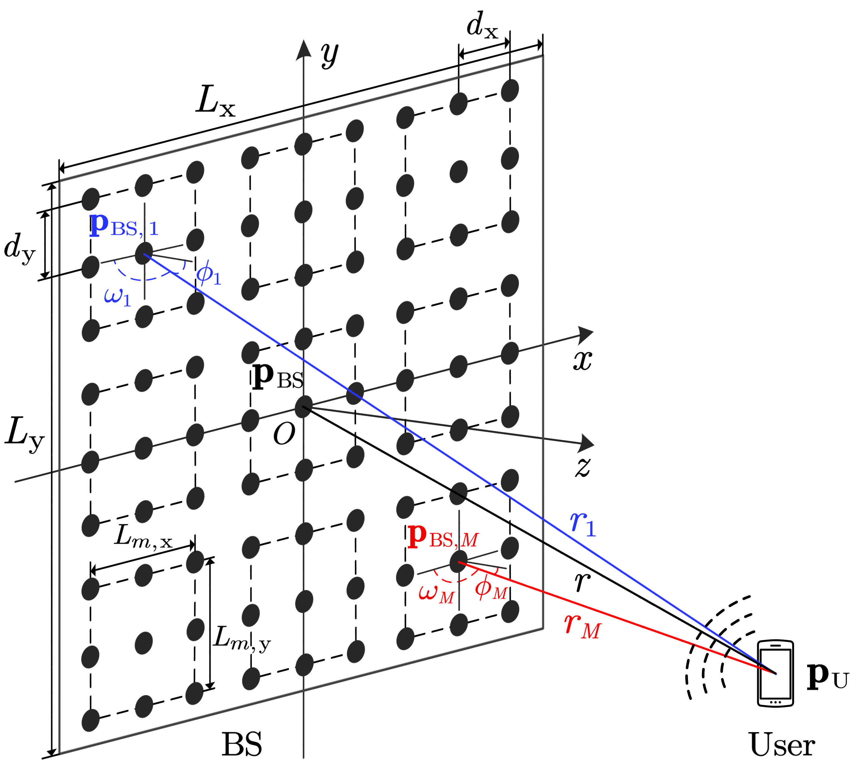
Figure 1: The uplink communication system with the user located in the near-field region of the BS array.

We assume that the user is located in the near-field region of the BS array, i.e., $R_{\mathrm{N}}<r<R_{\mathrm{F}}$, where $R_{\mathrm{N}}\triangleq 0.62\sqrt{{D^{3}}/{\lambda}}$ and $R_{\mathrm{F}}\triangleq{2D^{2}}/{\lambda}$ are the Fresnel distance and the Fraunhofer distance[14], respectively, and $D\triangleq\left(L_{\mathrm{x}}^{2}+L_{\mathrm{y}}^{2}\right)^{\frac{1}{2}}$ represents the largest dimension of the BS array. Furthermore, we assume that the considered near-field channel only consists of line-of-sight (LoS) components. As shown in Fig. 1, the LoS paths from the user to the BS antennas have different propagation distances. In this case, we model the near-field LoS channel with the exact propagation distances by considering the free-space transmission. Denote by $r_{(i,j)}=\left\|\mathbf{p}_{\mathrm{BS},(i,j)}-\mathbf{p}_{\mathrm{U}}\right\|$ the propagation distance between the user and the $(i,j)$-th antenna of the BS array, $i\in\mathcal{I}_{N_{\mathrm{x}}}$, $j\in\mathcal{I}_{N_{\mathrm{y}}}$. The corresponding channel coefficient is given by

$$h_{(i,j)}=\beta\rho_{(i,j)}e^{-j\frac{2\pi}{\lambda}r_{(i,j)}},$$ (1)

where $\beta$ is the common antenna gain and $\rho_{(i,j)}=\frac{\lambda}{4\pi r_{(i,j)}}$ is the path loss at the $(i,j)$-th element, $i\in\mathcal{I}_{N_{\mathrm{x}}}$, $j\in\mathcal{I}_{N_{\mathrm{y}}}$. Denote by $x$ the pilot symbol transmitted by the user. The received one-snapshot signal at the BS array can be expressed as

$$\boldsymbol{y}=\boldsymbol{h}x+\boldsymbol{n},$$ (2)

where $\boldsymbol{h}\in\mathbb{C}^{N_{\mathrm{B}}}$ represents the channel between the user and the BS array. Specifically, the $\left(\left(i+\frac{N_{\mathrm{x}}-1}{2}\right)N_{\mathrm{y}}+j+\frac{N_{\mathrm{y}}+1}{2}\right)$-th element of $\boldsymbol{h}$ is given by (1), $i\in\mathcal{I}_{N_{\mathrm{x}}}$, $j\in\mathcal{I}_{N_{\mathrm{y}}}$. $\boldsymbol{n}\in\mathbb{C}^{N_{\mathrm{B}}}$ denotes the circularly symmetric complex Gaussian noise that follows $\mathcal{CN}\left(\mathbf{0},\sigma^{2}\mathbf{I}\right)$.

We assume that the BS location information $\mathbf{p}_{\mathrm{BS},(i,j)}$ is known in prior, $i\in\mathcal{I}_{N_{\mathrm{x}}}$, $j\in\mathcal{I}_{N_{\mathrm{y}}}$. Our goal is to estimate the user’s location $\mathbf{p}_{\mathrm{U}}$ upon the reception of $\boldsymbol{y}$. The maximum likelihood estimation (MLE) of this near-field localization problem is given by

$$\hat{\mathbf{p}}_{\mathrm{U}}=\mathop{\operatorname*{arg\,max}}\limits_{\mathbf{p}_{\mathrm{U}}}\quad p\left(\boldsymbol{y};\mathbf{p}_{\mathrm{U}}\right).$$ (3)

The objective function in (3) is highly multi-modal, especially when the user is located close to the BS. In general, a 3D exhaustive search over all possible values of $\mathbf{p}_{\mathrm{U}}$ is required to solve (3), which is notoriously time-consuming. To reduce complexity, we propose an efficient near-field localization algorithm based on array partitioning. The BS array is partitioned into multiple subarrays to ensure that the user is located in the far-field region of each subarray. The key difficulty is to estimate the user’s location by appropriately fusing the estimated AoAs of the subarrays with subtle differences.

III Array Partitioning and Problem Formulation

III-A Array Partitioning and Far-Field Assumption

The receive antenna array is partitioned into $M$ non-overlapping subarrays as shown in Fig. 1. For $1\leq m\leq M$, the $m$-th subarray consists of $N_{m}=N_{m,\mathrm{x}}\times N_{m,\mathrm{y}}$ antennas where $N_{m,\mathrm{x}}$ and $N_{m,\mathrm{y}}$ are the number of antennas in the $m$-th subarray along the $x$-axis and $y$-axis, respectively. The size of each subarray is denoted by $L_{m,\mathrm{x}}\times L_{m,\mathrm{y}}$ with $L_{m,\mathrm{x}}=N_{m,\mathrm{x}}d_{\mathrm{x}}$ and $L_{m,\mathrm{y}}=N_{m,\mathrm{y}}d_{\mathrm{y}}$. Thus the largest dimension of the $m$-th subarray is denoted by $D_{m}=\left(L_{m,\mathrm{x}}^{2}+L_{m,\mathrm{y}}^{2}\right)^{\frac{1}{2}}$. The Fraunhofer distance of the $m$-th subarray is given by $R_{m,\mathrm{F}}=2D_{m}^{2}/\lambda$. The location of the center of the $m$-th subarray is denoted by $\mathbf{p}_{\mathrm{BS},m}\in\mathbb{C}^{3}$. The link distance between the user and the center of the $m$-th subarray is denoted by ${r}_{m}=\left\|\mathbf{p}_{\mathrm{BS},m}-\mathbf{p}_{\mathrm{U}}\right\|$.

Assumption 1 (Subarray far-field assumption)

The user is located in the far-field region of each subarray, i.e., $R_{m,\mathrm{F}}<r_{m}$, for $1\leq m\leq M$.

Assumption 1 holds when $M$ is sufficiently large, or equivalently, $D_{m}$ is sufficiently small. A similar assumption has been introduced in [15]. As a justification, we consider a near-field single-user communication system with $f=28$GHz, $\lambda=0.0107$m, $d=\frac{\lambda}{2}$, $N_{\mathrm{x}}=36$, $N_{\mathrm{y}}=36$, $R_{\mathrm{N}}=0.8532$m, $R_{\mathrm{F}}=13.8857$m, and $r=1$m. The BS array is partitioned into $M=36$ subarrays. For $1\leq m\leq M$, such a partition results in $N_{m,\mathrm{x}}=6$, $N_{m,\mathrm{y}}=6$, $R_{m,\mathrm{F}}=0.3857$m and the shortest subarray distance $r_{m}=0.8872$m. In this case, $R_{m,\mathrm{F}}<r_{m}$ is satisfied for all $m$, i.e., the user is located in the far-field region of each subarray. The above numerical example illustrates the feasibility of Assumption 1.

Under Assumption 1, the received signal at the $m$-th subarray can be expressed as follows. Denote by $\mathbf{u}_{m}=[\cos{\omega_{m}}\sin{\phi_{m}},\sin{\omega_{m}}\sin{\phi_{m}},\cos{\phi_{m}}]^{\mathrm{T}}$ the unit direction vector of the user impinging upon the $m$-th subarray, where $\omega_{m}$ and $\phi_{m}$ are the azimuth and elevation angles, respectively. With the center of the $m$-th subarray used as the reference point, the location of the $(p,q)$-th antenna at the $m$-th subarray is denoted by $\mathbf{p}_{m,(p,q)}=\left[pd_{\mathrm{x}},qd_{\mathrm{y}},0\right]^{\mathrm{T}}$, $p\in\mathcal{I}_{N_{m,\mathrm{x}}}$, $q\in\mathcal{I}_{N_{m,\mathrm{y}}}$. The link distance between the user and the $(p,q)$-th antenna is given by $r_{m,(p,q)}=\left\|\mathbf{p}_{m,(p,q)}-(\mathbf{p}_{\mathrm{U}}-\mathbf{p}_{\mathrm{BS},m})\right\|=\left\|\mathbf{p}_{m,(p,q)}-r_{m}\mathbf{u}_{m}\right\|$. Based on (1), the channel coefficient of the reference point is represented as $h_{m}=\beta\frac{\lambda}{4\pi r_{m}}e^{-j\frac{2\pi}{\lambda}{r_{m}}}$, and the channel coefficient of the $(p,q)$-th antenna with respect to $h_{m}$ can be expressed as

$$h_{m,(p,q)} =h_{m}\frac{r_{m}}{r_{m,(p,q)}}e^{-j\frac{2\pi}{\lambda}(r_{m,(p,q)}-r_{m})}$$ (4a)

$$\approx h_{m}e^{j\frac{2\pi}{\lambda}(pd_{\mathrm{x}}\cos{\omega_{m}}\sin{\phi_{m}}+qd_{\mathrm{y}}\sin{\omega_{m}}\sin{\phi_{m}})},$$ (4b)

where (4b) is due to the far-field assumption. In this case, the received signal at the $m$-th subarray can be simplified as

$$\boldsymbol{y}_{m}={\alpha_{m}}\mathbf{a}\left(\theta_{m,\mathrm{x}},\theta_{m,\mathrm{y}}\right)+\boldsymbol{n}_{m},$$ (5)

where $\alpha_{m}=h_{m}x$ is the complex channel gain. $\theta_{m,\mathrm{x}}\triangleq\cos{\omega_{m}}\sin{\phi_{m}}$ and $\theta_{m,\mathrm{y}}\triangleq\sin{\omega_{m}}\sin{\phi_{m}}$ are defined as the AoA along the $x$-axis and $y$-axis at the $m$-th subarray, respectively. $\mathbf{a}\left(\theta_{m,\mathrm{x}},\theta_{m,\mathrm{y}}\right)=\mathbf{a}\left(\theta_{m,\mathrm{x}}\right)\otimes\mathbf{a}\left(\theta_{m,\mathrm{y}}\right)$ is the two-dimensional steering vector of the $m$-th subarray, where $\otimes$ represents the Kronecker product and $\mathbf{a}\left(\theta_{m,l}\right)=[\mathrm{e}^{{-j\pi d_{l}(N_{m,l}-1)}\theta_{m,l}/{\lambda}},\dots,\mathrm{e}^{{j\pi d_{l}(N_{m,l}-1)}\theta_{m,l}/{\lambda}}]^{\mathrm{T}}$, for $l\in\{\mathrm{x},\mathrm{y}\}$. $\boldsymbol{n}_{m}\in\mathbb{C}^{N_{m}}$ denotes the circularly symmetric complex Gaussian noise that follows $\mathcal{CN}\left(\mathbf{0},\sigma_{m}^{2}\mathbf{I}\right)$. Note that in general $\sigma_{m}^{2}>\sigma^{2}$ since $\boldsymbol{n}_{m}$ is the addition of $\boldsymbol{n}$ and the model mismatch due to Assumption 1.

III-B Probabilistic Problem Formulation

We now establish the probability model of the localization problem. The AoA at the $m$-th subarray can be denoted by

$$\theta_{{m,l}} =\frac{\left(\mathbf{p}_{\mathrm{BS},m}-\mathbf{p}_{\mathrm{U}}\right)^{\mathrm{T}}\mathbf{e}_{l}}{\left\|\mathbf{p}_{\mathrm{BS},m}-\mathbf{p}_{\mathrm{U}}\right\|},\ 1\leq m\leq M,l\in\{\mathrm{x},\mathrm{y}\},$$ (6)

where $\mathbf{e}_{l}$ is the $l$-axis unit vector of the BS array. Based on the far-field signal model in (5), for $1\leq m\leq M$, the likelihood function of $\theta_{m,\mathrm{x}}$, $\theta_{m,\mathrm{y}}$ and $\alpha_{m}$ given $\boldsymbol{y}_{m}$ is

$$p\left(\boldsymbol{y}_{m}|\theta_{m,\mathrm{x}},\theta_{m,\mathrm{y}},\alpha_{m}\right)\!=\!\mathcal{CN}\!\left(\boldsymbol{y}_{m};\alpha_{m}\mathbf{a}_{m}\left(\theta_{m,\mathrm{x}},\theta_{m,\mathrm{y}}\right),\sigma_{m}^{2}\mathbf{I}\right).$$ (7)

Under the geometric constraint in (6), the conditional probability density function (pdf) $p\left(\theta_{{m,l}}|\mathbf{p}_{\mathrm{U}}\right)$ is represented as

$$p\left(\theta_{{m,l}}|\mathbf{p}_{\mathrm{U}}\right)\!=\!\delta\left(\!\theta_{{m,l}}\!-\!\frac{\left(\mathbf{p}_{\mathrm{BS},m}\!-\!\mathbf{p}_{\mathrm{U}}\right)^{\mathrm{T}}\mathbf{e}_{l}}{\left\|\mathbf{p}_{\mathrm{BS},m}\!-\!\mathbf{p}_{\mathrm{U}}\right\|}\!\right),\ l\in\{\mathrm{x},\mathrm{y}\},$$ (8)

where $\delta\left(\cdot\right)$ is the Dirac delta function. The prior distribution of the complex channel gain ${\alpha_{m}}$ can be modeled by a complex Gaussian distribution, i.e., $p\left(\alpha_{m}\right)=\mathcal{CN}\left(0,\sigma_{{\alpha,m}}^{2}\mathbf{I}\right)$. The prior distribution of the user’s location is modeled as a non-informative Gaussian distribution with zero mean and a relatively large variance $\sigma_{\mathrm{U}}^{2}$, i.e., $p\left(\mathbf{p}_{\mathrm{U}}\right)=\mathcal{N}\left(0,\sigma_{\mathrm{U}}^{2}\mathbf{I}\right)$.

Based on the above discussions, the joint pdf is given by

$$p\left(\mathbf{p}_{\mathrm{U}},\boldsymbol{y},\boldsymbol{\theta},\boldsymbol{\alpha}\right)\!=\!\prod_{m=1}^{M} p\left(\boldsymbol{y}_{m}\!\mid\!\theta_{m,\mathrm{x}},\theta_{m,\mathrm{y}},\alpha_{m}\right)p\left(\alpha_{m}\right)$$

$$\times{{p\left(\theta_{m,\mathrm{x}}|\mathbf{p}_{\mathrm{U}}\right)p\left(\theta_{m,\mathrm{y}}|\mathbf{p}_{\mathrm{U}}\right)}}p\left(\mathbf{p}_{\mathrm{U}}\right).$$ (9)

Following Bayes’ theorem, the posterior distribution of user position $\mathbf{p}_{\mathrm{U}}$ is given by

$$p\left(\mathbf{p}_{\mathrm{U}}|\boldsymbol{y}\right)=\int\frac{p\left(\mathbf{p}_{\mathrm{U}},\boldsymbol{y},\boldsymbol{\theta},\boldsymbol{\alpha}\right)}{p\left(\boldsymbol{y}\right)}\mathrm{d}\boldsymbol{\theta}\mathrm{d}\boldsymbol{\alpha}.$$ (10)

An estimate of $\mathbf{p}_{\mathrm{U}}$ can be obtained using either the minimum mean-square error (MMSE) or maximum a posteriori (MAP) principles. However, exact posterior estimation is often impractical due to the high computational complexity of the integral. Therefore, we adopt a low-complexity approach based on message passing, as explained in the following section.

IV Proposed Localization Algorithm

This section introduces the APLE algorithm based on the message-passing principle. The factor graph of (III-B) is shown in Fig. 2. The AoA estimation module aims to obtain the estimates of $\theta_{m,\mathrm{x}}$ and $\theta_{m,\mathrm{y}}$, which are then utilized by the AoA fusion module to estimate the user’s location $\mathbf{p}_{\mathrm{U}}$ under the geometric constraints. For simplicity, we represent the factor node $p\left(\theta_{{m,l}}|\mathbf{p}_{\mathrm{U}}\right)$ by $\varphi_{m,l}$, for $l\in\{\mathrm{x},\mathrm{y}\}$. Denote by $\Delta_{a\rightarrow b}\left(\cdot\right)$ the message from node $a$ to $b$. The cmean vector and the covariance matrix of message $\Delta_{a\rightarrow b}\left(\cdot\right)$ are denoted by $\mathbf{m}_{{a\rightarrow b}}$ and $\mathbf{C}_{{a\rightarrow b}}$, respectively.

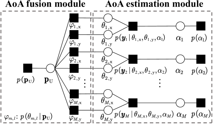
Figure 2: Factor graph representation of (III-B).

IV-A AoA Estimation Module

Before the message calculation, we present the pdf of the von Mises (VM) distribution of a random AoA $\theta$ as follows

$$\mathcal{M}\left(\pi\theta;\mu,\kappa\right)=\frac{1}{2\pi I_{0}\left(\kappa\right)}\exp\left(\kappa\cos\left(\pi\theta-\mu\right)\right),$$ (11)

where $\theta$ is scaled by constant $\pi$ to meet the standard expression of a VM distribution. In (11), $I_{0}$, $\mu$, and $\kappa$ represent the modified Bessel function of the first kind and order $0$, the mean direction parameter, and the concentration parameter, respectively.

We now consider the message from the variable node $\theta_{m,\mathrm{x}}$ to the factor node $\varphi_{m,\mathrm{x}}$, i.e., $\Delta_{\theta_{m,\mathrm{x}}\rightarrow\varphi_{m,\mathrm{x}}}$. Following the sum-product rule, we have

$$\Delta_{\theta_{m,\mathrm{x}}\rightarrow\varphi_{m,\mathrm{x}}}$$

$$\!\!\propto\!\!\int_{\theta_{m,\mathrm{y}}}\!\int_{\alpha_{m}}\!\!p\left(\boldsymbol{y}_{m}|\theta_{m,\mathrm{x}},\theta_{m,\mathrm{y}},\alpha_{m}\right)p\left(\alpha_{m}\right){\Delta_{\varphi_{m,\mathrm{y}}\rightarrow\theta_{m,\mathrm{y}}}}.$$ (12)

By denoting the right-hand side of (12) by $\Delta_{m,\mathrm{x}}$ and treating $\Delta_{\varphi_{m,\mathrm{x}}\rightarrow\theta_{m,\mathrm{x}}}$ as the prior distribution of $\theta_{m,\mathrm{x}}$, $\Delta_{\theta_{m,\mathrm{x}}\rightarrow\varphi_{m,\mathrm{x}}}$ can be further expressed as

$$\Delta_{\theta_{m,\mathrm{x}}\rightarrow\varphi_{m,\mathrm{x}}} \propto\frac{\Delta_{m,\mathrm{x}}\Delta_{\varphi_{m,\mathrm{x}}\rightarrow\theta_{m,\mathrm{x}}}}{\Delta_{\varphi_{m,\mathrm{x}}\rightarrow\theta_{m,\mathrm{x}}}},$$ (13a)

$$\propto\frac{p\left(\theta_{m,\mathrm{x}}|\boldsymbol{y}_{m}\right)}{\Delta_{\varphi_{m,\mathrm{x}}\rightarrow\theta_{m,\mathrm{x}}}},$$ (13b)

where (13b) follows by the Bayes’ theorem. The computation of $\Delta_{\theta_{m,\mathrm{x}}\rightarrow\varphi_{m,\mathrm{x}}}$ can be taken as a Bayesian line spectra estimation problem according to (13b). We assume that $\Delta_{\varphi_{m,\mathrm{x}}\rightarrow\theta_{m,\mathrm{x}}}$ is a VM distribution $\mathcal{M}\left(\pi\theta_{m,\mathrm{x}};\mu_{\varphi_{m,\mathrm{x}}\rightarrow\theta_{m,\mathrm{x}}},\kappa_{\varphi_{m,\mathrm{x}}\rightarrow\theta_{m,\mathrm{x}}}\right)$. The MVALSE algorithm proposed in [16] can be employed to obtain the estimated channel gain $\hat{\alpha}_{m}$ and the posterior estimate of $\theta_{m,\mathrm{x}}$ as $p\left(\theta_{m,\mathrm{x}}|\boldsymbol{y}_{m}\right)=\mathcal{M}\left(\pi\theta_{m,\mathrm{x}};\mu_{\theta_{m,\mathrm{x}}},\kappa_{\theta_{m,\mathrm{x}}}\right)$. Due to the closure of the VM distribution under multiplication, we have

$$\Delta_{\theta_{m,\mathrm{x}}\rightarrow\varphi_{m,\mathrm{x}}} \!\propto\frac{\mathcal{M}\left(\!\pi\theta_{m,\mathrm{x}};\mu_{\theta_{m,\mathrm{x}}},\kappa_{\theta_{m,\mathrm{x}}}\!\right)}{\mathcal{M}\left(\!\pi\theta_{m,\mathrm{x}};\mu_{\varphi_{m,\mathrm{x}}\rightarrow\theta_{m,\mathrm{x}}},\kappa_{\varphi_{m,\mathrm{x}}\rightarrow\theta_{m,\mathrm{x}}}\!\right)}$$ (14a)

$$\propto\!{\mathcal{M}\left(\!\pi\theta_{m,\mathrm{x}};\mu_{\theta_{m,\mathrm{x}}\rightarrow\varphi_{m,\mathrm{x}}},\kappa_{\theta_{m,\mathrm{x}}\rightarrow\varphi_{m,\mathrm{x}}}\!\right)},$$ (14b)

where $\mu_{\theta_{m,\mathrm{x}}\rightarrow\varphi_{m,\mathrm{x}}}$ and $\kappa_{\theta_{m,\mathrm{x}}\rightarrow\varphi_{m,\mathrm{x}}}$ satisfy

$$\kappa_{\theta_{m,\mathrm{x}}\rightarrow\varphi_{m,\mathrm{x}}}\exp{\left(j\mu_{\theta_{m,\mathrm{x}}\rightarrow\varphi_{m,\mathrm{x}}}\right)}$$

$$=\!\kappa_{\theta_{m,\mathrm{x}}}\!\exp{\left(j\mu_{\theta_{m,\mathrm{x}}}\!\right)}\!-\!\kappa_{\varphi_{m,\mathrm{x}}\rightarrow\theta_{m,\mathrm{x}}}\!\exp{\left(j\mu_{\varphi_{m,\mathrm{x}}\rightarrow\theta_{m,\mathrm{x}}}\!\right)}.$$ (15)

The message $\Delta_{\theta_{m,\mathrm{y}}\rightarrow\varphi_{m,\mathrm{y}}}$ can be obtained by replacing the subscript $\mathrm{x}$ with the subscript $\mathrm{y}$ in (14b), and (IV-A).

IV-B AoA Fusion Module

Given $p\left(\theta_{{m,l}}|\mathbf{p}_{\mathrm{U}}\right)$ in (8) and $\Delta_{\theta_{{m,l}}\rightarrow\varphi_{m,l}}$ in (14b), the message from $\varphi_{m,l}$ to $\mathbf{p}_{\mathrm{U}}$ can be expressed as

$$\Delta_{\varphi_{m,l}\rightarrow\mathbf{p}_{\mathrm{U}}}\propto\int_{\theta_{{m,l}}}{p\left(\theta_{{m,l}}|\mathbf{p}_{\mathrm{U}}\right)\Delta_{\theta_{{m,l}}\rightarrow\varphi_{m,l}}}$$ (16a)

$$\propto{\mathcal{M}\!\left(\!\frac{\pi\left(\mathbf{p}_{\mathrm{BS},m}\!-\!\mathbf{p}_{\mathrm{U}}\right)^{\mathrm{T}}\mathbf{e}_{l}}{\left\|\mathbf{p}_{\mathrm{BS},m}\!-\!\mathbf{p}_{\mathrm{U}}\right\|};\mu_{\theta_{{m,l}}\rightarrow\varphi_{m,l}},\kappa_{\theta_{{m,l}}\rightarrow\varphi_{m,l}}\!\!\right)}.$$ (16b)

Define $\mathcal{A}\triangleq\{(u,v)|1\leq u\leq M,v\in\{\mathrm{x},\mathrm{y}\}\}$. The message from $\mathbf{p}_{\mathrm{U}}$ to $\varphi_{m,l}$ is computed as

$$\Delta_{\mathbf{p}_{\mathrm{U}}\rightarrow\varphi_{m,l}}\propto p\left(\mathbf{p}_{\mathrm{U}}\right)\prod_{(n,k)\in\mathcal{A}\setminus(m,l)}{\Delta_{\varphi_{n,k}\rightarrow\mathbf{p}_{\mathrm{U}}}}$$ (17a)

$$\propto\prod_{(n,k)\in\mathcal{A}\setminus(m,l)}{\Delta_{\varphi_{n,k}\rightarrow\mathbf{p}_{\mathrm{U}}}}$$ (17b)

$$\!\propto\!\exp{\left\{\!\sum_{(n,k)\in\mathcal{A}\setminus(m,l)}{\kappa_{\theta_{n,k}\rightarrow\varphi_{n,k}}\cos\left(\theta_{n,k}\!-\!\mu_{\theta_{n,k}\rightarrow\varphi_{n,k}}\right)}\!\right\}},$$ (17c)

where (17b) holds by considering the non-informative Gaussian prior $p\left(\mathbf{p}_{\mathrm{U}}\right)$, and (17c) is due to (16b) with $\theta_{n,k}=\frac{\left(\mathbf{p}_{\mathrm{BS},n}-\mathbf{p}_{\mathrm{U}}\right)^{\mathrm{T}}\mathbf{e}_{k}}{\left\|\mathbf{p}_{\mathrm{BS},n}-\mathbf{p}_{\mathrm{U}}\right\|}$. To simplify message updates, (17c) is approximated as the following Gaussian pdf

$$\Delta_{\mathbf{p}_{\mathrm{U}}\rightarrow\varphi_{m,l}}\propto\mathcal{N}\left(\mathbf{p}_{\mathrm{U}};\mathbf{m}_{\mathbf{p}_{\mathrm{U}}\rightarrow\varphi_{m,l}},\mathbf{C}_{\mathbf{p}_{\mathrm{U}}\rightarrow\varphi_{m,l}}\right).$$ (18)

Note that the mean $\mathbf{m}_{\mathbf{p}_{\mathrm{U}}\rightarrow\varphi_{m,l}}$ and covariance $\mathbf{C}_{\mathbf{p}_{\mathrm{U}}\rightarrow\varphi_{m,l}}$ cannot be obtained by using moment matching since it is intractable to compute the first and second moments of (17c). Thus, we take the following method to obtain $\mathbf{m}_{\mathbf{p}_{\mathrm{U}}\rightarrow\varphi_{m,l}}$ and $\mathbf{C}_{\mathbf{p}_{\mathrm{U}}\rightarrow\varphi_{m,l}}$. Specifically, we use the gradient ascend method to solve the following optimization problem$\colon$

$$\hat{\mathbf{p}}_{\mathrm{U},(m,l)}=\arg\max_{\mathbf{p}_{\mathrm{U}}}\ h_{m,l}\left(\mathbf{p}_{\mathrm{U}}\right),$$ (19)

where $h_{m,l}\left(\cdot\right)$ denotes the exponential function of (17c) and $\hat{\mathbf{p}}_{\mathrm{U},(m,l)}$ is the local maximum of $h_{m,l}\left(\mathbf{p}_{\mathrm{U}}\right)$ given by gradient ascent. Then, $\mathbf{m}_{\mathbf{p}_{\mathrm{U}}\rightarrow\varphi_{m,l}}$ and $\mathbf{C}_{\mathbf{p}_{\mathrm{U}}\rightarrow\varphi_{m,l}}$ are approximated respectively as

$$\mathbf{m}_{\mathbf{p}_{\mathrm{U}}\rightarrow\varphi_{m,l}} =\hat{\mathbf{p}}_{\mathrm{U},(m,l)},$$ (20a)

$$\mathbf{C}_{\mathbf{p}_{\mathrm{U}}\rightarrow\varphi_{m,l}} =\left(\left.-\mathbf{H}\left(\mathbf{p}_{\mathrm{U}}\right)\right|_{\mathbf{p}_{\mathrm{U}}=\hat{\mathbf{p}}_{\mathrm{U},(m,l)}}\right)^{-1},$$ (20b)

where $\mathbf{H}\left(\mathbf{p}_{\mathrm{U}}\right)$ is the Hessian matrix of $h_{m,l}\left(\mathbf{p}_{\mathrm{U}}\right)$.

We now consider the message from $\varphi_{m,l}$ to $\theta_{m,l}$. Let $\bar{\mathbf{u}}_{m,l}=\mathbf{p}_{\mathrm{BS},m}-\mathbf{m}_{\mathbf{p}_{\mathrm{U}}\rightarrow\varphi_{m,l}}$. The unit vector perpendicular to $\bar{\mathbf{u}}_{m,l}$ within the plane spanned by $\bar{\mathbf{u}}_{m,l}$ and $\mathbf{e}_{l}$ is denoted by $\mathbf{v}_{m,l}=\frac{\left(\bar{\mathbf{u}}_{m,l}\times\mathbf{e}_{l}\right)\times\bar{\mathbf{u}}_{m,l}}{\left\|\left(\bar{\mathbf{u}}_{m,l}\times\mathbf{e}_{l}\right)\times\bar{\mathbf{u}}_{m,l}\right\|}$, where $\times$ represents the cross product here. We compute the message from $\varphi_{m,l}$ to $\theta_{m,l}$ as

$$\Delta_{\varphi_{m,l}\rightarrow\theta_{m,l}}\propto\int_{\mathbf{p}_{\mathrm{U}}}{p\left(\theta_{{m,l}}|\mathbf{p}_{\mathrm{U}}\right)\Delta_{\mathbf{p}_{\mathrm{U}}\rightarrow\varphi_{m,l}}}.$$ (21)

The integral in (21) has no closed-form expression. To simplify the calculation, we focus solely on the impact of the projection of the user location error on $\mathbf{v}_{m,l}$. The projection is denoted by a random variable $x_{m,l}$ with $x_{m,l}=\mathbf{v}_{m,l}^{\mathrm{T}}\left(\mathbf{p}_{\mathrm{U}}-\mathbf{m}_{\mathbf{p}_{\mathrm{U}}\rightarrow\varphi_{m,l}}\right)\mathbf{v}_{m,l}$. From (18), we have $p\left(x_{m,l}\right)=\mathcal{N}\left(0,\mathbf{v}_{m,l}^{\mathrm{T}}\mathbf{C}_{\mathbf{p}_{\mathrm{U}}\rightarrow\varphi_{m,l}}\mathbf{v}_{m,l}\right)$. The geometric constraint of $\theta_{{m,l}}$ and $x_{m,l}$ is denoted by $p\left(\theta_{{m,l}}|x\right)=\delta\left(x-\left\|\bar{\mathbf{u}}_{m,l}\right\|\tan\left(\arccos{\bar{\theta}_{m,l}}-\arccos{\theta_{m,l}}\right)\right)$ for a sufficiently large $\left\|\bar{\mathbf{u}}_{m,l}\right\|$ under Assumption 1. Then, $\Delta_{\varphi_{m,l}\rightarrow\theta_{m,l}}$ is reduced to

$$\Delta_{\varphi_{m,l}\rightarrow\theta_{m,l}}\propto\int_{x_{m,l}}{p\left(\theta_{{m,l}}|x_{m,l})p(x_{m,l}\right)}$$ (22a)

$$\propto\exp\left(\!-\frac{\left\|\bar{\mathbf{u}}_{m,l}\right\|^{2}\tan^{2}\left(\arccos{\bar{\theta}}_{m,l}\!-\!\arccos{\theta_{m,l}}\right)}{2\mathbf{v}_{m,l}^{\mathrm{T}}\mathbf{C}_{\mathbf{p}_{\mathrm{U}}\rightarrow\varphi_{m,l}}\mathbf{v}_{m,l}}\!\right)$$ (22b)

$$\propto\mathcal{M}\left(\pi\theta_{m,l};\mu_{\varphi_{m,l}\rightarrow\theta_{m,l}},\kappa_{\varphi_{m,l}\rightarrow\theta_{m,l}}\right),$$ (22c)

where (22c) holds by approximating (22b) as a VM distribution. In (22c),

$$\mu_{\varphi_{m,l}\rightarrow\theta_{m,l}} =\pi\bar{\theta}_{m,l},$$ (23a)

$$\kappa_{\varphi_{m,l}\rightarrow\theta_{m,l}} =\frac{\left\|\bar{\mathbf{u}}_{m,l}\right\|^{2}}{\pi^{2}\left(1-\bar{\theta}_{m,l}^{2}\right)\mathbf{v}_{m,l}^{\mathrm{T}}\mathbf{C}_{\mathbf{p}_{\mathrm{U}}\rightarrow\varphi_{m,l}}\mathbf{v}_{m,l}},$$ (23b)

where $\bar{\theta}_{m,l}$ is the maximum point of (22b), and (23b) follows by equating (22b) and (22c) based on Taylor series expansion at $\bar{\theta}_{m,l}$.

Input: $n_{1}$, $n_{2}$, $\sigma^{2}$, $f$, $d_{\mathrm{x}}$, $d_{\mathrm{y}}$, $N_{\mathrm{x}}$, $N_{\mathrm{y}}$, $M$, $\mathbf{p}_{\mathrm{BS}}$, and $\boldsymbol{y}$.

Output: User location estimation.

1:  repeat

2:     % AoA estimation module

3:     for $m=1$ to $M$ do

4:         $\forall{l\in\{\mathrm{x},\mathrm{y}\}}$, update $p\left(\theta_{m,l}|\boldsymbol{y}_{m}\right)$ and $\hat{\alpha}_{m}$ by the MVALSE algorithm.

5:         $\forall{l\in\{\mathrm{x},\mathrm{y}\}}$, update $\Delta_{\theta_{m,l}\rightarrow\varphi_{m,l}}\left(\theta_{m,l}\right)$ by following (14b), (IV-A).

6:     end for

7:     % AoA fusion module

8:     for $m=1$ to $M$ do

9:         $\forall{l\in\{\mathrm{x},\mathrm{y}\}}$, update $\Delta_{\varphi_{m,l}\rightarrow\mathbf{p}_{\mathrm{U}}}$ by (16b).

10:         $\forall{l\in\{\mathrm{x},\mathrm{y}\}}$, update $\hat{\mathbf{p}}_{\mathrm{U},(m,l)}$ by solving the optimization problem in (19) via gradient ascent method.

11:         $\forall{l\in\{\mathrm{x},\mathrm{y}\}}$, update $\Delta_{\mathbf{p}_{\mathrm{U}}\rightarrow\varphi_{m,l}}$ by (20a), (20b).

12:         $\forall{l\in\{\mathrm{x},\mathrm{y}\}}$, update $\Delta_{\varphi_{m,l}\rightarrow\theta_{m,l}}$ by (22c),(23a),(23b).

13:     end for

14:  until the maximum number of iterations $n_{1}$ is reached.

15:  return

Algorithm 1 APLE Algorithm

IV-C Overall Algorithm

The APLE algorithm is summarized in Algorithm 1. The messages are iteratively passed between the AoA estimation and AoA fusion modules until the maximum number of iterations $n_{1}$ is reached. The complexity of the APLE algorithm primarily arises from the AoA estimation module. The complexity of calculating $p\left(\theta_{m,\mathrm{x}}|\boldsymbol{y}_{m}\right)$ and $p\left(\theta_{m,\mathrm{y}}|\boldsymbol{y}_{m}\right)$ is $\mathcal{O}\left(n_{2}N_{m,\mathrm{x}}N_{m,\mathrm{y}}\right)$ where $n_{2}$ is the number of iterations in MVALSE. Therefore, the overall complexity of APLE is $\mathcal{O}\left(n_{1}n_{2}N_{\mathrm{B}}\right)$ by noting $N_{\mathrm{B}}=MN_{m,\mathrm{x}}N_{m,\mathrm{y}}$.

V Numerical Results

In this section, we numerically evaluate the performance of the proposed APLE algorithm. For comparison, we introduce two baselines. For the first baseline, we extend the OMP algorithm in [17] to the three-dimensional case, with grid search accuracies of $0.1$m for $r$ and $0.02^{\circ}$ for $\omega$ and $\phi$. The extended algorithm is referred to as “OMP”. For the second baseline, we simplify the MUSIC algorithm by constructing new covariance matrixes that decouple the angle and distance parameters following the method outlined in [12]. The resulting algorithm is referred to as “MUSIC”. To accommodate the model mismatch introduced by Assumption 1, we follow the MCRB analysis[13] to yield a performance LB of the APLE algorithm. We set $N_{\mathrm{x}}=N_{\mathrm{y}}$ and $N_{m,\mathrm{x}}=N_{m,\mathrm{y}}$, for $1\leq m\leq M$. The experiments are conducted on a Windows x64 computer with a 3 GHz CPU and 64 GB RAM.

Fig. 3 illustrates the normalized mean squared error (NMSE) for location estimation against SNR at various user-to-BS-array distances $r$. In Fig. 3, we set $d=\frac{\lambda}{4}$ since the MUSIC algorithm is limited to $d\leq\frac{\lambda}{4}$. We further set $f=28$GHz, $\lambda=0.0107$m, $N_{\mathrm{x}}=30$, $N_{m,\mathrm{x}}=10$, and $M=9$, resulting in $R_{\mathrm{F}}=2.4107$m and $R_{m,\mathrm{F}}=0.2679$m. We consider a relatively small $N_{\mathrm{x}}$ for ease of running the simulations of the baseline algorithms. We choose $r=R_{m,\mathrm{F}}$ and $r=R_{\mathrm{F}}$ to show the algorithm performance at near/far-field boundaries of the subarray and the BS array, respectively. On the left plot of Fig. 3, APLE outperforms the baselines significantly at $r=R_{m,\mathrm{F}}$, which demonstrates the superior localization accuracy of the proposed algorithm. On the right plot of Fig. 3, APLE performs close to MUSIC at $r=R_{\mathrm{F}}$, but as shown later, APLE runs much faster than MUSIC.

Fig. 4 shows the impact of AoA drifting on the NMSE performance of APLE for different $N_{\mathrm{x}}$, $M$, and $r$. We set SNR $=20$dB and $d=\frac{\lambda}{2}$. $N_{\mathrm{x}}$ is set to $60$, $120$, and $180$. As seen from Fig. 4, as the increases of $M$ and $r$, the NMSE becomes worse. This is because the increases of $M$ and $r$ both weaken the AoA drifting effect across different subarrays. We see that the APLE algorithm can closely approach the LB.

Table I demonstrates the impact of increasing the number of BS antennas on runtime and NMSE. We set SNR $=20$dB, $d=\frac{\lambda}{4}$, and $r=2$m. $N_{\mathrm{x}}$ is set to $30$, $50$, $75$, and $100$ with the corresponding $N_{m,\mathrm{x}}$ being $15$, $25$, $25$, and $25$. In Table I, for $N_{\mathrm{x}}\times N_{\mathrm{y}}=100\times 100$, both the OMP and MUSIC algorithms run out of memory. We see that APLE consistently achieves reduced NMSE with nearly linear growth in runtime as the number of BS antennas increases, highlighting remarkable scalability for its implementation in large-scale antenna arrays.

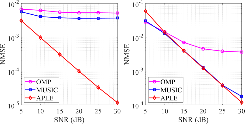
Figure 3: The NMSE of the APLE algorithm and its baselines v.s. SNR, where $r=R_{m,\mathrm{F}}=0.2679$m on the left plot and $r=R_{\mathrm{F}}=2.4107$m on the right plot.

TABLE I: The runtime and NMSE of the APLE algorithm and its baselines with various $N_{\mathrm{x}}$.

	Runtime (s)			NMSE (dB)
$N_{\mathrm{x}}\times N_{\mathrm{y}}$	APLE	MUSIC	OMP	APLE	MUSIC	OMP
$30\times 30$	0.0078	0.1039	4.3827	-29.70	-30.13	-22.12
$50\times 50$	0.0184	0.9073	11.2291	-43.85	-40.06	-22.37
$75\times 75$	0.0400	15.6617	32.5967	-51.18	-40.10	-22.43
$100\times 100$	0.0700	-	-	-55.47	-	-

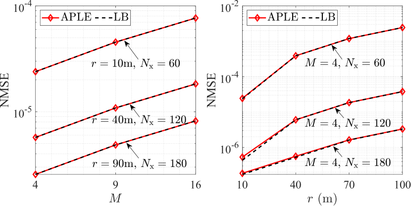
Figure 4: The NMSE of the APLE algorithm and the LB for different $N_{\mathrm{x}}$ with various $M$ and $r$.

VI Conclusion

In this paper, we proposed the APLE algorithm to solve the 3D near-field user location estimation problem in the ELAA system. By partitioning the BS array, the far-field assumption holds for each subarray. We established a probabilistic model for user location estimation by leveraging the geometric correlation between the AoA at each subarray and the user’s location. Additionally, we introduced a low-complexity scalable user location estimation algorithm based on the message-passing principle. Simulation results demonstrated that the APLE algorithm achieves remarkable localization accuracy and exhibits excellent scalability as the array size goes large.

References

- [1] Z. Xiao and Y. Zeng, “An overview on integrated localization and communication towards 6G,” Sci. China Inf. Sci., vol. 65, no. 3, pp. 1–46, Mar. 2022.
- [2] H. Viswanathan and P. E. Mogensen, “Communications in the 6G era,” IEEE Access, vol. 8, pp. 57 063–57 074, 2020.
- [3] B. Teng, X. Yuan, R. Wang, and S. Jin, “Bayesian user localization and tracking for reconfigurable intelligent surface aided MIMO systems,” IEEE J. Sel. Areas Commun., vol. 16, no. 5, pp. 1040–1054, Aug. 2022.
- [4] S. Guo and K. Qu, “Beamspace modulation for near field capacity improvement in XL-MIMO communications,” IEEE Wireless Commun. Lett., vol. 12, no. 8, pp. 1434–1438, Aug. 2023.
- [5] K. Qu, S. Guo, and N. Saeed, “Near-field integrated sensing and communication: Performance analysis and beamforming design,” arXiv preprint arXiv:2308.06455, Aug. 2023.
- [6] M. Cui, Z. Wu, Y. Lu, X. Wei, and L. Dai, “Near-field MIMO communications for 6G: Fundamentals, challenges, potentials, and future directions,” IEEE Commun. Mag., vol. 61, no. 1, pp. 40–46, Jan. 2023.
- [7] E. Björnson, L. Sanguinetti, H. Wymeersch, J. Hoydis, and T. L. Marzetta, “Massive MIMO is a reality—What is next?: Five promising research directions for antenna arrays,” Digit. Signal Process., vol. 94, pp. 3–20, Nov. 2019.
- [8] D. Dardari, N. Decarli, A. Guerra, and F. Guidi, “LOS/NLOS near-field localization with a large reconfigurable intelligent surface,” IEEE Trans. Wireless Commun., vol. 21, no. 6, pp. 4282–4294, Jun. 2022.
- [9] G. Wang and K. C. Ho, “Convex relaxation methods for unified near-field and far-field TDOA-based localization,” IEEE Trans. Wireless Commun., vol. 18, no. 4, pp. 2346–2360, Apr. 2019.
- [10] J. Liang and D. Liu, “Passive localization of mixed near-field and far-field sources using two-stage MUSIC algorithm,” IEEE Trans. Signal Process., vol. 58, no. 1, pp. 108–120, Jan. 2010.
- [11] X. Su, Z. Liu, B. Sun, Y. Wang, X. Chen, and X. Li, “Fast BSC-based algorithm for near-field signal localization via uniform circular array,” J. Syst. Eng. Electron., vol. 33, no. 2, pp. 269–278, Apr. 2022.
- [12] O. Rinchi, A. Elzanaty, and M.-S. Alouini, “Compressive near-field localization for multipath RIS-aided environments,” IEEE Commun. Lett., vol. 26, no. 6, pp. 1268–1272, Jun. 2022.
- [13] H. Chen et al., “Channel model mismatch analysis for XL-MIMO systems from a localization perspective,” Proc. IEEE GLOBECOM, pp. 1588–1593, Dec. 2022.
- [14] K. T. Selvan and R. Janaswamy, “Fraunhofer and Fresnel distances: Unified derivation for aperture antennas,” IEEE Antennas Propag. Mag., vol. 59, no. 4, pp. 12–15, Aug. 2017.
- [15] M. Zhang and X. Yuan, “Intelligent reflecting surface aided MIMO with cascaded LoS links: Channel modelling and full multiplexing region,” IEEE Trans. Wireless Commun., 2023, doi:10.1109/TWC.2023.3287040.
- [16] Q. Zhang, J. Zhu, N. Zhang, and Z. Xu, “Multidimensional variational line spectra estimation,” IEEE Signal Process. Lett., vol. 27, pp. 945–949, 2020.
- [17] X. Wei and L. Dai, “Channel estimation for extremely large-scale massive MIMO: Far-field, near-field, or hybrid-field?” IEEE Commun. Lett., vol. 26, no. 1, pp. 177–181, Jan. 2022.