Engineering an Exact Pseudo-Boolean Model Counter

Abstract

Model counting, a fundamental task in computer science, involves determining the number of satisfying assignments to a Boolean formula, typically represented in conjunctive normal form (CNF). While model counting for CNF formulas has received extensive attention with a broad range of applications, the study of model counting for Pseudo-Boolean (PB) formulas has been relatively overlooked. Pseudo-Boolean formulas, being more succinct than propositional Boolean formulas, offer greater flexibility in representing real-world problems. Consequently, there is a crucial need to investigate efficient techniques for model counting for PB formulas.

In this work, we propose the first exact Pseudo-Boolean model counter, $\mathsf{PBCount}$, that relies on knowledge compilation approach via algebraic decision diagrams. Our extensive empirical evaluation shows that $\mathsf{PBCount}$ can compute counts for 1513 instances while the current state-of-the-art approach could only handle 1013 instances. Our work opens up several avenues for future work in the context of model counting for PB formulas, such as the development of preprocessing techniques and exploration of approaches other than knowledge compilation.

1 Introduction

Propositional model counting involves computing the number of satisfying assignments to a Boolean formula. Model counting is closely related to the Boolean satisfiability problem where the task is to determine if there exists an assignment of variables such that the Boolean formula evaluates to true. Boolean satisfiability and model counting have been extensively studied in the past decades and are the cornerstone of an extensive range of real-life applications such as software design, explainable machine learning, planning, and probabilistic reasoning (Bacchus, Dalmao, and Pitassi 2003; Narodytska et al. 2019; Jackson 2019; Fan, Miller, and Mitra 2020). Owing to decades of research, there are numerous tools and techniques developed for various aspects of Boolean satisfiability and model counting, from Boolean formula preprocessors to SAT solvers and model counters.

The dominant representation format of Boolean formulas is Conjunctive Normal Form (CNF), and accordingly, the tools in the early days focused on CNF as the input format. Over the past decade and a half, there has been considerable effort in exploring other representation formats: one such format that has gained significant interest from the community is Pseudo-Boolean (PB) formulas, which are expressed as the conjunction of linear inequalities. PB formulas are shown to be more succinct than CNF formulas and natural for problems such as Knapsack, sensor placement, binarized neural networks, and the like. Furthermore, PB formulas are able to express constraints more succinctly compared to Boolean formulas in CNF (Berre et al. 2018). As an example, a single PB constraint is sufficient to express at-most-$k$ and at-least-$k$ types of cardinal constraints whereas the equivalent in CNF would require a polynomial number of clauses (Sinz 2005). On a higher level, an arbitrary CNF clause can be expressed with a single PB constraint but the converse is not true (Berre et al. 2018). The past decade has witnessed the development of satisfiability solving techniques based on the underlying proof systems naturally suited to PB constraints, and accordingly, the state-of-the-art PB solvers, such as $\mathsf{RoundingSat}$ significantly outperform CNF solvers on problems that are naturally encoded in PB (Elffers and Nordström 2018; Devriendt 2020; Devriendt et al. 2021).

In contrast to satisfiability, almost all the work in the context of model counting has focused on the representation of Boolean formulas in Conjunctive Normal Form (CNF), with the sole exception of the development of an approximate model counter for PB formulas (Yang and Meel 2021).

The primary contribution of this work is to address the aforementioned gap through the development of a native scalable exact model counter, called $\mathsf{PBCount}$, for PB formulas. $\mathsf{PBCount}$ is based on the knowledge compilation paradigm, and in particular, compiles a given PB formula into algebraic decision diagrams (ADDs) (Bahar et al. 1993), which allows us to perform model counting. We perform extensive empirical evaluations on benchmark instances arising from different applications, such as sensor placement, multi-dimension knapsack, and combinatorial auction benchmarks (Gens and Levner 1980; Blumrosen and Nisan 2007; Latour, Sen, and Meel 2023). Our evaluations highlighted the efficacy of $\mathsf{PBCount}$ against existing state-of-the-art CNF model counters. In particular, $\mathsf{PBCount}$ is able to successfully count 1513 instances while the prior state of the art could only count 1013 instances, thereby demonstrating significant runtime improvements. It is worth remarking that $\mathsf{PBCount}$ achieves superior performance with substantially weaker preprocessing techniques in comparison to techniques employed in CNF model counters, making a strong case for the advantages of native PB model counting and reasoning. Furthermore, given the crucial importance of preprocessing techniques for CNF counting, we hope our work will motivate the development of preprocessing techniques for PB model counting.

The rest of the paper is organized as follows: We discuss the preliminaries and existing counting algorithm in Section 2. In Section 3, we discuss existing works and how they relate to our approach, which we detail in Section 4. Following that, we analyze the empirical results of $\mathsf{PBCount}$ against existing tools in Section 5 and conclude in Section 6.

2 Preliminaries

Boolean Formula

A Boolean variable can take values true or false. A literal is either a Boolean variable or its negation. Let $F$ be a Boolean formula. $F$ is in conjunctive normal form (CNF) if $F$ is a conjunction of clauses, where each clause is a disjunction of literals. $F$ is satisfiable if there exists an assignment $\tau$ of variables of $F$ such that $F$ evaluates to true. We refer to $\tau$ as a satisfying assignment of $F$ and denote the set of all $\tau$ as $\mathsf{Sol}(F)$. Model counting for Boolean formula $F$ refers to the task of determining $|\mathsf{Sol}(F)|$.

Pseudo-Boolean Formula

A PB constraint is either an equality or inequality of the form $\sum_{i=1}^{n}a_{i}x_{i}\square k$ where $x_{1},...,x_{n}$ are Boolean literals, $a_{1},...,a_{n}$, and $k$ are integers, and $\square$ is one of $\{\geq,=,\leq\}$. We refer to $a_{1},...,a_{n}$ as term coefficients in the PB constraint, where each term is of the form $a_{i}x_{i}$. A PB formula, $G$, consists of a set of PB constraints. $G$ is satisfiable if there exists an assignment $\tau$ of all variables of $G$ such that all its PB constraints hold. PB model counting refers to the computation of $|\mathsf{Sol}(G)|$ where $\mathsf{Sol}(G)$ is the set of all satisfying assignments of $G$.

Projected Model Counting

Let $G$ be a formula defined over the set of variables $X$. Let $V_{i},V_{j}$ be subsets of $X$ such that $V_{i}\cap V_{j}=\emptyset$ and $V_{i}\cup V_{j}=X$. Projected model counting of $G$ on $V_{i}$ refers to the number of assignments of all variables in $V_{i}$ such that there exists an assignment of variables in $V_{j}$ that makes $G$ evaluate to true (Aziz et al. 2015). In the evaluations, CNF model counter baselines perform projected model counting on the original variables in the PB formula, to avoid additional counts due to auxiliary variables introduced in the PB to CNF conversion process.

Algebraic Decision Diagram

An algebraic decision diagram (ADD) is a directed acyclic graph representation of a function $f:2^{X}\rightarrow S$ where $X$ is the set of Boolean variables that $f$ is defined over, and $S$ is an arbitrary set known as the carrier set. We denote the function represented by an ADD $\psi$ as $\mathsf{Func}(\psi)$. The internal nodes of ADD represent decisions on variables $x\in X$ and the leaf nodes represent $s\in S$. In this work, we focus on the setting where $S\subset\mathbb{Z}$. As an example, an ADD representing $3x_{1}+4x_{2}$ is shown in Figure 1. In the figure, a dotted arrow from an internal node represents when the corresponding variable is set to false and a solid arrow represents when it is set to true.

Figure 1: An ADD representing $3x_{1}+4x_{2}$

In addition, we make use of $\mathsf{Apply}$ and $\mathsf{ITE}$ operations on ADDs (Bryant 1986; Bahar et al. 1993). The $\mathsf{Apply}$ operation takes as input a binary operator $\bowtie$, two ADDs $\psi_{1},\psi_{2}$, and outputs an ADD $\psi_{3}$ such that the $\mathsf{Func}(\psi_{3})=\mathsf{Func}(\psi_{1})\bowtie\mathsf{Func}(\psi_{2})$. The $\mathsf{ITE}$ operation (if-then-else) involves 3 ADDs $\psi_{1},\psi_{2},\psi_{3}$, where carrier set of $\psi_{1}$ is restricted to $\{0,1\}$. $\mathsf{ITE}$ outputs an ADD that is equivalent to having 1 valued leaf nodes in $\psi_{1}$ replaced with $\psi_{2}$ and 0 valued leaf nodes with $\psi_{3}$.

Relation of Pseudo-Boolean Constraint to CNF Clause

Given an arbitrary CNF clause $D$, one could always convert $D$ to a PB constraint. Given that $D$ is of the form $\bigvee_{i=1}^{m}l_{i}$, where $l_{1},...,l_{m}$ are Boolean literals, $D$ can be represented by a single PB constraint $\sum_{i=1}^{m}a_{i}l_{i}\geq 1$ where all coefficients $a_{1},...,a_{i},...a_{m}$ are $1$. However, there are PB constraints that require polynomially many CNF clauses to represent. An example would be $\sum_{i=1}^{m}l_{i}\geq k$ which requires at least $k$ of $m$ literals to be true. We refer the reader to the Appendix for statistics of the number of variables and clauses before and after PB to CNF conversion for benchmarks used.

2.1 Model Counting with ADDs

In this work, we adapt the existing dynamic programming counting algorithm of $\mathsf{ADDMC}$ (Dudek, Phan, and Vardi 2020a), shown in Algorithm 1, to perform PB model counting with ADDs. This includes using the default $\mathsf{ADDMC}$ configurations for ADD variable ordering (MCS) and cluster ordering $\rho$ (BOUQUET_TREE). The algorithm takes in a list $\varphi$ of ADDs, representing all constraints, and an order $\rho$ of which to process the ADDs. ADD $\psi$ is initialized with value $1$. According to cluster ordering $\rho$, cluster ADDs $\psi_{j}$ are formed using the $\mathsf{Apply}$ operation with $\times$ operator on each of the individual constraint ADDs of constraints in the cluster. The cluster ADD $\psi_{j}$ is combined with $\psi$ using the same $\mathsf{Apply}$ operation. If variable $x$ does not appear in later clusters in $\rho$, it is abstracted out from $\psi$ (early projection process in $\mathsf{ADDMC}$) using $\psi\leftarrow\mathcal{W}(\bar{x})\times\psi[x\mapsto 0]+\mathcal{W}(x)\times\psi[x\mapsto 1]$ in line 8, where $\mathcal{W}(\cdot)$ is the user provided literal weight function. In unweighted model counting, $\mathcal{W}(\cdot)$ is 1 for all literals. Once all clusters have been processed, the unprocessed variables $x$ of the formula $G$ are abstracted out using the same operation as before (line 10). After all variables are abstracted out, $\psi$ is a constant ADD that represents the final count.

Algorithm 1 computeCount($\varphi,\rho$)

Input: $\varphi$ - list of ADD, $\rho$ - cluster merge ordering

Output: model count

1:  $\psi\leftarrow\mathsf{constantADD}(1)$

2:  for $\mathsf{cluster}$ $A_{j}\in\rho$ do

3:     $\psi_{j}\leftarrow\mathsf{constantADD}(1)$

4:     for $\mathsf{constraint}$ $C_{i}\in A_{j}$ do

5:        $\psi_{j}\leftarrow\psi_{j}\times\varphi[C_{i}]$

6:     $\psi\leftarrow\psi\times\psi_{j}$

7:     for each $x\in\psi$ where $x$ not in later clusters in $\rho$ do

8:        $\psi\leftarrow\mathcal{W}(\bar{x})\times\psi[x\mapsto 0]+\mathcal{W}(x)\times\psi[x\mapsto 1]$

9:  for all unprocessed variable $x$ do

10:     $\psi\leftarrow\mathcal{W}(\bar{x})\times\psi[x\mapsto 0]+\mathcal{W}(x)\times\psi[x\mapsto 1]$

11:  return  $\mathsf{getValue}(\psi)$

3 Related Work

Boolean Formula Preprocessing

Boolean formula preprocessing involves simplifying a given formula to reduce runtimes of downstream tasks such as determining satisfiability of the formula (SAT-solving) and model counting. Preprocessing is crucial to modern SAT solvers and model counters’ performance improvements in recent decades. There are numerous preprocessing techniques introduced over the years by the research community, some of which are unit propagation, bounded variable elimination, failed literal probing, and vivification (Dowling and Gallier 1984; Berre 2001; Eén and Biere 2005; Piette, Hamadi, and Sais 2008). In this work, we adapt some of the SAT preprocessing techniques, namely unit propagation and a variant of failed literal probing, to simplify PB formulas.

Search-Based Model Counters

Among the numerous existing CNF model counters, we can classify them into two main categories – search-based model counters and decision diagram-based model counters. Notable existing search-based model counters include $\mathsf{GPMC}$, $\mathsf{Ganak}$, and Sharpsat-TD (Ryosuke Suzuki and Sakai 2017; Sharma et al. 2019; Korhonen and Järvisalo 2021). Search-based model counters work by setting values to variables in a given formula in an iterative manner, which is equivalent to implicitly exploring a search tree. In addition, search-based model counters adapt techniques such as sub-component caching from SAT solving for more efficient computation.

Decision Diagram-Based Model Counter

Decision diagram-based model counters employ knowledge compilation techniques to compile a given formula into directed acyclic graphs (DAGs) and perform model counting with these DAGs. Some of the recent decision diagram-based model counters are $\mathsf{D4}$, ExactMC, $\mathsf{ADDMC}$, and its related variant $\mathsf{DPMC}$ (Lagniez and Marquis 2017; Dudek, Phan, and Vardi 2020a, b; Lai, Meel, and Yap 2021). $\mathsf{D4}$ and ExactMC compile the formula in a top-down manner into the respective decision diagram forms. In contrast, $\mathsf{ADDMC}$ and $\mathsf{DPMC}$ (decision diagram mode) perform bottom-up compilations of algebraic decision diagrams (ADDs). In this work, we based $\mathsf{PBCount}$ on $\mathsf{ADDMC}$ and introduced techniques to compile a PB constraint directly into an ADD and employ the same counting approach in $\mathsf{ADDMC}$.

Pseudo-Boolean Conversion

One way to perform PB model counting is to convert the PB formula to a Boolean formula and use existing CNF model counters. A notable tool for the conversion of PB to CNF is $\mathsf{PBLib}$ (Philipp and Steinke 2015). $\mathsf{PBLib}$ implements various encodings to convert PB formulas into CNF form, some of which include cardinality networks, sorting networks, and BDD-based encodings (Eén and Sörensson 2006; Abío et al. 2011, 2013). In this work, we use default settings for the $\mathsf{PBEncoder}$ binary provided as part of $\mathsf{PBLib}$ to perform the required conversions. We subsequently compare $\mathsf{PBCount}$ against state-of-the-art CNF model counters. It is worth noting that the model counting task for PB formula becomes a projected model counting task of the corresponding CNF formula, as previously mentioned in Section 2.

4 Approach

We show the overall flow of $\mathsf{PBCount}$ in Figure 2. We first preprocess the PB formula using propagation and assumption probing. Subsequently, we compile each of the PB constraints into an algebraic decision diagram (ADD). Next, we merge constraint ADDs using $\mathsf{Apply}$ operation and perform model counting by abstracting out variables (Section 2.1). The model count would be the value after all variables are abstracted out. Without loss of generality, the algorithms described in this work handle PB constraints involving ‘$=$’ and ‘$\geq$’ operators, as ‘$\leq$’ type constraints can be manipulated into ‘$\geq$’ type constraints.

Figure 2: Overall flow of our PB model counter $\mathsf{PBCount}$. Shaded boxes indicate our contributions.

4.1 Preprocessing

Figure 3: Preprocessing of PB formula

The preprocessing phase of $\mathsf{PBCount}$ performs assumption probing and unit propagation (Biere, Järvisalo, and Kiesl 2021). $\mathsf{PBCount}$ repeatedly performs unit propagation and assumption probing until no change is detected, as shown in Algorithm 2.

Algorithm 2 Preprocess($G$)

Input: $G$ - PB formula

Output: $G^{\prime}$ - preprocessed PB formula

1:  mapping $\leftarrow$ []; $G^{\prime}\leftarrow G$

2:  repeat

3:     for all single variable constraint $C\in G^{\prime}$ do

4:        mapping $\leftarrow$ mapping $\cup$ $\mathsf{InferDecision}(C)$

5:     $G^{\prime}\leftarrow\mathsf{propagate}$($G^{\prime}$, mapping)

6:     for all variable $x\in G^{\prime}$ do

7:        mapping $\leftarrow$ mapping $\cup$ $\mathsf{AssumProbe}(G^{\prime},x)$

8:     $G^{\prime}\leftarrow\mathsf{propagate}$($G^{\prime}$, mapping)

9:  until $G^{\prime}$ does not change

10:  return  $G^{\prime}$

Sign Manipulation

Let $C$ be the PB constraint $-3x_{1}-4x_{2}\leq-3$. One can multiply both sides of the constraint by $-1$ to form $3x_{1}+4x_{2}\geq 3$. In addition, one would be able to switch the sign of the coefficient of $x_{2}$ as follows.

$$3x_{1}+4x_{2}\geq 3$$

$$3x_{1}+4(1-\bar{x}_{2})\geq 3$$

$$3x_{1}-4\bar{x}_{2}\geq-1$$

In general, one is able to manipulate the sign of any term coefficient as shown in the example above. We use the above technique to optimize PB constraint compilation approaches which we discuss in later sections.

Propagation

Propagation in the Pseudo-Boolean context refers to the simplification of the PB constraints if decisions on some PB variables can be inferred. In particular, one might be able to infer decisions on PB variable $x_{i}$ from PB constraint $C_{j}$ when the constraint is of either 1) $a_{i}x_{i}\geq k$ or 2) $a_{i}x_{i}=k$ forms. We defer the details of the $\mathsf{InferDecision}$ algorithm to the Appendix.

Algorithm 3 AssumProbe($G$, $x_{i}$)

Input: $G$ - PB formula, $x_{i}$ - assumption variable

Output: mapping of variable values

1:  temp, mapping $\leftarrow[]$

2:  for all constraint $C\in G[x_{i}\mapsto 1]$ do

3:     temp $\leftarrow$ temp $\cup$ $\mathsf{InferDecision(C)}$

4:  for all constraint $C\in G[x_{i}\mapsto 0]$ do

5:     temp $\leftarrow$ temp $\cup$ $\mathsf{InferDecision(C)}$

6:  for all variable $x_{j}$, where $j\not=i$ do

7:     if exactly one literal of $x_{j}$ in temp then

8:        mapping $\leftarrow$ mapping $\cup$ temp[$x_{j}$]

9:  return  mapping

Assumption Probing

Assumption probing can be viewed as a weaker form of failed literal probing (Biere, Järvisalo, and Kiesl 2021) as well as single step look ahead propagation process. For an arbitrary variable $x_{i}\in G$, where $G$ is the PB formula, assumption probing involves performing propagation and decision inference independently for when $x_{i}=0$ and $x_{i}=1$. If another variable $x_{j}$ is inferred to have the same value assignment $\tau[x_{j}]$ in both cases, then it can be inferred that $x_{j}$ should be set to $\tau[x_{j}]$ in all satisfying assignments of $G$. Algorithm 3 illustrates the process for a single variable $x_{i}$, and in the preprocessing stage, we perform assumption probing on all variables in $G$.

4.2 Pseudo-Boolean Constraint Compilation

In this work, we introduce two approaches, namely top-down and bottom-up, to compile each constraint of a PB formula into an ADD. We use $T,k,$ and $eq$ in place of PB constraint $C$ when describing the compilation algorithms. $T$ refers to the term list, which is a list of $a_{i}x_{i}$ terms of $C$. $k$ is the constraint constant and $eq$ indicates if $C$ is ‘=’ constraint.

Figure 4: An ADD $\psi_{1}$ representing $3x_{1}+4x_{2}\geq 3$

Bottom-up ADD Constraint Compilation

In order to compile an ADD which represents a PB constraint of the following form $\sum_{i=1}^{n}a_{i}x_{i}[\geq,=,\leq]k$, we first start compiling the expression $\sum_{i=1}^{n}a_{i}x_{i}$ from literal and constant ADDs as shown by line 3 of Algorithm 4. A constant ADD which represents integer $a_{i}$ is a single leaf node that has value $a_{i}$. A literal ADD comprises of an internal node, which represents variable $x$, and true and false leaf nodes, which represent the evaluated values of the literal if $x$ is set to true and false. With the literal and constant ADDs, we use $\mathsf{Apply}$ with $\times$ operator to form ADDs for each term $a_{i}x_{i}$. We use $\mathsf{Apply}$ with $+$ operator on term ADDs to form the ADD representing expression $\sum_{i=1}^{n}a_{i}x_{i}$. As an example, the ADD $\psi$ for the expression $3x_{1}+4x_{2}$ is shown in Figure 1. To account for the inequality or equality, we look at the value of leaf nodes in expression ADD $\psi$ and determine if they satisfy the constraint (lines 4 to 10). We replace the leaf nodes with $1$ node if the constraint is satisfied and $0$ node otherwise, the resultant ADD is illustrated in Figure 4.

Algorithm 4 compileConstraintBottomUp($T,k,eq$)

Input: $T$ - term list, $k$ - constraint value,

$eq$ - indicator if constraint is ‘=’ type

Output: $\psi$ - constraint ADD

1:  $\psi\leftarrow\mathsf{constantADD}(0)$

2:  for term $t$ in $T$ do

3:     $\psi\mathrel{+}=\mathsf{constantADD}$(t.coeff) $\mathrel{\times}\mathsf{literalADD}$(t.literal)

4:  for node $n$ in $\mathsf{LeafNode}(\psi)$ do

5:     if $eq$ is true & $n$.value $=k$ then

6:        $n$.value $\leftarrow$ 1

7:     else if $eq$ is false & $n$.value $\geq k$ then

8:        $n$.value $\leftarrow$ 1

9:     else

10:        $n$.value $\leftarrow$ 0

11:  return  $\psi$

Top-down ADD Constraint Compilation

In contrast to the bottom-up ADD compilation approach, the top-down ADD compilation for a given PB constraint involves the if-then-else ($\mathsf{ITE}$) operation for decision diagrams. We only consider PB constraints that involve $=$ or $\geq$ as mentioned previously. The top-down compilation algorithm (Algorithm 5) makes use of recursive calls of Algorithm 6 to construct an ADD that represents a given PB clause. In particular, Algorithms 5 and 6 work by iterating through the terms of the PB constraint using idx. The algorithms build the sub-ADDs when the literal at position idx evaluates to true for the if-then case and otherwise for the else case of the $\mathsf{ITE}$ operation while updating the constraint constant $k$ (lines 2-3 of Algorithm 5 and lines 9-10 of Algorithm 6). Notice that the top-down compilation approach allows for early termination when the current $k$ value is negative for $\geq k$ case. However, early termination is possible only if all unprocessed coefficients are positive, implying that $k$ in subsequent recursive calls cannot increase. One way would be to sort the term list $T$ in ascending order of term coefficients, processing terms with negative coefficients before positive coefficients.

Algorithm 5 compileConstraintTopDown($T,k,eq$)

Assumption: $T$ is in ascending order of term coefficients or all coefficients are non-negative

Input: $T$ - term list, $k$ - constraint value,

$eq$ - indicator if constraint is ‘=’ type

Output: $\psi$ - constraint ADD

1:  $\psi\leftarrow\mathsf{literalADD}$($T$[0].literal)

2:  $\psi_{lo}\leftarrow\mathsf{compileTDRecur}$($T,k,eq,1$)

3:  $\psi_{hi}\leftarrow\mathsf{compileTDRecur}$($T,k-T$[0].coeff$,eq,1$)

4:  $\psi.\mathsf{ITE}$($\psi_{hi},\psi_{lo}$)

5:  return  $\psi$

Algorithm 6 compileTDRecur($T,k,eq,idx$)

Input: $T$ - term list, $k$ - current constraint value,

$eq$-input constraint equality, $idx$-index of current term in $T$

Output: $\psi$ - constraint ADD from $idx$ to end of $T$

1:  if $T$[$idx$].coeff $\geq$ 0 then

2:     $\mathsf{isPos}\leftarrow true$

3:  if $eq$ & $\mathsf{isPos}$ & $k<0$ then

4:     return  $\mathsf{constantADD}(0)$

5:  else if !$eq$ & $\mathsf{isPos}$ & $k\leq 0$ then

6:     return  $\mathsf{constantADD}(1)$

7:  else if $idx<T$.length then

8:     $\psi\leftarrow\mathsf{literalADD}$($T$[$idx$].literal)

9:     $\psi_{lo}\leftarrow\mathsf{compileTDRecur}$($T,k,eq,idx+1$)

10:     $\psi_{hi}\leftarrow\mathsf{compileTDRecur}$($T,\newline \hskip 50.00008ptk-T$[$idx$].coeff$,eq,idx+1$)

11:     return  $\psi.\mathsf{ITE}$($\psi_{hi},\psi_{lo}$)

12:  else

13:     if $eq$ & $k=0$ then

14:        return  $\mathsf{constantADD}(1)$

15:     else

16:        return  $\mathsf{constantADD}(0)$

Optimizations for Bottom-up Compilation

In the bottom-up compilation approach, an ADD is built from the individual literal and constant ADDs to represent the expression, before subsequently having leaf node values converted to $1$ and $0$ depending on if the PB constraint is satisfied. In the process, an ADD could be exponential in size with respect to the number of variables processed. In order to minimize the intermediate ADD during the compilation process, we introduce an optimization for bottom-up compilation. The key idea is to increase the number of shared sub-components of the intermediate ADD, and this amounts to processing the PB constraint terms in a manner that results in fewer distinct subset sums of term coefficients as every distinct subset sum requires a separate leaf node. To this end, we optimize the compilation process by sorting the terms according to the absolute values of their coefficients in ascending order. Subsequently, we manipulate the coefficients, using $x=(1-\bar{x})$, of the terms such that alternate terms have coefficients of different signs. We defer the pseudo code to the Appendix.

Optimizations for Top-down Compilation

Similarly, we also introduce optimizations for the top-down compilation approach. Recall that one would only be able to perform early termination for PB constraints of the form $\sum a_{i}x_{i}\geq k$ after all negative coefficient terms have been processed. To this end, we manipulate all coefficients to be positive and adjust $k$ accordingly so that early termination is possible. Furthermore, we sort the terms in descending value of the term coefficients as larger coefficients are more likely to satisfy the constraint. We defer the pseudo code to the Appendix.

Algorithm 7 compileConstraintDynamic($T,k,eq$)

Input: $T$ - term list, $k$ - constraint value, $eq$-input constraint equality

Output: $\psi$ - constraint ADD

Cond 1: $T$.length $\leq$ 25 and $k<25^{th}$ percentile of $T$.coeff

Cond 2: $k<25^{th}$ percentile of $T$.coeff and unique coefficient rate $\geq$ 0.9 and unique adjacent difference rate $\geq$ 0.85

1:  if cond 1 or cond 2 then

2:     $\mathsf{bottomUp}\leftarrow false$

3:  else

4:     $\mathsf{bottomUp}\leftarrow true$

5:  if $\mathsf{bottomUp}$ then

6:     return  $\mathsf{optimizeCompileBottomUp}(T,k,eq)$

7:  else

8:     return  $\mathsf{optimizeCompileTopDown}(T,k,eq)$

Dynamic Compilation

A PB formula can include more than one PB constraint. As we will show in a case study in the experiments section, the choice of compilation approach has a substantial impact on overall runtime. To this end, we introduce a dynamic heuristic (Algorithm 7) to select the appropriate compilation approach and perform optimization of the compilation process as previously discussed. In Algorithm 7, we choose top-down compilation if either condition 1 or 2 is met. Conditions 1 and 2 are designed to be in favor of the botttom-up compilation approach, we provide performance analysis in the experiments section.

5 Experiments

We performed extensive empirical evaluations to compare the runtime performance of $\mathsf{PBCount}$ with state-of-the-art exact model counters. Our empirical evaluation focuses on benchmarks arising from three application domains: sensor placement, auctions, and multi-dimensional knapsack. Through our evaluations and analysis, we sought to answer the following research questions:

RQ 1

How does the runtime performance of $\mathsf{PBCount}$ compare to that of the state-of-the-art approaches?

RQ 2

How does the dynamic compilation approach impact the runtime performance of $\mathsf{PBCount}$?

Setup

We performed our evaluations on machines with AMD EPYC 7713 processors. Each benchmark instance is provided with 1 core, 16GB memory, and a timeout of 3600 seconds. Since all the state-of-the-art exact model counters take CNF as input, we employed the CNF model counters with the help of PB to CNF conversion tool $\mathsf{PBLib}$ (Philipp and Steinke 2015). We evaluated $\mathsf{PBCount}$ against state-of-the-art projected counters: $\mathsf{DPMC}$, $\mathsf{D4}$ and $\mathsf{GPMC}$; $\mathsf{D4}$ and $\mathsf{GPMC}$ are among the winners of the Projected counting track at Model Counting Competition 2022 and 2023.

Benchmarks

We generated 3473 benchmarks of the following application areas – sensor placement, auctions, and multi-dimension knapsack. We detail the benchmark statistics (number of variables and constraints) in the Appendix.

• The sensor placement benchmark setting (1473 instances after removal of 0 counts) is adapted from prior work on identifying code sets (Latour, Sen, and Meel 2023). Given a network graph, a maximum number of sensors allowed, count the number of ways to place sensors such that failures in the network are uniquely identifiable.

• For the auction benchmark setting (1000 instances), we adapt the combinatorial auction setting (Blumrosen and Nisan 2007) to a counting variant, where we are given $n$ items, $m$ participants, and utility values of the $n$ items for each of the $m$ participants. In this setting, each participant has a minimum utility threshold and utility values can be negative and are additive, i.e. the utility of two items to a participant is the sum of individual utilities. We count the number of ways the $n$ items could be auctioned such that all participants have utilities at least their minimum utility threshold.

• For the multi-dimension knapsack benchmark setting (Gens and Levner 1980) (1000 instances), there are $n$ items and constraints on $m$ different features or dimensions of the items in the form of the sum of each dimension should not exceed a given constant. Given such a setting, the goal would be the count the number of subsets of items that satisfies the constraints.

5.1 RQ1: Runtime Comparison

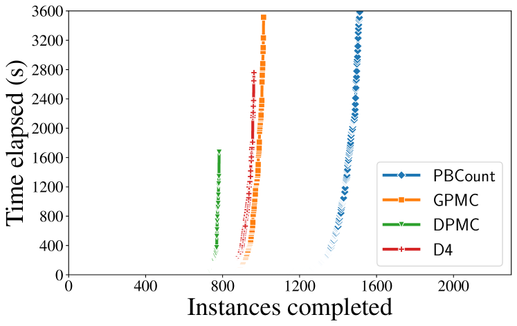
Figure 5: Cactus plot of number of benchmark instances completed by different counters. A point ($x,y$) on each line plot indicates the corresponding counter completes $x$ number of benchmarks after $y$ seconds has elapsed.

We show the cactus plot of the number of instances completed by each counter out of the 3473 benchmarks in Figure 5. The exact number of instances completed by each counter for each benchmark set is shown in Table 5.1. Additionally, we provide individual cactus plots for each set of benchmarks in the Appendix.

l—r—r—r—r Benchmarks $\mathsf{DPMC}$ $\mathsf{D4}$ $\mathsf{GPMC}$ $\mathsf{PBCount}$
Sensor placement 625 566 575 638
$\mathcal{M}$-dim knapsack 81 281 279 503
Auction 76 116 159 372
Total 782 963 1013 1513

Table 1: Number of benchmark instances completed by each counter in 3600s, higher is better.

In sensor placement benchmarks, $\mathsf{PBCount}$ count completed 638 instances, narrowly ahead of $\mathsf{DPMC}$ (625 instances), and more than $\mathsf{D4}$ (566 instances) and $\mathsf{GPMC}$ (575 instances). In multi-dimension knapsack ($\mathcal{M}$-dim knapsack) and auction benchmarks, $\mathsf{PBCount}$ significantly outperforms the competing counters. $\mathsf{PBCount}$ completed 503 $\mathcal{M}$-dim knapsack instances, around 1.8$\times$ that of $\mathsf{GPMC}$ (279 instances) and $\mathsf{D4}$ (281 instances), and 6.2$\times$ that of $\mathsf{DPMC}$ (81 instances). In auction benchmarks, $\mathsf{PBCount}$ completed 372 instances, around 2.3$\times$ that of $\mathsf{GPMC}$ (159 instances), 3.2$\times$ of $\mathsf{D4}$ (116 instances), and 4.9$\times$ of $\mathsf{DPMC}$ (76 instances). Overall, $\mathsf{PBCount}$ completed 1513 instances out of 3473 total instances, around 1.5$\times$ that of $\mathsf{GPMC}$, 1.6$\times$ of $\mathsf{D4}$, and 1.9$\times$ that of $\mathsf{DPMC}$. Note that $\mathsf{PBCount}$ achieved superior performance with minimal preprocessing over $\mathsf{GPMC}$, which has advanced preprocessing capabilities. Our results demonstrate the significant performance advantages of counting natively for PB formulas and provide an affirmative answer to RQ1.

5.2 RQ2: Analysis of compilation approaches

We now focus on the analysis of different compilation approaches: top-down (Algorithm 5), bottom-up (Algorithm 4), and dynamic (Algorithm 7). The results in Table 5.2 show that for the benchmarks, bottom-up PB constraint compilation outperforms top-down approach significantly in auction and multi-dimension knapsack and to a lesser degree sensor placement. In addition, the evaluation result also highlights that our dynamic compilation heuristic and constraint term optimization closely match the bottom-up approach, with the exception of completing 3 fewer instances in auction benchmarks. However, in the 372 auction instances completed by both bottom-up and dynamic approaches, the dynamic approach with term coefficient optimization completes the counting task faster for 257 instances. We show the scatter plot comparison in Figure 6.

l—r—r—r Benchmarks Top-down Bottom-up Dynamic
Sensor placement 580 638 638
$\mathcal{M}$-dim knapsack 109 503 503
Auction 158 375 372

Table 2: Number of benchmarks completed by $\mathsf{PBCount}$ when employing different compilation strategies, higher number indicates better performance.

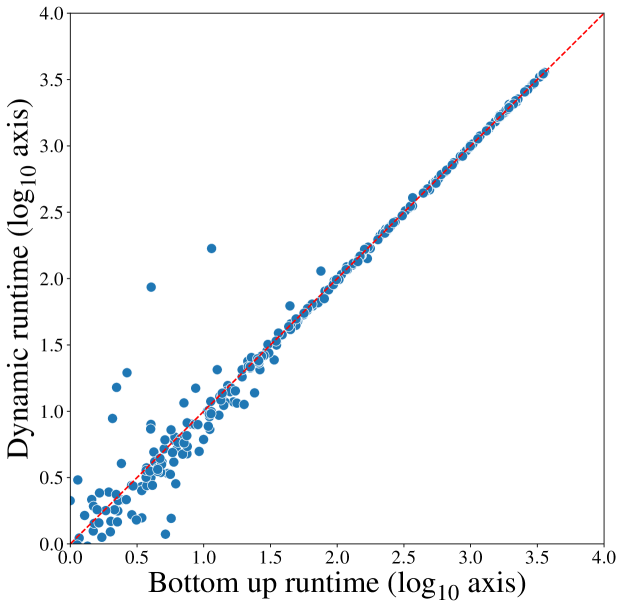
Figure 6: Dynamic vs bottom-up runtime ($\log_{10}$) for auction benchmarks. Points beneath red diagonal line indicates dynamic compilation is faster (257 points), points above otherwise (115 points).

Compilation Approach Performance Case Study

We provide an example to highlight the performance impact of the choice of compilation approach. The example involves the following PB formula in Equation 1 with a single constraint that has unique term coefficients:

$$\sum_{i=0}^{12}2^{i}x_{i+1}+\sum_{i=1}^{10}3^{i}x_{i+13}+\sum_{i=1}^{7}7^{i}x_{i+23}\geq k$$ (1)

We vary the value of $k$ in the above PB constraint from $10^{1}$ to $10^{5}$ and compare the runtime between top-down and bottom-up compilation approaches in Table 5.2. Note that bottom-up compilation takes around the same time irrespective of $k$ as there is no early termination. On the other hand for top-down compilation, the PB constraint is easily satisfied when $k$ is small and thus allows for early termination, leading to significant time savings compared to when $k$ is large. Notice that when top-down compilation is unable to terminate early, it is much slower than bottom-up compilation even when all term coefficients are unique.

l—r—r—r—r—r Approach $k$ value
$10^{1}$ $10^{2}$ $10^{3}$ $10^{4}$ $10^{5}$
Top-down 0.005 0.009 0.228 8.586 46.071
Bottom-up 6.927 7.202 7.198 7.434 6.732

Table 3: Runtime (seconds) to complete model counting for formula in Equation 1. Lower is better

l—r—r—r—r—r Approach $k$ value
$10^{1}$ $10^{2}$ $10^{3}$ $10^{4}$ $10^{5}$
Top-down 3.325 61.753 60.530 60.881 64.097
Bottom-up 0.005 0.004 0.004 0.004 0.004

Table 4: Runtime (seconds) to complete model counting for formula in Equation 1 with all coefficients set to 1.

As mentioned previously, bottom-up compilation benefits from having large numbers of same term coefficients or collisions in subset sums of coefficients. To this end, we changed all term coefficients of the PB constraint in equation 1 to $1$ and compared runtimes in Table 5.2. We observed around three orders of magnitude reduction in the runtime of the bottom-up compilation approach. In contrast, the top-down approach terminates early only in $k=10^{1}$ case and requires full enumeration in other cases. In the absence of early termination, top-down compilation approach is much slower than bottom-up compilation approach, and this is reflected in our dynamic compilation heuristic.

6 Conclusion

In this work, we introduce the first exact PB model counter, $\mathsf{PBCount}$. $\mathsf{PBCount}$ directly compiles PB formulas into ADDs, enabling us to reuse the ADD counting framework in $\mathsf{ADDMC}$. In the design of $\mathsf{PBCount}$, we introduce both top-down and bottom-up PB constraint compilation techniques and highlight the performance differences between them. While we introduced dynamic compilation heuristics to determine the per constraint compilation method and preliminary preprocessing techniques for PB formulas, it would be of interest to develop more advanced heuristics and preprocessing techniques in future works. A strong motivation is $\mathsf{PBCount}$’s performance lead over existing CNF model counters. We hope this work will gather more interest in PB formulas and PB model counting.

Acknowledgments

The authors thank Anna L.D. Latour for helping during benchmark generation. The authors thank Arijit Shaw and Jiong Yang for constructive discussions. The authors thank reviewers for providing feedback. This work was supported in part by the Grab-NUS AI Lab, a joint collaboration between GrabTaxi Holdings Pte. Ltd. and National University of Singapore, and the Industrial Postgraduate Program (Grant: S18-1198-IPP-II), funded by the Economic Development Board of Singapore. This work was supported in part by National Research Foundation Singapore under its NRF Fellowship Programme [NRF-NRFFAI1-2019-0004], Ministry of Education Singapore Tier 2 grant [MOE-T2EP20121-0011], and Ministry of Education Singapore Tier 1 Grant [R-252-000-B59-114]. The computational work for this article was performed on resources of the National Supercomputing Centre, Singapore.

Appendix

Algorithm Details

Algorithm 8 InferDecision($C$)

Input: $C$ - PB constraint with single term $a_{i}l_{i}$ where $l_{i}$ is a literal of variable $x_{i}$

Output: assignment mapping of $x_{i}$ if inferred

1:  mapping $\leftarrow[]$

2:  if $C$ is equality then

3:     if $a_{i}=k$ and $k\not=0$ then

4:        mapping $\leftarrow\mathsf{mapLitTrue(C)}$

5:     else if $k=0$ then

6:        mapping $\leftarrow\mathsf{mapLitFalse(C)}$

7:  else

8:     if ($0<k\leq a_{i}$ and $\mathsf{isPosLit}(l_{i})$) or ($a_{i}\leq k<0$ and $\mathsf{isNegLit}(l_{i})$) then

9:        mapping $\leftarrow\mathsf{mapLitTrue(C)}$

10:  return  mapping

As mentioned in the main paper, it could be possible to infer decision in variables for PB constraints that comprises of only one literal, or one term. We present the algorithm for inferring decisions as Algorithm 8, $\mathsf{InferDecision}$. Given a PB constraint $C$, there are two cases – when $C$ is an equality and when $C$ is of $\geq$ form. When $C$ is an equality, $C$ is satisfied either when its constraint constant $k=0$ (we infer literal $l_{i}$ should be false) or when $a_{i}=k$ (we infer literal $l_{i}$ should be true). When $C$ is an inequality of $\geq$ form, we can infer that literal $l_{i}$ should be true in two scenarios. The first is when $l_{i}$ is not a negated literal and that $0<k\leq a_{i}$. The second is when $l_{i}$ is a negated literal and $a_{i}\leq k<0$. In other cases, we are unable to infer a decision for variable $x_{i}$.

Algorithm 9 optimizeCompileBottomUp($T,k,eq$)

Input: $T$ - term list, $k$ - constraint value, $eq$ - input constraint equality

Output: $\psi$ - constraint ADD

1:  $T\leftarrow\mathsf{sortAscendingAbsoluteCoeff}(T)$

2:  $T^{\prime},k^{\prime}\leftarrow\mathsf{makeEveryAltCoeffPos}(T,k)$

3:  return  $\mathsf{compileConstraintBottomUp}(T^{\prime},k^{\prime},eq)$

In the main paper, Section 4, we described optimizations for the PB constraint compilation process. In particular, we mentioned that for bottom-up compilation approach, it would be desirable if the intermediate ADD is small when compiling the terms component of the given PB constraint. To that end, we show our optimizations for bottom-up constraint ADD compilation in Algorithm 9. We sort the terms in the PB constraint in ascending term coefficient magnitude, and subsequently manipulate the constraint such that adjacent term coefficients have different signs. The idea is to improve the collision rate of subset sums of coefficients so that there are fewer leaf nodes required in the intermediate ADD.

Algorithm 10 optimizeCompileTopDown($T,k,eq$)

Input: $T$ - term list, $k$ - constraint value, $eq$ - input constraint equality

Output: $\psi$ - constraint ADD

1:  $T^{\prime},k^{\prime}\leftarrow\mathsf{makeAllCoeffPos}(T,k)$

2:  $T^{\prime}\leftarrow\mathsf{sortDescendingCoeff}(T)$

3:  return  $\mathsf{compileConstraintTopDown}(T^{\prime},k^{\prime},eq)$

Similarly, we introduce optimizations for top-down constraint ADD compilation process in Algorithm 10. The main optimization idea for top-down compilation approach is to process the terms in such a manner that allows for early termination. As mentioned in the main paper, early termination can happen when PB constraint is of $\geq$ form. In particular, early termination can only take place after all terms with negative coefficients have been processed. To this end, we manipulate all term coefficients to be positive so that early termination can take place at all times. In addition, processing larger coefficients will satisfy the $\geq$ inequality sooner. As such, our optimizations included processing the terms in decending order of coefficients.

Benchmark Statistics

In this work, we generated benchmarks for various applications – sensor placement, multidimension knapsack, and combinatorial auction applications. We detail the number of variables, clauses, and constraints of the PB formula and converted CNF formula, in the rest of this section.

l—r—r—r—r Statistics # PB variable # PB constraint # CNF variable # CNF clause
Min 5 1 5 1
25% 60 4 15830 28456
50% 91 9 41900.5 77265.5
75% 131 14 80270 147022.75
Max 252 20 234777 474900

Table 5: Statistics of number variables, number of constraints and number of clauses for PB and CNF formula in the auction benchmarks

Table 6 shows the benchmark statistics for the auction setting. We show the minimum number, $25^{th}$ percentile, median, $75^{th}$ percentile, and max value for the number of variables, constraints, and clauses for both PB formula and converted CNF formula. The ‘# PB variable’ and ‘# PB constraint’ columns show statistics for the number of variables and constraints in the 1000 PB formulas (each PB formula is one benchmark), on median (‘50%’ row) the PB benchmarks have 91 variables and 9 constraints. Similarly, the numbers for the converted CNF formulas are shown under ‘# CNF variable’ and ‘# CNF clause’ columns. The CNF version of the benchmarks have on median 41900.5 variables and 77265.5 clauses, which is 4 to 5 orders of magnitude larger than that of the PB version, this strongly supports our claim that PB formulas are polynomially more succinct than CNF formulas. The observation also holds for $\mathcal{M}$-dim knapsack benchmarks (multidimension knapsack) which we show the stats for in Table 6.

l—r—r—r—r Statistics # PB variable # PB constraint # CNF variable # CNF clause
Min 5 1 28 38
25% 86.75 6 7866 14871.25
50% 164 10 25212 46340
75% 234 15 50670.5 92525.25
Max 300 20 171632 314821

Table 6: Statistics of number variables, number of constraints and number of clauses for PB and CNF formula in the $\mathcal{M}$-dim knapsack benchmarks

However, the difference is not as large in sensor placement benchmarks, because the coefficients and $k$ values are predominantly 1 and -1 except for the budget constraint which indicates the maximum number of sensors one could place. As such the sensor placement benchmarks are also more amenable to CNF encodings, unlike auction and knapsack benchmarks with different coefficients. We show the benchmark statistics for sensor placement setting in Table 6.

l—r—r—r—r Statistics # PB variable # PB constraint # CNF variable # CNF clause
Min 1 2 1 1
25% 25 291 158 539.75
50% 81.5 1210 1154 3745.5
75% 190 7056.5 3932 12902.5
Max 300 44552 7699 55514

Table 7: Statistics of number variables, number of constraints and number of clauses for PB and CNF formula in the sensor placement benchmarks

Additional Results

In the main paper, we provided a cactus plot showing the total number of benchmark instances completed by each counter. We provide the cactus plots for each set of benchmarks in Figure 7.

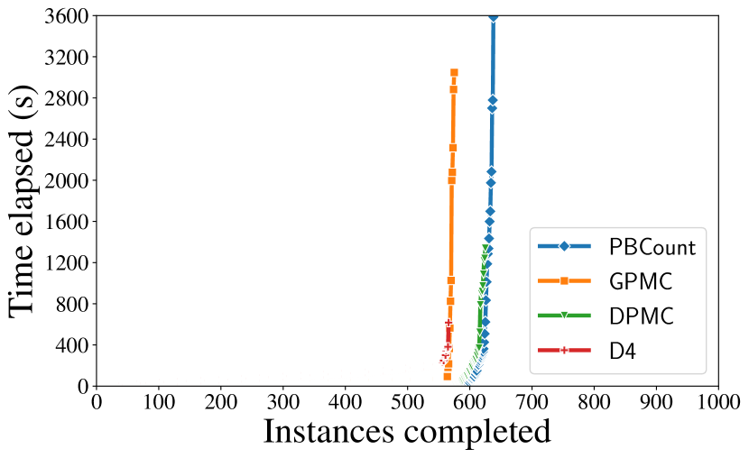
(a) Sensor placement

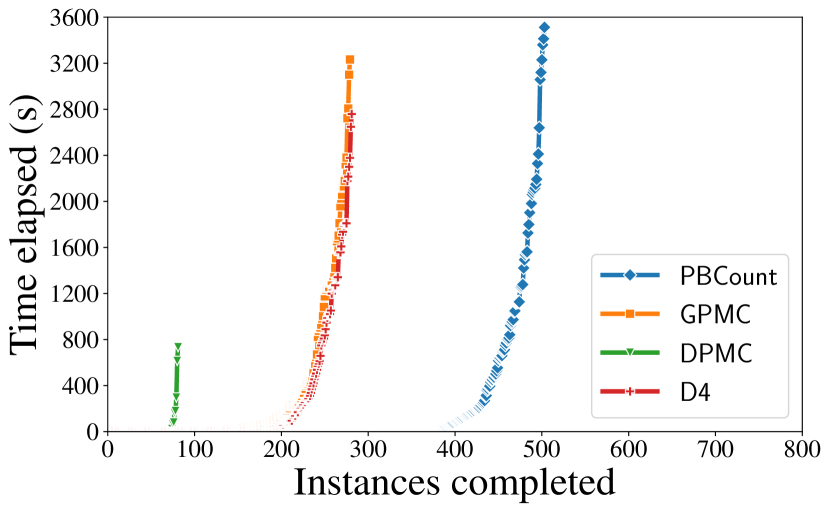
(b) $\mathcal{M}$-dim Knapsack

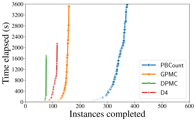
(c) Auction

Figure 7: Cactus plots of different benchmark sets. A point ($x,y$) on each line plot indicates the corresponding counter completes $x$ number of benchmarks after $y$ seconds has elapsed.

In the main paper, we showed the number of benchmarks completed by each counter. We show the number of unique benchmarks completed by each counter, along with the complete results in Table 6.

l—r—r—r—r Benchmarks $\mathsf{DPMC}$ $\mathsf{D4}$ $\mathsf{GPMC}$ $\mathsf{PBCount}$
Sensor placement 625 (2) 566 (0) 575 (0) 638 (11)
$\mathcal{M}$-dim knapsack 81 (0) 281 (13) 279 (2) 503 (242)
Auction 76 (0) 116 (0) 159 (12) 372 (229)
Total 782 (2) 963 (13) 1013 (14) 1513 (482)

Table 8: Number of benchmark instances completed by each counter in 3600s, higher is better. Number in brackets indicates number of unique instances completed by the respective solver.

In the main paper, we mentioned that $\mathsf{PBCount}$ outperforms state of the art propositional model counter $\mathsf{GPMC}$ while using minimal preprocessing techniques relative to $\mathsf{GPMC}$’s advanced preprocessing techniques. We show the number of benchmarks completed by both $\mathsf{PBCount}$ (dynamic compilation) and $\mathsf{GPMC}$ with and without preprocessing in Table 6 with 1800 seconds timeout. We were not able to completely turn off preprocessing and simplification in $\mathsf{GPMC}$, we only turned it off using the preprocessing parameter flags exposed to users by $\mathsf{GPMC}$.

l—r—r—r—r Benchmarks $\mathsf{GPMC}$ (no-pp) $\mathsf{GPMC}$ $\mathsf{PBCount}$ (no-pp) $\mathsf{PBCount}$
Sensor placement 568 570 631 633
$\mathcal{M}$-dim knapsack 255 267 484 484
Auction 120 154 347 347
Total 943 991 1462 1464

Table 9: Number of benchmarks completed by each counter with and without preprocessing (‘no-pp’ indicates no preprocessing) with 1800s timeout, higher is better.

Without preprocessing, $\mathsf{PBCount}$ completed 2 fewer benchmark instances in total while $\mathsf{GPMC}$ showed a significant performance drop by completing 48 fewer instances. We further highlight the performance impact of preprocessing to $\mathsf{PBCount}$ and $\mathsf{GPMC}$ by showing the runtime statistics in Table 6.

l—r—r—r—r Runtime statistics $\mathsf{GPMC}$ (no-pp) $\mathsf{GPMC}$ $\mathsf{PBCount}$ (no-pp) $\mathsf{PBCount}$
Min 0.00 0.00 0.00 0.00
25% 11.33 3.60 0.21 0.18
50% 47.45 18.98 0.57 0.52
75% 104.74 40.71 12.80 11.83
Max 1760.28 1800.00 1784.94 1753.13

Table 10: Runtime statistics of number benchmark instances completed by $\mathsf{PBCount}$ and $\mathsf{GPMC}$, ‘(no-pp)’ corresponds to settings where preprocessing of counter is disabled.

Additionally, we conducted experiments to further analyze the performance of top-down and bottom-up compilation approaches. In particular, we modified the auction benchmarks in two ways (a) for each PB constraint we set the term coefficient to $\pm a$ where $a$ is randomly generated, and (b) for each PB constraint we set the term coefficient to one of three randomly generated value independently ($\pm a,\pm b$ or $\pm c$). We show the results in Table 6.

l—r—r—r Benchmarks Top-down Bottom-up Dynamic
Same value (887) 236 758 757
3 values (903) 258 705 705

Table 11: Number of benchmarks completed by $\mathsf{PBCount}$ when employing different compilation strategies, with 3600s timeout, higher number indicates better performance.

The ‘same value’ row corresponds to setting (a), and we were able to get 887 non-zero count benchmarks from the original auction benchmarks. Similarly, setting (b) corresponds to the ‘3 values’ row and we were able to get 903 non-zero count benchmarks. Notice that as we increase the number of different coefficients from setting (a) to setting (b), the number of benchmarks that can be completed by bottom-up compilation decreased from 758 to 705 even when the total number of benchmarks increased from 887 to 903. We also see that the gap between top-down and bottom-up approaches is reduced with the increase in different coefficient values.

References

- Abío et al. (2011) Abío, I.; Nieuwenhuis, R.; Oliveras, A.; and Rodríguez-carbonell, E. 2011. BDDs for Pseudo-Boolean Constraints - Revisited. In International Conference on Theory and Applications of Satisfiability Testing.
- Abío et al. (2013) Abío, I.; Nieuwenhuis, R.; Oliveras, A.; and Rodríguez-carbonell, E. 2013. A Parametric Approach for Smaller and Better Encodings of Cardinality Constraints. In International Conference on Principles and Practice of Constraint Programming.
- Aziz et al. (2015) Aziz, R. A.; Chu, G.; Muise, C.; and Stuckey, P. J. 2015. #SAT: Projected Model Counting. In International Conference on Theory and Applications of Satisfiability Testing.
- Bacchus, Dalmao, and Pitassi (2003) Bacchus, F.; Dalmao, S.; and Pitassi, T. 2003. Algorithms and complexity results for #SAT and Bayesian inference. 44th Annual IEEE Symposium on Foundations of Computer Science, 2003. Proceedings.
- Bahar et al. (1993) Bahar, R. I.; Frohm, E. A.; Gaona, C. M.; Hachtel, G. D.; Macii, E.; Pardo, A.; and Somenzi, F. 1993. Algebraic decision diagrams and their applications. In International Conference on Computer Aided Design (ICCAD).
- Berre (2001) Berre, D. L. 2001. Exploiting the real power of unit propagation lookahead. Electron. Notes Discret. Math., 9: 59–80.
- Berre et al. (2018) Berre, D. L.; Marquis, P.; Mengel, S.; and Wallon, R. 2018. Pseudo-Boolean Constraints from a Knowledge Representation Perspective. In International Joint Conference on Artificial Intelligence.
- Biere, Järvisalo, and Kiesl (2021) Biere, A.; Järvisalo, M.; and Kiesl, B. 2021. Preprocessing in SAT Solving. In Handbook of Satisfiability.
- Blumrosen and Nisan (2007) Blumrosen, L.; and Nisan, N. 2007. Combinatorial Auctions, chapter 11, 267–300. Cambridge University Press, algorithmic game theory edition.
- Bryant (1986) Bryant, R. E. 1986. Graph-Based Algorithms for Boolean Function Manipulation. IEEE Transactions on Computers, C-35(8): 677–691.
- Devriendt (2020) Devriendt, J. 2020. Watched Propagation of 0-1 Integer Linear Constraints. In International Conference on Principles and Practice of Constraint Programming (CP).
- Devriendt et al. (2021) Devriendt, J.; Gocht, S.; Demirovic, E.; Nordström, J.; and Stuckey, P. J. 2021. Cutting to the Core of Pseudo-Boolean Optimization: Combining Core-Guided Search with Cutting Planes Reasoning. In AAAI Conference on Artificial Intelligence.
- Dowling and Gallier (1984) Dowling, W. F.; and Gallier, J. H. 1984. Linear-Time Algorithms for Testing the Satisfiability of Propositional Horn Formulae. J. Log. Program., 1: 267–284.
- Dudek, Phan, and Vardi (2020a) Dudek, J. M.; Phan, V. H. N.; and Vardi, M. Y. 2020a. ADDMC: Weighted Model Counting with Algebraic Decision Diagrams. In AAAI Conference on Artificial Intelligence.
- Dudek, Phan, and Vardi (2020b) Dudek, J. M.; Phan, V. H. N.; and Vardi, M. Y. 2020b. DPMC: Weighted Model Counting by Dynamic Programming on Project-Join Trees. In International Conference on Principles and Practice of Constraint Programming.
- Eén and Biere (2005) Eén, N.; and Biere, A. 2005. Effective Preprocessing in SAT Through Variable and Clause Elimination. In International Conference on Theory and Applications of Satisfiability Testing.
- Eén and Sörensson (2006) Eén, N.; and Sörensson, N. 2006. Translating Pseudo-Boolean Constraints into SAT. J. Satisf. Boolean Model. Comput., 2: 1–26.
- Elffers and Nordström (2018) Elffers, J.; and Nordström, J. 2018. Divide and Conquer: Towards Faster Pseudo-Boolean Solving. In International Joint Conference on Artificial Intelligence (IJCAI).
- Fan, Miller, and Mitra (2020) Fan, C.; Miller, K.; and Mitra, S. 2020. Fast and Guaranteed Safe Controller Synthesis for Nonlinear Vehicle Models. Computer Aided Verification, 12224: 629 – 652.
- Gens and Levner (1980) Gens, G.; and Levner, E. 1980. Complexity of approximation algorithms for combinatorial problems: a survey. SIGACT News, 12: 52–65.
- Jackson (2019) Jackson, D. 2019. Alloy: a language and tool for exploring software designs. Commun. ACM, 62.
- Korhonen and Järvisalo (2021) Korhonen, T.; and Järvisalo, M. 2021. Integrating Tree Decompositions into Decision Heuristics of Propositional Model Counters. In International Conference on Principles and Practice of Constraint Programming.
- Lagniez and Marquis (2017) Lagniez, J.-M.; and Marquis, P. 2017. An Improved Decision-DNNF Compiler. In International Joint Conference on Artificial Intelligence.
- Lai, Meel, and Yap (2021) Lai, Y.; Meel, K. S.; and Yap, R. H. C. 2021. The Power of Literal Equivalence in Model Counting. In AAAI Conference on Artificial Intelligence.
- Latour, Sen, and Meel (2023) Latour, A.; Sen, A.; and Meel, K. 2023. Solving the Identifying Code Set Problem with Grouped Independent Support. In Proceedings of the 32nd International Joint Conference on Artificial Intelligence (IJCAI23).
- Narodytska et al. (2019) Narodytska, N.; Shrotri, A. A.; Meel, K. S.; Ignatiev, A.; and Marques-Silva, J. 2019. Assessing Heuristic Machine Learning Explanations with Model Counting. In International Conference on Theory and Applications of Satisfiability Testing (SAT).
- Philipp and Steinke (2015) Philipp, T.; and Steinke, P. 2015. PBLib - A Library for Encoding Pseudo-Boolean Constraints into CNF. In International Conference on Theory and Applications of Satisfiability Testing.
- Piette, Hamadi, and Sais (2008) Piette, C.; Hamadi, Y.; and Sais, L. 2008. Vivifying Propositional Clausal Formulae. In European Conference on Artificial Intelligence.
- Ryosuke Suzuki and Sakai (2017) Ryosuke Suzuki, K. H.; and Sakai, M. 2017. Improvement of Projected Model-Counting Solver with Component Decomposition Using SAT Solving in Components. In JSAI Technical Report.
- Sharma et al. (2019) Sharma, S.; Roy, S.; Soos, M.; and Meel, K. S. 2019. GANAK: A Scalable Probabilistic Exact Model Counter. In Proceedings of International Joint Conference on Artificial Intelligence (IJCAI).
- Sinz (2005) Sinz, C. 2005. Towards an Optimal CNF Encoding of Boolean Cardinality Constraints. In International Conference on Principles and Practice of Constraint Programming (CP).
- Yang and Meel (2021) Yang, J.; and Meel, K. S. 2021. Engineering an Efficient PB-XOR Solver. In International Conference on Principles and Practice of Constraint Programming (CP).