Correlation function for the
Abstract
We have conducted a model independent analysis of the pair correlation function obtained from ultra high energy collisions, with the aim of extracting the information encoded in it related to the interaction and the coupled channel . With the present large errors at small relative momenta, we find that the information obtained about the scattering matrix suffers from large uncertainties. Even then, we are able to show that the data imply the existence of the resonance, , showing as a strong cusp close to the threshold. We also mention that the measurement of the correlation function will be essential in order to constrain more the information on dynamics that can be obtained from correlation functions.
I Introduction
Femtoscopic correlation functions are emerging as a powerful tool to learn about hadron interactions. In or collisions at very high energy, pairs of particles are measured and their production probability is divided by the equivalent probability of uncorrelated events, evaluated through the mixed event method Drijard et al. (1984); Fachini (2002); L’Hote (1994); van Eijndhoven and Wetzels (2002); Toia (2006); Kaskulov et al. (2010). There is already much experimental work on this field Acharya et al. (2017, 2019a, 2019b, 2019c, 2020a, 2020b); Collaboration et al. (2020); Acharya et al. (2021a, b, 2022a); Adamczyk et al. (2015); Adam et al. (2019); Fabbietti et al. (2021) and theoretical work goes parallel Morita et al. (2015); Ohnishi et al. (2016); Sarti et al. (2023); Morita et al. (2016); Hatsuda et al. (2017); Mihaylov et al. (2018); Haidenbauer (2019); Morita et al. (2020); Kamiya et al. (2020, 2022a, 2022b); Liu et al. (2023a); Vidana et al. (2023); Albaladejo et al. (2023a); Liu et al. (2023b, c), showing that significant information about the interaction of the measured pairs is obtained from correlation functions. While most theoretical works compare models with the results of the correlation functions, it has only been recently that model independent methods have been proposed to extract the information encoded in these correlation functions Ikeno et al. (2023); Albaladejo et al. (2023b); Feijoo et al. (2023); Molina et al. (2023), such as to conclude the possible existence of bound states, and determine scattering parameters like the scattering length and effective range of the involved channels in the interactions.
In the present work we take advantage of the existing measurements of the correlation function for production Acharya et al. (2019d, 2022b) and extract from there properties about the , interaction, among them, the existence of a resonance very close to the threshold, the . Uncertainties in observables obtained from the correlation function are evaluated through the resampling method, determining the precision demanded on the experimental data in order to get more precise values of these observables.
There is already some theoretical work on this correlation function using data from collisions Achasov and Kiselev (2018) and applying the Lednicky-Lyuboshitz approximation Lednicky and Lyuboshits (1981); Lednicky (2006) where a good reproduction of the data was obtained by using different conventions for the correlation function, that did not allow the authors to be very conclusive on the information that can be obtained from these data. Here we employ instead an improved theoretical approach based on the original Koonin-Pratt formula Koonin (1977); Pratt et al. (1990), modified to include the range of the interaction Vidana et al. (2023) and take the data from collisions of the more recent paper Acharya et al. (2022b)
II Formalism
II.1 Brief summary of the chiral unitary approach
In the chiral unitary approach Oller and Oset (1997); Kaiser (1998); Markushin (2000); Nieves and Ruiz Arriola (1999), one uses the and coupled channels and the scattering matrix given by,
| (1) |
with given by Xie et al. (2015),
Given the isospin multiplets: , , , one can easily find, for the channels, (1) , and (2) ,
| (3) |
In Eq. (1), is the diagonal meson-meson loop function, with the diagonal elements, , , given by,
| (4) |
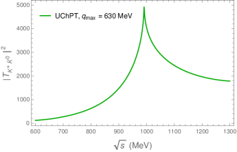
being is a regulator of the loop function which in Xie et al. (2015) is taken around MeV. The -matrix gives rise to a cusp like structure around the threshold, in agreement with the shapes obtained in recent experiments Rubin et al. (2004); Ablikim et al. (2017). The approach allows to reproduce different experiments where the is produced, as the Liang et al. (2016), the decay Molina et al. (2020), Toledo et al. (2021), among others.
II.2 Correlation functions
II.3 Inverse problem
We will make a fit to the data of the correlation function without assumming any specific interaction. The scattering matrix between the two channels, , and , is given by Eq. (1), taking a general function,
| (10) |
Since we are only interested in the region close to , we assume that the elements are constants. Then, in order to calculate and the correlation function we have a total of five parameters, three coefficients , and . These parameters are fitted to the data.
When performing a fit to the data, one obtains the parameters with large errors. This is due to the large errors of the data at small momenta but also to the strong correlations between the parameters111It is easy to see by using one channel the existence of strong correlations between the parameters and . Indeed, in that case, , and we can change and simultaneously (through ), such that does not change at the threshold.. In order to quantify uncertainties in the observables, we conduct a bootstrap procedure Press et al. (1992); Efron and Tibshirani (1994); Albaladejo et al. (2016), generating random centroids normally distributed and with the same error bars. Then we carry a fit in each case, determine the parameters and from them the values of the observables. After that, we calculate their dispersion, which gives us the uncertainties with which we can hope to obtain these magnitudes.
II.4 Observables
As we will show in the next section, we get a cusp-like structure corresponding to the resonance in the element of the scattering amplitude. Then, we also evaluate the scattering length and effective range, for the and channels, given by Ikeno et al. (2023)
| (11) |
with
| (12) |
evaluated for and . Since for the channel is open for decay, the values of the scattering parameters, , are complex for this channel, while for the channel, they must be real.
III Results
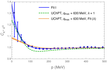
In Fig. 1 we show the correlation function obtained from Fig. 5 of Ref. Acharya et al. (2022b), taking an average of the data for TeV and TeV, and summing the systematic uncertainties (given by boxes in Fig. 5 of Acharya et al. (2022b)) to the statistical errors222The statistical errors are evaluated by taking the maximum between the average of the errors for TeV and TeV and the difference of both centroids at these two energies divided by two.. Instead of using the theoretical correlation function given by Eq. (5), an experimental parameter Acharya et al. (2022b), called correlation strength, assumming the role of an experimental efficiency, is introduced. The function to be fitted to the data is333We are thankful to Valentina Mantovani and Albert Feijoo for instructing us on these details.
| (13) |
where is the theoretical correlation function of Eq. (5), with a normalization factor around , and a flat factor also around . We take . For , when , is also which is the case of the correlation data beyond MeV/c.
We perform the following fits (where we have at least six free parameters, three elements, , , ) :
-
-
Fit I. and is a free parameter.
-
-
Fit II. is restricted in the interval , as it should be for an experimental efficiency, and is a free parameter.
-
-
Fit III. is restricted in the interval and we take .
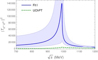
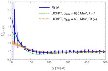
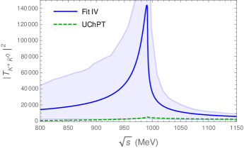
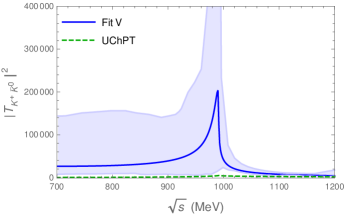
In Fig. 1 we show the result of Fit I in comparison with the one of UChPT, taking MeV and fixing the , or leaving as a fitting parameter. The value obtained is . We show the element in Fig. 2. The best fit is shown as a blue continuous line, while the error band is obtained from the resampling. We obtain a cusp like structure around the threshold. However the strength of the peak is more than two orders of magnitude larger than that of the UChPT (which is around ), and once the error band is calculated, it falls much below the result from Fit I.
In Tables 1 and 2 we show the values of the parameters of the interaction of the best fit, and also the result for the scattering parameters, for the and channels, with the uncertainties evaluated from the resampling method. Each new fit of the bootstrap procedure returns a set of parameters that take automatically into account the existing correlations. After every fit we determine the values of the observables, and from many such fits we evaluate the dispersion of these observables. As we can see, the errors of the free parameters obtained are very large, see Table 1, indicating that there are strong correlations between the parameters. As we have mentioned, this is not a problem since we are interested in the values of the observables, not in those of the parameters.
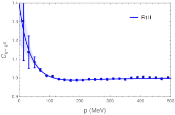
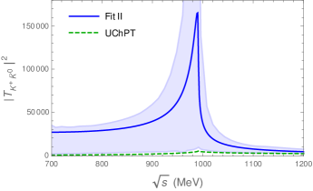
We show the results of Fit II also in Tables 1 and 2. In this case the parameter is restricted to the interval and the normalization factor in Eq. (12) is also a free parameter. The result for the correlation function is shown in Fig. 3. The normalization obtained is very close to one, , but the error band has become somewhat bigger. The result for the scattering amplitude is shown is in Fig. 4. Similarly to Fit I, a cusp related to the is clearly visible from the fit. Still the scattering amplitude for UChPT, also shown in Fig. 5 for clarity, is below the result of Fit II, but much closer to the error band than in the case of Fit I.
Next, we fix the value of , and restrict the parameter , performing Fit III. The results are shown also in Tables 1 and 2. These are very similar to the ones of Fit II, but the error bands for the correlation function and scattering amplitude obtained (omitted here since these don’t introduce new information) are slightly narrower.
In the following, we make some consideration about the errors of the experimental data. Given that the experimental data of the first three points from Fig. 5 of Ref. Acharya et al. (2022b) contain systematic errors which are indeed quite large, it is surprising that there are not such errors for energies above MeV. It is also shocking that the result of UChPT is completely different in strength, apart from the fact, that both show a cusp close to the mass of the . Thus, we propagate the systematic error of the third point around MeV to the rest of data for higher energies, and perform similar fits, labeled as IV, V, VI, in the same way as I, II, III but with the new errors. The results for the free parameters and scattering parameters are shown in Tables 1 and 2. The correlation function and scattering amplitude are depicted in Figs. 6 and 7, in comparison with the UChPT result, where we also show in Fig. 6 the result from fitting the parameter for the UChPT case. We obtain .
| Fit | ||||||
|---|---|---|---|---|---|---|
| I | ||||||
| II | ||||||
| III | ||||||
| IV | ||||||
| V | ||||||
| VI |
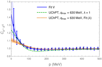
The error bands obtained in this case are very large, overlapping with the result of fitting the parameter with UChPT for the correlation function, Fig. 6, and also for the scattering amplitude and around the peak, as shown in Fig. 7. However, as shown in Table 1, in this case we observe that some samples in the resampling lead to value of out of the range , that shouldn’t be the case in principle444Note that this only happens when the experimental errors are larger and is a free parameter as in Fit IV.. Thus, we conduct Fits V and VI, restricting this parameter to . In Fit V, we leave as a free parameter. We obtain, . The results for the correlation function and scattering matrix, shown in Figs. 8 and 9, are similar to the previous cases, except for the fact that the error band of the scattering amplitude has become larger for lower energies, and the strength of the peak is slightly higher.
| Fit | ||||
|---|---|---|---|---|
| I | ||||
| II | ||||
| III | ||||
| IV | ||||
| V | ||||
| VI |
IV Conclusions
We have used the present data on the correlation function for the production in high energy scattering and have conducted fits to the data with the purpose of extracting the information on the interaction of these pairs encoded in the correlation function. We have used a model independent analysis which provides the scattering amplitudes of these pairs, from where we have seen the structure of these amplitudes and deduced the scattering length and effective range, also for the coupled channel . What we observe is that the present accuracy of the data renders an information with very large uncertainties. Within these uncertainties, it is still possible to see that the strength of peaks around the threshold, indicating that these data corroborates the existence of the resonance, which shows in recent experiments as a strong cusp around the threshold. It is clear that more precision is needed for the data at small relative momenta of the pair. Yet, this might not be sufficient to get good information. We believe that these data should be complemented with data on the correlation function of . We base this conclusion in the experience obtained from the analysis of correlation functions for the Ikeno et al. (2023) and the Molina et al. (2023). Indeed, in the former case, the analysis of the correlation functions of and (which are quite similar) allowed one to determine the existence of the state bound by about MeV, with an accuracy of only MeV (assuming errors in the data typical of present measurements of the correlation functions). On the other hand, for the latter case, using the correlation functions of the , , and , one could determine the position of the state, bound by about MeV with respect to the and MeV with respect to the threshold, with an accuracy of MeV. It is clear that the combined information of the correlation functions of coupled channels to which the state couples, is far richer than the information from one channel alone. The large uncertainties of the results obtained here are in line with the results of Achasov and Kiselev (2018), where the correlation function from collisions was reproduced with multiple, quite different scenarios, to the point that the conclusion of the authors was, “as far as we understand, it is not easy to achieve progress in this field”. Instead of using different models, we have performed a model independent analysis, with a statistical resampling method, that allows to tell us which information we can obtain and with which uncertainties. While these are definitely very large, it is still rewarding to see that the data provide information about the existence of the associated resonance. We are also more positive, in the sense that we show in which direction more information could be obtained, which is, more precision at small relative momenta, and the measurement of the correlation function. One result of the study is that the present data seem to be incompatible, or barely compatible, with the results of chiral unitary theory for the resonance, which has been very successful to explain different reactions where the resonance is explicitly seen. While the results of chiral unitary theory are qualitatively in agreement with the data for the correlation function, the apparent disagreement stems from small discrepancies in the region of MeV/c, given the extremely small experimental errors of the data. The success of the chiral unitary approach concerning the should be a reason to revise the data, or most probably the algorithm that should be used to compare with the data. Actually, the procedure to construct the correlation function dividing the probability to find a pair from a single event, by the probability of the mixed events, might require some revision, since the mixed event probability is not fully absent from correlations.
The results and discussion carried here should serve as a motivation to perform new measurements and also look for an adequate theoretical algorithm to compare with experiment. This would also allow one to obtain low energy data for the and interaction, as scattering lengths and effective ranges, which would be most welcome.
V Acknowledgments
R. M. acknowledges support from the CIDEGENT program with Ref. CIDEGENT/2019/015, the Spanish Ministerio de Economia y Competitividad and European Union (NextGenerationEU/PRTR) by the grant with Ref. CNS2022-13614. L. S. G. acknowledges supports from the National Natural Science Foundation of China under Grants No.11975041 and No.11961141004. This work is also partly supported by the Spanish Ministerio de Economia y Competitividad (MINECO) and European FEDER funds under Contracts No. FIS2017-84038-C2-1-P B, PID2020-112777GB-I00, and by Generalitat Valenciana under contract PROMETEO/2020/023. This project has received funding from the European Union Horizon 2020 research and innovation programme under the program H2020-INFRAIA-2018-1, grant agreement No. 824093 of the STRONG-2020 project.
References
- Drijard et al. (1984) D. Drijard, H. G. Fischer, and T. Nakada, Nucl. Instrum. Meth. A 225, 367 (1984).
- Fachini (2002) P. Fachini (STAR), J. Phys. G 28, 1599 (2002), eprint nucl-ex/0203019.
- L’Hote (1994) D. L’Hote, Nucl. Instrum. Meth. A 337, 544 (1994).
- van Eijndhoven and Wetzels (2002) N. van Eijndhoven and W. Wetzels, Nucl. Instrum. Meth. A 482, 513 (2002), eprint hep-ph/0101084.
- Toia (2006) A. Toia (PHENIX), Nucl. Phys. A 774, 743 (2006), eprint nucl-ex/0510006.
- Kaskulov et al. (2010) M. Kaskulov, E. Hernandez, and E. Oset, Eur. Phys. J. A 46, 223 (2010), eprint 1003.2363.
- Acharya et al. (2017) S. Acharya et al. (ALICE), Phys. Lett. B 774, 64 (2017), eprint 1705.04929.
- Acharya et al. (2019a) S. Acharya et al. (ALICE), Phys. Rev. C 99, 024001 (2019a), eprint 1805.12455.
- Acharya et al. (2019b) S. Acharya et al. (ALICE), Phys. Rev. Lett. 123, 112002 (2019b), eprint 1904.12198.
- Acharya et al. (2019c) S. Acharya et al. (ALICE), Phys. Lett. B 797, 134822 (2019c), eprint 1905.07209.
- Acharya et al. (2020a) S. Acharya et al. (ALICE), Phys. Lett. B 805, 135419 (2020a), eprint 1910.14407.
- Acharya et al. (2020b) S. Acharya et al. (ALICE), Phys. Rev. Lett. 124, 092301 (2020b), eprint 1905.13470.
- Collaboration et al. (2020) A. Collaboration et al. (ALICE), Nature 588, 232 (2020), [Erratum: Nature 590, E13 (2021)], eprint 2005.11495.
- Acharya et al. (2021a) S. Acharya et al. (ALICE), Phys. Lett. B 822, 136708 (2021a), eprint 2105.05683.
- Acharya et al. (2021b) S. Acharya et al. (ALICE), Phys. Rev. Lett. 127, 172301 (2021b), eprint 2105.05578.
- Acharya et al. (2022a) S. Acharya et al. (ALICE), Phys. Rev. D 106, 052010 (2022a), eprint 2201.05352.
- Adamczyk et al. (2015) L. Adamczyk et al. (STAR), Phys. Rev. Lett. 114, 022301 (2015), eprint 1408.4360.
- Adam et al. (2019) J. Adam et al. (STAR), Phys. Lett. B 790, 490 (2019), eprint 1808.02511.
- Fabbietti et al. (2021) L. Fabbietti, V. Mantovani Sarti, and O. Vazquez Doce, Ann. Rev. Nucl. Part. Sci. 71, 377 (2021), eprint 2012.09806.
- Morita et al. (2015) K. Morita, T. Furumoto, and A. Ohnishi, Phys. Rev. C 91, 024916 (2015), eprint 1408.6682.
- Ohnishi et al. (2016) A. Ohnishi, K. Morita, K. Miyahara, and T. Hyodo, Nucl. Phys. A 954, 294 (2016), eprint 1603.05761.
- Sarti et al. (2023) V. M. Sarti, A. Feijoo, I. Vidaña, A. Ramos, F. Giacosa, T. Hyodo, and Y. Kamiya (2023), eprint 2309.08756.
- Morita et al. (2016) K. Morita, A. Ohnishi, F. Etminan, and T. Hatsuda, Phys. Rev. C 94, 031901 (2016), [Erratum: Phys.Rev.C 100, 069902 (2019)], eprint 1605.06765.
- Hatsuda et al. (2017) T. Hatsuda, K. Morita, A. Ohnishi, and K. Sasaki, Nucl. Phys. A 967, 856 (2017), eprint 1704.05225.
- Mihaylov et al. (2018) D. L. Mihaylov, V. Mantovani Sarti, O. W. Arnold, L. Fabbietti, B. Hohlweger, and A. M. Mathis, Eur. Phys. J. C 78, 394 (2018), eprint 1802.08481.
- Haidenbauer (2019) J. Haidenbauer, Nucl. Phys. A 981, 1 (2019), eprint 1808.05049.
- Morita et al. (2020) K. Morita, S. Gongyo, T. Hatsuda, T. Hyodo, Y. Kamiya, and A. Ohnishi, Phys. Rev. C 101, 015201 (2020), eprint 1908.05414.
- Kamiya et al. (2020) Y. Kamiya, T. Hyodo, K. Morita, A. Ohnishi, and W. Weise, Phys. Rev. Lett. 124, 132501 (2020), eprint 1911.01041.
- Kamiya et al. (2022a) Y. Kamiya, K. Sasaki, T. Fukui, T. Hyodo, K. Morita, K. Ogata, A. Ohnishi, and T. Hatsuda, Phys. Rev. C 105, 014915 (2022a), eprint 2108.09644.
- Kamiya et al. (2022b) Y. Kamiya, T. Hyodo, and A. Ohnishi, Eur. Phys. J. A 58, 131 (2022b), eprint 2203.13814.
- Liu et al. (2023a) Z.-W. Liu, J.-X. Lu, and L.-S. Geng, Phys. Rev. D 107, 074019 (2023a), eprint 2302.01046.
- Vidana et al. (2023) I. Vidana, A. Feijoo, M. Albaladejo, J. Nieves, and E. Oset, Phys. Lett. B 846, 138201 (2023), eprint 2303.06079.
- Albaladejo et al. (2023a) M. Albaladejo, J. Nieves, and E. Ruiz-Arriola, Phys. Rev. D 108, 014020 (2023a), eprint 2304.03107.
- Liu et al. (2023b) Z.-W. Liu, J.-X. Lu, M.-Z. Liu, and L.-S. Geng, Phys. Rev. D 108, L031503 (2023b), eprint 2305.19048.
- Liu et al. (2023c) Z.-W. Liu, K.-W. Li, and L.-S. Geng, Chin. Phys. C 47, 024108 (2023c), eprint 2201.04997.
- Ikeno et al. (2023) N. Ikeno, G. Toledo, and E. Oset, Phys. Lett. B 847, 138281 (2023), eprint 2305.16431.
- Albaladejo et al. (2023b) M. Albaladejo, A. Feijoo, I. Vidaña, J. Nieves, and E. Oset (2023b), eprint 2307.09873.
- Feijoo et al. (2023) A. Feijoo, L. R. Dai, L. M. Abreu, and E. Oset (2023), eprint 2309.00444.
- Molina et al. (2023) R. Molina, C.-W. Xiao, W.-H. Liang, and E. Oset (2023), eprint 2310.12593.
- Acharya et al. (2019d) S. Acharya et al. (ALICE), Phys. Lett. B 790, 22 (2019d), eprint 1809.07899.
- Acharya et al. (2022b) S. Acharya et al. (ALICE), Phys. Lett. B 833, 137335 (2022b), eprint 2111.06611.
- Achasov and Kiselev (2018) N. N. Achasov and A. V. Kiselev, Phys. Rev. D 97, 036015 (2018), eprint 1711.08777.
- Lednicky and Lyuboshits (1981) R. Lednicky and V. L. Lyuboshits, Yad. Fiz. 35, 1316 (1981).
- Lednicky (2006) R. Lednicky, Nucl. Phys. A 774, 189 (2006), eprint nucl-th/0510020.
- Koonin (1977) S. E. Koonin, Phys. Lett. B 70, 43 (1977).
- Pratt et al. (1990) S. Pratt, T. Csorgo, and J. Zimanyi, Phys. Rev. C 42, 2646 (1990).
- Oller and Oset (1997) J. A. Oller and E. Oset, Nucl. Phys. A 620, 438 (1997), [Erratum: Nucl.Phys.A 652, 407–409 (1999)], eprint hep-ph/9702314.
- Kaiser (1998) N. Kaiser, Eur. Phys. J. A 3, 307 (1998).
- Markushin (2000) V. E. Markushin, Eur. Phys. J. A 8, 389 (2000), eprint hep-ph/0005164.
- Nieves and Ruiz Arriola (1999) J. Nieves and E. Ruiz Arriola, Phys. Lett. B 455, 30 (1999), eprint nucl-th/9807035.
- Xie et al. (2015) J.-J. Xie, L.-R. Dai, and E. Oset, Phys. Lett. B 742, 363 (2015), eprint 1409.0401.
- Rubin et al. (2004) P. Rubin et al. (CLEO), Phys. Rev. Lett. 93, 111801 (2004), eprint hep-ex/0405011.
- Ablikim et al. (2017) M. Ablikim et al. (BESIII), Phys. Rev. D 95, 032002 (2017), eprint 1610.02479.
- Liang et al. (2016) W.-H. Liang, J.-J. Xie, and E. Oset, Eur. Phys. J. C 76, 700 (2016), eprint 1609.03864.
- Molina et al. (2020) R. Molina, J.-J. Xie, W.-H. Liang, L.-S. Geng, and E. Oset, Phys. Lett. B 803, 135279 (2020), eprint 1908.11557.
- Toledo et al. (2021) G. Toledo, N. Ikeno, and E. Oset, Eur. Phys. J. C 81, 268 (2021), eprint 2008.11312.
- Press et al. (1992) W. Press, S. Teukolsky, W. Vetterling, and B. Flannery, Numerical Recipes in FORTRAN: The Art of Scientific Computing (Cambridge University Press, 1992), 2nd ed.
- Efron and Tibshirani (1994) B. Efron and R. J. Tibshirani, An Introduction to the Bootstrap (Chapman & Hall, New York, NY, 1994).
- Albaladejo et al. (2016) M. Albaladejo, D. Jido, J. Nieves, and E. Oset, Eur. Phys. J. C 76, 300 (2016), eprint 1604.01193.