Outcomes truncated by death in RCTs: a simulation study on the survivor average causal effect

Stefanie von Felten^1,∗, Chiara Vanetta^1,2, Christoph M. Rüegger³, Sven Wellmann⁴ & Leonhard Held¹

¹Department of Biostatistics at Epidemiology, Biostatistics and Prevention Institute, University of Zurich, Hirschengraben 84, CH-8001 Zurich, Switzerland
²Biostatistics and Research Decision Sciences, MSD, The Circle 66, CH-8058 Zurich, Switzerland
³Newborn Research, Department of Neonatology, University Hospital Zurich, University of Zurich, Frauenklinikstrasse 10, CH-8091 Zürich, Switzerland
⁴Department of Neonatology, University Children’s Hospital Regensburg, Hospital St Hedwig of the Order of St John, University of Regensburg, Steinmetzstraße 1-3, D-93049 Regensburg, Germany
^∗Corresponding author: e-mail: stefanie.vonfelten@uzh.ch, Phone: +41-44-634-46-44

Abstract

Continuous outcome measurements truncated by death present a challenge for the estimation of unbiased treatment effects in randomized controlled trials (RCTs). One way to deal with such situations is to estimate the survivor average causal effect (SACE), but this requires making non-testable assumptions. Motivated by an ongoing RCT in very preterm infants with intraventricular hemorrhage, we performed a simulation study to compare a SACE estimator with complete case analysis (CCA, benchmark for a biased analysis) and an analysis after multiple imputation of missing outcomes. We set up 9 scenarios combining positive, negative and no treatment effect on the outcome (cognitive development) and on survival at 2 years of age. Treatment effect estimates from all methods were compared in terms of bias, mean squared error and coverage with regard to two estimands: the treatment effect on the outcome used in the simulation and the SACE, which was derived by simulation of both potential outcomes per patient. Despite targeting different estimands (principal stratum estimand, hypothetical estimand), the SACE-estimator and multiple imputation gave similar estimates of the treatment effect and efficiently reduced the bias compared to CCA. Also, both methods were relatively robust to omission of one covariate in the analysis, and thus violation of relevant assumptions. Although the SACE is not without controversy, we find it useful if mortality is inherent to the study population. Some degree of violation of the required assumptions is almost certain, but may be acceptable in practice.

Keywords:

Estimand; Multiple Imputation; Principal Stratification; SACE

1 Introduction

Analysis by the intention-to-treat (ITT) principle was recommended for the primary analysis of randomized clinical trials (RCTs) by the ICH E9, (1998) guideline and is still regarded the gold standard for most RCTs. Analysis by ITT, including all randomized patients and analyzing them by the randomized treatment, irrespective of whether this treatment was received exactly as planned, best preserves the benefits of randomization and estimates the effect of a “treatment policy”. However, the latter may not always represent the most relevant “estimand”, and this is addressed in the ICH E9 , 2020 (R1) addendum. While the addendum undisputably includes the treatment policy strategy (conform with ITT), it discusses several alternative strategies to choose an estimand in the light of “intercurrent events”. Intercurrent events occur between randomization and outcome measurement, and thus affect the interpretation or existence of the latter. Examples include switching to a different treatment, treatment discontinuation, or death. Some strategies mentioned in the addendum (namely hypothetical and principal stratum strategies) require “causal inference” techniques involving potential outcomes (Imbens and Rubin,, 2015; Hernán and Robins,, 2020). While these techniques were originally designed to draw causal inference from observational data, they have a role in RCTs when we can no longer compare like with like due to the presence of intercurrent events.

The most drastic intercurrent event in a trial is a patient’s death. The event of death is a terminal event, for which the ICH E9 , 2020 (R1) addendum states that “in general, the treatment policy strategy cannot be implemented for intercurrent events that are terminal events, since values for the variable after the intercurrent event do not exist. For example, an estimand based on this strategy cannot be constructed with respect to a variable that cannot be measured due to death”. In an RCT with a time-to-event outcome death may be treated as a competing risk or it may be included in the primary outcome using a “composite variable strategy”. However, estimation of a causal treatment effect with death as intercurrent event is more challenging in an RCT with a continuous outcome, in particular if this variable is assessed only once.

An example of such an RCT is the EpoRepair trial, an ongoing placebo controlled, parallel group, double-blind RCT on the effect of erythropoietin (Epo) for the repair of cerebral injury in very preterm infants suffering from intraventricular hemorrhage (Rüegger et al.,, 2015; Wellmann et al.,, 2022). The primary outcome is the composite intelligence quotient (IQ) at five years of age measured using the Kaufmann Assessment Battery for Children (K-ABC). Cognitive development at two years of age, measured using the subscore for cognition of the Bayley Scales of Infant and Toddler Development (BSID-III), is a secondary outcome. Both, IQ and cognitive development are measured only once. The EpoRepair trial randomized 121 preterm infants to Epo or Placebo in a 1:1 fashion. However, 19 (15.7 %) of these vulnerable infants died before the age of two years (15 died before term equivalent age). How should the effect of the intervention (Epo) on IQ or on cognitive development be estimated in this case, or more conceptually, which estimand should be targeted, when a considerable proportion of outcome measurements is truncated by death?

One commonly used ad hoc solution to the problem is to restrict the analysis to the survivors (if all survivors have a measurement of the outcome) or more generally, to complete cases. In fact, a systematic review of RCTs published in the top medical journals (Bell et al.,, 2014) revealed that 95 % of the trials reported missing outcome data (median 9 %, range 0–70 %), and that complete case analysis was the most commonly used method to handle missing data in the primary analysis (45 % of trials included). However, it is well-known that complete case analysis leads to biased estimates of the treatment effect, as it corresponds to a nonrandomized comparison (see for example CHMP,, 2010). No bias would occur only when outcome measurements are "missing completely at random", i.e., the missingness is neither related to the assigned treatment nor to any characteristics of the patients. The size of the bias depends on the amount of missing or truncated observations and on their relation with the assigned treatment. A relationship with the patients response to the treatment is often likely, and differing proportions of missing observations between trial arms may add to this concern (Vickers and Altman,, 2013). Complete case analysis does also not conform with any of the strategies outlined in the ICH E9(R1) addendum.

Another ad hoc solution may be to treat the truncated outcomes as missing outcome measurements and use multiple imputation to recover the missing information. The underlying assumption of multiple imputation is that measurements are “missing at random”, which means that the missingness can be explained by observed data. Multiple imputation has been recommended for analyzing trials with missing data (but recommendations are not restricted to trials) and is known to be a better choice than single imputation methods (White et al.,, 2011; Groenwold et al.,, 2012; Vickers and Altman,, 2013). A strength of multiple imputation is that the uncertainty about the imputations can be taken into account using Rubin’s rules (Rubin,, 1987) to combine the estimates from the imputed data sets. With the availability of software to generate imputations and to combine effect size estimates, for instance in the R packages mice (van Buuren and Groothuis-Oudshoorn,, 2011) or Amelia (Honaker et al.,, 2011) this method has become increasingly popular. Multiple imputation is certainly a good choice for imputing missing outcomes if they would have been observable. However, outcome measurements truncated by death are not just a missing data problem: they are not defined (the IQ of a child who died before the IQ could be measured is not defined). While using multiple imputation allows to analyze all randomized patients (including those who died) the estimated causal treatment effect is “hypothetical”, and for a scenario in which no patient would have died. Such a “hypothetical strategy” is usually more meaningful if the intercurrent event (unlike death) could be avoided by design in a future trial. Nevertheless, in practice multiple imputation may sometimes be used to analyze trials with outcomes truncated by death, especially if truncation by death accounts for only part of the missing outcomes. This is what was planned for the EpoRepair trial (Rüegger et al.,, 2015). Or, multiple imputation may be used to impute missing outcomes of survivors only, which may be of limited use if some observations are truncated by death.

An alternative causal effect of the treatment could be estimated using principal stratification (Robins,, 1986; Frangakis and Rubin,, 2002) to estimate the survivor average causal effect (SACE, introduced by Rubin,, 2006), i.e., the treatment effect in those patients who would have survived under both treatments. A related concept is the complier average causal effect (CACE, Angrist et al.,, 1996). Principal stratification is based on stratifying patients conditional on potential outcomes of a post-randomization variable, such as the event of death. The focus is then either on the "principal stratum" in which an event would occur on all treatments or would not occur on any of the treatments. In the case of the SACE, the focus is on the principal stratum of "always survivors", those patients who would not have died under any of the treatments. Principal stratum strategies are one of the five strategies mentioned in the ICH E9(R1) addendum on estimands and sensitivity analysis in RCTs (ICH E9 , 2020, R1), and have gained in popularity in recent years. The strategy may be of particular interest if an intercurrent event in a specific population cannot be avoided by design, as it is unfortunately the case with death among very preterm infants or in other vulnerable or severely ill populations. Bornkamp et al., (2021) discuss the role of principal stratum estimands in drug development, give examples of research questions that may be addressed and give an overview of assumptions required for estimation. A comprehensive tutorial on using principal stratification in the analysis of clinical trials can be found in Lipkovich et al., (2022). However, since the principal strata are not observable, determining the patients who belong to the principal stratum of interest and estimating principal stratum effects rely on strong, untestable assumptions. These limitations lead to criticism with regard to this method, and alternatives have been proposed (see for example Stensrud et al.,, 2022).

It seems that there is still limited awareness of the fact that outcomes truncated by death are not missing data in the usual sense. Further, if truncation by death is recognized as an issue, the choice of the estimand remains challenging. We therefore performed a simulation study to compare complete case analysis (known to be biased in most cases), an analysis after multiple imputation (targeting a hypothetical estimand), and an analysis using a specific estimator of the SACE proposed by Hayden et al., (2005). The three methods are compared across 9 scenarios combining positive, negative and no treatment effect on the outcome and on survival with regard to bias, mean squared error and coverage regarding two types of true effect: 1) the treatment effect on the outcome used in the simulation and 2) the SACE derived from the simulated observed and counterfactual data. The EpoRepair trial was used as motivating example, and the simulated data resemble those from this trial. With our work we wish to promote awareness of the issue of outcomes truncated by death among applied statisticans and clinicians, and methodological knowledge of how it could be dealt with.

2 Methods

We planned our simulation study by writing a simulation study protocol in advance (available on https://osf.io/zafw3), following the recommendations of Burton et al., (2006). For the shorter description of the methods here we adopted the ADEMP structure proposed for planning and reporting of simulation studies by Morris et al., (2019). We consider our simulation study as a "neutral comparison study" (Boulesteix et al.,, 2013), because we compare three existing methods (rather than a new method with existing methods), which we have not developed ourselves, using evaluation criteria (bias, mean squared error and coverage) that were chosen in a rational way and were defined in the simulation study protocol in advance.

2.1 Aims

The aim of our simulation study is to evaluate the performance of three different methods to estimate the treatment effect from a parallel group RCT when the primary outcome is truncated by death for a relevant proportion of the patients randomized. We thereby wish to illustrate the challenge of estimating causal effects with outcomes truncated by death with a focus on applied statisticians and clinicians in clinical research as target readers.

2.2 Data-generating mechanisms

We simulated data from an RCT similar to the ongoing, placebo controlled, double-blind EpoRepair trial on the effect of erythropoietin for the repair of cerebral injury in very preterm infants suffering from intraventricular hemorrhage (Rüegger et al.,, 2015; Wellmann et al.,, 2022). Available data from EpoRepair were used as a basis, but we modified certain aspects to create the different scenarios for our simulation study. The outcome for this simulation study is cognitive development at two years of age (a secondary outcome in EpoRepair), measured using the subscore for cognition of the Bayley Scales of Infant and Toddler Development (BSID-III), hereafter referred to as outcome. We included gestational age (days), head circumference at birth (cm), socioeconomic status (SES, ordinal, score from 2 to 12, Largo et al.,, 1989) and Apgar score five min after birth (ordinal, from 1 to 10) as covariates $X_{1}$ to $X_{4}$.

We simulated data sets with a sample size of $n$=500 patients. This is a realistic sample size for an RCT and appropriate for the methods comparison in this simulation study, but larger than the size of the EpoRepair trial for which only 121 patients were included (Wellmann et al.,, 2022). We simulated the Apgar score based on the distribution observed in EpoRepair. We then simulated gestational age and head circumference as multivariate normal variables in each Apgar score category, using the means of these variables observed in each Apgar category with a constant variance-covariance matrix (estimated from EpoRepair) over all categories to avoid the simulation being too data-driven. SES was simulated based on its observed distribution within Apgar score categories. The patients $i=1,\ldots,n$ were then randomly assigned to one of two treatments $z=0,1$; 250 patients received the Placebo control ($z=0$) and 250 received the intervention Epo ($z=1$).

The outcome $Y$ was simulated using the regression coefficients $b_{1}$, $b_{2}$ and $b_{3}$ of the covariates gestational age, head circumference and SES ($X_{1}$, $X_{2}$, and $X_{3}$) on the outcome, as estimated from the EpoRepair data, and a treatment effect $b_{z}$ on the outcome (mean difference Epo vs. Placebo), which we varied between simulation scenarios as $-5$, $0$ or $5$. Survival $S$ was simulated using the regression coefficients $\tilde{b}_{1}$, $\tilde{b}_{2}$ and $\tilde{b}_{4}$ of the covariates gestational age, head circumference and Apgar score ($X_{1}$, $X_{2}$, and $X_{4}$) on survival as estimated from the EpoRepair data, and a treatment effect $\tilde{b}_{z}$ on survival (log odds ratio Epo vs. Placebo), which we varied again between simulation scenarios as -0.693, 0, or 0.693 (corresponding to odds ratios of 0.5, 1 and 2, respectively). With this simulation procedure we aimed at an overall survival probability around 84%, similar to the EpoRepair trial.

In addition to simulating data that could be observed, i.e., data under the allocated (and received) treatment, we simulated counterfactual data. Using the same settings as described above, we simulated outcome and survival under the corresponding other treatment for each patient. So, for each patient $i$, we simulated the outcome under treatment, $Y_{i}(z=1)$, and control, $Y_{i}(z=0)$:

$$Y_{i}(1) \sim N(b_{0}+b_{1}\,X_{1,i}+b_{2}\,X_{2,i}+b_{3}\,X_{3,i}+b_{z},\sigma^{2})$$ (1)

$$Y_{i}(0) \sim N(b_{0}+b_{1}\,X_{1,i}+b_{2}\,X_{2,i}+b_{3}\,X_{3,i},\sigma^{2})$$ (2)

and then survival under treatment, $S_{i}(z=1)$, and control, $S_{i}(z=0)$:

$$S_{i}(1) \sim\text{Bernoulli}(p_{i}(1)),\quad\quad p_{i}(1)=\text{logit}^{-1}(\tilde{b}_{0}+\tilde{b}_{1}\,X_{1,i}+\tilde{b}_{2}\,X_{2,i}+\tilde{b}_{4}\,X_{4,i}+\tilde{b}_{z})$$ (3)

$$S_{i}(0) \sim\text{Bernoulli}(p_{i}(0)),\quad\quad p_{i}(0)=\text{logit}^{-1}(\tilde{b}_{0}+\tilde{b}_{1}\,X_{1,i}+\tilde{b}_{2}\,X_{2,i}+\tilde{b}_{4}\,X_{4,i})$$ (4)

Table 1 shows the nine simulation scenarios that we assessed in our simulation study, which result from a fully factorial arrangement of the treatment effects on outcome and survival. For simplicity, we assumed no drop-outs due to withdrawal of informed consent or loss to follow-up for other reasons than death.

Table 1: Overview of simulation scenarios.

Scenario	Treatment effect on Outcome		Treatment effect on Survival
	Mean difference (MD)		Odds ratio (OR)
A	5	(outcome increased)	2	(survival probability higher)
B	5	(outcome increased)	1	(no effect)
C	5	(outcome increased)	0.5	(survival probability lower)
D	0	(no effect)	2	(survival probability higher)
E	0	(no effect)	1	(no effect)
F	0	(no effect)	0.5	(survival probability lower)
G	-5	(outcome decreased)	2	(survival probability higher)
H	-5	(outcome decreased)	1	(no effect)
I	-5	(outcome decreased)	0.5	(survival probability lower)

2.3 Estimands

The estimates derived by the three methods (see Section 2.4) were compared in terms of bias, mean squared error and coverage with regard to two estimands. The first estimand $\theta_{1}$ is the treatment effect on the outcome used in the simulation, equivalent to $b_{z}$. $\theta_{1}$ is a hypothetical estimand in the presence of mortality and represents the causal effect of the treatment on the outcome in the absence of mortality. The second estimand $\theta_{2}$ is the survivor average causal effect (SACE), the treatment effect on the “always survivors”, the patients who would have survived under both treatments. $\theta_{2}$ is a principal stratum estimand and is relevant here, because mortality cannot be eliminated in the populuation at hand, and because a treatment effect on survival cannot be ruled out.

While $\theta_{1}$ is defined by the simulation scenarios, $\theta_{2}$ is a priori unknown. We thus used the simulated observed and counterfactual data to derive $\theta_{2s}$ for each simulation $s=1,\dots,n_{\text{sim}}$. Given the simulated observed outcome $Y_{i}(z)$ and the simulated counterfactual outcome $Y_{i}(1-z)$, the principal stratum of always survivors can be identified and $\theta_{2s}$ can be approximated as (as defined in Equation 1 of Hayden et al., (2005)):

$$\theta_{2s}=\frac{\frac{1}{n}\sum_{i}\{Y_{i}(1)-Y_{i}(0)\}S_{i}(1)S_{i}(0)}{\frac{1}{n}\sum_{i}S_{i}(0)S_{i}(1)}=\frac{\sum_{i}\{Y_{i}(1)-Y_{i}(0)\}S_{i}(1)S_{i}(0)}{\sum_{i}S_{i}(0)S_{i}(1)}$$ (5)

$Y_{i}(1)$ and $Y_{i}(0)$ are the outcomes of patient $i$ on treatment and control, and $S_{i}(1)$ and $S_{i}(0)$ are survival of patient $i$ under treatment and control, respectively (if $S_{i}(1)=1$, patient $i$ survived on treatment, if $S_{i}(1)=0$, patient $i$ died on treatment; if $S_{i}(0)=1$ patient $i$ survived on control, if $S_{i}(0)=0$ patient $i$ died on control). To have one estimand per scenario, we then averaged over all simulations to derive $\theta_{2}$ as $\frac{1}{n_{\text{sim}}}\sum\limits_{s=1}^{n_{\text{sim}}}\theta_{2s}$. Note that $\theta_{2}$ is strictly speaking an estimate of the SACE but serves as the estimand in our simulation study. An alternative method to derive $\theta_{2}$ that was listed in the simulation study protocol was omitted, since it was less intuitive and results were very similar.

2.4 Methods to be evaluated

We used the SACE estimator proposed by (Hayden et al.,, 2005, Equation 4), hereafter referred to as SACE estimator, and compare it with complete case analysis and with analysis after multiple imputation. Complete case analysis was performed on the survivors only and is used as a benchmark for a biased analysis in most situations, since the treatment effect on survivors is not a randomized comparison. Only in the absence of mortality or if survival is unaffected by treatment would complete case analysis provide an unbiased estimator for both, $\theta_{1}$ and $\theta_{2}$, which then coincide with the treatment effect on survivors. The treatment effect estimate derived by analysis of multiply imputed data can be expected to be close to $\theta_{1}$, independent of the treatment effect on survival. Complete case analysis and the SACE estimator do not conform with the intention-to-treat (ITT) principle, as only a subset of patients is analyzed. In contrast, multiple imputation conforms with the ITT principle but creates unobservable (hypothetical) data.

As previously mentioned, the SACE is not identifiable without strong assumptions. A comprehensive overview of principal stratification methods and their underlying assumptions is given in Lipkovich et al., (2022). Hayden et al., make the stable unit treatment value assumption (SUTVA, Rubin,, 1980) and the explainable nonrandom survival assumption (Robins,, 1998; Hayden et al.,, 2005, adapted from explainable nonrandom noncompliance). The SUTVA implies that a subject’s observed outcome is the same as (consistent with) the potential outcome associated with the treatment that the subject was assigned/randomized to and that the subject’s potential outcomes do not depend on (or interfer with) the treatment assigned to other subjects (Bornkamp et al.,, 2021; Lipkovich et al.,, 2022). The SUTVA needs to be made by most principal stratification methods (and other causal inference approaches), since it allows to connect potential and observed outcomes at an individual patient level. One reason for choosing Hayden’s SACE estimator was that it neither relies on the monotonicity assumption nor on the exclusion restriction assumption (two other common assumptions), which are both unrealistic in the context of the SACE and the EpoRepair study. Monotonicity would imply that patients who die on the experimental treatment would also die on the control treatment, i.e., that there are no control-only survivors. Exclusion restriction may be reasonable when the aim is to estimate the CACE, where it would imply that potential outcomes for never-takers and always-takers are the same, but not for the SACE, where it would imply that potential outcomes of always-survivors and never-survivors (sometimes called the doomed) would be the same. Instead, Hayden’s SACE estimator relies on modeling to identify strata membership based on observed baseline covariates, assuming explainable nonrandom survival:

$$S_{i}(z) \mathchoice{\mathrel{\hbox to0.0pt{$\displaystyle\perp$\hss}\mkern 2.0mu{\displaystyle\perp}}}{\mathrel{\hbox to0.0pt{$\textstyle\perp$\hss}\mkern 2.0mu{\textstyle\perp}}}{\mathrel{\hbox to0.0pt{$\scriptstyle\perp$\hss}\mkern 2.0mu{\scriptstyle\perp}}}{\mathrel{\hbox to0.0pt{$\scriptscriptstyle\perp$\hss}\mkern 2.0mu{\scriptscriptstyle\perp}}}S_{i}(1-z)\;\,|\,\;X_{i}$$ (6)

$$S_{i}(z) \mathchoice{\mathrel{\hbox to0.0pt{$\displaystyle\perp$\hss}\mkern 2.0mu{\displaystyle\perp}}}{\mathrel{\hbox to0.0pt{$\textstyle\perp$\hss}\mkern 2.0mu{\textstyle\perp}}}{\mathrel{\hbox to0.0pt{$\scriptstyle\perp$\hss}\mkern 2.0mu{\scriptstyle\perp}}}{\mathrel{\hbox to0.0pt{$\scriptscriptstyle\perp$\hss}\mkern 2.0mu{\scriptscriptstyle\perp}}}Y_{i}(1-z)\;\,|\,\;X_{i},\{S_{i}(1-z)=1\}$$ (7)

The first assumption states that, conditional on the baseline covariates $X_{i}$, the survival status $S_{i}(z)$ of a subject under treatment $z$ is independent of its survival status $S_{i}(1-z)$ under treatment $1-z$. The second assumption states that, conditional on surviving when assigned to treatment $1-z$, and on the baseline covariates $X_{i}$, the survival status $S_{i}(z)$ of a subject under treatment $z$ is independent of its outcome $Y_{i}(1-z)$ under treatment $1-z$. These assumptions essentially mean that no unmeasured confounders are present. However, since survival under treatment $z$ and $1-z$ can never be jointly observed, explainable nonrandom survival may be called a “cross-world” assumption, which is not testable on the data. In summary, explainable nonrandom survival is a strong and untestable assumption (Lipkovich et al.,, 2022; Kurland et al.,, 2009), but in the case of the SACE may still be less problematic than other assumptions. Further, in order to make the assumption more plausible, one should collect and use baseline covariates which are strongly predictive for survival (which we tried), and ideally incorporate an analysis of sensitivity of results to departures from Equations (6) and (7).

In our simulation study we thus performed the analysis by the SACE estimator twice. In the first analysis, the survival probabilities were estimated using all covariates that were used in the simulation of patient survival (gestational age, head circumference and Apgar score). This analysis ensures that the explainable nonrandom survival assumption is met. In the second analysis, we omitted the covariate head circumference, which should lead to a violation of the explainable nonrandom survival assumption.

Multiple imputation of missing outcomes was performed using the R package mice (van Buuren and Groothuis-Oudshoorn,, 2011), generating 10 imputations per missing value. Similar to the analysis using the SACE estimator, we once used all covariates that were used in the simulation of patient outcomes (gestational age, head circumference and SES) as predictors for the imputation of the missing outcome values, and once omitted the covariate head circumference. The latter should lead to a violation of the “missing at random” assumption.

We chose to omit head circumference because it was used as a covariate for the SACE estimator and for multiple imputation, and because we regarded gestational age as the most obvious and important predictor of survival and outcome in preterm infants. It seems realistic that we would usually know the most important predictor(s) of survival/outcome, but may omit less important predictors (due to lack of knowledge or measurement) in similar analyses. Hereafter we refer to the analysis using all covariates as “ideal analysis” and the one omitting head circumference as “sensitivity analysis” (for the SACE estimator and multiple imputation).

2.5 Performance measures

For each simulation $s=1,\dots,n_{\text{sim}}$, the treatment effect on the outcome was estimated with each method $j=1,2,3$. The resulting treatment effect $\hat{\theta}_{sj}$ was stored together with its standard error. Based on these numbers, 95 % confidence intervals $[L_{sj},U_{sj}]$ were calculated. Then, within each of the 9 scenarios, we calculated the average of the treatment effect estimates for each method based on $\hat{\theta}_{sj}$, as

$$\bar{\hat{{\theta}}}_{j}=\frac{1}{n_{\text{sim}}}\sum\limits_{s=1}^{n_{\text{sim}}}\hat{\theta}_{sj},$$ (8)

and several performance measures. An index for the scenario is omitted for simplicity.

For each scenario, the performance of each statistical method $j=1,2,3$, was evaluated in terms of bias, mean squared error (MSE) and coverage with respect to the estimand $\theta_{k}$, $k=1,2$. Each performance measure was calculated with a Monte Carlo standard error following the definitions given in Morris et al., (2019, formulas in Table 2). The bias is a systematic difference between the result of a specific method (estimator) from the estimand. We calculated the observed bias for each scenario and method with regard to each estimand as the average difference between the estimates and the estimand. The MSE is a measure of the accuracy of a method, which can also be written as the sum of the variance of the estimator and the squared bias of the estimator. This implies that in the case of unbiased estimators, the MSE and variance are equivalent. The MSE accounts for the fact that there is typically a trade-off between bias and variance of a method. The coverage is the proportion of times the 95 % confidence interval for the treatment effect estimate $[L_{sj},U_{sj}]$, contained the estimand over all 1300 simulations per method.

The number of simulations, $n_{\text{sim}}$, to perform for each scenario was calculated based on the accuracy of the SACE estimate, using

$$n_{\text{sim}}=\bigg{(}\frac{Z_{1-\alpha/2}\cdot\sigma}{\delta}\bigg{)}^{2}$$

where $\delta$ is the specified level of accuracy of the SACE estimate we were willing to accept, i.e. the permissible difference from the true value, $Z_{1-\alpha/2}$ is the quantile of the standard normal distribution and $\sigma$ is the standard error of the SACE estimate, which can be obtained from the real data (Burton et al.,, 2006). From the EpoRepair trial we estimated $\sigma=4.24$ based on 90 patients for whom the outcome and all covariates needed to estimate the SACE were available. Because we simulated data for $n=500$ patients per simulation, we expected a smaller standard error by a factor of $\sqrt{\frac{90}{500}}$, resulting in $\sigma=1.8$. To simulate data with a treatment effect of 5 (or 0 or -5) and to achieve an accuracy $\delta$ of 2% ($5\cdot 0.02=0.1$) at a significance level $\alpha$ of 5 %, at least 1245 simulations would have been required. We decided to round up and performed $n_{\text{sim}}=1300$ simulations.

Table 2: Formulas for the performance measures bias, mean squared error (MSE) and coverage of method $j$ with respect to estimand $\theta_{k}$: estimates and Monte Carlo standard errors (SE).

Measure	Estimate	Monte Carlo SE
Bias	$\frac{1}{n_{\text{sim}}}\sum\limits_{s=1}^{n_{\text{sim}}}\hat{\theta}_{sj}-\theta_{k}$	$\sqrt{\frac{1}{n_{\text{sim}}(n_{\text{sim}}-1)}\sum\limits_{s=1}^{n_{\text{sim}}}(\hat{\theta}_{sj}-\bar{\hat{{\theta}}}_{j})^{2}}$
MSE	$\frac{1}{n_{\text{sim}}}\sum\limits_{s=1}^{n_{\text{sim}}}(\hat{\theta}_{sj}-\theta_{k})^{2}$	$\sqrt{\frac{\sum\limits_{s=1}^{n_{\text{sim}}}\big{[}(\hat{\theta}_{sj}-\theta_{k})^{2}-\widehat{\text{MSE}}\big{]}^{2}}{n_{\text{sim}}(n_{\text{sim}}-1)}}$
Coverage	$\frac{1}{n_{\text{sim}}}\sum\limits_{s=1}^{n_{\text{sim}}}\mathbb{1}\{L_{sj}\leq\theta_{k}\leq U_{sj}\}$	$\sqrt{\frac{\widehat{\text{Coverage}}(1-\widehat{\text{Coverage}})}{n_{\text{sim}}}}$

3 Results

3.1 Number of patients analyzed

The number of patients analyzed depends on the method of analysis and on the mortality (Table 3). Within scenarios, the number of patients analyzed is highest for multiple imputation (all patients, $n=500$), intermediate for complete case analysis (all survivors) and lowest for the SACE estimator (principal stratum of always survivors). The mortality depends on the treatment effect on survival (but not on the treatment effect on outcome) and is lowest in scenarios with a positive treatment effect on survival (OR=2, scenarios A, D, and G), intermediate without an effect on survival (OR=1, scenarios B, E and H) and highest in scenarios with negative effect on survival (OR=0.5, scenarios C, F and I). These differences in the number of patients analyzed (per simulation) affect the average treatment effect estimates and thus the performance measures, but do not affect the confidence intervals of the average treatment effect estimates or of average performance measures, which all depend on the number of simulations per scenario ($n_{\text{sim}}=1300$).

Table 3: Average number of patients analyzed per simulated trial depending on the treatment effect on survival (rows) and the method of analysis (columns 1–3), as well as the percentage mortality, survivors and always survivors (columns 4–6), depending on the treatment effect on survival.

	MI ($n$)	CCA ($n$)	SACE ($n$)	Mortality (%)	Survivors (%)	Always survivors (%)
OR=2	500	432.4	389.3	13.5	86.5	77.9
OR=0	500	418.3	370.3	16.3	83.7	74.1
OR=0.5	500	399.5	342.8	20.1	79.9	68.6

3.2 Treatment effect estimates and bias

Figure 1 shows the average estimates of the treatment effect on the outcome for each scenario and method together with the estimands $\theta_{1}$ and $\theta_{2}$. For the SACE estimator and for multiple imputation, the average estimates from the ideal analysis (green and red) are shown together with those from the sensitivity analysis where the covariate head circumference was omitted (light green and orange). Across all scenarios the two estimands, the causal effect of the treatment in the absence of mortality ($\theta_{1}$) and the survivor average causal effect ($\theta_{2}$), were similar and the sensitivity analysis and the ideal analysis resulted in very similar average treatment effect estimates. In scenarios without a treatment effect on survival (B, E, H, middle row of Figure 1), treatment effect estimates were similar for all methods and close to the causal effect used in the simulation. In particular, in the absence of a treatment effect on both outcome and survival (E) all methods estimated very similar treatment effects, even in presence of a significant proportion of outcomes truncated by death.

In scenarios where Epo improved survival compared to placebo (A, D, G, top row of Figure 1), complete case analysis consistently estimated smaller or more negative treatment effects than the other two methods and, as a consequence, also small negative effects in case of no causal treatment effect on the outcome. Thus, complete case analysis underestimated the positive treatment effect on the outcome (A), overestimated the negative treatment effect (G) and estimated a small negative effect when there was actually no effect (D). When Epo reduced survival compared to placebo (C, F, I, bottom row of Figure 1), complete case analysis estimated larger or less negative treatment effects than the other two methods, and even small positive effects in case of no causal treatment effect on the outcome. Thus, complete case analysis overestimated the positive treatment effect on the outcome (C), underestimated the negative treatment effect (I) and estimated a small positive effect when there was actually no effect (F).

The top part of Figure 2 shows the average bias with 95 % Monte Carlo confidence interval for each scenario and method with regard to $\theta_{1}$, the treatment effect on the outcome used in the simulation. Likewise, the bottom part of Figure 2 shows the average bias with regard to $\theta_{2}$. Note that the patterns are almost the same as those shown in Figure 1, just on the scale of the bias instead of the outcome.

When survival was affected by treatment, there was a marked average bias from complete case analysis with regard to $\theta_{1}$ and $\theta_{2}$, with 95% confidence intervals that clearly exclude a bias of $0$. The bias was negative when Epo improved survival compared to placebo, and positive when Epo reduced survival compared to placebo. Further, the bias of complete case analysis with regard to $\theta_{1}$, was largest in the scenarios with the highest mortality and thus the smallest number of patients analyzed, and accounted for ca. 10 % and 13 % of $\theta_{1}$ in these scenarios (bottom rows of the top and bottom parts of Figure 2, Table 4). When survival was not affected by treatment, the 95 % confidence intervals for the average bias included 0.

As already indicated in Figure 1, the average bias of the SACE estimator and multiple imputation with regard to both $\theta_{1}$ and $\theta_{2}$ was much lower, and this holds for the ideal analyses as well as the sensitivity analyses. Since the SACE estimator targets $\theta_{2}$ (estimated as $\theta_{2}$), and multiple imputation targets $\theta_{1}$, we expected that the corresponding bias would be lower for these combinations of method and estimand than for the others. Indeed, the average bias of the SACE estimator with regard to $\theta_{2}$ and of multiple imputation with regard to $\theta_{1}$ was small in all scenarios (Table 4), and 95 % confidence intervals for bias included 0 (Figure 2). The summary given in Table 4 indicates, that although for the ideal analyses the SACE estimator tends to be least biased with regard to $\theta_{2}$ and multiple imputation least biased with regard to $\theta_{1}$, this is not always the case. In particular, in scenarios with a negative treatment effect on survival (rows with OR=0.5 in Table 4), this pattern is sometimes reversed. This may be due to the larger mortality in these scenarios which resulted in smaller numbers of patients analyzed by the SACE estimator and larger number of missing values which were multiply imputated. Further, the sensitivity analysis with the SACE estimator mostly resulted in slightly larger average bias with regard to $\theta_{2}$ than the corresponding ideal analysis, and the same applied for multiple imputation with regard to $\theta_{1}$. Overall, the differences in average bias between the sensitivity analyses and the ideal analyses were relatively small.

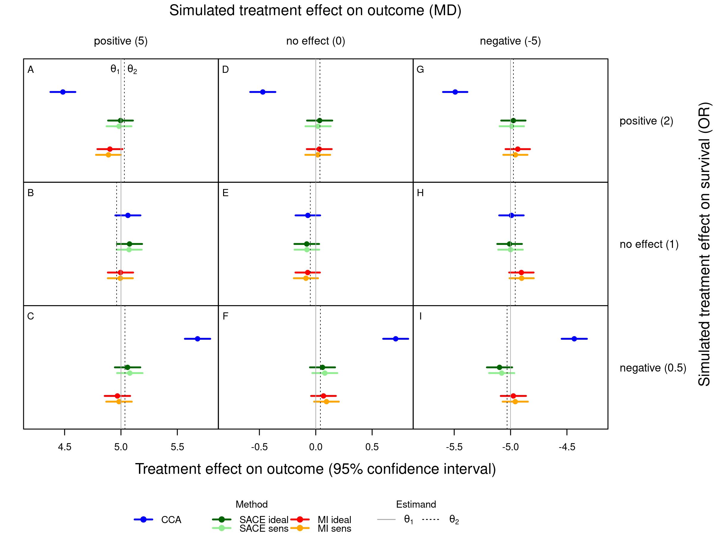
Figure 1: Average treatment effect estimates with 95 % Wald confidence intervals for each scenario (A–I) and method. For the SACE estimator and for multiple imputation, the average estimates from ideal analyses using all covariates (green and red) are shown together with those from the sensitivity analyses where the covariate head circumference was omitted (light green and orange). The scenarios are arranged with the treatment effect on survival in rows and the treatment effect on the outcome in columns. The vertical lines indicate the estimands, i.e., the treatment effect on the outcome used in the simulation, $\theta_{1}$ (solid black line), and the SACE derived from observed and counterfactual data, $\theta_{2}$ (dashed gray line). Note the different x-axis scales for the three columns (with different simulated treatment effects on outcome).

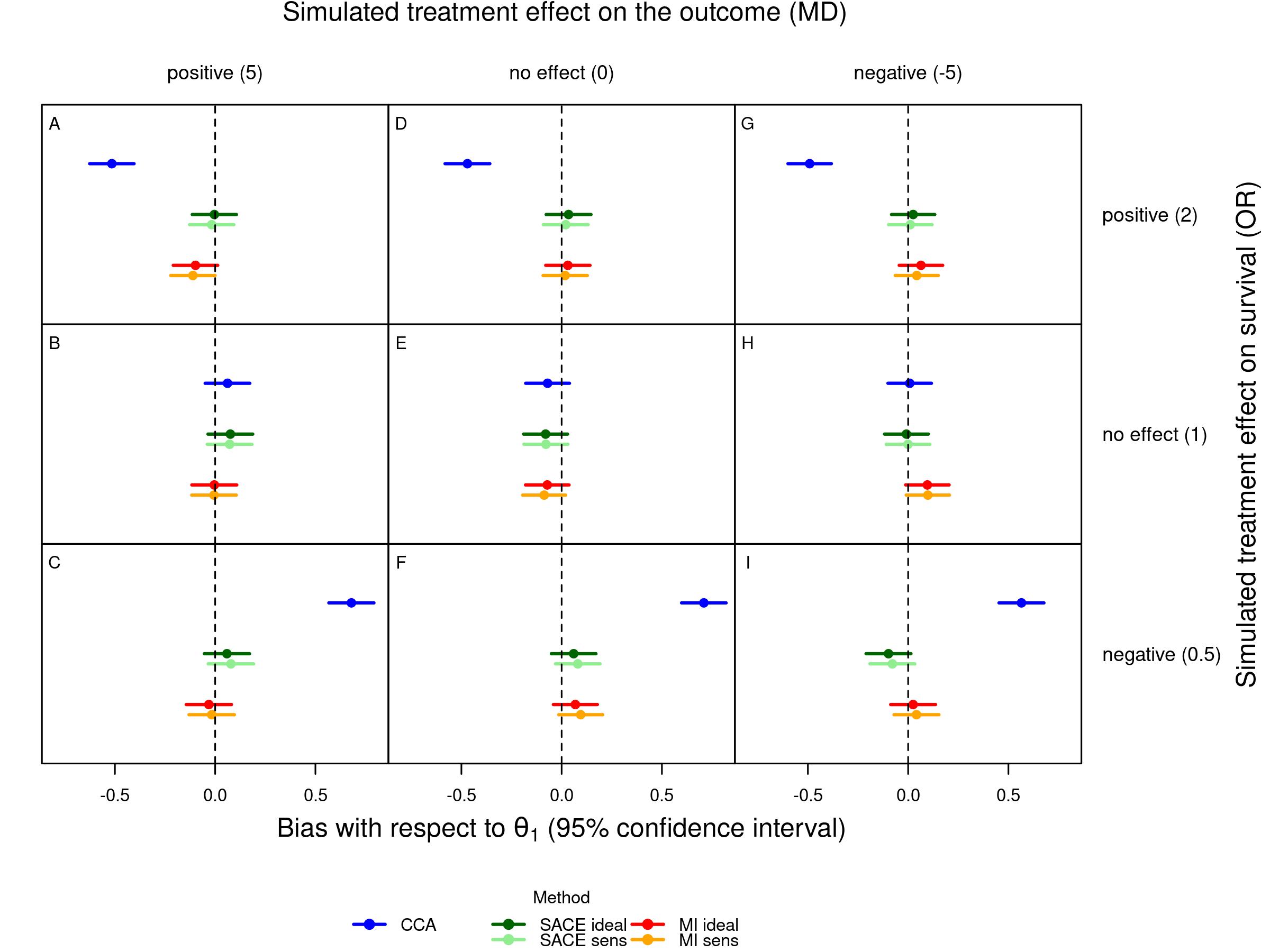
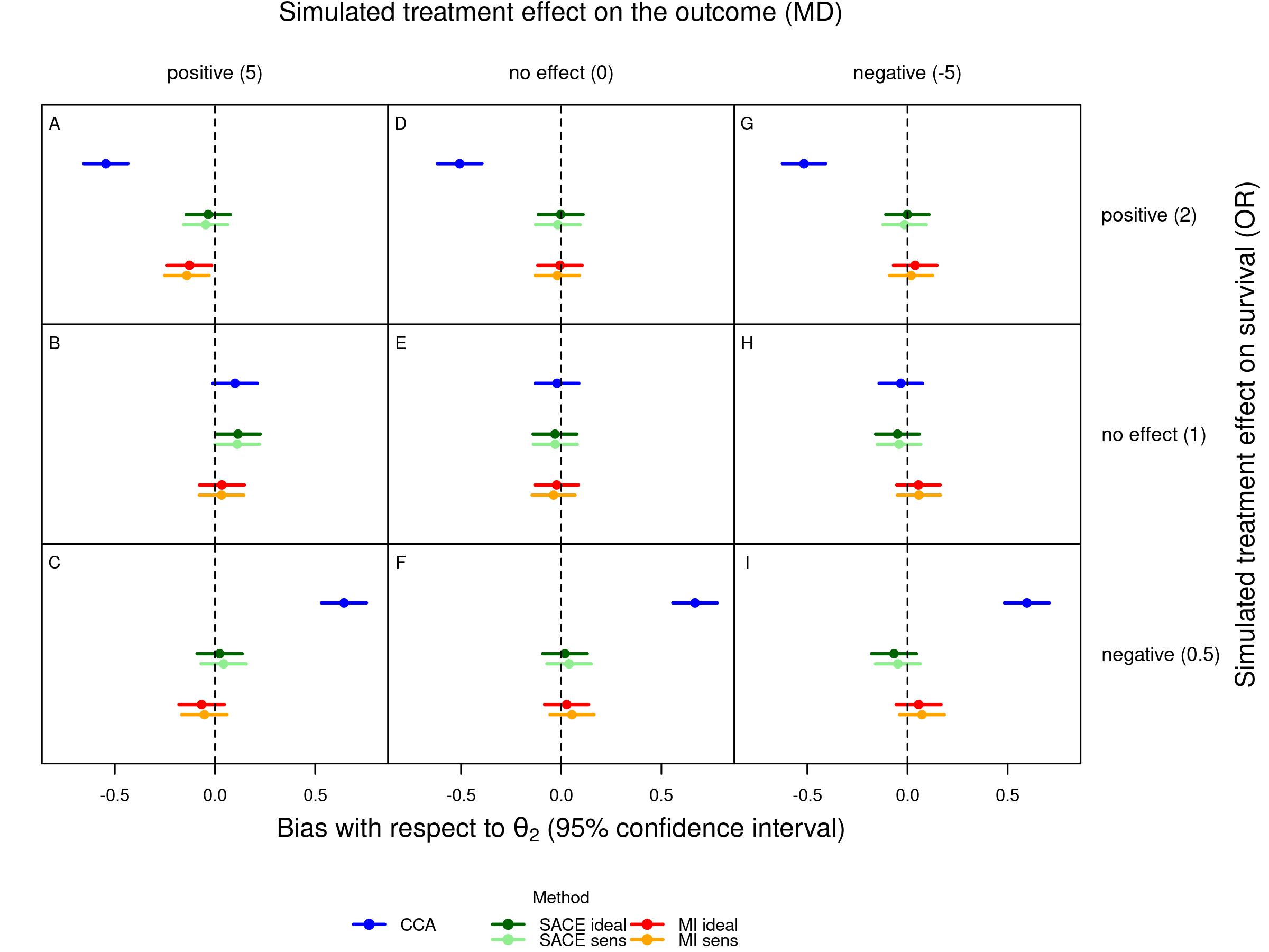
Figure 2: Average bias for each scenario (A–I) and method with regard to the treatment effect on the outcome used in the simulation, $\theta_{1}$ (top panels) and with regard to the SACE derived from observed and counterfactual data, $\theta_{2}$ (bottom panels). Bias is shown with 95 % Monte Carlo confidence interval. For the SACE estimator and for multiple imputation, the bias of ideal analyses using all covariates (green and red) is shown together with the bias of the sensitivity analyses where the covariate head circumference was omitted (light green and orange). The scenarios are arranged with the treatment effect on survival in rows and the treatment effect on the outcome in columns. The dashed vertical lines indicate no bias.

Table 4: Average bias regarding $\theta_{1}$ and $\theta_{2}$ depending on the treatment effect on survival (rows) and the method of analysis (columns).

Estimand	Treat. eff. survival (OR)	CCA	SACE ideal	SACE sensitivity	MI ideal	MI sensitivity
$\theta_{1}$	2	$-$0.4920	0.0185	0.0047	$-$0.0010	$-$0.0168
$\theta_{1}$	0	$-$0.0003	$-$0.0042	$-$0.0023	0.0067	0.0018
$\theta_{1}$	0.5	0.6512	0.0069	0.0268	0.0206	0.0398
$\hat{\theta_{2}}$	2	$-$0.5226	$-$0.0121	$-$0.0259	$-$0.0316	$-$0.0474
$\hat{\theta_{2}}$	0	0.0153	0.0113	0.0133	0.0222	0.0173
$\hat{\theta_{2}}$	0.5	0.6359	$-$0.0084	0.0115	0.0053	0.0245

3.3 Mean squared error

The top part of Figure 3 shows the average MSE for each scenario and method with regard to $\theta_{1}$, with the 95 % Monte Carlo confidence interval. Likewise, the bottom part of Figure 3 shows the average MSE with regard to $\theta_{2}$. The average MSE did not depend on the treatment effect on the outcome, which can be seen from the very similar patterns in all three columns of Figure 3, but it depended on the treatment effect on survival and on the method of analysis (rows and colors in Figure 3). As a consequence of the bias which was largest for complete case analysis, this method also had the largest average MSE of all methods in the presence of treatment effects on survival. The average MSE was similar and relatively small for all methods (and types of analyses) in scenarios without a treatment effect on survival (B, E, H), and largest in scenarios where Epo reduced survival compared to placebo (C, F, I, bottom rows of both parts of Figure 3). The latter is again a consequence of the larger mortality in these scenarios (Table 3), which also resulted in larger bias. Moreover, it is interesting to note that the average MSE was particularly large in scenarios C and I, with a treatment effect on the outcome (in addition to the negative treatment effect on survival), where a larger variance of the treatment effect estimate may have contributed to the MSE. As for bias, the differences in average MSE between the sensitivity analyses and the corresponding ideal analyses were relatively small.

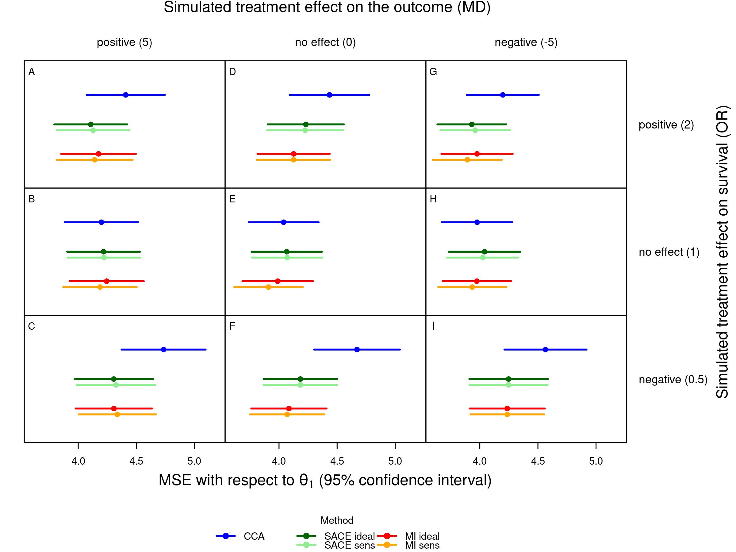
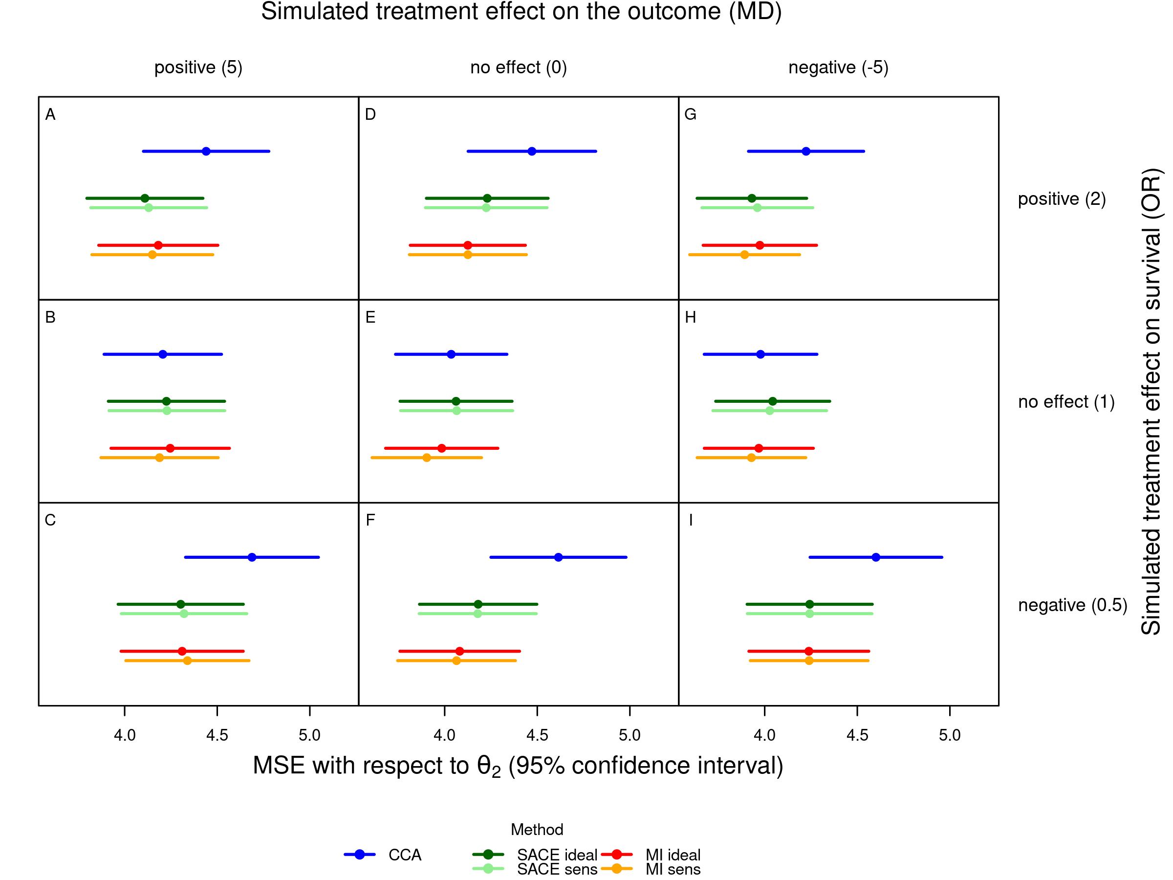
Figure 3: Average mean squared error (MSE) for each scenario (A–I) and method with regard to the treatment effect on the outcome used in the simulation, $\theta_{1}$ (top panels) and with regard to the SACE derived from observed and counterfactual data, $\theta_{2}$ (bottom panels). MSE is shown with 95 % Monte Carlo confidence interval. For the SACE estimator and for multiple imputation, the MSE of ideal analyses using all covariates (green and red) is shown together with the MSE of the sensitivity analyses where the covariate head circumference was omitted (light green and orange). The scenarios are arranged with the treatment effect on survival in rows and the treatment effect on the outcome in columns.

3.4 Coverage

The top part of Figure 4 shows the coverage for each scenario and method with regard to $\theta_{1}$, with the 95 % Monte Carlo confidence interval. Likewise, the bottom part of Figure 4 shows the coverage with regard to $\theta_{2}$. Tang et al., (2005) suggested that coverage can be expected to lie within the interval of the nominal coverage probability $\pm$ standard error, which is the standard error of a proportion, i.e., $\sqrt{\frac{p(1-p)}{n}}$, here $\sqrt{\frac{0.95\cdot 0.05}{1300}}$, and that values below this interval can be interpreted as under-coverage and values above as over-coverage. In the context of our simulation study, under- and over-coverage mean that the corresponding estimand is captured less and more often, respectively. Accordingly, the acceptable coverage range is 0.938 to 0.962 in our case, which is shown in Figure 4 (dotted vertical lines). Similarly, we can check whether the nominal confidence-level of 0.95 is included in the observed 95 % Monte Carlo confidence intervals for coverage. Both conditions are met with respect to both estimands in most cases. Exceptions are (1) complete case analysis with regard to $\theta_{1}$ in scenario C and with regard to $\theta_{2}$ in scenario D, where the point estimate for coverage lies below the acceptable range and the 95 % CI for coverage lies entirely below 0.95, indicating under-coverage and (2) the SACE estimator (ideal analysis) in scenario H with regard to $\theta_{1}$ and $\theta_{2}$, where the point estimate for coverage lies above the acceptable range and the 95 % CI for coverage lies entirely above 0.95, indicating over-coverage. Again as a consequence of the bias of complete case analysis, this method has a lower coverage than the other methods in the presence of treatment effects on survival. As for bias and MSE, the differences in coverage between the sensitivity analyses and the ideal analyses were relatively small, but the largest differences were observed for the two types of analyses using multiple imputation, in particular in scenarios without a treatment effect on the outcome.

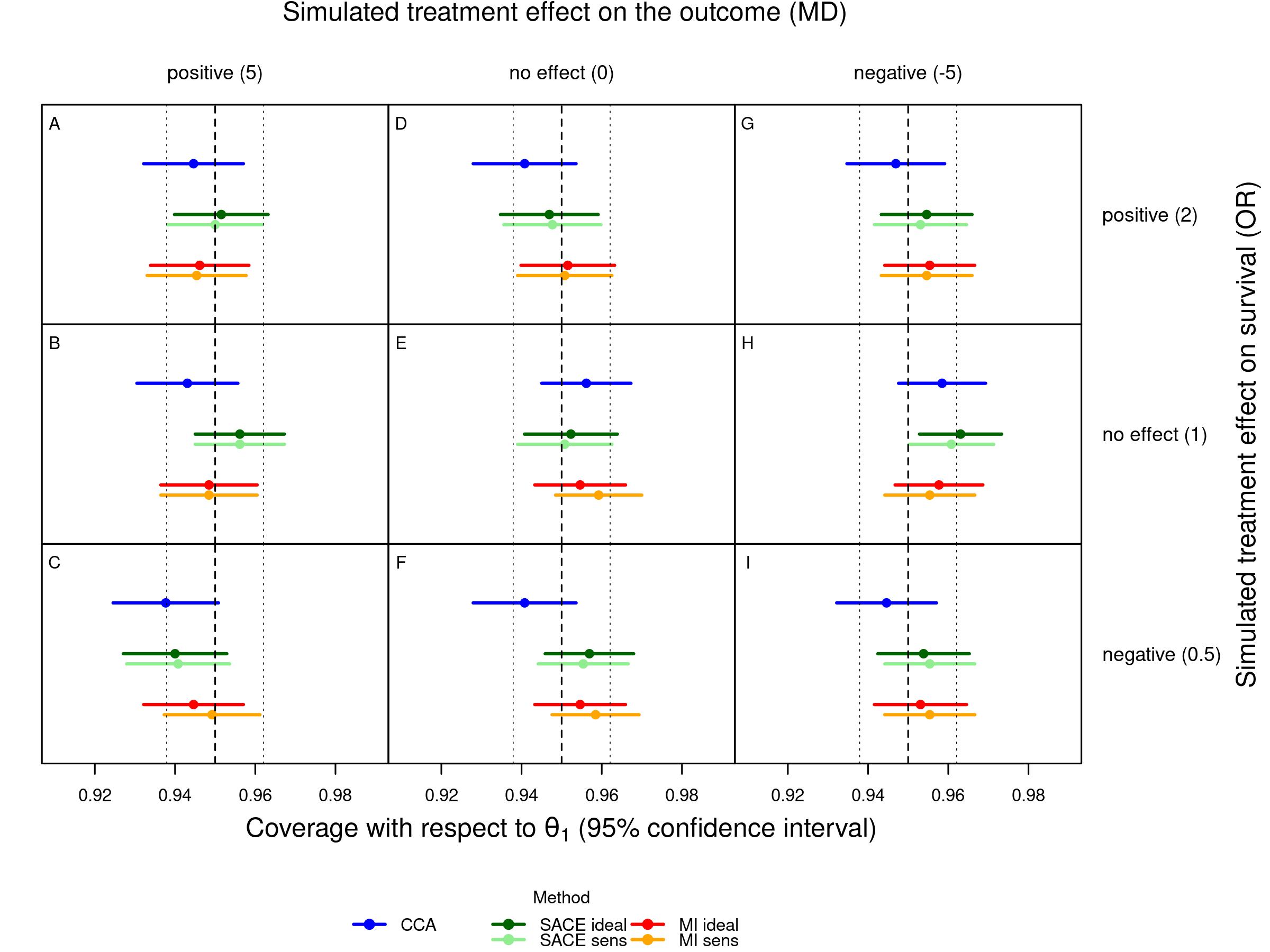
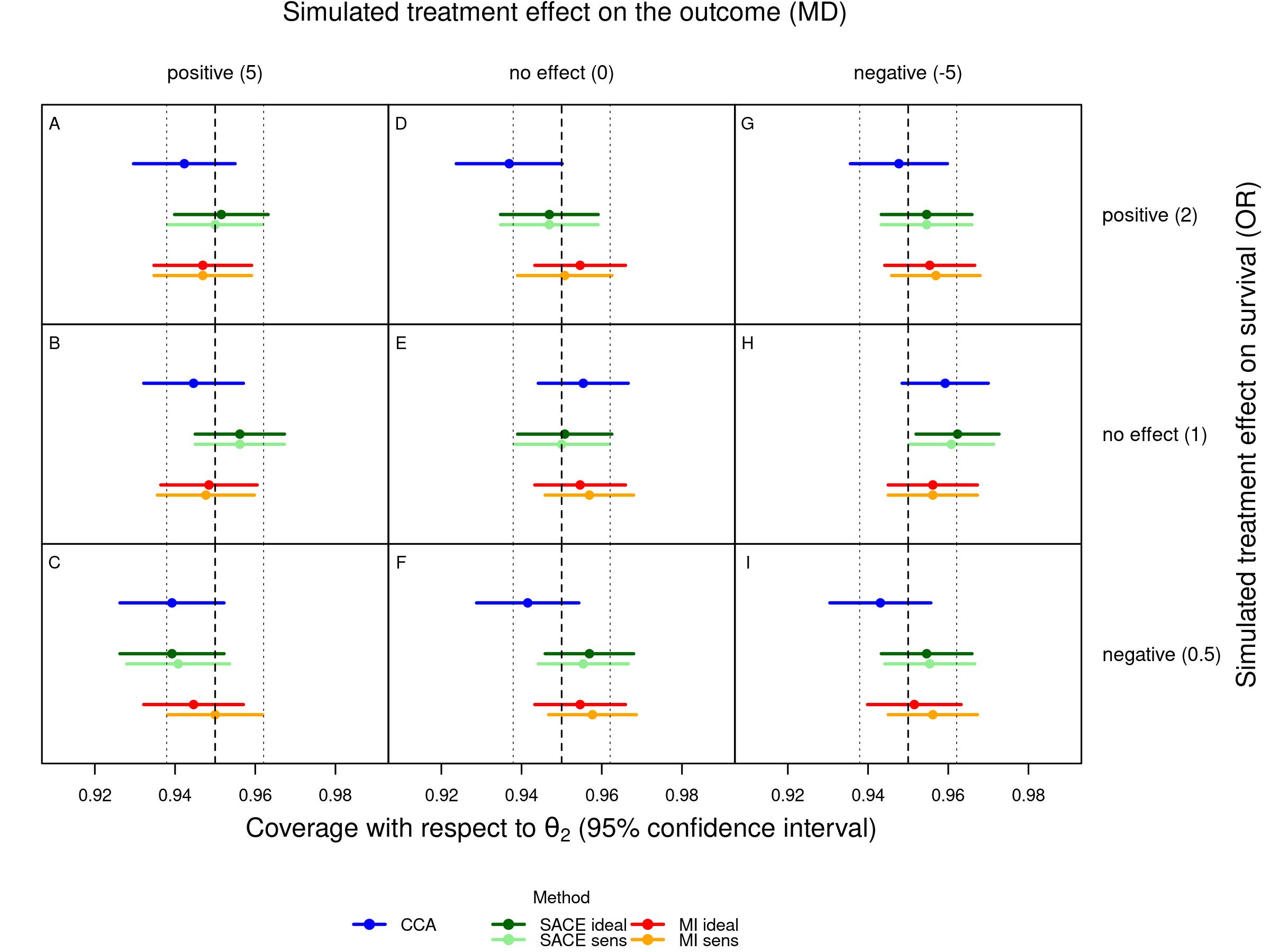
Figure 4: Coverage for each scenario (A–I) and method with regard to the treatment effect on the outcome used in the simulation, $\theta_{1}$ (top panels) and with regard to the SACE derived from observed and counterfactual data, $\theta_{2}$ (bottom panels). Coverage is shown with 95 % Monte Carlo confidence interval. For the SACE estimator and for multiple imputation, the coverage of ideal analyses using all covariates (green and red) is shown together with the coverage of the sensitivity analyses where the covariate head circumference was omitted (light green and orange). The scenarios are arranged with the treatment effect on survival in rows and the treatment effect on the outcome in columns. The dashed vertical lines indicate a coverage of 0.95, the dotted vertical lines indicate the acceptable coverage range (0.938 to 0.962).

4 Discussion

We performed a simulation study to compare treatment effect estimates by complete case analysis, an analysis after multiple imputation of the missing values and the SACE estimator proposed by Hayden et al., (2005). While complete case analysis does not target a causal estimand and is known to be biased in most cases, the other two approaches target a hypothetical and a principal stratum estimand, both of which are possible options when a continuous outcome is truncated by death. Not surprisingly, our results reveal the bias regarding the treatment effect on the outcome when using complete case analysis in the scenarios with a treatment effect on survival, even in the absence of a treatment effect on the outcome. A bias towards smaller or more negative treatment effects was found when treatment with Epo improved survival compared to Placebo (scenarios A, D, G, top rows of Figures 1 and 2), which can be explained by the survival of less healthy or less viable patients (e.g., preterm infants with lower gestational age, also called "frail mortality benefiters" by Colantuoni et al.,, 2018) under treatment compared to placebo. In contrast, a bias towards larger or less negative treatment effects was found when treatment with Epo reduced survival compared to Placebo (scenarios C, F, I, bottom rows of Figures 1 and 2), which can be explained by the death of more frail patients under treatment compared to placebo, which results in a treatment group with improved outcome. Both alternative approaches to complete case analysis, although targeting different estimands, efficiently reduced the bias compared to complete case analysis and led to similar estimates of the treatment effect. The SACE estimator used covariate information to reduce the analysis data set of a trial to the principal stratum of those who would have survived under both treatments. Multiple imputation used covariate information to substitute the outcome measurements truncated by death. Further, we showed that results of the SACE estimator were robust to a violation of the "explainable nonrandom survival" assumption due to omission of one covariate (head circumference at birth) in the analysis although it was used to generate the data.

Our results confirm and illustrate that complete case analysis is not a favorable option when outcomes are truncated by death, unless a treatment effect on survival can be virtually ruled out. However, the question remains whether the SACE as a principal stratum estimand or a hypothetical estimand (ignoring death) are more meaningful in this situation, or whether even both approaches have their justification. On the one hand, the relevance of the hypothetical estimand, the causal effect of the treatment on the outcome in the absence of mortality, is questioned because death could not be avoided by design in a future trial on preterm infants (while this may well be possible for other intercurrent events). On the other hand, principal stratum estimands are controversial. While they have been advocated by Frangakis and Rubin, (2002), have been viewed as the only sensible estimand when outcomes are truncated by death (Rubin,, 2006; VanderWeele,, 2011), and have seemingly taken a role in drug development (Akacha et al.,, 2017; Qu et al.,, 2021; Bornkamp et al.,, 2021), they have been criticised for the untestable assumptions required for their estimation and because they refer to a subset of the population that is not observable and may not even exist (Pearl,, 2011; Dawid and Didelez,, 2012; Stensrud et al.,, 2022). Stensrud et al., (2022) suggested “conditional separable effects” as alternative estimands to unravel treatment effects on a posttreatment variable such as death and treatment effects on an outcome of interest. This is certainly an elegant alternative to principal stratum estimands, in particular for oncology trials using chemotherapy with two components, as in the example given in their article. The controversy with regard to principal stratum estimands may be seen as an argument in favour of a hypothetical estimand. However, because both estimands have their clear shortcomings, we find it hard to clearly prefer one above the other. We therefore recommend to report both and to discuss the differences in interpretation. In the future, it will be very interesting to see how alternatives like “conditional separable effects” (Stensrud et al.,, 2022) will be taken up by trialists and biostatisticians in pharmaceutical and academic clinical research.

Regarding the observability of principal strata, an interesting approach was used by Qu et al., (2023). They argued that the potential outcomes of patients under both treatments can be observed in a cross-over trial when carry-over and period effects can be excluded. Hence, they used a 2$\times$2 cross-over trial to evaluate commonly used assumptions to estimate principal stratum effects, including monotonicity, principal ignorability, and cross-world assumptions of principal ignorability and principal strata independence. This set of assumptions also covers the assumptions made by Hayden et al., (2005). On the one hand, and in line with our assessment for the EpoRepair trial, they found that the monotonicity assumption did not hold well for two principal stratum variables. On the other hand, they found that “cross-world principal ignorability” and “cross-world principal stratum independence conditional on baseline covariates”, which they defined as two components of “explainable nonrandom survival” required by Hayden et al., (2005), seemed reasonable.

Of course, we could have used other methods than the one suggested by Hayden et al., (2005) to estimate the SACE. We chose this method because it neither assumes monotonicity nor exclusion restriction, which we both found unrealistic for the EpoRepair trial. In fact, in the context of the SACE in an RCT, monotonicity may be always questionable because if one treatment is believed to benefit survival a priori, a clinical trial would be unethical (Wang et al.,, 2017). However, avoiding monotonicity and exclusion restriction comes at the cost of making the “explainable nonrandom survival” assumption. As other cross-world assumptions, it is untestable using observed data, as it involves both potential outcomes of patients. Due to the simulation of both potential outcomes for each patient and subsequent ideal analysis using all covariates used in the simulation to model the survival probabilities, we created a situation in which the assumption was met. Further, we showed that results of the SACE estimator were robust to violation of the the "explainable nonrandom survival" assumption due to omission of one covariate (head circumference at birth) in the analysis, suggesting that some degree of violation may be acceptable in practice. Of note, the situation is not unlike that for methods to adjust for confounding such as propensity score weighting, which require that no unexplained confounders exist to be unbiased, and this assumption is also untestable. In both situations, however, subject matter expertise can be used to ensure that the most important covariates/confounders are measured and used in the analysis. Further, the use of a cross-over trial to assess several assumptions of principal stratification methods by Qu et al., (2023) suggested that specifically the assumptions made by Hayden et al., (2005) may not be unreasonable. Other advantages of this specific SACE estimator are the actual estimation of the SACE together with a confidence interval and its relatively convenient applicability. Of course, which assumptions are more or less realistic for certain RCTs should be assessed in each case. In the context of other trials, other methods may be a better choice. For example, the monotonicity assumption may be realistic in certain situations and can then be used to identify the strata-specific effects. Examples may be found in Lipkovich et al., (2022) and references therein.

Strengths of our simulation study are that we have written and made public a simulation study protocol in advance, and that we are comparing established methods, none of which we developed ourselves. A need for such neutral comparison studies has been identified, as studies comparing an own new method with existing methods are often overly optimistic with respect to the performance of the new method (Boulesteix et al.,, 2013; Pawel et al.,, 2023). A limitation of our simulation study is that we did not specifically assess situations in which the SACE ($\theta_{2}$) would differ from the causal effect of the treatment on the outcome in the absence of mortality ($\theta_{1}$). In fact, $\theta_{2}$ and $\theta_{1}$ were relatively similar in all scenarios, and as a consequence, the bias of the SACE estimator with regard to $\theta_{2}$ was only minimally smaller than the corresponding bias of the analysis using multiple imputation and vice versa. Simulation of scenarios in which these estimands differ may require a data generating mechanism that involves interactions between treatment and covariates regarding the outcome, when some of these covariates are also related to survival.

In clinical trials with functional outcomes truncated by death, in particular if mortality is inherent to the population studied, we believe that the SACE has a role. In contrast to other intercurrent events, death in such populations is impossible to avoid (by trial design), which makes a hypothetical estimand less meaningful. Some degree of violation of the required assumptions, in case of the SACE estimator of Hayden et al., (2005) the “explainable nonrandom survival” assumption, is almost certain, as it may be true for the assumptions of most methods. However, given that the most important covariates associated with survival are known and used in the analysis, this shortcoming may be acceptable. Further, several estimands may be used in parallel, e.g., one for the primary analysis and another for a supplementary analysis, as suggested in other contexts (e.g., the tripartite framework Akacha et al.,, 2017; Qu et al.,, 2021). In future studies we believe that it would be valuable to further explore the potential of simulation studies and crossover trials to evaluate the principal stratum approach and related assumptions.

Conflict of Interest

The authors have declared no conflict of interest in relation to this study. SW is co-founder of Neopredix, a spin-off company of the University of Basel

Data availability

Code to reproduce the calculations in this manuscript is available at https://osf.io/bf9ht

References

References

- Akacha et al., (2017) Akacha, M., Bretz, F., and Ruberg, S. (2017). Estimands in clinical trials–broadening the perspective. Statistics in Medicine, 36(1):5–19.
- Angrist et al., (1996) Angrist, J. D., Imbens, G. W., and Rubin, D. B. (1996). Identification of causal effects using instrumental variables. Journal of the American Statistical Association, 91(434):444–455.
- Bell et al., (2014) Bell, M. L., Fiero, M., Horton, N. J., and Hsu, C.-H. (2014). Handling missing data in RCTs; a review of the top medical journals. BMC Medical Research Methodology, 14(1):1–8.
- Bornkamp et al., (2021) Bornkamp, B., Rufibach, K., Lin, J., Liu, Y., Mehrotra, D. V., Roychoudhury, S., Schmidli, H., Shentu, Y., and Wolbers, M. (2021). Principal stratum strategy: potential role in drug development. Pharmaceutical Statistics, 20(4):737–751.
- Boulesteix et al., (2013) Boulesteix, A.-L., Lauer, S., and Eugster, M. J. (2013). A plea for neutral comparison studies in computational sciences. PLoS ONE, 8(4):e61562.
- Burton et al., (2006) Burton, A., Altman, D. G., Royston, P., and Holder, R. L. (2006). The design of simulation studies in medical statistics. Statistics in Medicine, 25(24):4279–4292.
- CHMP, (2010) CHMP (2010). Guideline on missing data in confirmatory clinical trials. Technical report, EMA/CPMP/EWP/1776/99 Rev. 1, Committee for Medicinal Products for Human Use (CHMP).
- Colantuoni et al., (2018) Colantuoni, E., Scharfstein, D. O., Wang, C., Hashem, M. D., Leroux, A., Needham, D. M., and Girard, T. D. (2018). Statistical methods to compare functional outcomes in randomized controlled trials with high mortality. BMJ, 360.
- Dawid and Didelez, (2012) Dawid, P. and Didelez, V. (2012). " imagine a can opener"–the magic of principal stratum analysis. The International Journal of Biostatistics, 8(1).
- Frangakis and Rubin, (2002) Frangakis, C. E. and Rubin, D. B. (2002). Principal stratification in causal inference. Biometrics, 58(1):21–29.
- Groenwold et al., (2012) Groenwold, R. H., Donders, A. R. T., Roes, K. C., Harrell Jr, F. E., and Moons, K. G. (2012). Dealing with missing outcome data in randomized trials and observational studies. American Journal of Epidemiology, 175(3):210–217.
- Hayden et al., (2005) Hayden, D., Pauler, D. K., and Schoenfeld, D. (2005). An estimator for treatment comparisons among survivors in randomized trials. Biometrics, 61(1):305–310.
- Hernán and Robins, (2020) Hernán, M. and Robins, J. (2020). Causal Inference: What If. BocaRaton: Chapman & Hall/CRC.
- Honaker et al., (2011) Honaker, J., King, G., and Blackwell, M. (2011). Amelia II: A program for missing data. Journal of Statistical Software, 45(7):1–47.
- ICH E9, (1998) ICH E9 (1998). Statistical principles for clinical trials. Technical report, CPMP/ICH/363/96. https://www.ema.europa.eu/en/ich-e9-statistical-principles-clinical-trials-scientific-guideline.
- ICH E9 , 2020 (R1) ICH E9 (R1) (2020). Addendum on estimands and sensitivity analysis in clinical trials to the guideline on statistical principles for clinical trials. Technical Report Step 5 (17 February 2020), EMA/CHMP/ICH/436221/2017. https://www.ema.europa.eu/en/documents/scientific-guideline/ich-e9-r1-addendum-estimands-sensitivity-analysis-clinical-trials-guideline-statistical-principles_en.pdf.
- Imbens and Rubin, (2015) Imbens, G. W. and Rubin, D. B. (2015). Causal inference in statistics, social, and biomedical sciences. Cambridge University Press.
- Kurland et al., (2009) Kurland, B. F., Johnson, L. L., Egleston, B. L., and Diehr, P. H. (2009). Longitudinal Data with Follow-up Truncated by Death: Match the Analysis Method to Research Aims. Statistical Science, 24(2):211–222.
- Largo et al., (1989) Largo, R., Pfister, D., Molinari, L., Kundu, S., Lipp, A., and Due, G. (1989). Significance of prenatal, perinatal and postnatal factors in the development of aga preterm infants at five to seven years. Developmental Medicine & Child Neurology, 31(4):440–456.
- Lipkovich et al., (2022) Lipkovich, I., Ratitch, B., Qu, Y., Zhang, X., Shan, M., and Mallinckrodt, C. (2022). Using principal stratification in analysis of clinical trials. Statistics in Medicine, 41(19):3837–3877.
- Morris et al., (2019) Morris, T. P., White, I. R., and Crowther, M. J. (2019). Using simulation studies to evaluate statistical methods. Statistics in Medicine, 38(11):2074–2102.
- Pawel et al., (2023) Pawel, S., Kook, L., and Reeve, K. (2023). Pitfalls and potentials in simulation studies: Questionable research practices in comparative simulation studies allow for spurious claims of superiority of any method. Biometrical Journal.
- Pearl, (2011) Pearl, J. (2011). Principal stratification–a goal or a tool? The international journal of biostatistics, 7(1):1–13.
- Qu et al., (2023) Qu, Y., Lipkovich, I., and Ruberg, S. J. (2023). Assessing the commonly used assumptions in estimating the principal causal effect in clinical trials. Statistics in Biopharmaceutical Research, 15(4):812–819.
- Qu et al., (2021) Qu, Y., Luo, J., and Ruberg, S. J. (2021). Implementation of tripartite estimands using adherence causal estimators under the causal inference framework. Pharmaceutical Statistics, 20(1):55–67.
- Robins, (1986) Robins, J. (1986). A new approach to causal inference in mortality studies with a sustained exposure period—application to control of the healthy worker survivor effect. Mathematical Modelling, 7(9-12):1393–1512.
- Robins, (1998) Robins, J. M. (1998). Correction for non-compliance in equivalence trials. Statistics in Medicine, 17(3):269–302.
- Rubin, (1980) Rubin, D. B. (1980). Randomization analysis of experimental data: The Fisher randomization test comment. Journal of the American Statistical Association, 75(371):591–593.
- Rubin, (1987) Rubin, D. B. (1987). Multiple imputation for nonresponse in surveys. John Wiley & Sons, Inc., New York, 1 edition. 258 pages.
- Rubin, (2006) Rubin, D. B. (2006). Causal inference through potential outcomes and principal stratification: application to studies with “censoring” due to death. Statistical Science, 21(3):299–309.
- Rüegger et al., (2015) Rüegger, C. M., Hagmann, C. F., Bührer, C., Held, L., Bucher, H. U., Wellmann, S., EpoRepair Investigators, et al. (2015). Erythropoietin for the repair of cerebral injury in very preterm infants (EpoRepair). Neonatology, 108(3):198–204.
- Stensrud et al., (2022) Stensrud, M. J., Robins, J. M., Sarveta, A., Tchetgen, E. J. T., and Young, J. G. (2022). Conditional separable effects. Journal of the American Statistical Association.
- Tang et al., (2005) Tang, L., Song, J., Belin, T. R., and Unützer, J. (2005). A comparison of imputation methods in a longitudinal randomized clinical trial. Statistics in Medicine, 24(14):2111–2128.
- van Buuren and Groothuis-Oudshoorn, (2011) van Buuren, S. and Groothuis-Oudshoorn, K. (2011). mice: Multivariate imputation by chained equations in R. Journal of Statistical Software, 45(3):1–67.
- VanderWeele, (2011) VanderWeele, T. J. (2011). Principal stratification–uses and limitations. The International Journal of Biostatistics, 7(1):0000102202155746791329.
- Vickers and Altman, (2013) Vickers, A. J. and Altman, D. G. (2013). Statistics notes: missing outcomes in randomised trials. BMJ, 346.
- Wang et al., (2017) Wang, L., Zhou, X.-H., and Richardson, T. S. (2017). Identification and estimation of causal effects with outcomes truncated by death. BIOMETRIKA, 104(3):597–612. Methodological.
- Wellmann et al., (2022) Wellmann, S., Hagmann, C. F., von Felten, S., Held, L., Klebermass-Schrehof, K., Truttmann, A. C., Knöpfli, C., Fauchère, J.-C., Bührer, C., Bucher, H. U., et al. (2022). Safety and short-term outcomes of high-dose erythropoietin in preterm infants with intraventricular hemorrhage: The EpoRepair randomized clinical trial. JAMA Network Open, 5(12):e2244744–e2244744.
- White et al., (2011) White, I. R., Horton, N. J., Carpenter, J., Pocock, S. J., et al. (2011). Strategy for intention to treat analysis in randomised trials with missing outcome data. BMJ, 342.