PSR B0943$+$10: Mode Switch, Polar Cap Geometry, and Orthogonally Polarized Radiation

Abstract

As one of the paradigm examples to probe into pulsar magnetospheric dynamics, PSR B0943$+$10 (J0946$+$0951) manifests representatively, showing mode switch, orthogonal polarization and subpulse drifting. Both integrated and single pulses are studied with the Five-hundred-meter Aperture Spherical radio Telescope (FAST). The mode switch phenomenon of this pulsar is studied using an eigen-mode searching method, based on parameter estimation. A phase space evolution for the pulsar’s mode switch shows a strange-attractor-like pattern. The radiative geometry is proposed by fitting polarization position angles with the rotating vector model. The pulsar pulse profile is then mapped to the sparking location on pulsar surface, and the differences between the main pulse’s and the precursor component’s radiative process may explain the X-ray’s synchronization with radio mode switch. Detailed single pulse studies on B0943$+$10’s orthogonally polarized radiation are presented, which may support for certain models of radiative transfer of polarized emission. B0943$+$10’s B and Q modes evolve differently with frequency and with proportions of orthogonal modes, which indicates possible magnetospheric changes during mode switch. An extra component is found in B mode, and it shows distinct polarization and modulation properties compared with main part of B mode pulse component. For Q mode pulse profile, the precursor and the main pulse components are orthogonally polarized, showing that the precursor component radiated farther from the pulsar could be radiated in O-mode (X-mode) if the main pulse originates from low altitude in X-mode (O-mode). The findings could impact significantly on pulsar electrodynamics and the radiative mechanism related.

1 Introduction

Pulsars are usually interpreted as highly magnetized rotating compact stars emitting pulse-like periodic signals. Their abundant radiation properties are closely related to some basic problems in pulsar physics, but are still poorly understood. PSR B0943$+$10 (J0946$+$0951) is a well-known pulsar rich in radiation phenomena. It is a typical mode-switching pulsar with two stable radiation modes showing distinct radiation phenomena. There exists a B (“Burst” or “Bright”) mode with organized simple sub-pulse drifting pattern and a Q (“Quiescent” or “Quiet”) mode with disorganized single pulses (e.g., Suleymanova et al., 1998; Deshpande & Rankin, 2001). Since its discovery in 1968 (Vitkevich et al., 1969), many radio observations have been carried out on B0943$+$10 (e.g., Suleymanova et al., 1998; Deshpande & Rankin, 1999; Backus et al., 2011; Bilous et al., 2014). Radio observations on B0943$+$10 are mostly made on relatively low frequencies (below 600MHz), because the source becomes dimmer quickly when frequency increases (Deshpande & Rankin, 1999) (also see Arecibo L band observation of B0943$+$10 in Weisberg et al. (1999)).

Suleymanova et al. (1998) and Deshpande & Rankin (2001) studied B0943$+$10’s orthogonal polarization modes (OPMs). They introduced a primary polarization mode (PPM), a secondary polarization mode (SPM) and a unpolarized mode (UP) (see Figure 16 in Deshpande & Rankin (2001)) to describe its polarized pulse sequence. PPM and SPM are orthogonally polarized with polarization position angle curves having a 90^∘ departure. It was found that B0943$+$10’s radiation modes have different proportions of PPM and SPM at 103MHz (Suleymanova et al., 1998): B mode is PPM dominated (90%) while Q mode is SPM dominated (59%), leading to Q mode profile’s lower linear polarization fraction. Moreover, Deshpande & Rankin (2001) applied a polarization-mode separation technique to B0943$+$10’s B mode profiles at 430MHz, and found that the yielded PPM and SPM appears opposite directions of circular polarization: PPM is left-hand circular (Stokes $V>0$) and SPM is right-hand circular (Stokes $V<0$). In the last 20 years, attentions are mostly paid on this pulsar’s sub-pulse drifting phenomena and profile evolution (e.g., Rankin & Suleymanova, 2006; Suleymanova & Rankin, 2009; Bilous et al., 2014; Suleymanova et al., 2021). We haven’t made new progress on B0943$+$10’s sub-pulse drifting, and this paper concentrates on mode switch and polarization properties.

Beside radio observations, X-ray observation of B0943$+$10 raises more questions. Hermsen et al. (2013) found that B0943$+$10 shows different ways of X-ray emission in different radio radiation modes: a thermal X-ray pulsation appears strong in Q mode, but weak in B mode. The reason of such relation between X-ray emission and modes remains largely unknown.

Now with the help of China’s Five-hundred-meter Aperture Spherical radio Telescope (FAST), more single pulses and polarization studies can be made on B0943$+$10, under FAST L band (1-1.5GHz). The paper is structured as follows. Firstly in Section 2, the basic information of our observations and data processing methods are presented, especially the eigen mode search algorithm. Section 3 shows the results of studies on B0943$+$10’s profile evolution and polarization properties. Some discussions on the results are presented in Section 4. The conclusion is given in Section 5.

2 Observation and data reduction

Four epochs of observation during May, 2022 to August, 2023 are used in this paper. All of them are made by FAST at small zenith angles ($<20^{\circ}$), with L-band 19-beam receiver (Jiang et al., 2020). The data is recorded under the frequency band 1000 MHz to 1500 MHz, and the band is divided into 4096 channels. The time resolution of the recording is 49.152$\mu$s. At the beginning of each observation, modulated signals from a noise diode were injected as a 100% linearly polarized source for polarimetric calibration. The data processing (including folding, RFI mitigation, calibration and timing) is done with software packages dspsr (van Straten & Bailes, 2011), psrchive (Hotan et al., 2004) and tempo2 (Hobbs et al., 2006).In this paper, we follow the PSR/IEEE convention for the definition of Stokes parameters (van Straten et al., 2010). We use a Bayesian method to fit for the rotation measure (RM) of Faraday rotation (Luo et al., 2020). For single pulses, baselines of system noise are fitted with linear functions and then subtracted. Table 1 shows basic information of 4 epochs and the updated RM values using FAST data.

Table 1: SOME PARAMETERS OF PSR B0943$+$10

Observation date (UTC)	Time length (s)	RM (m-2)
20220517……………….	7335	16.1$\pm 0.2$
20220902……………….	3000	18.4$\pm 0.3$
20230816……………….	3280	20.2$\pm 0.3$
20230827……………….	2720	19.2$\pm 0.3$

2.1 Eigen mode search

2.1.1 Basic algorithm

Take 20220902 epoch for example. The waterfall plot of all 20220902 observation’s single pulses are given in Figure 2. There is a mode switch occurred around $N\sim 1100$.

To make a clear description of the mode switches and other profile evolution processes, Hao et al. (2023, submitted) put forward an eigen mode searching method. We extend the method from only calculating eigen modes of $I$ to calculating eigen modes of polarized profiles $I$, $L$ and $V$ together. Any sub-integrations (noted with $p_{ij}$, $i$-th sub-integration at phase $j$) could be linearly decomposed into some eigen modes ($f_{j}$ and $g_{j}$, take two modes for example) together with a certain amount of noise ($n_{ij}$):

$$p_{ij}=\alpha_{i}f_{j}+\beta_{i}g_{j}+n_{ij}$$ (1)

Here $\alpha_{i}$ and $\beta_{i}$ represent the mixture weights of eigen modes $f_{j}$ and $g_{j}$. Assuming $n_{ij}$ follows Gaussian distribution, the likelihood used to estimate the modes and the weights could be written in the form:

$$\Lambda=Ce^{-\dfrac{1}{2}\sum_{i}\sum_{j}\left(\dfrac{p_{ij}-\alpha_{i}f_{j}-\beta_{i}g_{j}}{\sigma_{ij}}\right)^{2}}$$ (2)

Here $\sigma_{ij}$ means the uncertainty of the sub-integration profile value at the $i$-th sub-integration profile’s $j$-th phase. The relations between the max estimated parameters are yielded from $\partial\Lambda/\partial\alpha_{i}=0$, $\partial\Lambda/\partial\beta_{i}=0$, $\partial\Lambda/\partial f_{i}=0$ and $\partial\Lambda/\partial g_{i}=0$:

$$\sum_{i}(p_{ij}-\alpha_{i}f_{j}-\beta_{i}g_{j})\dfrac{f_{j}}{\sigma_{ij}}=0$$ (3)

$$\sum_{i}(p_{ij}-\alpha_{i}f_{j}-\beta_{i}g_{j})\dfrac{g_{j}}{\sigma_{ij}}=0$$ (4)

$$\sum_{i}(p_{ij}-\alpha_{i}f_{j}-\beta_{i}g_{j})\dfrac{\alpha_{i}}{\sigma_{ij}}=0$$ (5)

$$\sum_{i}(p_{ij}-\alpha_{i}f_{j}-\beta_{i}g_{j})\dfrac{\beta_{i}}{\sigma_{ij}}=0$$ (6)

Equations above could be written in the form of matrices, and be used for iteration calculation of $f_{j}$, $g_{j}$, $\alpha_{i}$ and $\beta_{i}$:

$$\left(\begin{matrix}f_{j}^{\prime}\\ g_{j}^{\prime}\\ \end{matrix}\right)=\left(\begin{matrix}\sum_{i}\dfrac{\alpha_{i}^{2}}{\sigma_{ij}}&\sum_{i}\dfrac{\alpha_{i}\beta_{i}}{\sigma_{ij}}\\ \sum_{i}\dfrac{\alpha_{i}\beta_{i}}{\sigma_{ij}}&\sum_{i}\dfrac{\beta_{i}^{2}}{\sigma_{ij}}\\ \end{matrix}\right)^{-1}\left(\begin{matrix}\sum_{i}\dfrac{p_{ij}\alpha_{i}}{\sigma_{ij}^{2}}\\ \sum_{i}\dfrac{p_{ij}\beta_{i}}{\sigma_{ij}^{2}}\\ \end{matrix}\right)$$ (7)

$$\left(\begin{matrix}\alpha_{i}^{\prime}\\ \beta_{i}^{\prime}\\ \end{matrix}\right)=\left(\begin{matrix}\sum_{j}\dfrac{f_{j}^{2}}{\sigma_{ij}}&\sum_{j}\dfrac{f_{j}g_{j}}{\sigma_{ij}}\\ \sum_{j}\dfrac{f_{j}g_{j}}{\sigma_{ij}}&\sum_{j}\dfrac{g_{j}^{2}}{\sigma_{ij}}\\ \end{matrix}\right)^{-1}\left(\begin{matrix}\sum_{j}\dfrac{p_{ij}f_{j}}{\sigma_{ij}^{2}}\\ \sum_{j}\dfrac{p_{ij}g_{j}}{\sigma_{ij}^{2}}\\ \end{matrix}\right)$$ (8)

The sub-integration $p_{ij}$ is a “flatten” profile of $I$, $L$ and $V$: suppose the number of bins of profiles $I$, $L$ and $V$ is nbin, then the number of bins of $p_{ij}$ is $3\times$ nbin. The profiles of $I$, $L$ and $V$ are located at bin ranges of (0, nbin), (nbin, $2\times$ nbin) and ($2\times$ nbin, $3\times$ nbin) for $p_{ij}$.

The calculation begins by setting the number of eigen modes as 1 with random initial values of the mixture weight, and the results are ($f_{j}^{(1)}$, $\alpha_{i}^{(1)}$). When setting 2 eigen modes, $\alpha_{i}^{(1)}$ are set as the initial values of $\alpha_{i}^{(2)}$, and the initial values of $\beta_{i}^{(2)}$ are initialized randomly. In this way we can calculate 3 eigen modes, 4 eigen modes, and so on.

Practically, before decomposing the eigen modes, we align the pulse profiles of $I$, $L$ and $V$ to mitigate the sub-pulse drifting. The pulse profiles can be rotated using Fast Fourier Transformation (FFT):

$$\mathscr{F}^{-1}(\mathscr{F}(p)e^{i\omega\Delta t})=p(t+\Delta t)$$ (9)

The $\Delta t$ of two profiles $p_{1}$ and $p_{2}$ can be yielded below. The arguments of $\mathscr{F}(p_{1})$ and $\mathscr{F}(p_{2})$ could be written in the form:

$$\Phi_{1,k}=i\omega_{k}t$$ (10)

$$\Phi_{2,k}=i\omega_{k}(t+\Delta t)$$ (11)

The $\omega_{k}$ is just 0, 1, 2, … k … as is defined in FFT algorithm. So through fitting $\Phi_{2,k}-\Phi_{1,k}=\omega_{k}\Delta t$, we can get $\Delta t$ and use it to align profiles by Equation 9.

2.1.2 Special way to handle narrow peaks shifting in phase

During data reduction, we notice that there exists some narrow peaks (e.g. at $N\approx 560$ in Figure 2) shifting in phase in the pulse profiles of B0943$+$10, which might be caused by the existence of sub-pulse drifting. Due to the arbitrariness in phase-shifting, the narrow peaks are hard to be fitted using the basic algorithm described in Section 2.1.1, so a new step should be introduced after all components except those narrow shifting ones having been decomposed using the basic algorithm: calculate the residuals of basic algorithm results ($p_{ij}-(\alpha_{i}f_{j}+\beta_{i}g_{j}+\gamma_{i}h_{j}+...)$), align the narrow peaks in the residuals, and use the basic algorithm again to find the additional narrow component in the aligned residuals.

3 Results

The four FAST observation epochs’ integrated pulse profiles of PSR B0943$+$10 are shown in Figure 1. The profiles’ polarization position angle (PA) curves could be well fitted with Rotating Vector Model (RVM, Radhakrishnan & Cooke (1969)), and the details on the geometry will be discussed in Section 3.2. All pulse profiles’ phase $0$ is chosen where the fitting RVM curves are steepest, i.e. the $\phi=\phi_{0}$ point of Equation 13.

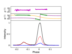
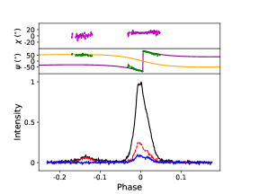
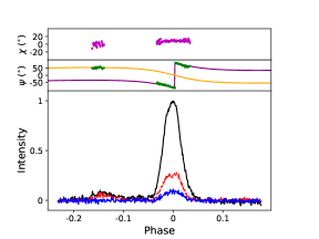
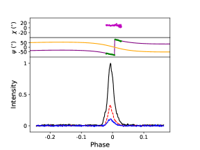
Figure 1: Integrated profiles of 20220517 (upper, left), 20220902 (upper, right), 20230816 (lower, left) and 20230827 (lower, right) observation epochs. Lower panel: black line - intensity ($I$), red line - linear polarization intensity ($L=\sqrt{Q^{2}+U^{2}}$), blue line - circular polarization intensity ($V$) (all normalized by maximum intensity); Upper panel: green dots - polarization position angle (PA, $\psi=0.5\arctan(U/Q)$), magenta dots - elliptical angel (EA, $\chi=0.5\arcsin(V/{\sqrt{U^{2}+Q^{2}+V^{2}}})$). Two RVM curves (purple and orange lines in the middle panels) with $90^{\circ}$ displacement are used to best fit the PA curves. The $\alpha$ and $\beta$ of the RVM curves are all same.

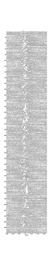
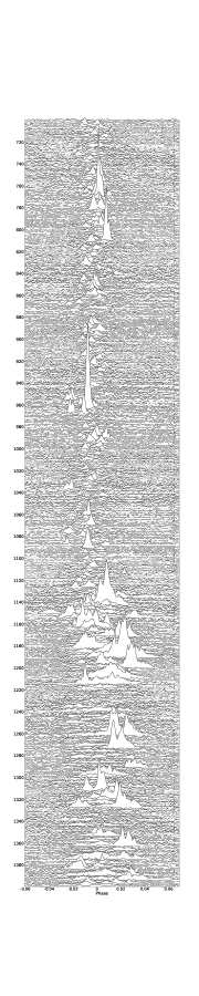
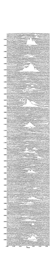
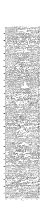
Figure 2: Waterfall plot of 2617 pulses. Horizontal axis: phase (0-1 for a period); vertical axis: number of pulses ($N$, top to bottom).

3.1 Modes and profiles’ evolution

3.1.1 20220517 observation: pure Q mode

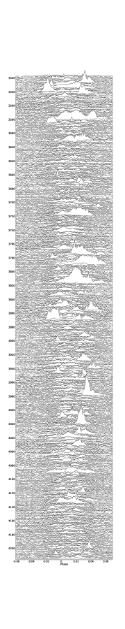
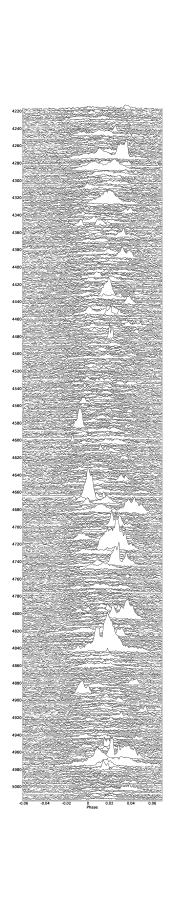
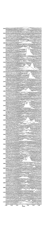
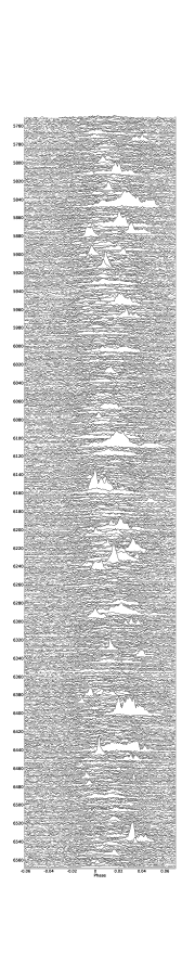
Figure 24: Waterfall plot of 6567 pulses in 20220517 observation (part 2). Horizontal axis: phase (0-1 for a period); vertical axis: number of pulses ($N$, top to bottom).

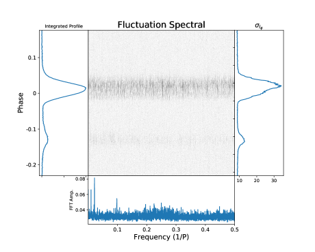
Figure 26: LRFS of 6567 pulses in 20220517 observation. The plots’ meanings are same as Figure 3.

The 20220517 profile in Figure 1 has a highly linearly polarized ($\sim 100$%) precursor component at about 0.14 phase earlier than the main component. This feature is consistent with B0943$+$10’s Q mode profile reported by other observations (e.g., Backus et al., 2010; Hermsen et al., 2013). Besides, the longitude-resolved fluctuation spectral (LRFS) of totally 6567 pulses in 20220517 observation is given in Figure 26 (Appendix B). There’s no periodic fluctuation in the pulse components, which is typical for B mode pulses (e.g., Deshpande & Rankin, 2001). Also no mode switch happens in the pulse sequence (shown in Figure 23 and Figure 24 in Appendix A) in 20220517 observation. All these facts indicating that pulses in 20220517 observation data are pure Q mode.

3.1.2 20230827 observation: pure B mode

The 20230827 profile in Figure 1 appears only one pulse component, and it is manifestly narrower than the Q mode pulse profile of 20220517 observation. Figure 3 (Appendix B) shows 20230827 pulses’ LRFS, where there is an FFT amplitude peak at about 0.47 cycle/P, only in the pulse phase range. This fluctuation frequency is consistent with results of former studies on B0943$+$10’s B mode (e.g., Deshpande & Rankin, 2001). Also no mode switch happens in the pulse sequence (shown in Appendix A Figure 25) in 20230827 observation. All these facts indicate that pulses in 20230827 observation data are pure B mode.

It’s worth noticing that in Figure 3 at phase $\phi\approx-0.025$, a distinct line appears in fluctuation spectral, and there is a peak of standard deviation of single pulses’ intensity. Such phenomena indicates a extra component in B mode pulses.

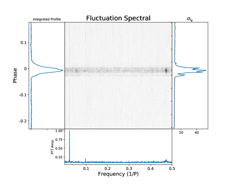
Figure 3: LRFS of 2358 pulses in 20230827 observation. The body show FFT amplitude of each phase and frequency. The left-hand panel shows the integrated profile of the observed pulses. The right-hand panel shows the standard deviation of single pulse intensity on every phase bins. The lower panel shows the integral spectra. A peak at 0.023 cycle/P appears not only in on-pulse phase range but also in off-pulse phase range, and it’s due to folding made with dspsr.

3.1.3 20220902 observation: B-to-Q switch

Figure 2 has clearly shown a mode switch from narrow pulses to wide pulses in 20220902 epoch. For a detailed study, 100 pulses are added together as a sub-integration every 5 pulses (e.g. 1-100, 6-105, …). Figure 4 presents 4 eigen modes calculated from the eigen mode search method described in Section 2.1. There are 3 basic-algorithm components and 1 narrow peak component, and their mixture weights are also shown.

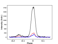
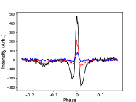
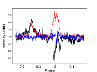
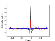
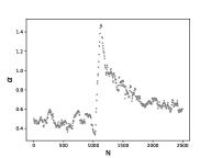
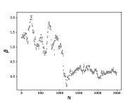
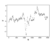
Figure 4: Upper 4 panels: 4 eigen profiles (marked 1 to 4 from left to right). The lines’ meanings are same as Figure 1. Lower 4 panels: mixture weights of 4 eigen modes versus pulse number ($N$) in full 20220902 pulse sequence.

Eigen mode 1 has a wide main pulse component and a precursor component with plus sign, mainly representing the radiation mode after mode switch ($N\gtrsim 1100$), which appears as a sudden jump in Eigen mode 1’s mixture weights versus pulse number. Eigen mode 2 has a narrow main pulse component and a minus-sign precursor component, indicating that in this mode the narrow main pulses are unlikely be accompanied by the precursor. The jumps in mixture weights of Eigen mode 2 also clearly reveal the mode switch. The quotient of first two eigen modes’s weights and a 2D plane shows their weights are shown in Figure 5, showing the distinct two modes and the mode switch process. It’s worth noting that the 2D phase space evolution in the right-hand sub-figure in Figure 5 appears like a strange attractor of a chaotic system. Eigen mode 3 shows a relation between main pulses’ $I$, $L$ and precursor components’ $I$, $L$: when the precursor becomes stronger in $I$ and $L$, the main component tends to have larger $L$ but smaller $I$. Eigen mode 4 is very narrow and sharp, representing some very strong pulses in the sub-pulse drifting sequence. The mixture weights of eigen mode 4 show a quasi-periodic oscillation before mode switch, which might correspond to the quasi-periodic appearance of strong pulses in the radiation mode. The period is about 200 pulses.

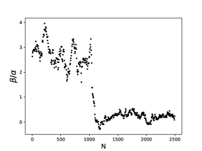
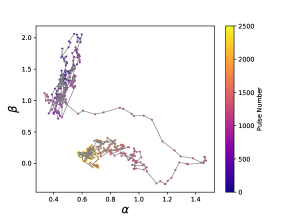
Figure 5: Left: The quotient of Eigen mode 1 and 2’s mixture weights. Right: Eigen mode 1’s mixture weights (horizontal axis) and Eigen mode 2’s mixture weights (vertical axis) shown in 2D plane. The colorbar is used to mark the pulses’ evolution on this $\alpha$-$\beta$ diagram with the pulse number’s increase. The pulse sequence begins at deep blue dots and ends at bright yellow dots.

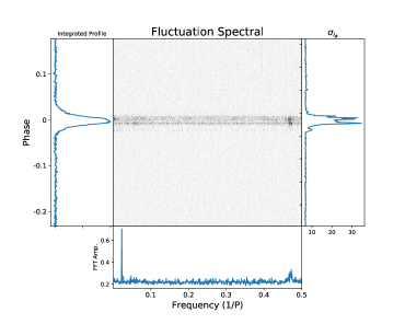
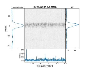
Figure 27: LRFS of 1128 first mode pulses (B, left), 1489 second mode pulses (Q, right) in 20220902 observation. The plots’ meanings are same as Figure 3.

The waterfall plot (Figure 2) and the eigen mode search results reveal that the mode switch takes place at $N\approx 1129$. Figure 6 shows the integrated profiles of the first mode ($N=$ 1 to 1128) and the second mode ($N=$ 1129 to 2617), where there is a highly linearly polarized precursor component in the profile of the second mode. And LRFSs of the two modes’ single pulses are shown in Figure 27 (Appendix B). The first mode’s FFT amplitude has a peak at about 0.47 cycle/P while the second dosen’t have. Comparing to results of 20220517 (Section 3.1.1) and 20230827 (Section 3.1.2), the conclusion is that the first mode is B mode and the second mode is Q mode. 20220902 observation contains a B-to-Q mode switch. The extra component at $\phi\approx-0.025$ also appears in Figure 27 in B mode.

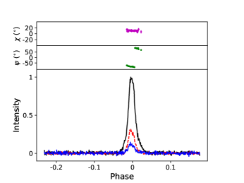
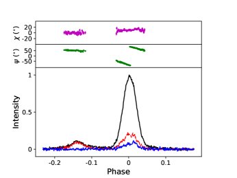
Figure 6: Integrated profiles of the first mode (B, left) and the second mode (Q, right) in 20220902 observation. Lines’ and dots’ meanings are same as Figure 1.

Knowing FAST’s system temperature ($T_{\text{sys}}$) and gain ($G$) (using data from Jiang et al. (2020)), the flux of the two modes could be estimated:

$$I_{\phi}=\dfrac{\text{SNR}\cdot T_{\text{sys}}}{G}\sqrt{\dfrac{\text{nbin}}{2\times\text{bandwidth}\times t_{\text{obs}}}}$$ (12)

The comparison of the two modes’ flux is shown in Figure 7. While Q mode being apparently dimmer under low frequencies (like Figure 1 in Backus et al. (2011), under 1-1.5GHz Q mode is almost as bright as B mode, indicating different frequency evolutions of the two modes.

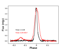
Figure 7: The comparison between B mode average profile’s (black line) and Q mode average profile’s (red line) flux under FAST L band, in 20220902 epoch.

3.1.4 20230816 observation: Q-to-B (or B’) switch

Figure 8 shows the waterfall plots for 20230816 observation. A mode switch takes place at $N\approx 1180$. We do the same algorithm on 20230816 pulse sequence as 20220902 observation. And the mode search results are shown in Figure 9 and Figure 10.

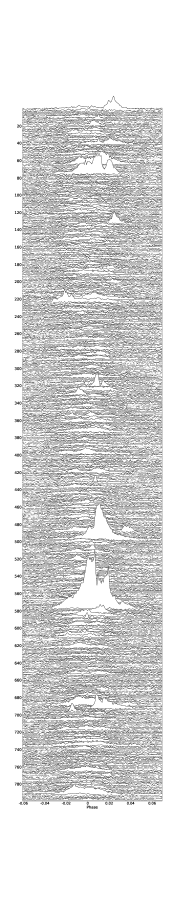
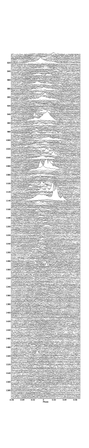
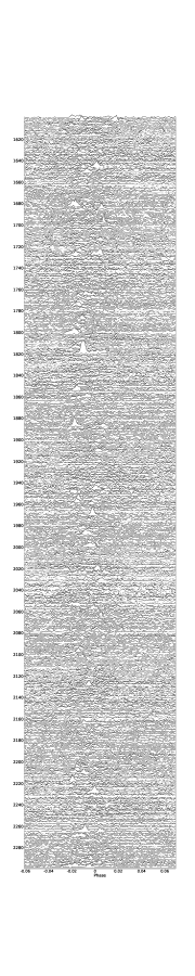
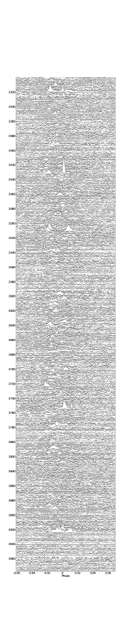
Figure 8: Waterfall plot of 2978 pulses in 20230816 observation. Horizontal axis: phase (0-1 for a period); vertical axis: number of pulses ($N$, top to bottom).

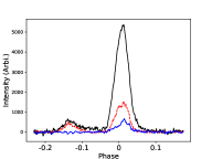
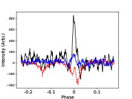
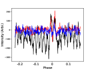
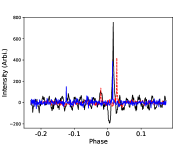
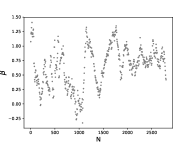
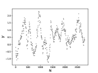
Figure 9: Upper 4 panels: 4 eigen profiles (marked 1 to 4 from left to right). The lines’ meanings are same as Figure 1. Lower 4 panels: mixture weights of 4 eigen modes versus pulse number ($N$) in full 20230816 pulse sequence.

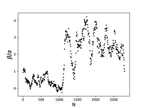
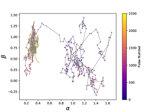
Figure 10: Left: The quotient of Eigen mode 1 and 2’s mixture weights. Right: Eigen mode 1’s mixture weights (horizontal axis) and Eigen mode 2’s mixture weights (vertical axis) shown in 2D plane. The colorbar is used to mark the pulses’ evolution on this $\alpha$-$\beta$ diagram with the pulse number’s increase.

Eigen mode 1 in 20230816 observation is like 20220902’s eigen mode 1, and its mixture weights show a jump around N $\sim 1100$, consistent with the mode switch. 20230816’s Eigen mode 2 is also narrow and with no precursor component. However, what’s apparently different with 20220902’s Eigen mode 2 is that 20230816’s Eigen mode 2 has linear polarization intensity $L<0$ within all main pulse component phases, which means that pulses with a larger weight of Eigen mode 2 tend to have smaller $L$.

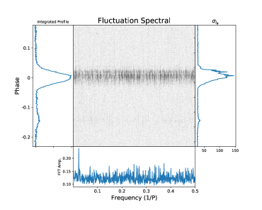
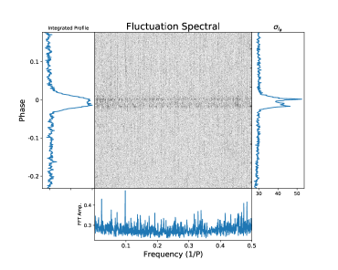
Figure 28: LRFS of 1179 first mode pulses (Q, left), 1798 second mode pulses (B’, right) in 20230816 observation. The plots’ meanings are same as Figure 3.

The profiles of two main modes on 20230816 are given in Figure 11. LRFSs of the two modes are shown in Figure 28 (Appendix B). Comparing with the results on 20220517, 20220902 and 20230827, we can conclude that the first mode in 20230816 is Q mode. The second mode has a narrow main pulse component, but no precursor. It appears possible fluctuation at about 0.45 cycle/P, but not very clear. The profile after mode switch is quite different from B mode’s profile in Figure 1 and Figure 6. We mark the second mode as “B’ mode” for the present.

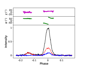
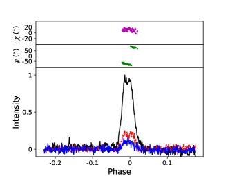
Figure 11: Integrated profiles of the first mode (Q, left) and the second mode (B’, right). Lines’ and dots’ meanings are same as Figure 1.

The flux of the two modes on 20230816 is also estimated in the same way of Section 3.1.3, and the result is shown in Figure 12. Both from the flux comparison and the waterfall plot, B’ mode’ intensity is much weaker than Q mode’s.

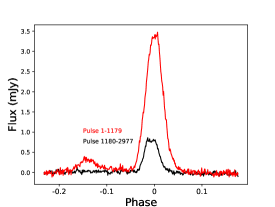
Figure 12: The comparison between B’ mode average profile’s (black line) and Q mode average profile’s (red line) flux under FAST L band, in 20230816 epoch.

3.2 Geometry and single pulses’ polarization

3.2.1 RVM fitting and the polar cap geometry

The total integrated profile (made by adding 4 epochs’ profiles together) is presented in Figure 13. Similarly integrated profiles of B mode and Q mode are given in Figure 14. The polarization position angle (PA) curves can be well fitted using the Rotation Vector Model (RVM, Radhakrishnan & Cooke 1969) in the form of Equation 13 ($\zeta=\alpha+\beta$). All four epochs’ pulse profiles could be fitted with the same $\alpha$, $\beta$ with slightly different $\psi_{0}$s (Figure 1). $90^{\circ}$ displacement of PA is permitted in the fitting for orthogonal polarization modes (OPMs). The fitting result is that the incline angle $\alpha=46\pm 2(^{\circ})$ and the impact angle $\beta=15\pm 3(^{\circ})$. PAs of the main pulse and the precursor are fitted with two RVM curves displaced by $90^{\circ}$ respectively, indicating that the main pulse and the precursor are orthogonal in linear polarization.

$$\tan(\psi-\psi_{0})=\dfrac{\sin(\phi-\phi_{0})\sin\alpha}{\sin\zeta\cos\alpha-\cos\zeta\sin\alpha\cos(\phi-\phi_{0})}$$ (13)

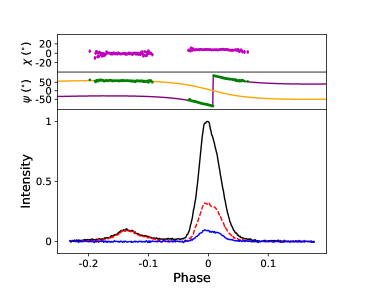
Figure 13: The integrated profile of all 4 observations. Lines’ and dots’ meanings are same as Figure 1.

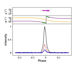
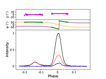
Figure 14: Integrated profiles of all the B modes (left, 3482 pulses) and the Q modes (right, 9235 pulses) in 4 observation epochs (by adding up signal-to-noise ratio). Lines’ and dots’ meanings are same as Figure 1.

Methods in Wang et al. (2023) and Qiao et al. (2004) are applied to map radiation to pulsar surface geometrically, with the help of two representative groups of magnetic field lines, and the result is shown in Figure 15. The core region lies inside feet of critical field lines, and the annular region lies between feet of critical field lines and last open field lines. B0943$+$10 has a small polar cap ($r<1^{\circ}$), and the spark discharge origin of precursor component radiation is generally further away from the magnetic axis than that of main pulse radiation.

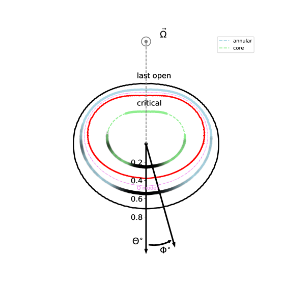
Figure 15: B0943$+$10’s radiation mapped to the surface polar cap region. The magnetic axis is right in the middle. Black solid line: feet of last open field lines (margin of the polar cap); red solid line: foots of critical filed lines (margin of the core gap region); light blue line: feet of typical magnetic field lines in annular gap region, having equal distances to last open field lines and critical field lines; green line: feet of typical magnetic field lines in core gap region, having $2/3$ distances of critical field lines to the magnetic axis. The dashed line’s part is invisible to our line of sight because of the radiating height exceeding the light cylinder; light purple dash-dotted line: feet of possible origin of Q mode radiation particles (will be discussed in Section 4.2 and 4.3), having equal distances to the light blue line and the solid red line; thick black lines with opacity: radiation mapped to those typical field lines’ feet. The opacity is positively correlated to the total intensity in the integrated profile shown in Figure 13.

Based on the mapping result, the radiation height (namely the distance from the tangential point of line-of-sight and magnetic field line of certain phase to the center of the pulsar) and radiation particles’ Lorentz factors ($\gamma$) (based on curvature radiation’s central frequency equation, see Equation 14) could also be estimated, and the results are shown in Figure 16. For B0943$+$10’s case, if the radiating particles originate from the annular region, they tend to radiate at a lower height with smaller Lorentz factor. And if both the main pulse component and the precursor component are radiated by particles from the annular region, the precursor component is emitted higher by particles with larger Lorentz factor. If both the main pulse component and the precursor component are radiated by particles from the core region, the particles radiating the precursor component still emits higher, but with slightly lower $\gamma$ comparing with that of the main pulse component’s peak.

$$f_{c}=\dfrac{1}{2\pi}\dfrac{3c\gamma^{3}}{2\rho_{c}}$$ (14)

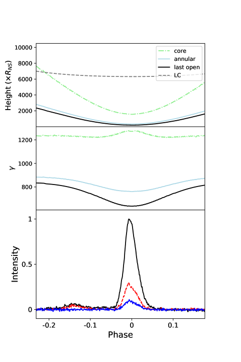
Figure 16: Upper panel: radiation height, the distance from the radiation position to the pulsar’s central point. Middle panel: Lorentz factors of radiation particles. Light green dotted dash line: heights and Lorentz factors calculated with the representative field lines in core region (the light green line in Figure 15); Light blue line: heights and Lorentz factors calculated with the representative field lines in annular region (the light blue line in Figure 15); Black line in upper panel: heights and Lorentz factors calculated with the last open field lines; Gray dashed line: distances from the pulsar’s central point to light cylinder in the radiating directions at certain phases. Lower panel: the profile in Figure 13.

3.2.2 Single pulses’ polarization distribution properties

B0943$+$10’s single pulses’ distributions of $L/I$, PA and ellipticity angle (EA) for all 4 epochs (14519 pulses in total) are shown in Figure 17’s left sub-figure. For the main pulse component phase range (-0.06, 0.06), there are PA patches located around $0^{\circ}$ and $\pm 90^{\circ}$, indicating the existence OPMs. OPMs can also be seen directly from some individual pulses’ PAs, like those shown in Figure 18. For the precursor component phase range (-0.2, -0.08), there is only one PA patch, which is on the same RVM curve with the main pulse PA patch around $0^{\circ}$. The respective dominating polarization modes of the main pulse and the precursor are orthogonal, which is in accord with the PA curve fitting results in Section 3.2.1. It is worth noticing that although the integrated profile shows circular polarization (Stokes $V$) of totally plus sign, a fraction of single pulses’ ellipticity angles are actually smaller than $0^{\circ}$, indicating some minus-sign $V$ appears in single pulses.

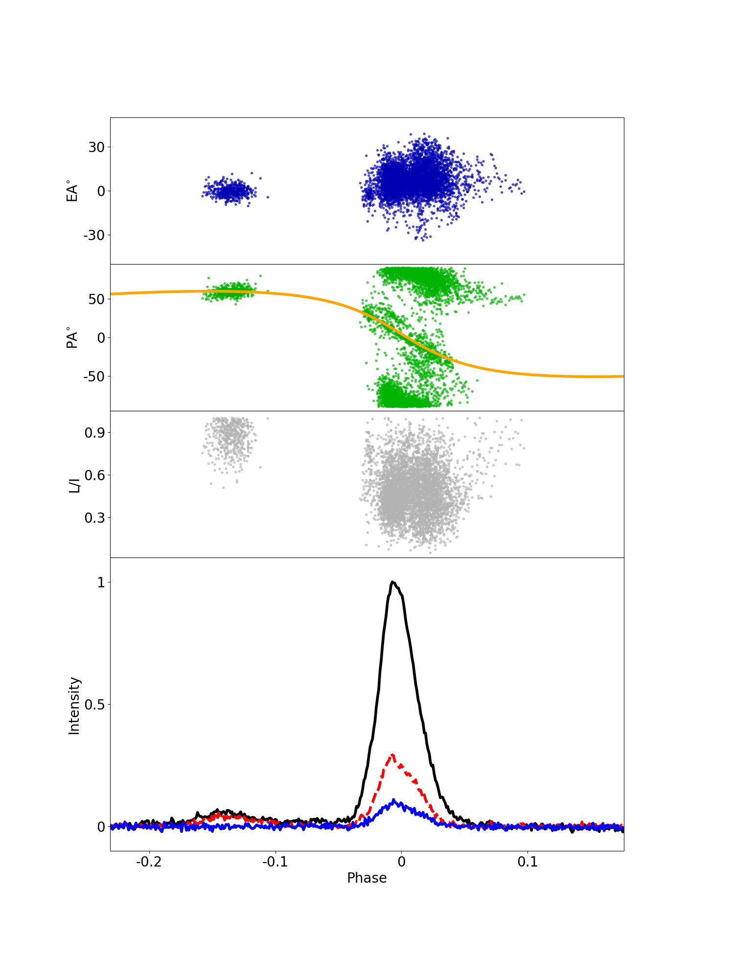
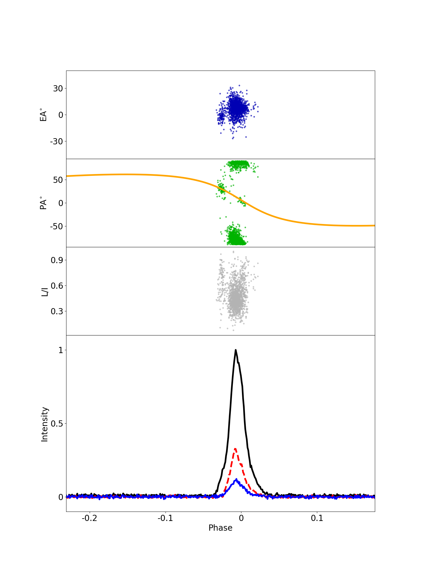
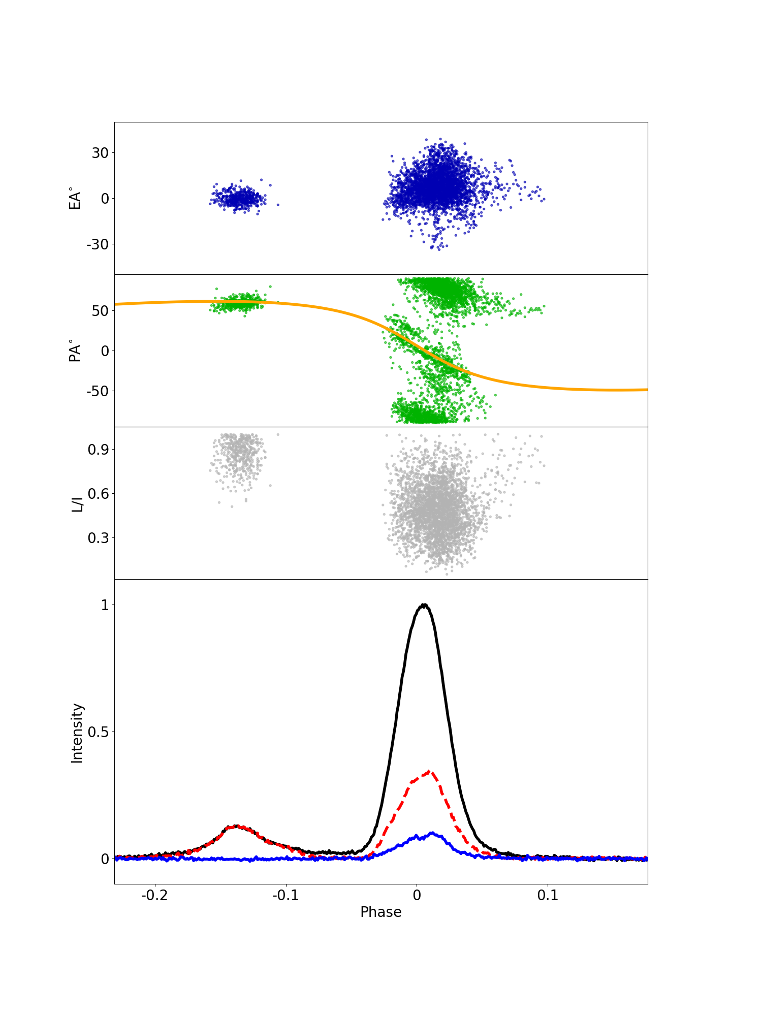
Figure 17: Distributions of PA, EA and $L/I$ of all 4 observation epochs’ 14519 pulses (left), all 3486 B mode pulses (middle) and all 9235 Q mode pulses (right). Panel 1 (1-4 from up to bottom): the integrated profiles of all pulses taken into account, where lines’ meanings are same as Figure 1; Panel 2: the distributions of $L/I$; Panel 3: the distributions of PA. Panel 4: the distributions of EA. Definitions of PA and EA follow Figure 1. Only single pulses’ bins where both $\sigma_{\text{PA}}\leq 5^{\circ}$ and $\sigma_{\text{EA}}\leq 5^{\circ}$ are included.

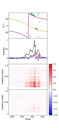
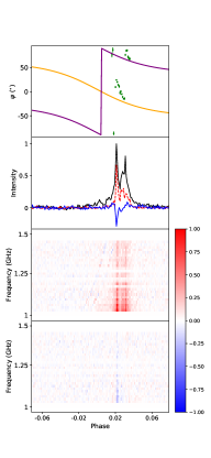
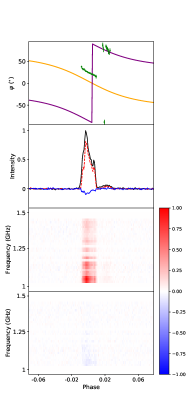
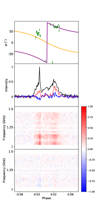
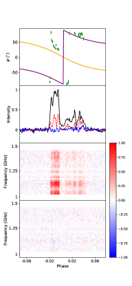
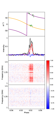
Figure 18: Examples of single pulses exhibiting orthogonal polarization modes. Panel 1 (1-4 from up to bottom): PA and RVM curves, where lines’ and dots’ meanings are same as Figure 1; Panel 2: individual pulse profiles of $I$, $L$ and $V$; Panel 3: dynamic spectrum of total intensity $I(\phi,\nu)$, where the 4096 frequency channels are binned into 32 bins. The intensity values are normalized with the maximum of $I(\phi,\nu)$; Panel 4: dynamic spectrum of circular polarization intensity $V(\phi,\nu)$, where the 4096 frequency channels are binned into 32 bins. The intensity values are normalized with the maximum of $I(\phi,\nu)$.

We wonder if different signs of EA (i.e. the signs of Stokes $V$) correspond to different PA patches (or equivalently, different OPMs). Figure 19 shows the relation between EAs and cosPAs with the points from Figure 17. From Figure 19 we find that pulse bins with PA around $\pm 90^{\circ}$ , which means a small value of cosPA, tend to have EA $>0$ ($V>0$). But for pulse bins with PA around $0^{\circ}$ , whose cosPAs are large ($0.8-1$), they are more likely to have EA $<0$ ($V<0$). Compared with the results of Deshpande & Rankin (2001), PA patch around $\pm 90^{\circ}$ is the primary polarization mode (PPM), and the PA patch around $0^{\circ}$ is the secondary polarization mode (SPM). The main pulse component has certain amounts of both PPM and SPM, but dominated by PPM. The precursor’s PAs are on the same RVM curve with SPM patch of the main pulse component, indicating that the precursor component is pure SPM.

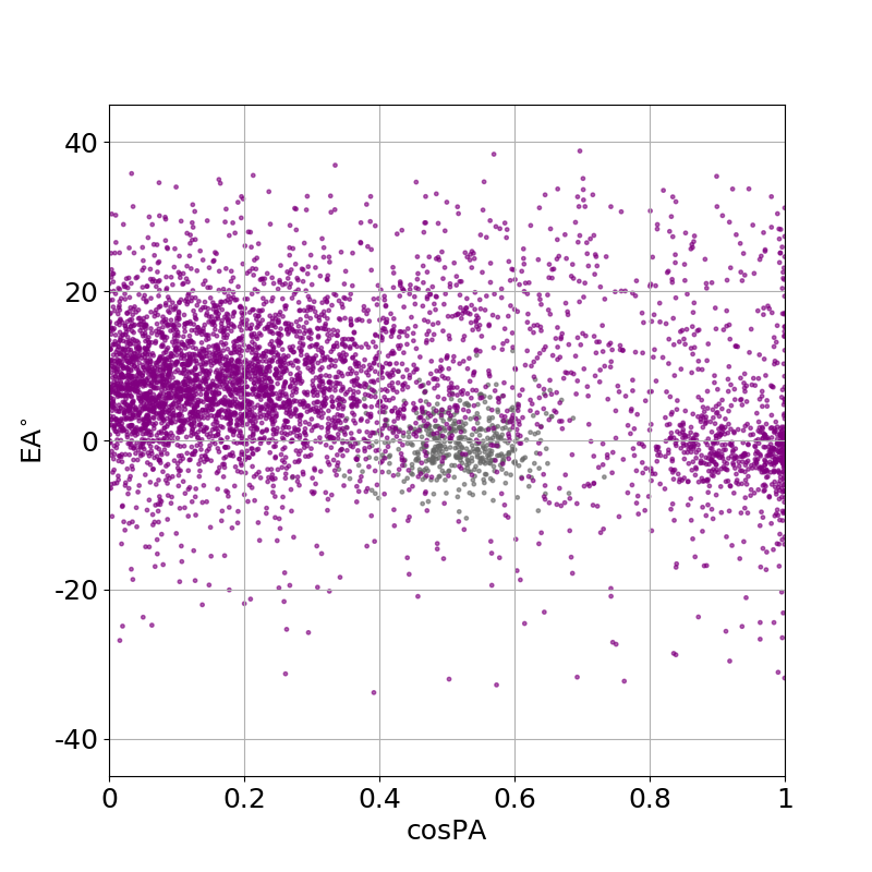
Figure 19: cosPA - EA distribution. Horizontal axis: cosPA; vertical axis: EA. Only single pulses’ bins where both the uncertainties $\sigma_{\text{PA}}\leq 5^{\circ}$ and $\sigma_{\text{EA}}\leq 5^{\circ}$ are included. Points from the precursor component is colored grey, while points from the main pulse component is colored purple.

The PA, EA and L/I distributions for B mode and Q mode are also shown in Figure 17, in the middle and right sub-figures. In Figure 17 for the B mode’s case (middle sub-figure), the extra component at phase $\phi\approx-0.025$ described in LRFSs in Section 3.1.2 and 3.1.3 also clearly appears. The extra component tends to have pure SPM PA patch, higher $L/I$ and more negative circular polarization than the main part of B mode pulse component.

In Figure 14, the maximum linear polarization proportion, which could be affected by orthogonal polarization modes, doesn’t vary evidently in main pulse components of B mode’s and Q mode’s integrated profiles. In order to figure out PPM and SPM’s proportion in B mode’s and Q mode’s main pulse component, we swing all PAs through RVM angles given by the orange curve in Figure 13, to make PPM and SPM more concentrated around $\pm 90^{\circ}$ and $0^{\circ}$. The process is equivalent to calculating PA with respect to the orange RVM curve. For example, if an individual pulse’s PA curve prefectly follows the RVM curve, then after swinging, its PA curve becomes a horizontal line at $0^{\circ}$. Marking Stokes $Q$ and $U$ at single phase bin $\phi$ as $Q(\phi)$ and $U(\phi)$, and the orange RVM curve value at $\phi$ as $\delta(\phi)$, practically the swing process could be denoted as:

$$\left(\begin{matrix}Q^{\prime}(\phi)\\ U^{\prime}(\phi)\\ \end{matrix}\right)=\left(\begin{matrix}\cos(2\delta(\phi))&\sin(2\delta(\phi))\\ -\sin(2\delta(\phi))&\cos(2\delta(\phi))\\ \end{matrix}\right)\left(\begin{matrix}Q(\phi)\\ U(\phi)\\ \end{matrix}\right)$$ (15)

After swinging, the PAs versus signal-to-noise ratios of intensity are shown in Figure 20. Regarding rotated PA points within range $(-45^{\circ},+45^{\circ})$ as SPM PA points, others as PPM PA points, PPM and SPM pulse bins’ numbers in B mode’s and Q mode’s main pulse component phase range are counted and shown in Table 2. If only considering highly polarized pulse bins sifted in Figure 17, 19 and 20, The proportion of SPM is larger in Q mode than in B mode.

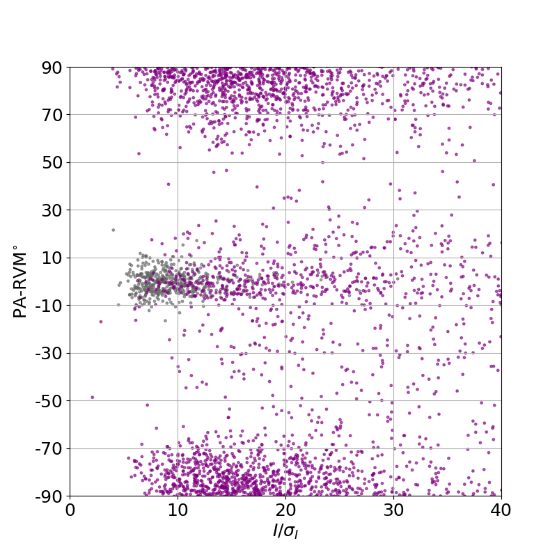
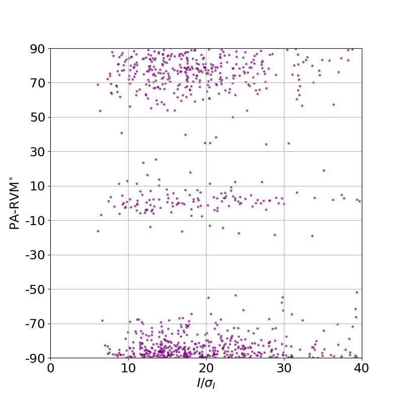
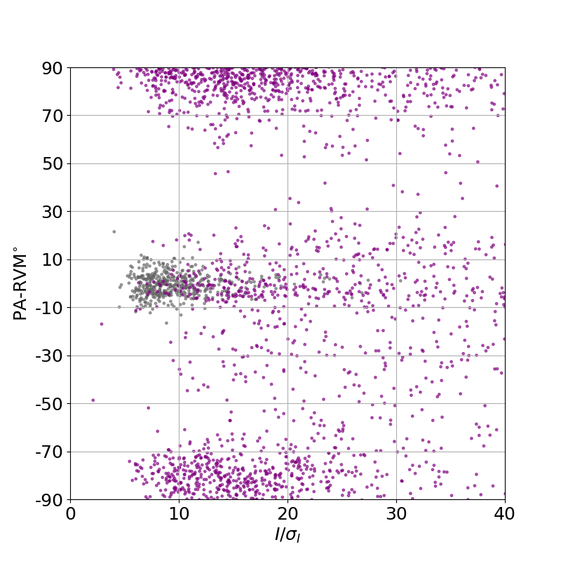
Figure 20: rotated PA - I distribution for total 14519 pulses in 4 epochs (left), all 3486 B mode pulses (middle), and all 9235 Q mode pulses (right). Horizontal axes: PA swinged through orange RVM curve in Figure 13; vertical axes: signal-to-noise ratios of intensity on pulse bins. Only single pulses’ bins where both the uncertainties $\sigma_{\text{PA}}\leq 5^{\circ}$ and $\sigma_{\text{EA}}\leq 5^{\circ}$ are included. Points from the precursor component is colored grey, while points from the main pulse component is colored purple.

Table 2: MAIN PULSE ORTHOGONAL MODES COUNTING

Radiation modes	Number of PPM	Number of SPM
	HIGHLY POLARIZED PULSE BINS
B mode	1311	146
Q mode	2520	1227
	FULL INDIVIDUAL PULSES
B mode	2522	964
Q mode	8318	917

However, a large part of weak pulses are ignored if we only consider highly polarized pulse bins. Weak pulses’ properties also significantly affect the integrated profiles’ linear polarization fraction. In order to take weak pulses into account, we swing their PAs through the orange RVM curve in Figure 13, and then add them together to calculate representative PA^∗s:

$$\text{PA}^{*}=0.5\arctan(\dfrac{\Sigma_{\phi}U^{\prime}(\phi)}{\Sigma_{\phi}Q^{\prime}(\phi)})$$ (16)

Although it has been mentioned above that both OPMs also appear in individual pulses (Figure 18), the PA^∗ could reveal the dominating orthogonal mode in an individual pulse. The relation between PA^∗s and total intensity signal-to-noise ratios of individual pulses are shown in Figure 21. Regarding pulses whose PA^∗s within range $(-45^{\circ},+45^{\circ})$ as SPM dominated pulses, others as PPM dominated pulses, the counting results are also shown in Table 2. The results show that B mode pulses are more dominated by SPM than Q mode. There tends to be more highly polarized pulses in PPM-dominated pulses (as is shown in Figure 17), so the mixture of SPM and PPM doesn’t bring significant differences bewteen B mode and Q mode in linear polarization decreasing

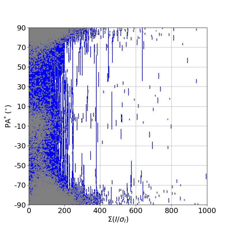
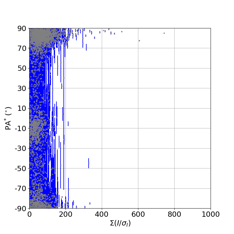
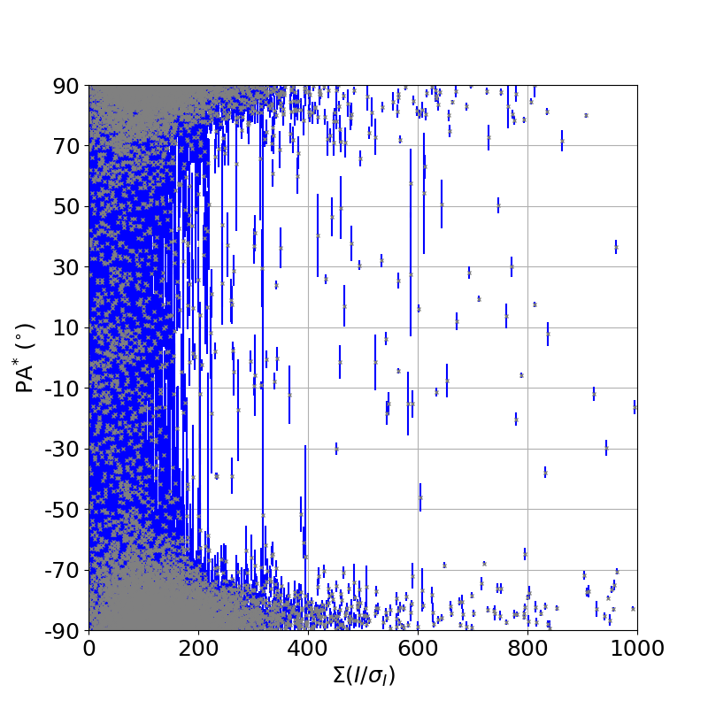
Figure 21: Total intensity signal-to-noise ratio - PA^∗ distributions of all 4 epochs’ 14519 pulses (left), all 3486 B mode pulses (middle) and all 9235 Q mode pulses (right). Horizontal axis: Total intensity signal-to-noise ratio; vertical axis: PA^∗ (with error bars). Each point represent one individual pulse.

4 Discussion

4.1 The profile evolution

The eigen modes shown in Figure 4 and Figure 9 have some phase bins with minus-sign $I$ or $L$. The negative values of $I$ and $L$ are not physical, but a way to reflect some certain changes in profile evolution, like those described in Section 3.1. Some evolution properties found with the eigen mode search algorithm are consistent with published results on B0943$+$10’s profile evolution. For example, the relation between the precursor’s and main pulse’s $I$ sign revealed by Eigen mode 3 is consistent with the result in Backus et al. (2010) (when the precursor component gets stronger, the main pulse component tends to be suppressed). But there are more newly discovered characteristics, like the strange-attractor-like weights’ evolution (Figure 5) and the quasi-periodicity of Eigen mode 4. The possible existence of strange attractor pattern in pulsar mode switches indicates that the pulsar dynamic system can be in chaos, switching between two or more states.

The B’ mode, though happens after a mode switch from Q mode, is different from the transitive modes reported in Suleymanova & Bilous (2023), because the B’ mode lasts for long ($>1000$ pulses). Suleymanova & Rodin (2014) reports a continuous increase in B mode’s flux, lasting several hours, after Q-to-B mode switch. So B’ mode may be a beginning status of B mode.

The extra component at phase $\phi\approx-0.025$ may be correspond to one of the components shown in the two-hump profiles under lower frequency bands (e.g., Deshpande & Rankin, 2001; Rankin et al., 2003). It may originate from a different height or position with the main part of B mode pulses, which makes it different in polarization and modulation properties.

Last but not least, the standard deviations of single pulses’ Stokes parameters of all epochs’ 14519 pulses are shown in Figure 22. It’s noticing that 20230816 epoch’s standard deviations of Stokes parameters are almost 3 times larger than that of other three epochs. If such difference is caused by some external events affecting telescope receiver like thundering, then we’ve underestimated the flux of the Q mode and B’ mode in 20230816 epoch.

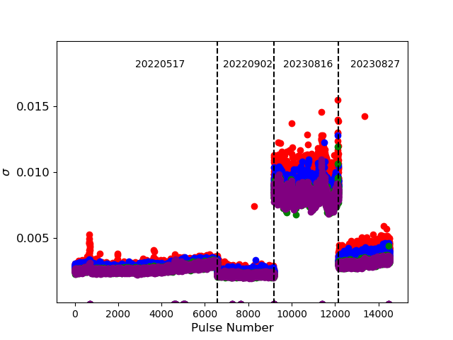
Figure 22: Standard deviations of single pulses’ Stokes parameters of all epochs’ 14519 pulses. Horizontal axis: pulse numbers; vertical axis: standard deviations of baseline values of the pulse profiles. Red: I; Purple: Q; Green: U; Blue: V.

4.2 The geometry and the polar cap region

A good RVM fitting indicates that at the particles radiating positions, the magnetic field is well described with a dipole field, which usually demands that the radiating position shouldn’t be too high from the pulsar surface. And the existence of sub-pulse drifting in the main pulse region suggests that radiation originate further from the magnetic axis, according to the carousel model in Ruderman & Sutherland (1975). We would then assume that that the source $e^{\pm}$-plasma is created just above pulsar surface with the field-lines whose foot-points are located inside the last open-field region. So from Figure 15 and  16, the polar cap’s annular region (region between feet of critical field lines and of last open field lines) might be a more reasonable birthplace of the radiating particles, for both the main pulse component and the precursor component. If we accept that statement, then comparing to the main pulse component, the precursor component is radiated higher from larger $\gamma$ radiating particles.

The RVM fitting result of B0943$+$10’s FAST L band observations is different from the frequently mentioned radiation geometry in former studies, namely the geometry given by Deshpande & Rankin (2001). Deshpande & Rankin (2001) calculates the geometry through radiation cone models (based on Rankin (1993)) to fit for both polarization angles and pulse profiles, and their results are $\alpha\approx 12^{\circ}$ and $\beta\approx-5^{\circ}$.

The geometry yielded by FAST observations may be more in accord with the X-ray radiation properties of B0943$+$10. XMM-Newton observations of B0943$+$10 (e.g., Hermsen et al., 2013) show that thermal X-ray pulsation appears significantly in Q mode, which could comes from a local high-temperature spot on the pulsar surface, namely a hotpot. Hermsen et al. (2013) points out the possible contradiction between the observed X-ray pulsation and the radiation geometry given by Deshpande & Rankin (2001), because when the magnetic axis, the spin axis and the line of sight are almost aligned (with small $\alpha$ and $\beta$ angles), the hotspot in the polar cap region is more likely to appear unmodulately and thus X-ray pulsation will not happen. In our result’s case, the axes are not so close to each other, making the hotspot modulation more feasible.

However, there still exists a question why thermal X-ray pulsation is significant in Q mode, but almost ceases in B mode. X-ray usually has few interactions with magnetized plasma, so it is more possible that some changes on pulsar surface happen during mode switch leading to differences in hotspots in different radiation modes.

A possible answer to this question lays in the origin of the precursor component. As is shown in Section 3, Q mode pulse profile has a precursor component while B mode has not. As is mentioned above, compared with the main pulse component, the precursor component is radiated higher (further from pulsar surface) by radiating particles with larger Lorentz factor $\gamma$. A simple picture on radiating particles (e.g., Ruderman & Sutherland, 1975) is that all primary particles are accelerated to very large $\gamma_{\text{primary}}$ ($\sim 10^{6}$) near the pulsar surface, and then flow along magnetic field lines, losing energy through curvature radiation, and high-energy photons produce secondary particles. After several turns of cascade reactions, finally radiating particles radiate radio frequency waves at certain heights, which is observed by us. According to estimations of primary particles’ Lorentz factor like Sob’yanin (2023), We state that since the precursor component’s radiating particles have larger Lorentz factors and has gone through longer ways along magnetic field lines losing more energy, the precursor component may originate from primary particles with larger $\gamma_{\text{primary}}$ than those contribute to the main pulse component.

High-energy primary particles and secondary particles can flow back and hit the surface to form hotspots which lead to X-ray emission (e.g., Zhang & Harding, 2000; Harding & Muslimov, 2001). Under such logic, the component with higher-energy primary particles might be related with a hotter hotspot. In B0943$+$10’s case, the hotspot associated with the precursor component is hotter than the hotspot associated with the main pulse component. It’s also possible that the precursor component, or the Q mode profile as a whole, originates nearer to the magnetic axis than B mode (like the light purple dash-dotted line in Figure 15), which results in higher energy secondary particles for Q mode radio radiation origin. All two processes above make Q mode X-ray pulsation stronger than B mode.

The precursor component’s stimulation may be caused by some local changes on pulsar surface, like a “zit” appearing on the rough surface (Xu & Wang, 2023; Wang et al., 2023) that makes local electric field grow larger, leading to spark discharges. The birth of a new spark discharge point may suppress sparking near it (Beskin, 1982), which may explain the main pulse component intensity’s anticorrelation with the precursor component intensity pointed out in Section 4.1. The stimulation of the precursor component produces more charged particles into the magnetosphere, and probably leading to changes in radio waves’ propagation.

The results in Figure 16 also provide possible explanations to some other phenomena observed. (1) Since the precursor component is radiated relatively closer to the light cylinder than the main component, the precursor radiation undergoes less propagation effects, which could explain why the precursor component has high $L/I$ but almost no circular polarization. (2) At lower frequency bands, the curves in the “Height” panel of Figure 16 will have a overall shift to higher heights (according to radius-frequency-mapping). When the frequency is too low, the precursor component’s theoretical radiation height may exceed the light cylinder, which could cause the precursor component to actually be weaken, like Fig. 2 in Hermsen et al. (2013): comparing to the main pulse component, the precursor component is relatively much weaker under LOFAR 140MHz observation than under GMRT 320MHz observation.

We’d like to mention that in pulse profile plots with fitted RVM curves (Figure 1, 13 and 14), the phase locations of main pulses’ peaks are all close to phase $\phi=0$, namely the centroid of the RVM curve. If considering BCW shift described in Blaskiewicz et al. (1991), using the radiation height shown in Figure 16 (at $\phi=0$, height $r\approx 300R_{\text{NS}}\approx 3\times 10^{8}$cm), the BCW shift will be $\Delta\phi\approx 0.04$, which is apparently much larger than what we’ve observed. This may indicate that the birthplace of radiation particles are actually more close to the feet of last open field lines, which means that radiation heights are actually lower (see Figure 16 for the case of last open field lines) than we’ve estimated in Section 16. Besides, radio radiation’s propagating through polarization limiting region will also reduce the BCW shift (e.g., Barnard, 1986; Blaskiewicz et al., 1991). Anyway, if BCW shift does work, the intensity profile’s centroid will move to $\phi\approx-0.04$, which actually doesn’t affect our main conclusion that the precursor component is radiated higher by charged particles with higher energy.

4.3 The OPMs and propagation effects in magnetosphere

OPMs in pulsar are usually interpreted as O (ordinary) mode and X (extraordinary) mode for high frequency waves propagating in plasma. Theories (e.g., Petrova, 2001) suggest that while curvature radiating particles only emit O mode waves, OPMs are formed due to mode coupling and conversion in pulsar magnetosphere, and O-mode and X-mode could have different directions of circular polarization after propagating through polarization-limiting region. Such phenomena are observed on B0943$+$10 (Figure 19) and also on other pulsars like PSR B2020$+$28 (Cordes et al., 1978). We wonder if it’s common or uncommon. Besides, from individual pulses shown in Figure 18 both orthogonal modes could be observed in one single pulse, and this may also support OPM’s originating from propagation.

If adapting criterion given by Andrianov & Beskin (2010) and Beskin & Philippov (2012), where O-mode has minus sign of $(d\text{PA}/d\phi)\cdot V$ and X-mode has plus sign of $(d\text{PA}/d\phi)\cdot V$, then for the main pulse component, PA patches around $\pm 90^{\circ}$ (PPM) corresponds to O-mode, while PA patches around $0^{\circ}$ (SPM) corresponds to X-mode, and the precursor component consists of only X-mode. Under this framework, Section 3.2.2 also shows that B mode and Q mode pulses have different proportions of O-mode and X-mode. O-mode and X-mode have different ways of propagating in magnetosphere (e.g., Barnard & Arons, 1986; Petrova & Lyubarskii, 2000; Andrianov & Beskin, 2010), so the difference in OPMs’ proportion for B and Q modes may be caused by a global change in magnetosphere (models like Timokhin (2010)). The spin down rate may also be affected. It’s possible to give a picture of B-to-Q mode switch that something happening on the pulsar surface gives rise to quick changes of sparking regions in the polar cap and of some physical parameters (like the particle number density (e.g., Kramer et al., 2006)) of magnetosphere, leading to both the precursor component’s appearance and some O-mode waves changing into X-mode. However, it’s hard to understand why the precursor component is pure X mode, if we accept that it is radiated much higher than the main pulse component and propagates less distance in magnetosphere, as is stated in Figure 16.

If we make the opposite statement, that for the main pulse component, PA patches around $\pm 90^{\circ}$ (PPM) corresponds to X-mode, while PA patches around $0^{\circ}$ (SPM) corresponds to O-mode, and the precursor component consists of only O-mode, it’s natural for the precursor component’s being radiated higher and being less affected by propagation effect. Under this statement, the O-mode is largely converted or absorbed for both B mode and Q mode pulses. Q mode pulses have more highly polarized O-mode “survived”, so maybe magnetosphere plasma number density is lower in Q mode’s case. Another possible mechanism is that when the pulsar switches from B mode to Q mode, the region closer to the magnetic axis (like the light purple line in Figure 15) begins to spark due to some changes on the pulsar surface, giving birth to some radiating particles. They may radiate at higher altitude, whose strong radiation are slightly less likely to be X mode because of less propagation in magnetosphere. Anyway, those physical processes may need more detailed investigations.

Last but not least, it has been reported that planets are found around B0943$+$10 (Suleymanova & Rodin, 2014; Starovoit & Suleymanova, 2019). Suleymanova & Rodin (2014) suggests that B0943$+$10’s mode switch and X-ray emission are caused by surrounding matter’s accretion. The accretion could lead to changes in magnetosphere and hotspots’ formation on pulsar surface, too. To judge whether mode switch is triggered by surface change or external accretion, more observations on other wavelengths are needed.

5 Conclusion

PSR B0943$+$10 is observed by FAST at 1-1.5GHz. The radiation modes in all 4 observation epochs are analyzed. The mode switch process could be quantitatively described with the results of an eigen mode searching algorithm. The mixture weights of the two most significant eigen modes appear jumps that representing the mode switch process, and a strange-attractor-like pattern in 2D plane, suggesting the pulsar system switches between certain states. Under FAST L band, Q mode is almost as bright as B mode, indicating different frequency evolution between modes. An extra component is found in B mode pulses around phase $\phi\approx-0.025$.

Rotating vector model fitting of the integrated profile’s polarization angles gives a geometry of $\alpha=46^{\circ}$ and $\beta=15^{\circ}$. The precursor component and the main pulse component are orthogonally polarized. Based on this geometry we map the radiation to some representative magnetic field lines starting from the polar cap on the pulsar surface and estimate the radiation height and radiation particles’ Lorentz factors. We conclude that B0943$+$10’s L band radiation particles are more likely to originate from the annular region of the polar cap than the core region. Comparing to the main pulse component radiation, B0943$+$10’s precursor component radiation comes from a further place from the magnetic axis, has higher radiation height and larger Lorentz factors of radiation particles. So the precursor component may have initial particles with higher energy, leading to a hotter hotspot on pulsar surface. The precursor component only appears in Q mode, so B0943$+$10 may have considerable thermal X ray pulsation only in Q mode, which is consistent with former X-ray observations. The precursor component’s stimulation may be related to the trigger of mode switch.

On the other hand, single pulses’ polarization properties are studied. B0943$+$10’s different orthogonal polarization modes (OPMs) tend to have different directions of circular polarization, which could be used to relate observed OPMs to ordinary and extraordinary wave modes in plasma. The proportion of OPMs changes with mode switches. Some individual pulses also appear with both two orthogonal modes. The results may support OPMs’ origin from wave propagation in magnetosphere, and could indicate that magnetosphere’s parameters change during mode switch processes.

Appendix A Waterfall plots for 20220517 and 20230827 epochs

Figure 23 and 24 show waterfall plots of 6567 pulses in 20220517 epoch, which are pure Q mode. Figure 25 shows the waterfall plots of 2358 pulses of 20230827 epoch, which are pure B mode.

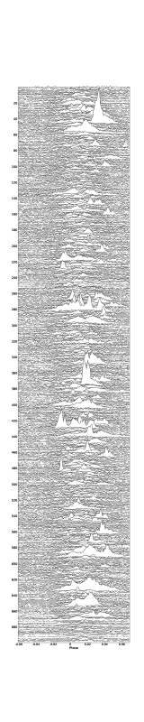
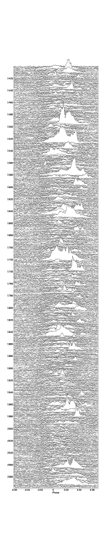
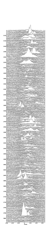
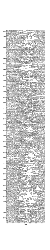
Figure 23: Waterfall plot of 6567 pulses in 20220517 observation (part 1). Horizontal axis: phase (0-1 for a period); vertical axis: number of pulses ($N$, top to bottom).

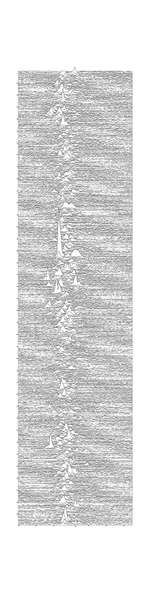
Figure 25: Waterfall plot of 2359 pulses in 20230827 observation. Horizontal axis: phase (0-1 for a period); vertical axis: number of pulses ($N$, top to bottom).

Appendix B Longitude Resolved Fluctuation Spectral (LRFS)

In all LRFSs shown below, a peak of 0.023 cycle/P appears in FFT spectral. Because the fluctuation is not only in on-pulse phase range but also in off-pulse phase range, this peak is not physical related to pulsar itself, but more likely to be caused by data processing.

References

- Andrianov & Beskin (2010) Andrianov, A. S., & Beskin, V. S. 2010, Astronomy Letters, 36, 248
- Backus et al. (2010) Backus, I., Mitra, D., & Rankin, J. M. 2010, MNRAS, 404, 30
- Backus et al. (2011) —. 2011, MNRAS, 418, 1736
- Barnard (1986) Barnard, J. J. 1986, ApJ, 303, 280
- Barnard & Arons (1986) Barnard, J. J., & Arons, J. 1986, ApJ, 302, 138
- Beskin (1982) Beskin, V. S. 1982, Soviet Ast., 26, 443
- Beskin & Philippov (2012) Beskin, V. S., & Philippov, A. A. 2012, MNRAS, 425, 814
- Bilous et al. (2014) Bilous, A. V., Hessels, J. W. T., Kondratiev, V. I., et al. 2014, A&A, 572, A52
- Blaskiewicz et al. (1991) Blaskiewicz, M., Cordes, J. M., & Wasserman, I. 1991, ApJ, 370, 643
- Cordes et al. (1978) Cordes, J. M., Rankin, J., & Backer, D. C. 1978, ApJ, 223, 961
- Deshpande & Rankin (1999) Deshpande, A. A., & Rankin, J. M. 1999, ApJ, 524, 1008
- Deshpande & Rankin (2001) —. 2001, MNRAS, 322, 438
- Hao et al. (2023) Hao, L., Li, Z., Huang, Y., et al. 2023, MNRAS, submitted
- Harding & Muslimov (2001) Harding, A. K., & Muslimov, A. G. 2001, ApJ, 556, 987
- Hermsen et al. (2013) Hermsen, W., Hessels, J. W. T., Kuiper, L., et al. 2013, Science, 339, 436
- Hobbs et al. (2006) Hobbs, G. B., Edwards, R. T., & Manchester, R. N. 2006, MNRAS, 369, 655
- Hotan et al. (2004) Hotan, A. W., van Straten, W., & Manchester, R. N. 2004, PASA, 21, 302
- Jiang et al. (2020) Jiang, P., Tang, N.-Y., Hou, L.-G., et al. 2020, Research in Astronomy and Astrophysics, 20, 064
- Kramer et al. (2006) Kramer, M., Lyne, A. G., O’Brien, J. T., Jordan, C. A., & Lorimer, D. R. 2006, Science, 312, 549
- Luo et al. (2020) Luo, R., Wang, B. J., Men, Y. P., et al. 2020, Nature, 586, 693
- Petrova (2001) Petrova, S. A. 2001, A&A, 378, 883
- Petrova & Lyubarskii (2000) Petrova, S. A., & Lyubarskii, Y. E. 2000, A&A, 355, 1168
- Qiao et al. (2004) Qiao, G. J., Lee, K. J., Wang, H. G., Xu, R. X., & Han, J. L. 2004, ApJ, 606, L49
- Radhakrishnan & Cooke (1969) Radhakrishnan, V., & Cooke, D. J. 1969, ApL, 3, 225
- Rankin (1993) Rankin, J. M. 1993, ApJ, 405, 285
- Rankin & Suleymanova (2006) Rankin, J. M., & Suleymanova, S. A. 2006, A&A, 453, 679
- Rankin et al. (2003) Rankin, J. M., Suleymanova, S. A., & Deshpande, A. A. 2003, MNRAS, 340, 1076
- Ruderman & Sutherland (1975) Ruderman, M. A., & Sutherland, P. G. 1975, ApJ, 196, 51
- Sob’yanin (2023) Sob’yanin, D. N. 2023, Phys. Rev. D, 107, L081301
- Starovoit & Suleymanova (2019) Starovoit, E. D., & Suleymanova, S. A. 2019, Astronomy Reports, 63, 310
- Suleymanova & Bilous (2023) Suleymanova, S. A., & Bilous, A. V. 2023, A&A, 675, A87
- Suleymanova et al. (1998) Suleymanova, S. A., Izvekova, V. A., Rankin, J. M., & Rathnasree, N. 1998, Journal of Astrophysics and Astronomy, 19, 1
- Suleymanova et al. (2021) Suleymanova, S. A., Kazantsev, A. N., Rankin, J. M., & Logvinenko, S. V. 2021, MNRAS, 502, 6094
- Suleymanova & Rankin (2009) Suleymanova, S. A., & Rankin, J. M. 2009, MNRAS, 396, 870
- Suleymanova & Rodin (2014) Suleymanova, S. A., & Rodin, A. E. 2014, Astronomy Reports, 58, 796
- Timokhin (2010) Timokhin, A. N. 2010, MNRAS, 408, L41
- van Straten & Bailes (2011) van Straten, W., & Bailes, M. 2011, PASA, 28, 1
- van Straten et al. (2010) van Straten, W., Manchester, R. N., Johnston, S., & Reynolds, J. E. 2010, PASA, 27, 104
- Vitkevich et al. (1969) Vitkevich, V. V., Alekseev, Y. I., Zhuravlev, V. F., & Shitov, Y. P. 1969, Nature, 224, 49
- Wang et al. (2023) Wang, Z., Lu, J., Jiang, J., et al. 2023, arXiv e-prints, arXiv:2308.07691
- Weisberg et al. (1999) Weisberg, J. M., Cordes, J. M., Lundgren, S. C., et al. 1999, ApJS, 121, 171
- Xu & Wang (2023) Xu, R., & Wang, W. 2023, Astron. Nachr., e20230153 (arXiv:2312.05510)
- Zhang & Harding (2000) Zhang, B., & Harding, A. K. 2000, ApJ, 532, 1150