Fluctuation-based Adaptive Structured Pruning for Large Language Models

Abstract

Network Pruning is a promising way to address the huge computing resource demands of the deployment and inference of Large Language Models (LLMs). Retraining-free is important for LLMs’ pruning methods. However, almost all of the existing retraining-free pruning approaches for LLMs focus on unstructured pruning, which requires specific hardware support for acceleration. In this paper, we propose a novel retraining-free structured pruning framework for LLMs, named FLAP (FLuctuation-based Adaptive Structured Pruning). It is hardware-friendly by effectively reducing storage and enhancing inference speed. For effective structured pruning of LLMs, we highlight three critical elements that demand the utmost attention: formulating structured importance metrics, adaptively searching the global compressed model, and implementing compensation mechanisms to mitigate performance loss. First, FLAP determines whether the output feature map is easily recoverable when a column of weight is removed, based on the fluctuation pruning metric. Then it standardizes the importance scores to adaptively determine the global compressed model structure. At last, FLAP adds additional bias terms to recover the output feature maps using the baseline values. We thoroughly evaluate our approach on a variety of language benchmarks. Without any retraining, our method significantly outperforms the state-of-the-art methods, including LLM-Pruner and the extension of Wanda in structured pruning. The code is released at https://github.com/CASIA-IVA-Lab/FLAP.

Introduction

Large Language Models (LLMs) (Brown et al. 2020; Touvron et al. 2023; Zhang et al. 2022; Scao et al. 2022) have recently achieved outstanding performance across various language benchmarks in NLP (Bommarito and Katz 2022; Bubeck et al. 2023; Wei et al. 2022), spurring a large number of open-source applications (Taori et al. 2023; Anand et al. 2023; Richards 2023). These remarkable capabilities typically come with a huge-scale model size with high inference costs. This makes it harder for more people to benefit from LLMs. Due to the computational resource constraints, most of the model compression methods in the pre-LLM era are no longer feasible for LLMs. Model compression methods for LLMs to date focus on model quantization (Dettmers et al. 2022; Xiao et al. 2023; Frantar et al. 2023; Dettmers et al. 2023) and unstructured pruning (Sun et al. 2023; Frantar and Alistarh 2023).

Structured pruning (He and Xiao 2023), which prunes entire rows or columns of weights, offers a promising solution to the deployment challenges of LLMs. Unlike unstructured pruning, structured pruning reduces both parameters and inference time without relying on specific hardware, making it more widely applicable (Anwar, Hwang, and Sung 2017). For effective structured pruning, it’s crucial to have a metric that captures the collective significance of an entire row or column. However, current unstructured pruning techniques for LLMs, as seen in methods like (Sun et al. 2023; Frantar and Alistarh 2023), primarily focus on the importance of individual elements of each row in isolation. This absence of structured metrics that evaluate entire rows or columns makes them less suitable for structured pruning. The recent LLM-Pruner (Ma, Fang, and Wang 2023) attempted structured pruning for LLMs, but its dependence on LoRA fine-tuning (Hu et al. 2021) creates a tough trade-off between high computation and effective pruning, limiting its use in larger models.

Pruning essentially involves two key aspects: discovering redundancy and recovering performance. For an effective structured pruning method tailored to LLMs, three fundamental criteria must be satisfied: a) a structured importance metric to discover structured redundancy; b) a mechanism for adaptively searching the optimal global compression model structure; and c) a compensation strategy to minimize performance degradation.

In response to these three essential criteria, we introduce FLAP (FLuctuation-based Adaptive Structured Pruning), a novel structured pruning framework. We find that certain channels of hidden state features exhibit structured sample stability. This observation enables us to compensate for bias within the model using baseline values. Specifically, we design a structured pruning metric that estimates the fluctuation of each input feature relative to the baseline value, utilizing a set of calibration samples. This metric assists in determining whether the output feature map can be recovered when a column of the weight matrix is removed. We then standardize these fluctuation metric scores across layers and modules separately, allowing for the adaptive determination of the global compressed model structure. Finally, FLAP employs the baseline values to add additional biases, recovering the output feature maps for the corresponding layers. Remarkably, our method avoids the need for the retraining process and requires only a single forward pass for both pruning and bias compensation, thereby maintaining low memory overhead.

We evaluate the effectiveness of FLAP on the LLaMA model family, and FLAP achieves remarkable performance on a variety of language benchmarks. Impressively, without any retraining, our method significantly outperforms the state-of-the-art methods, including LLM-Pruner and the extension of Wanda in structured pruning.

Our main contributions are listed as follows:

• We propose a novel retraining-free structured pruning framework for LLMs named FLAP. To our best knowledge, this is the first work that identifies the characteristic of structured sample stability in LLMs.

• The proposed framework uses a bias compensation mechanism, a pruning performance recovery method that does not require retraining. This mechanism yields greater benefits, especially under large pruning ratios.

• Our method achieves remarkable performance on a variety of language benchmarks and outperforms the state-of-the-art method without any retraining.

Related Works

Network Pruning Methods

Network pruning is a model compression technique that identifies and eliminates redundancy in the structure or parameters of a neural network, based on specific pruning metrics, and incorporates methods to recover model performance (LeCun, Denker, and Solla 1989; Hassibi, Stork, and Wolff 1993; Han et al. 2015). Pruning methods fall into two categories: unstructured pruning and structured pruning. Unstructured pruning is performed at the individual weight level, allowing for a large sparsity but failing to achieve real inference acceleration or storage reduction (Zafrir et al. 2021; Han, Mao, and Dally 2016). Within unstructured pruning, there exists a specialized variant known as semi-structured pruning. This approach enforces exactly N non-zero values in each block of M consecutive weights (Zhou et al. 2021). This approach has gained traction recently, particularly with support on newer NVIDIA hardware (Mishra et al. 2021). Structured pruning, by contrast, operates on entire rows or columns of weights, providing a more hardware-friendly solution that reduces storage requirements and enhances inference speed (Xia, Zhong, and Chen 2022; Molchanov et al. 2017).

However, conventional structured pruning methods typically rely on retraining (sometimes iteratively) to regain the performance of the pruned model (Han et al. 2015; Tan and Motani 2020; Han, Mao, and Dally 2016). Such methods pose scalability challenges for billion-scale LLMs due to constraints on memory and computational resources. Therefore a retraining-free structured pruning method for LLMs is very critical.

Large Language Model Compression

Large Language Models usually consist of billions of parameters, and their gradient backpropagation and training stage require large amounts of memory and computational resources. Consequently, many conventional model compression techniques have become infeasible for LLMs (Frantar and Alistarh 2023). For instance, knowledge distillation (Hinton, Vinyals, and Dean 2015), once a practical approach, now faces implementation challenges due to high training costs. Existing compression methods for LLMs mainly include post-training quantization (Dettmers et al. 2022; Xiao et al. 2023; Frantar et al. 2023; Dettmers et al. 2023) and post-training pruning (Sun et al. 2023; Frantar and Alistarh 2023). Our method also falls into the category of post-training pruning. It utilizes bias compensation to recover model performance, effectively avoiding the high computational cost of retraining. Unlike the past post-training pruning methods, our method is designed for the features of structured pruning of LLMs.

Properties of LLMs

Our work is related to the distinct properties of Large Language Models (LLMs) that have inspired various model compression techniques (Sun et al. 2023; Dettmers et al. 2023, 2022). Dettmers et al. (Dettmers et al. 2022) observed the emergence of channels with abnormally large magnitudes in the hidden state features of LLMs once they exceed a certain parameter scale (e.g., 6B). They suggest that this is the reason why existing quantization methods fail on LLMs. In response, they introduced a novel mixed-precision quantization technique. Contrary to the focus of previous work on the outlier magnitudes in LLMs, our research pivots towards investigating the structured stability within the channels of input features in these models. In our study, we find that certain channels within the hidden state features demonstrate consistent structured sample stability. This discovery offers invaluable insights for crafting structured post-training pruning algorithms, laying the foundation for the method we present in this paper.

Figure 1: Framework of the proposed FLAP. ①Measure the fluctuation of each channel across different layers and modules using calibration data; ②Standardize these fluctuation measures for a unified search method; ③Implement adaptive pruning ratios for each layer and module, employing bias compensation to restore model performance.

Preliminaries

Layer-Wise Pruning

Given the computational constraints, globally solving the pruning problem for Large Language Models (LLMs) is challenging. Layer-wise pruning becomes a practical solution under these constraints. Following this notion, SparseGPT (Frantar and Alistarh 2023) demonstrated that the challenge of unstructured pruning for LLMs can be tackled by decomposing it into individual layer-wise subproblems. This principle can be seamlessly extended to structured pruning within LLMs. The quality of solutions to these layer-wise subproblems can be evaluated based on the $\ell_{2}$-error. Given an input $\mathbf{X}^{\ell}$ of shape $\left(N,C_{in},L\right)$ where $N$ and $L$ represent batch and sequence dimensions respectively, and a weight $\mathbf{W}^{\ell}$ of shape $\left(C_{out},C_{in}\right)$, the $\ell_{2}$-error for structured pruning can be defined as:

$$\text{argmin}_{\mathbf{M}^{\ell}\in\mathbb{R}^{C_{in}},\widehat{\mathbf{W}}^{\ell}}||\mathbf{W}^{\ell}\mathbf{X}^{\ell}-(\mathbf{M}^{\ell}\odot\widehat{\mathbf{W}}^{\ell})\mathbf{X}^{\ell}||_{2}^{2}$$ (1)

where $\mathbf{M}^{\ell}\in\mathbb{R}^{C_{in}}$ represents the mask vector corresponding to the input channels, this vector mirrors whether each input channel is pruned or not. For the self-attention modules, these input channels are pruned in groups typically with sizes like group$\_$size=128. The term $\widehat{\mathbf{W}}^{\ell}$ denotes the possibly updated weights for the pruned layer. The notation $||\cdot||_{2}^{2}$ represents the $\ell_{2}$-error.

Local Pruning Metric Challenges

Regarding Eq. (1), the existing methods can be broadly categorized into two primary approaches: low-damage and easy-recoverability. These correspond to the core principles of OBD (LeCun, Denker, and Solla 1989) and OBS (Hassibi, Stork, and Wolff 1993), respectively. To illustrate, Wanda (Sun et al. 2023) uses a localized low-damage pruning metric to minimize harm to each layer’s output features. In contrast, SparseGPT (Frantar and Alistarh 2023) employs an easy-recoverability metric, aiming to identify components that other weights can compensate for during pruning. These approaches are insightful but tend to focus on the importance of individual elements in the weight matrix, neglecting the broader structured context. Such an atomistic approach is misaligned with structured pruning’s requirements, which demand a more global perspective that captures the collective importance of entire rows or columns in the matrix.

Methodology

In this section, we introduce FLAP, our proposed approach to structured pruning for Large Language Models (LLMs). FLAP encompasses three key components: Baseline Bias Compensation, Structured Fluctuation Metric, and Adaptive Structure Search. The overview of our method is presented in Figure 1.

Baseline Bias Compensation

In the context of structured pruning, the output of the layers of the uncompressed model can be decomposed into:

$$\mathbf{W}^{\ell}\mathbf{X}^{\ell}=\underbrace{(\mathbf{M}^{\ell}\odot\mathbf{W}^{\ell})\mathbf{X}^{\ell}}_{\text{retained}}+\underbrace{((1-\mathbf{M}^{\ell})\odot\mathbf{W}^{\ell})\mathbf{X}^{\ell}}_{\text{removed}}$$ (2)

The objective of structured pruning is to minimize the impact introduced by $\Delta Y^{\ell}=((1-\mathbf{M}^{\ell})\odot\mathbf{W}^{\ell})\mathbf{X}^{\ell}$ in the overall output feature map, thereby reducing the reconstruction error for each layer. For structured pruning of LLMs, the constraints are stronger, so the latter components cannot be simply removed. Therefore, a compensatory mechanism is essential to recover the model’s performance while adhering to the pruning structure.

We add an additional bias term to compensate for the damage inflicted on the output feature maps by the removed components. This bias term is designed to mitigate the reconstruction error introduced by the pruning process, allowing the pruned model to maintain high performance. In particular, we construct the bias term based on the baseline value, $\overline{\mathbf{X}}^{\ell}_{:,j,:}$, which represents the average of the $j$-th channel for all samples in layer $l$. As detailed in the following section, our empirical findings validate the effectiveness and feasibility of this compensatory approach. Specifically, the formulation for the baseline value is as follows:

$$\overline{\mathbf{X}}^{\ell}_{:,j,:}=\frac{1}{NL}\sum_{n=1}^{N}\sum_{k=1}^{L}\mathbf{X}^{\ell}_{n,j,k}$$ (3)

Once the mask $\mathbf{M}^{\ell}$ is established, the baseline value for the pruned channel can be seamlessly translated into the bias term for the linear layer as follows:

$$\mathbf{B}^{\ell}_{0} =\mathbf{W}^{\ell}((1-\mathbf{M}^{\ell})\odot\overline{\mathbf{X}}^{\ell})$$ (4)

$$\mathbf{W}^{\ell}\mathbf{X}^{\ell} \approx(\mathbf{M}^{\ell}\odot\mathbf{W}^{\ell})\mathbf{X}^{\ell}+\mathbf{B}^{\ell}_{0}$$

where $\mathbf{B}_{0}$ represents the bias of linear layer, which has a shape of $(C_{out},)$, and $\overline{\mathbf{X}}^{\ell}$ is a one-dimensional vector with dimensions $(C_{in},)$.

Structured Fluctuation Metric

Motivated by the observations from Figure 2, we note that certain channels of the hidden state features exhibit a low variation across different samples. This low fluctuation indicates that if their corresponding input feature channels are pruned, the resulted change in the output feature map can be effectively counterbalanced by the baseline value.

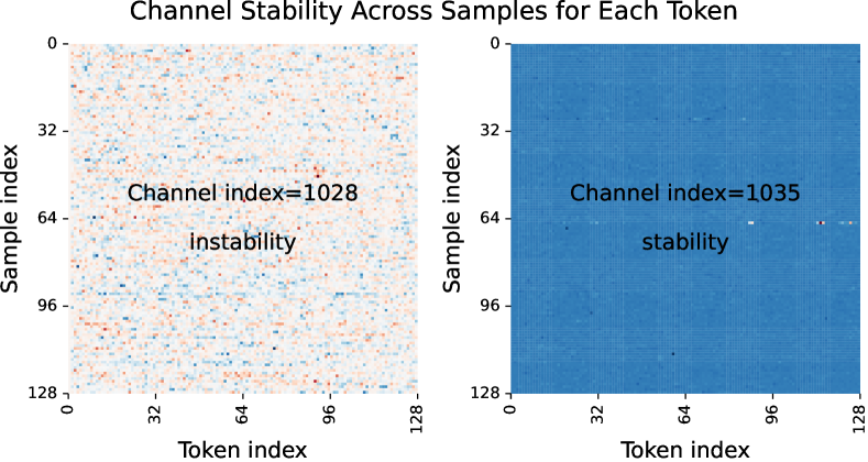
Figure 2: Certain channels of hidden state features exhibit structured sample stability. The left shows a channel with noticeable variations across samples, indicating low stability. The right displays a stable pattern common in many LLaMa channels.

As illustrated in Eq. (4), the structured easy-recoverability metric seeks to evaluate the impact on the output feature map when an input channel is substituted with its baseline value. A straightforward approach would involve individually substituting each input channel with its baseline value for the calibration samples and then computing the $\ell_{2}$-error between the output feature maps before and after this replacement.

However, such a method poses a significant computational challenge and is impractical for LLMs. To address this, we introduce an approximate metric for structured recoverability, which termed the ”fluctuation metric”. Specifically, we compute the sample variance of each input feature and weight it with the squared norm of the corresponding column of the weight matrix. Concretely, the score for the group of weight $\mathbf{W}^{\ell}_{:,j}$ is defined by:

$$\mathbf{S}^{\ell}_{:,j}=\frac{1}{N-1}\sum_{n=1}^{N}(\mathbf{X}^{\ell}_{n,j,:}-\overline{\mathbf{X}}^{\ell}_{:,j,:})^{2}\cdot||\mathbf{W}^{\ell}_{:,j}||^{2}_{2}$$ (5)

where $||\mathbf{W}^{\ell}_{:,j}||^{2}_{2}$ denotes the squared norm of $j$-th column of the weight matrix. $\frac{1}{N-1}\sum_{n=1}^{N}(\mathbf{X}^{\ell}_{n,j,:}-\overline{\mathbf{X}}^{\ell}_{:,j,:})^{2}$ represents the sample variance of the $j$-th channel of the input feature of layer $\ell$ under $N$ calibration samples. The denominator here is $\frac{1}{N-1}$. This correction is known as the Bessel correction and is used for unbiased estimation of the overall variance.

Adaptive Structure Search

The central challenge in layer-wise pruning revolves around adaptively searching the global compression model structures. Unifying different layers and modules without distinction can critically degrade performance. This issue arises because the magnitudes of the metrics across layers and modules vary greatly (Shi et al. 2023). Figure 3 demonstrates this by showing the mean values of the fluctuation metric for different modules in different layers.

Figure 3: Comparison of the average value of the fluctuation metric across different layers for different modules.

To ensure a consistent comparison of scores across different layers and modules, we standardize the metric distributions for each layer to a common mean and standard deviation. As defined in Eq. (5), the fluctuation metric captures the absolute variation in the output feature map when input features are replaced with their baseline values. In contrast, the standardized metric reflects the relative variation in the output feature map resulting from this replacement, making it suitable for a structured unified search. The standardized metric, denoted as, is formulated as follows:

$$\widehat{\mathbf{S}}^{\ell}_{:,j}=(\mathbf{S}^{\ell}_{:,j}-\mathbb{E}[\mathbf{S}^{\ell}_{:,j}])/(\mathbb{E}[[\mathbf{S}^{\ell}_{:,j}-\mathbb{E}[\mathbf{S}^{\ell}_{:,j}]]^{2}])^{\frac{1}{2}}$$ (6)

where $\mathbb{E}[\mathbf{S}^{\ell}_{:,j}]$ represents the expected value (or mean) of the vector $\mathbf{S}^{\ell}_{:,j}$. $(\mathbb{E}[[\mathbf{S}^{\ell}_{:,j}-\mathbb{E}[\mathbf{S}^{\ell}_{:,j}]]^{2}])^{\frac{1}{2}}$ represents the square root of the variance, which is the standard deviation.

Experiments

Experimental Settings

We conduct experiments on the LLaMA model family (LLaMA-7B/13B/30B/65B) to evaluate the efficacy of FLAP . Our evaluation focuses on language modeling performance on the WikiText2 (Merity et al. 2016) validation set and zero-shot performance across seven common sense benchmarks using the EleutherAI LM Harness (Gao et al. 2021). We compare FLAP against two previous pruning methods: Wanda-sp and LLM-Pruner. We generalize Wanda to structured pruning and name it as Wanda-sp. Detailed experimental settings, model descriptions, and evaluation protocols are provided in the Appendix A.

Method	Pruning Ratio	LLaMA
		7B	13B	30B	65B
Dense	0$\%$	12.62	10.81	9.11	8.21
Wanda-sp	20$\%$	22.12	16.83	11.66	11.76
LLM-Pruner		19.77	16.01	-	-
LLM-Pruner*		17.37	15.18	-	-
FLAP (Ours)		14.62	13.66	10.86	9.79
Wanda-sp	30$\%$	38.88	22.89	14.90	14.64
FLAP (Ours)		17.62	15.65	12.49	10.90
Wanda-sp	50$\%$	366.43	160.49	67.46	42.85
LLM-Pruner		112.44	-	-	-
LLM-Pruner*		38.12	-	-	-
FLAP (Ours)		31.80	24.20	19.36	15.30

Table 1: WikiText2 validation perplexity of pruning methods for LLaMA model family. * means with LoRA fine-tuning.

Language Modeling

Performance Comparisons.

For each of the LLaMA models, we present results at three distinct pruning ratios, as detailed in Table 1. Notably, FLAP significantly outperforms the other methods, achieving this superiority without any retraining. As the pruning ratio increases, the performance advantage of FLAP becomes more significant. To illustrate, consider the LLaMA-7B model: at a 50$\%$ pruning ratio, the LLM-Pruner exhibits a perplexity of 130.97, which improves to 39.02 after LoRA fine-tuning. In stark contrast, FLAP efficiently identifies sparse networks that yield a perplexity of 31.80, and remarkably, this is achieved without any retraining.

Remark.

The FLAP method, which requires no retraining, consistently outperforms the LLM-Pruner, even when the latter is fine-tuned with LoRA. Eq (4) offers insight into the potential reason for this superior performance. In FLAP , the baseline bias $\mathbf{B}_{0}$ is effectively treated as a low-rank component with a rank of $r=1$. Within the pruning framework of FLAP , bias compensation plays a pivotal role, serving a function similar to that of LoRA fine-tuning. This compensation helps to effectively recover the model’s performance after pruning.

Method	Pruning Ratio	BoolQ	PIQA	HellaSwag	WinoGrande	ARC-e	ARC-c	OBQA	Average
LLaMA-7B	0$\%$	73.18	78.35	72.99	67.01	67.45	41.38	42.40	63.25
Wanda-sp	20$\%$	71.25	77.09	72.77	67.09	71.09	42.58	41.60	63.35
LLM-Pruner		59.39	75.57	65.34	61.33	59.18	37.18	39.80	56.82
LLM-Pruner (w/ LoRA)		69.54	76.44	68.11	65.11	63.43	37.88	40.00	60.07
FLAP (Ours)		69.63	76.82	71.20	68.35	69.91	39.25	39.40	62.08
Wanda-sp	50$\%$	50.58	55.01	29.56	51.78	31.27	23.04	23.60	37.83
LLM-Pruner		52.57	60.45	35.86	49.01	32.83	25.51	34.80	41.58
LLM-Pruner (w/ LoRA)		61.47	68.82	47.56	55.09	46.46	28.24	35.20	48.98
FLAP (Ours)		60.21	67.52	52.14	57.54	49.66	29.95	35.60	50.37

Table 2: Zero-shot performance of the compressed LLaMA-7B. Bold results highlight the best performance. Underscored results denote the second-best performance for each pruning ratio.

Different Pruning Ratio.

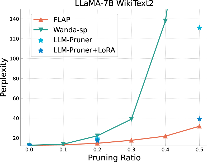
Figure 4: Results among FLAP and other structured pruning methods at varying pruning ratios on the LLaMA-7B WikiText2 dataset.

We evaluated the performance of each structured pruning method at various pruning ratios. As depicted in Figure 4, FLAP demonstrates remarkable stability in maintaining its performance as the pruning ratio increases. In contrast, Wanda-sp exhibits a sharp decrease in performance as the pruning ratio rises. Meanwhile, LLM-Pruner requires LoRA fine-tuning to maintain acceptable performance when the pruning ratio is increased to levels like 50$\%$.

Zero-shot Tasks Performance

We assessed the zero-shot capability of the pruned model across seven downstream tasks. As illustrated in Table 2, our method consistently outperforms LLM-Pruner with LoRA Fine-Tuning, achieving superior performance across varying pruning ratios, all without the need for retraining. At a 20$\%$ pruning ratio, Wanda-sp exhibits remarkable zero-shot capabilities, even surpassing the performance of the original, unpruned model. This suggests the presence of structured redundancy within LLMs that can be pruned away without necessitating retraining, thereby potentially enhancing model efficiency. However, when the pruning ratio is increased to 50$\%$, the performance of Wanda-sp suffers a significant degradation. In stark contrast, our method continues to excel, maintaining a clear advantage over other approaches. This finding demonstrates the efficacy of our structured pruning method in preserving the generalization capabilities of large language models (LLMs), even under stringent pruning conditions.

Ablation Study

We systematically examine three fundamental components of the FLAP method: the pruning metric, the global compression structure, and bias compensation. Additionally, we evaluate the robustness of our pruning approach in relation to calibration samples.

Pruning Metric.

Both the pruning metric and compressed model structure are critical factors in the pruning process. FLAP is specifically designed to address these two dimensions in the structured pruning of Large Language Models (LLMs). To evaluate their effectiveness, we conducted experiments employing various structured pruning metrics and global compression structures.

We investigated three structured pruning metrics in this study: 1) Weighted Input Feature Norm (WIFN), a low-damage metric assessing the effect of weight columns on the output feature map; 2) Input Feature Variance (IFV), used to gauge the variability among input features; and 3) Weighted Input Feature Variance (WIFV), utilized by FLAP to assist in determining the potential for recovery of the output feature map after a column of the weight matrix is removed.

To underscore the importance of global adaptive compression structure, we defined four configurations: ’UL-UM’ (Uniform across Layers and Modules, employed in unstructured pruning for LLMs like Wanda); ’UL-MM’ (Uniform across Layers, Manual ratio for Modules); ’AL-MM’ (Adaptive across Layers, Manual for Modules); and ’AL-AM’ (Adaptive across both Layers and Modules), the structure chosen by FLAP . Results in this section include bias compensation, with bias-compensated ablation experiments detailed later.

	Compressed model structure
Pruning Metric	UL-UM	UL-MM	AL-MM	AL-AM
WIFN: $\sum_{i=1}^{C_{out}}||\mathbf{X}^{\ell}_{j}||_{2}\cdot|\mathbf{W}^{\ell}_{ij}|$	84.79	128.75	34.50	34.09
IFV: $\frac{1}{N-1}\sum_{n=1}^{N}(\mathbf{X}^{\ell}_{n,j,:}-\overline{\mathbf{X}}^{\ell}_{:,j,:})^{2}$	55.41	48.87	35.72	33.33
WIFV: $\frac{1}{N-1}\sum_{n=1}^{N}(\mathbf{X}^{\ell}_{n,j,:}-\overline{\mathbf{X}}^{\ell}_{:,j,:})^{2}\cdot||\mathbf{W}^{\ell}_{:,j}||^{2}_{2}$	57.57	38.31	34.82	31.80

Table 3: Ablation on pruning metric and compressed model structure. Bold results denote the best compressed model structure found for each pruning metric. Underscored results indicate the best pruning metric found for each compressed model structure.

In our experiments, we structurally pruned the LLaMA-7B model with a 50$\%$ pruning ratio and evaluated the model using the perplexity metric on the WikiText2 dataset. The detailed results are presented in Table 3. Notably, the most effective pruning model was obtained using the default configuration of FLAP , achieving a perplexity of 31.80. The AL-AM global adaptive compression structure consistently outperformed other configurations under all evaluated pruning metrics, thereby effectively validating our proposed Adaptive Structure Search strategy. When analyzing the effectiveness of different global compression structures, we observed that various metrics present distinct strengths and weaknesses. Nevertheless, our proposed WIFV structured pruning metric displayed superior adaptability to the global compression structure.

Baseline Bias Compensation.

In structured pruning of large language models, restoring model performance after the pruning process is a crucial aspect. Our approach uniquely leverages bias compensation as a strategy to recover the performance of pruned models, circumventing the need for expensive and time-consuming retraining procedures. Figure 5 vividly illustrates the performance of the FLAP method on the WikiText2 dataset, comparing the perplexity scores with and without bias compensation at varying pruning ratios for the LLaMA-7B model. Evident from the figure, bias compensation plays a significant role in mitigating the performance degradation associated with pruning. Furthermore, this compensatory effect becomes more pronounced as the pruning ratio increases, highlighting the growing importance of bias compensation in more aggressively pruned models.

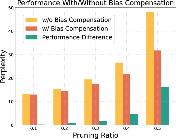
Figure 5: Performance comparison of the model with and without Bias Compensation at various pruning ratios. The yellow and orange bars represent the Perplexity of the model without and with Bias Compensation, respectively. The green bars show the performance difference between the two conditions.

Robustness to Calibration Samples.

Our method utilizes a calibration dataset to estimate the input variance at each layer of the language model. This makes it critical to investigate the impact of the size of this calibration dataset on the pruning performance. Figure 6 delineates the effects of varying the number of calibration samples on the pruning outcome. For this analysis, we set a pruning ratio of 50$\%$ for the LLaMa-7B model and observed the resultant perplexity on the WikiText2 dataset. The results clearly show that FLAP ’s performance improves as the size of the calibration dataset increases. In our experiments, we selected a default setting of 1024 calibration samples. Given that only a single forward propagation is required for this calculation, the computational cost associated with this sample size is minimal. Notably, the entire pruning process for the LLaMa-7B model is efficiently completed in a span of 3 to 5 minutes on a single GPU.

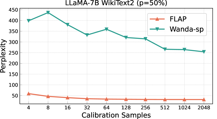
Figure 6: Robustness to Calibration Samples.

Inference Speed

Unlike unstructured pruning, structured pruning offers the dual benefit of reducing both the number of parameters and the inference time, without the need for specialized hardware. This makes structured pruning a more universally applicable approach. In this section, we empirically compare the actual parameter counts and inference speeds of different pruning methods, with the experiments conducted on NVIDIA A100 GPUs. The detailed results are presented in Table 4. Notably, Wanda, employed here as a representative of unstructured pruning, does not effectively reduce either the parameter count or the inference speed. In contrast, our method demonstrates substantial efficiency improvements: at a 20$\%$ pruning ratio, it reduces the number of parameters by 52$\%$, and accelerates the inference speed by 66$\%$. At a 50$\%$ pruning ratio, these improvements are further amplified, with reductions in parameter count by 25$\%$, and an increase in speed by 31$\%$.

Figure 7 compares the throughput of the LLaMA-7B model with a model pruned by 50$\%$ using our method, across various batch sizes. The comparison clearly shows that the pruned model benefits more at larger batch sizes, as it has not yet hit the throughput bottleneck.

Method	Pruning Ratio	Params	Memory	Tokens/s
LLaMA-7B	0$\%$	6.74B	12916.5MiB	25.84
Wanda	20$\%$	6.74B	12916.5MiB	25.67 ($\approx$ 0$\%$)
LLM-Pruner		5.42B	10387.2MiB	32.57 ($\uparrow$ 26$\%$)
FLAP (Ours)		5.07B	9726.2MiB	33.90 ($\uparrow$ 31$\%$)
Wanda	50$\%$	6.74B	12916.5MiB	25.95 ($\approx$ 0$\%$)
LLM-Pruner		3.35B	6547.1MiB	40.95 ($\uparrow$ 58$\%$)
FLAP (Ours)		3.26B	6268.2MiB	42.88 ($\uparrow$ 66$\%$)

Table 4: Evaluation results of the inference speed before and after pruning.

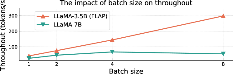
Figure 7: The impact of batch size on throughput. The hardware is the NVIDIA A100-40G.

Conclusion

In this work, we propose FLAP (FLuctuation-based Adaptive Structured Pruning), a retraining-free structured pruning framework explicitly designed for Large Language Models (LLMs). To address the challenges posed by structured pruning, we introduce a novel structured pruning metric, employ adaptive global model compression strategies, and implement robust compensation mechanisms designed to mitigate potential performance losses. Our empirical results affirm that the structured compression model crafted by FLAP can maintain perplexity and zero-shot performance without any retraining. Especially worth noting is the efficacy of FLAP in upholding model performance at both low and medium compression rates. Our work demonstrates that bias compensation can largely replace retraining or parameter efficient fine-tuning (PEFT). We hope that our work contributes to a better understanding of structured pruning and performance recovery of LLMs.

Appendix A A  Detailed Experimental Settings

Models.

We evaluate FLAP on the LLaMA model family (Touvron et al. 2023) and Vicuna-7B model. LLaMA is a set of Transformer-based large language models open-sourced by Meta, mainly including LLaMA-7B/13B/30B/65B. Vicuna is an instruction fine-tuned model based on the LLaMA framework, leveraging user-shared conversations for its training. Given the widespread adoption of these models in the open-source community and their foundational role in numerous applications, their compression performance serves as a significant benchmark. We apply our method to all four LLaMA models to illustrate the fitness of FLAP for different model scales. While our focus is on LLaMA, the versatility of our approach means it can be extended to other Transformer-based LLMs.

Evaluation.

Following previous work on LLM pruning (Ma, Fang, and Wang 2023; Sun et al. 2023), we first evaluate the language modeling capabilities of the pruned model on the WikiText2 (Merity et al. 2016) validation set. We specifically report on the perplexity metric, which gauges a model’s predictive accuracy for the sample set. For a more comprehensive evaluation, we employ the EleutherAI LM Harness, a public evaluation benchmark. With it, we evaluate the model’s zero-shot performance across seven pivotal common sense benchmarks: BoolQ (Clark et al. 2019), PIQA (Bisk et al. 2020), HellaSwag (Zellers et al. 2019), WinoGrande (Sakaguchi et al. 2019), ARC-easy (Clark et al. 2018), ARC-challenge (Clark et al. 2018) and OpenbookQA (Mihaylov et al. 2018). We report both the accuracy of each benchmark and the overall average accuracy.

Baselines.

We compare our method with two previous pruning methods:

• Wanda can be viewed as a continuation of OBD (LeCun, Denker, and Solla 1989) for LLMs, which takes the weight magnitude multiplied by the $\ell_{2}$-norm of the corresponding input activation as the importance score, and prunes locally within the weights corresponding to each output feature of the current linear layer. We generalize Wanda tto structured pruning by counting the $\ell_{2}$-norm of each group of weights within the linear layer as the importance score of the whole group and name it as Wanda-sp.

• LLM-Pruner is the first structured pruning method for LLMs. This method requires the computation of global gradient information and LoRA fine-tuning.

We also attempted to modify SparseGPT (Frantar and Alistarh 2023) to structured pruning, but we fail to obtain reasonable results.

Appendix B B  Implementation Details

Our experiments are performed on an NVIDIA A100 GPU with 40 GB memory. To prune the LLaMA models, we first load them onto GPUs in 16-bit floating-point format. To facilitate the pruning of larger scale models, standardization of the importance metric and threshold filtering are performed uniformly on the CPU, while the remaining procedures (e.g., pruning and recovering) are executed directly on GPUs. For zero-shot tasks, we utilize the evaluation framework available at https://github.com/EleutherAI/lm-evaluation-harness/.

B.1  Wanda for structured pruning

In order to demonstrate that the unstructured pruning methods of existing Large Language Models (LLMs) are not well-suited for structured pruning, we modify the Wanda (Sun et al. 2023) metric to create a structured metric. This adapted metric is designed to align with the characteristics of structured pruning, and it takes the following form:

$$\mathbf{S}^{\ell}_{:,j}=\sum_{i=1}^{row}\left|\mathbf{W}^{\ell}_{ij}\right|\cdot\left\|\mathbf{X}^{\ell}_{j}\right\|_{2}$$ (7)

where $|\cdot|$ represents the absolute value operator, $\|\mathbf{X}_{j}\|_{2}$ evaluates the $\ell_{2}$-norm of $j$-th features aggregated across $N\times L$ different tokens, and the final score is computed by the sum of the product of these two scalar values.

Input: Original model $\mathcal{F}$, calibration samples $\mathcal{D}_{t}$, weights of the original model $\mathbf{W}^{\ell}$, total pruning ratio $p$

Output: Structured pruning mask $\mathbf{M}^{\ell}$, baseline bias $\mathbf{B}^{\ell}_{0}$, model $\mathcal{F^{\star}}$ after pruning and bias compensation

1

2for $\ell\leftarrow 0$ to $len(layers)$ do

3      

4      # Calculate the importance score $\mathbf{S}^{\ell}_{:,j}$ of each column of weight matrix

5      $\mathbf{S}^{\ell}_{:,j}\leftarrow\sum_{n=1}^{N}||\mathbf{X}^{\ell}_{n,j,:}-\overline{\mathbf{X}}^{\ell}_{:,j,:}||_{2}\cdot||\mathbf{W}^{\ell}_{:,j}||_{2}$

6      # Standardized score for each weight to make the current $\mathbf{S}^{\ell}_{a}$ and $\mathbf{S}^{\ell}_{m}$ comparable

7      $\widehat{\mathbf{S}}^{\ell}_{a}=(\mathbf{S}^{\ell}_{a}-\mathbb{E}[\mathbf{S}^{\ell}_{a}])/(\mathbb{E}[[\mathbf{S}^{\ell}_{a}-\mathbb{E}[\mathbf{S}^{\ell}_{a}]]^{2}])^{\frac{1}{2}}$, $\widehat{\mathbf{S}}^{\ell}_{m}=(\mathbf{S}^{\ell}_{m}-\mathbb{E}[\mathbf{S}^{\ell}_{m}])/(\mathbb{E}[[\mathbf{S}^{\ell}_{m}-\mathbb{E}[\mathbf{S}^{\ell}_{m}]]^{2}])^{\frac{1}{2}}$

8# Generate pruning mask $\mathbf{M}^{\ell}$ by ranking $\widehat{\mathbf{S}}$

9$\widehat{\mathbf{S}}\leftarrow{\tt Concat}(\mathbf{S}^{\ell}_{a},\mathbf{S}^{\ell}_{m})$,  $\mathbf{M}^{\ell}\leftarrow{\tt TopKMask}(\widehat{\mathbf{S}},\ p\cdot{\tt Size}(\mathbf{M}))$

10# Use the baseline value $\overline{\mathbf{X}}^{\ell}$ to calculate the bias $\mathbf{B}^{\ell}_{0}$ of Linear layer

11$\overline{\mathbf{X}}^{\ell}_{:,j,:}\leftarrow\frac{1}{NL}\sum_{n=1}^{N}\sum_{k=1}^{L}\mathbf{X}^{\ell}_{n,j,k}$, $\mathbf{B}^{\ell}_{0}\leftarrow((1-\mathbf{M}^{\ell})\odot\mathbf{W}^{\ell})\overline{\mathbf{X}}^{\ell}$, $\mathbf{W}^{\ell}\mathbf{X}^{\ell}\leftarrow(\mathbf{M}^{\ell}\odot\mathbf{W}^{\ell})\mathbf{X}^{\ell}+\mathbf{B}^{\ell}_{0}$

return $\mathcal{F^{\star}}\leftarrow\mathcal{F}_{p}(x|\mathbf{M},\mathbf{W},\mathbf{B}_{0})$

Algorithm 1 FLAP (FLuctuation-based Adaptive Structured Pruning)

B.2  Pseudo Code

The detailed steps of our method are outlined in Algorithm 1. The inputs to FLAP encompass the original model $\mathcal{F}$, calibration samples $\mathcal{D}_{t}$, and overall pruning ratios $p$. The final outputs include the global structured pruning mask $\mathbf{M}^{\ell}$, the baseline bias $\mathbf{B}^{\ell}_{0}$, and the pruned model $\mathcal{F^{\star}}$.

Our approach decomposes the pruning problem for Large Language Models (LLMs) into layer-wise pruning subproblems. In each subproblem, we utilize the calibration data to statistic the input feature information of the corresponding layer and compute the importance score $\mathbf{S}$ using the fluctuation metric. To facilitate the identification of the optimal global compression model structure, we standardize the importance scores of each module in each layer to a standard distribution with a mean of 0 and a variance of 1. Building on this, we merge the importance scores of all layers and modules, then conduct a unified threshold search and to ultimately obtain the global pruning mask. Based on the pruning mask of each layer, we execute the actual pruning of the model and employ the information from the calibration data to introduce additional bias terms, thereby compensating for the reconstruction error of the corresponding layer.

Streaming update.

When counting the information of the input features, we need to estimate the sample mean and sample variance of these features. To minimize repeated calculations and reduce storage, we adopt Welford’s method (Welford 1962) to update the mean and variance in a streaming manner. Specifically, the original sample mean and variance are computed using the following formula:

$$\bar{x}=\frac{1}{n}\sum_{i=1}^{n}x_{i}$$ (8)

$$s^{2}=\frac{1}{n-1}\sum_{i=1}^{n}\left(x_{i}-\bar{x}\right)^{2}$$

In the context of streaming processing, Welford’s method proves to be particularly advantageous as it enables the immediate update of the variance as new samples are received, eliminating the need to recalculate from scratch. This approach is highly efficient, as it not only streamlines data handling but also significantly reduces computational time.

Assuming we have already observed $n$ samples for which we have calculated their mean and variance, when the $n+1$-th sample $x_{n+1}$ arrives, Welford’s method allows us to use the following formulas to seamlessly update the mean $\bar{x}_{n}$ and variance $s_{n}^{2}$:

Update mean: $$\bar{x}_{n+1}=\bar{x}_{n}+\frac{x_{n+1}-\bar{x}_{n}}{n+1}$$ (9)

Update variance: $$s_{n+1}^{2}=\frac{n-1}{n}s_{n}^{2}+\frac{\left(x_{n+1}-\bar{x}_{n}\right)\left(x_{n+1}-\bar{x}_{n+1}\right)}{n+1}$$

Group pruning of attention heads.

In the structured pruning of Transformers, the self-attention module cannot directly prune the rows or columns of weights. Instead, it necessitates structured pruning at the granularity of the ’head’, which is represented by a set of rows or columns of weights. To better align the importance scores between different modules (Self-attn and MLP), we first compute the fluctuation metrics for each column of the weights, doing so separately for each layer and module. We then standardize these metrics, again separately for each layer and module. After standardization, we aggregate the importance scores of neighboring weight columns that correspond to the same head.

In the uniform search across layers and modules, the number of parametric reductions resulting from pruning a self-attention head differs from that resulting from pruning an MLP neuron. To account for this discrepancy, we employ a normalization factor (e.g., 512 / 3). This factor adjusts the importance scores of different modules to be comparable when the same number of elements is removed.

Appendix C C  Additional Experiments

C.1  Zero-shot performance in larger scale

Table 5 presents the zero-shot performance of various downstream tasks with the proposed method applied to the LLaMA-13B model. Our method outperforms the LLM-Pruner, showcasing superior pruning capabilities.

Method	Pruning Ratio	BoolQ	PIQA	HellaSwag	WinoGrande	ARC-e	ARC-c	OBQA	Average
LLaMA-13B	0$\%$	68.47	78.89	76.24	70.09	74.58	44.54	42.00	64.97
LLM-Pruner	20$\%$	67.68	77.15	73.41	65.11	68.35	38.40	42.40	61.79
LLM-Pruner (w/ LoRA)		70.31	77.91	75.16	67.88	71.09	42.41	43.40	64.02
FLAP (Ours)		70.12	77.59	76.01	69.24	72.59	42.56	43.53	64.52

Table 5: Zero-shot performance of the compressed LLaMA-13B. Bold results highlight the best performance. Underscored results denote the second-best performance for each pruning ratio.

C.2  Pruning on Vicuna-7B

In Table 6, we present a direct comparison between FLAP and LLM-Pruner on the Vicuna-7B model, where FLAP demonstrates enhanced performance.

Model	Baseline	Method (20$\%$ Pruning ratio)
		LLM-Pruner	LLM-Pruner w/ LoRA	FLAP
Vicuna-7B	16.11	24.70	18.97	17.99

Table 6: WikiText2 validation perplexity of pruning methods for Vicuna-7B model.

C.3  Different calibration data selection

The selection of calibration data affects the method’s generalization. Table 7 shows that different calibration data suit different downstream tasks, yet the overall average accuracy differences are not significant. Specifically, choosing different calibration datasets, e.g. C4 and WikiText2, results in a fluctuation of about ±1$\%$ in average accuracy for the zero-shot tasks. This phenomenon is also observed in replication experiments with other methods that rely on calibration data, like SparseGPT (Frantar and Alistarh 2023).

Calibration Data	BoolQ	PIQA	HellaSwag	WinoGrande	ARC-e	ARC-c	OBQA	Average
C4	60.21	67.52	52.14	57.54	49.66	29.95	35.60	50.37
Wikitext2	61.04	63.82	43.68	54.93	48.36	30.15	36.31	48.33

Table 7: The impact of different calibration data on generalization ability.

C.4  Generations From Compressed Model

Table 8 and Table 9 present additional examples of the models pruned by our method. We showcase the generation results of both the dense model and the pruned model. Our experiments demonstrate that the pruned LLaMa models with 5.1B and 4.5B parameters, obtained through our pruning approach, are highly effective in retaining general knowledge.

Model	Generated Sentences
LLaMA-7B (baseline)	AI can create a logo in seconds. In the same way, AI can create a new product or service in seconds. The only thing that is missing is the creative mind of a human. This is why I am so excited about this new technology. It’s going to change the world and create a new era of prosperity for all of us.bolds. The best way to get started is to learn the basics of AI. You can do this by reading my book, Artificial Intelligence for Beginners. It is a short book and easy to read. I have also created a video course to help you learn the basics of AI. This is an excellent way to learn the basics of AI. The course is divided into 10 lessons and takes about 2 hours to complete. You can watch the videos on your computer or mobile device. I hope you enjoy the course and learn a lot about AI. If you have any questions, please leave a comment below. Previous articleWhat is AI? – AI Explained Next articleHow to Learn AI – 5 Ways to Learn AI What is AI? – AI Explained AI is a term that is used to describe a wide range of technologies. In this article, I will explain what AI is and… How to Learn AI – 5 …
	What is McDonald’s? McDonald’s is a fast food restaurant that serves hamburgers, french fries, chicken nuggets, salads, milkshakes, soft drinks, and coffee. What is the company’s mission? To provide outstanding quality, service, cleanliness, and value to customers. What is the company’s vision? To be the world’s best quick service restaurant experience by 2015. Who is the CEO? Jim Skinner. How many restaurants does McDonald’s have? 31,000 in 119 countries. What are the company’s core values? Quality, Service, Cleanliness, and Value. What are the company’s strategic objectives? Growth, Innovation, Customer Focus, People, and Financial Discipline. What are the company’s financial objectives? To achieve 10$\%$ revenue growth and 15$\%$ EPS growth by 2015. What are the company’s marketing objectives? To increase customer satisfaction and loyalty by providing quality products and services at a value that customers perceive as good. What are the company’s product/service objectives? To provide a variety of high-quality food and beverages that meet customers’ needs and desires. What are the company’s pricing objectives? To maintain price leadership by …
LLaMA-5.1B (pruned model)	AI can create a logo in seconds. In 2017, the AI company Deepgram was able to create a logo that was indistinguishable from the work of a human designer. In 2018, the same company released a video showing how its logo-creation algorithm was able to replicate the style of the world’s most famous graphic designers, including Saul Aalbersheim, Milton Glaser, Massimo Vigna, Paula Parra, and Paul Rigby. AI is a powerful tool for branding and marketing, but it’s not the only thing that can be used to create a brand. Branding can be done by hand, or it can be done with the help of a branding agency. Branding is an art …
	What is McDonald’s? McDonald’s is the world’s largest fast food chain. It has restaurants in 119 countries and serves over 58 million customers each day. The company’s headquarters are in Oakbrook, Illinois, and it employs over 30,000 people worldwide. What is Mcdonalds? Mcdonalds is a chain of fast food restaurants with a menu of hamburgers, cheeseburgers, quarter pounders with cheese, double cheeseburgers, cheeseburger deluxe, big macs, and other food items. How much does Mcdonalds pay? The average salary for Mcdonalds employees is 20,000 per year. The average salary for Mcdonalds employees in the United States is 20,000.SERTIFIED MCDONALD’S INCORPORATION 1000 WEST 10TH STREET, SAN ANTONIO, TX 78216-3400. What is the phone number at Mcdonalds? The phone number for the corporate headquarters of Mcdonalds is 800-355-4378. This number is used to report food …

Table 8: Generated Examples from the Compressed LLaMA-5.1B by FLAP.

Model	Generated Sentences
LLaMA-7B (baseline)	AI can create a logo in seconds. In the same way, AI can create a new product or service in seconds. The only thing that is missing is the creative mind of a human. This is why I am so excited about this new technology. It’s going to change the world and create a new era of prosperity for all of us.bolds. The best way to get started is to learn the basics of AI. You can do this by reading my book, Artificial Intelligence for Beginners. It is a short book and easy to read. I have also created a video course to help you learn the basics of AI. This is an excellent way to learn the basics of AI. The course is divided into 10 lessons and takes about 2 hours to complete. You can watch the videos on your computer or mobile device. I hope you enjoy the course and learn a lot about AI. If you have any questions, please leave a comment below. Previous articleWhat is AI? – AI Explained Next articleHow to Learn AI – 5 Ways to Learn AI What is AI? – AI Explained AI is a term that is used to describe a wide range of technologies. In this article, I will explain what AI is and… How to Learn AI – 5 …
	What is McDonald’s? McDonald’s is a fast food restaurant that serves hamburgers, french fries, chicken nuggets, salads, milkshakes, soft drinks, and coffee. What is the company’s mission? To provide outstanding quality, service, cleanliness, and value to customers. What is the company’s vision? To be the world’s best quick service restaurant experience by 2015. Who is the CEO? Jim Skinner. How many restaurants does McDonald’s have? 31,000 in 119 countries. What are the company’s core values? Quality, Service, Cleanliness, and Value. What are the company’s strategic objectives? Growth, Innovation, Customer Focus, People, and Financial Discipline. What are the company’s financial objectives? To achieve 10$\%$ revenue growth and 15$\%$ EPS growth by 2015. What are the company’s marketing objectives? To increase customer satisfaction and loyalty by providing quality products and services at a value that customers perceive as good. What are the company’s product/service objectives? To provide a variety of high-quality food and beverages that meet customers’ needs and desires. What are the company’s pricing objectives? To maintain price leadership by …
LLaMA-4.5B (pruned model)	AI can create a logo in seconds. In 2016, Google’s DeepDream AI was able to create a realistic image of a person from a blank canvas. In 2017, DeepMind, Google’s subsidiary, created a robot that played Go chess, which is a game of checkers that humans have played for centuries. This year, we’re going to see the emergence of artificial intelligence that will be able to do things that we have never dreamed of. The most important thing is that we will be able to create a virtual reality, and it will be more real than our physical world. In the next few years, we will see virtual reality, augmented reality, and holographic displays. These will be used in a variety of industries, including the automotive industry, where they will be the primary driver of the next generation of cars. We will also see virtual reality in sports, where the technology will be used to improve the performance of athletes. In the near future, virtual reality will be a part of our everyday lives. In 2017, the world’s first robotic surgery was performed in the U.S. by robotic arms controlled by doctors from more than 2,000 miles away. Robotics are the fastest-growing segment of the robotics industry, and robot-assisted surg…
	What is McDonald’s? McDonald’s is a fast food chain that has over 1, locations worldwide. Its headquarters are in Oak Brook, Illinois, and it is the largest fast food restaurant chain in the world. The company operates in more than countries and employs over 60, people. McDonald’s serves more than million customers every day, which makes it the most popular fast food chain in the world. The company’s revenue in fiscal was billion, and it is the second-largest fast food restaurant chain in the world after Burger King. The company has a large number of restaurants in the United States, but it also has a presence in many other countries, including Canada, the United Kingdom, and Japan. In , the company opened its first restaurant in Japan, and in , it opened its first restaurant in China. In , the company began to serve food in South Korea, and in , it opened its first restaurant in the Middle East. The company also has a large number of franchise locations, which are owned by local businessmen and women. The company is known for its fast food, which is a staple of many diets around the world. The menu includes items such as hamburgers, fried chicken, and burgers, and it has been expanded to include a variety of menu items. The company also sells soft drinks, including Pepsi, Coca Cola …

Table 9: Generated Examples from the Compressed LLaMA-4.5B by FLAP.

References

- Anand et al. (2023) Anand, Y.; Nussbaum, Z.; Duderstadt, B.; Schmidt, B.; and Mulyar, A. 2023. GPT4All: Training an Assistant-style Chatbot with Large Scale Data Distillation from GPT-3.5-Turbo. https://github.com/nomic-ai/gpt4all. Accessed: 2023-08-09.
- Anwar, Hwang, and Sung (2017) Anwar, S.; Hwang, K.; and Sung, W. 2017. Structured pruning of deep convolutional neural networks. ACM Journal on Emerging Technologies in Computing Systems (JETC), 13(3): 1–18.
- Bisk et al. (2020) Bisk, Y.; Zellers, R.; Bras, R. L.; Gao, J.; and Choi, Y. 2020. PIQA: Reasoning about Physical Commonsense in Natural Language. In Thirty-Fourth AAAI Conference on Artificial Intelligence.
- Bommarito and Katz (2022) Bommarito, M.; and Katz, D. M. 2022. GPT Takes the Bar Exam. arXiv:2212.14402.
- Brown et al. (2020) Brown, T. B.; Mann, B.; Ryder, N.; Subbiah, M.; Kaplan, J.; Dhariwal, P.; Neelakantan, A.; Shyam, P.; Sastry, G.; Askell, A.; et al. 2020. Language models are few-shot learners. arXiv:2005.14165.
- Bubeck et al. (2023) Bubeck, S.; Chandrasekaran, V.; Eldan, R.; Gehrke, J.; Horvitz, E.; Kamar, E.; Lee, P.; Lee, Y. T.; Li, Y.; Lundberg, S.; Nori, H.; Palangi, H.; Ribeiro, M. T.; and Zhang, Y. 2023. Sparks of Artificial General Intelligence: Early experiments with GPT-4. arXiv:2303.12712.
- Clark et al. (2019) Clark, C.; Lee, K.; Chang, M.-W.; Kwiatkowski, T.; Collins, M.; and Toutanova, K. 2019. BoolQ: Exploring the Surprising Difficulty of Natural Yes/No Questions. In Proceedings of the 2019 Conference of the North American Chapter of the Association for Computational Linguistics: Human Language Technologies, Volume 1 (Long and Short Papers), 2924–2936. Minneapolis, Minnesota: Association for Computational Linguistics.
- Clark et al. (2018) Clark, P.; Cowhey, I.; Etzioni, O.; Khot, T.; Sabharwal, A.; Schoenick, C.; and Tafjord, O. 2018. Think you have Solved Question Answering? Try ARC, the AI2 Reasoning Challenge. arXiv:1803.05457v1.
- Dettmers et al. (2022) Dettmers, T.; Lewis, M.; Belkada, Y.; and Zettlemoyer, L. 2022. LLM.int8(): 8-bit Matrix Multiplication for Transformers at Scale. In Advances in Neural Information Processing Systems.
- Dettmers et al. (2023) Dettmers, T.; Svirschevski, R.; Egiazarian, V.; Kuznedelev, D.; Frantar, E.; Ashkboos, S.; Borzunov, A.; Hoefler, T.; and Alistarh, D. 2023. SpQR: A Sparse-Quantized Representation for Near-Lossless LLM Weight Compression. arXiv:2306.03078.
- Frantar and Alistarh (2023) Frantar, E.; and Alistarh, D. 2023. SparseGPT: Massive Language Models Can Be Accurately Pruned in One-Shot. arXiv:2301.00774.
- Frantar et al. (2023) Frantar, E.; Ashkboos, S.; Hoefler, T.; and Alistarh, D. 2023. GPTQ: Accurate Post-training Compression for Generative Pretrained Transformers. In International Conference on Learning Representations.
- Gao et al. (2021) Gao, L.; Tow, J.; Biderman, S.; Black, S.; DiPofi, A.; Foster, C.; Golding, L.; Hsu, J.; McDonell, K.; Muennighoff, N.; et al. 2021. A framework for few-shot language model evaluation. Version v0. 0.1. Sept.
- Han, Mao, and Dally (2016) Han, S.; Mao, H.; and Dally, W. J. 2016. Deep compression: Compressing deep neural networks with pruning, trained quantization and Huffman coding. In International Conference on Learning Representations.
- Han et al. (2015) Han, S.; Pool, J.; Tran, J.; and Dally, W. J. 2015. Learning both weights and connections for efficient neural networks. In Advances in Neural Information Processing Systems.
- Hassibi, Stork, and Wolff (1993) Hassibi, B.; Stork, D. G.; and Wolff, G. J. 1993. Optimal brain surgeon and general network pruning. In IEEE International Conference on Neural Networks.
- He and Xiao (2023) He, Y.; and Xiao, L. 2023. Structured Pruning for Deep Convolutional Neural Networks: A survey. arXiv:2303.00566.
- Hinton, Vinyals, and Dean (2015) Hinton, G.; Vinyals, O.; and Dean, J. 2015. Distilling the knowledge in a neural network. arXiv:1503.02531.
- Hu et al. (2021) Hu, E. J.; Shen, Y.; Wallis, P.; Allen-Zhu, Z.; Li, Y.; Wang, S.; Wang, L.; and Chen, W. 2021. Lora: Low-rank adaptation of large language models. arXiv:2106.09685.
- LeCun, Denker, and Solla (1989) LeCun, Y.; Denker, J. S.; and Solla, S. A. 1989. Optimal brain damage. In Advances in Neural Information Processing Systems.
- Ma, Fang, and Wang (2023) Ma, X.; Fang, G.; and Wang, X. 2023. LLM-Pruner: On the Structural Pruning of Large Language Models. Version 3, arXiv:2305.11627.
- Merity et al. (2016) Merity, S.; Xiong, C.; Bradbury, J.; and Socher, R. 2016. Pointer Sentinel Mixture Models. arXiv:1609.07843.
- Mihaylov et al. (2018) Mihaylov, T.; Clark, P.; Khot, T.; and Sabharwal, A. 2018. Can a Suit of Armor Conduct Electricity? A New Dataset for Open Book Question Answering. In EMNLP.
- Mishra et al. (2021) Mishra, A.; Latorre, J. A.; Pool, J.; Stosic, D.; Stosic, D.; Venkatesh, G.; Yu, C.; and Micikevicius, P. 2021. Accelerating sparse deep neural networks. arXiv:2104.08378.
- Molchanov et al. (2017) Molchanov, P.; Tyree, S.; Karras, T.; Aila, T.; and Kautz, J. 2017. Pruning Convolutional Neural Networks for Resource Efficient Inference. In International Conference on Learning Representations.
- Richards (2023) Richards, T. B. 2023. Auto-GPT: An experimental open-source attempt to make GPT-4 fully autonomous. https://github.com/Significant-Gravitas/Auto-GPT. Accessed: 2023-08-09.
- Sakaguchi et al. (2019) Sakaguchi, K.; Bras, R. L.; Bhagavatula, C.; and Choi, Y. 2019. WinoGrande: An Adversarial Winograd Schema Challenge at Scale. arXiv:1907.10641.
- Scao et al. (2022) Scao, T. L.; Fan, A.; Akiki, C.; Pavlick, E.; Ilić, S.; Hesslow, D.; Castagné, R.; Luccioni, A. S.; Yvon, F.; Gallé, M.; et al. 2022. Bloom: A 176b-parameter open-access multilingual language model. arXiv:2211.05100.
- Shi et al. (2023) Shi, D.; Tao, C.; Jin, Y.; Yang, Z.; Yuan, C.; and Wang, J. 2023. Upop: Unified and progressive pruning for compressing vision-language transformers. arXiv:2301.13741.
- Sun et al. (2023) Sun, M.; Liu, Z.; Bair, A.; and Kolter, Z. 2023. A Simple and Effective Pruning Approach for Large Language Models. arXiv:2306.11695.
- Tan and Motani (2020) Tan, C. M. J.; and Motani, M. 2020. Dropnet: Reducing neural network complexity via iterative pruning. In International Conference on Machine Learning, 9356–9366. PMLR.
- Taori et al. (2023) Taori, R.; Gulrajani, I.; Zhang, T.; Dubois, Y.; Li, X.; Guestrin, C.; Liang, P.; and Hashimoto, T. B. 2023. Stanford Alpaca: An Instruction-following LLaMA model. https://github.com/tatsu-lab/stanford˙alpaca. Accessed: 2023-08-09.
- Touvron et al. (2023) Touvron, H.; Lavril, T.; Izacard, G.; Martinet, X.; Lachaux, M.-A.; Lacroix, T.; Rozière, B.; Goyal, N.; Hambro, E.; Azhar, F.; Rodriguez, A.; Joulin, A.; Grave, E.; and Lample, G. 2023. LLaMA: Open and Efficient Foundation Language Models. arXiv:2302.13971.
- Wei et al. (2022) Wei, J.; Tay, Y.; Bommasani, R.; Raffel, C.; Zoph, B.; Borgeaud, S.; Yogatama, D.; Bosma, M.; Zhou, D.; Metzler, D.; Chi, E. H.; Hashimoto, T.; Vinyals, O.; Liang, P.; Dean, J.; and Fedus, W. 2022. Emergent Abilities of Large Language Models. In Transactions on Machine Learning Research.
- Welford (1962) Welford, B. 1962. Note on a method for calculating corrected sums of squares and products. Technometrics, 4(3): 419–420.
- Xia, Zhong, and Chen (2022) Xia, M.; Zhong, Z.; and Chen, D. 2022. Structured Pruning Learns Compact and Accurate Models. In Association for Computational Linguistics (ACL).
- Xiao et al. (2023) Xiao, G.; Lin, J.; Seznec, M.; Wu, H.; Demouth, J.; and Han, S. 2023. SmoothQuant: Accurate and Efficient Post-Training Quantization for Large Language Models. In International Conference on Machine Learning.
- Zafrir et al. (2021) Zafrir, O.; Larey, A.; Boudoukh, G.; Shen, H.; and Wasserblat, M. 2021. Prune once for all: Sparse pre-trained language models. arXiv:2111.05754.
- Zellers et al. (2019) Zellers, R.; Holtzman, A.; Bisk, Y.; Farhadi, A.; and Choi, Y. 2019. HellaSwag: Can a Machine Really Finish Your Sentence? In Proceedings of the 57th Annual Meeting of the Association for Computational Linguistics.
- Zhang et al. (2022) Zhang, S.; Roller, S.; Goyal, N.; Artetxe, M.; Chen, M.; Chen, S.; Dewan, C.; Diab, M.; Li, X.; Lin, X. V.; et al. 2022. OPT: Open pre-trained transformer language models. arXiv:2205.01068.
- Zhou et al. (2021) Zhou, A.; Ma, Y.; Zhu, J.; Liu, J.; Zhang, Z.; Yuan, K.; Sun, W.; and Li, H. 2021. Learning n: m fine-grained structured sparse neural networks from scratch. arXiv:2102.04010.