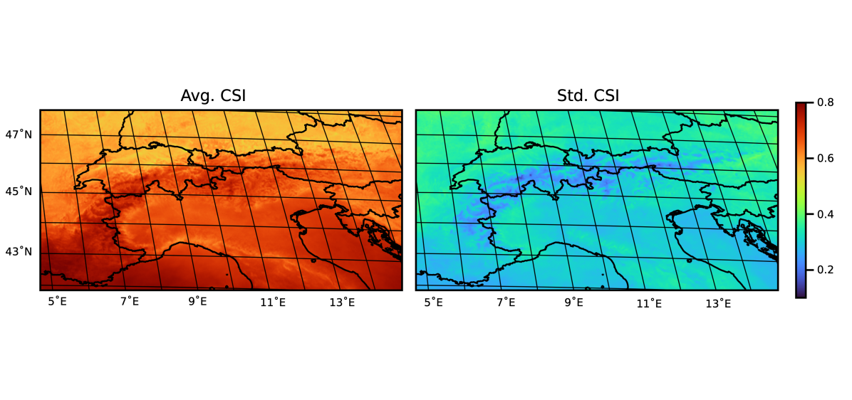
Figure 1: Average and standard deviation at pixel level of CSI values computed on 500 hundred days sampled from the training set. Left panel: average CSI values for the HelioMont covered region. Right panel: average daily CSI standard deviation computed along the time dimension. For every sampled day, the standard deviation along the time dimension is computed for every pixel and then averaged over the 500 hundred days.

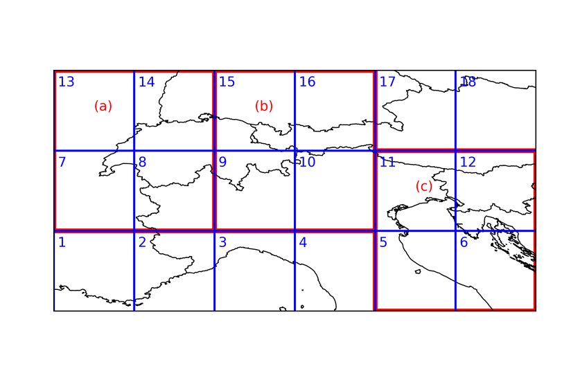
Figure 2: Area covered by the HelioMont dataset [CASTELLI2014] The patches outlined in blue define the cropping applied to create the training set. For the test set we used three $256\times 256$ patches identified by the red borders: (a), (b) and (c).

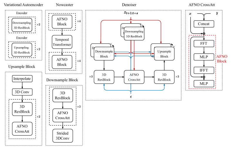
Figure 3: A AFNO-based U-Net architecture is employed in our denoiser, alongside principal blocks integrated into the SHADECast architecture. The symmetrical design of the denoiser includes two downsampling and upsampling blocks. The latent forecast $z_{t+1:t+s}$ undergoes 3-dimensional strided residual blocks to match spatial dimensions with U-Net components, followed by concatenation with the output of AFNO cross attention blocks. In the right panel, $x$ represents the input from the previous layer, and $y$ is the conditioning input. Downsampling is achieved through strided 3D convolutional layers, whereas upsampling utilizes spatial axis interpolation. The 3-dimensional residual blocks consist of two convolutional layers connected by a skip connection.

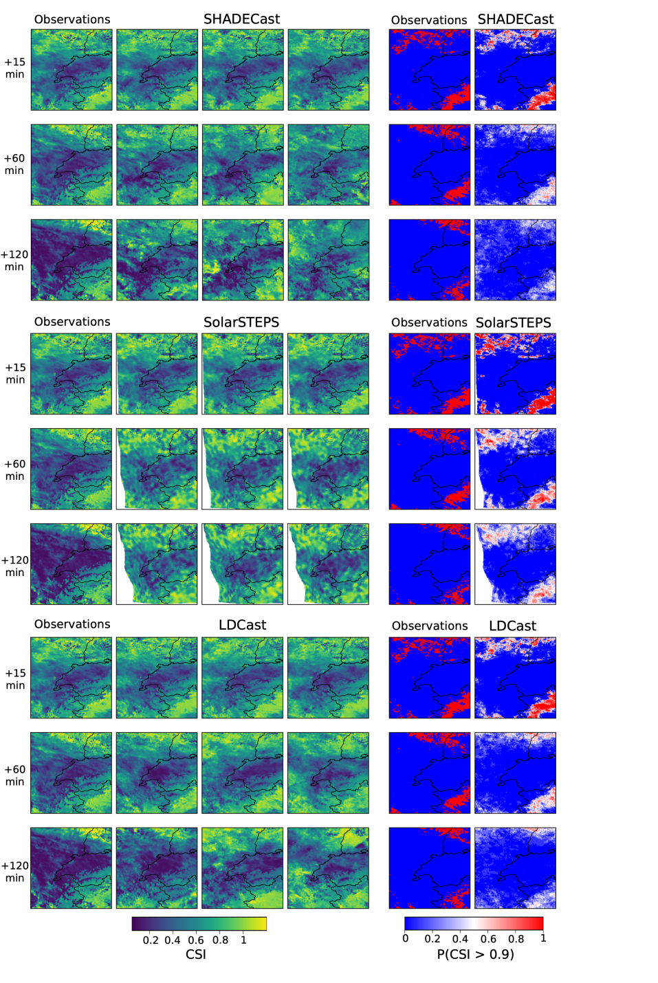
Figure 4: Visualization of generated ensembles at three lead times for SHADECast and two benchmark models. The date (24 Feb. 2016) and starting time (11.45 am) are chosen to show a changing weather situation in which the cloudy surface (blue pixels) increases through the forecast. On the first column, the satellite CSI images are shown (Observations). The second, third and fourth columns show the best, average and worse ensemble members, respectively. The ensemble members are evaluated by their average RMSE over the entire forecast. The last two columns show the ground truth and forecasted probabilities of CSI exceeding $0.9$ (clear-sky). The forecasted region is patch (a) (see Extended Data Patches).

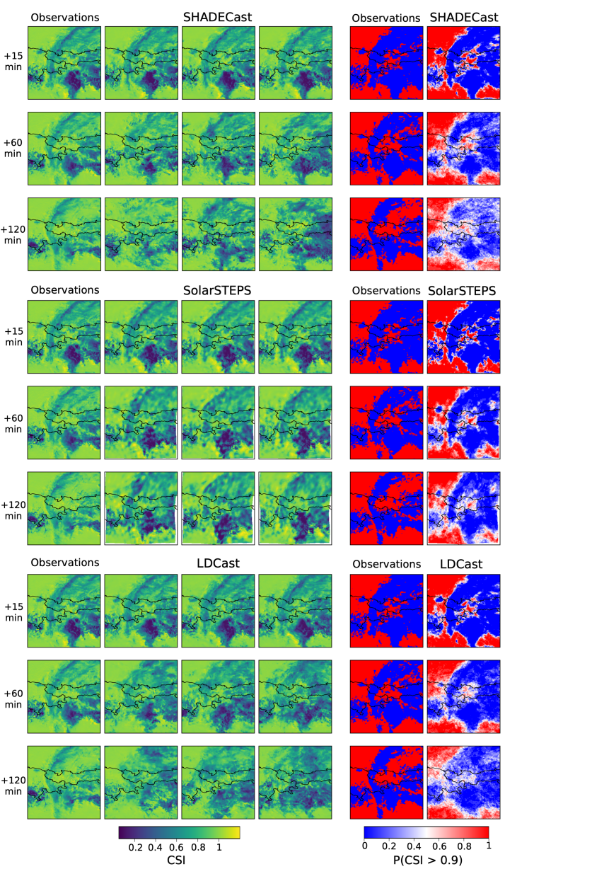
Figure 5: Visualization of generated ensembles at three lead times for SHADECast and two benchmark models. The date (24 Jul. 2015) and starting time (05.30 am) are chosen to show a dissipation example of clouds on the bottom of the region. The figure is structured as Extended Data Test1_Forex. The forecasted region is patch (b) (see Extended Data Patches).

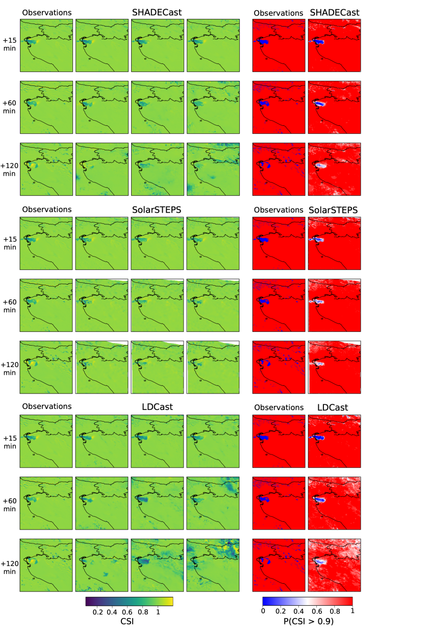
Figure 6: Visualization of generated ensembles at three lead times for SHADECast and two benchmark models. The date (19 Mar. 2016) and starting time (11.15 am) are chosen to show a clear-sky and low variability weather example. The figure is structured as Extended Data Test1_Forex. The forecasted region is patch (c) (see Extended Data Patches).