On order $\Lambda_{\rm QCD}^{2}/m$ renormalons in quarkonium system

Abstract

For the heavy quarkonium system we examine ${\cal O}(\Lambda_{\rm QCD}^{2}/m)$ renormalons, which are expected to be included in the perturbative series of the pole mass and $1/(mr^{2})$ interquark potential. We find indications of existence and cancellation of these renormalons, from examinations of stability and convergence properties of the perturbative series and their resummations, as well as by comparison with the known properties of the ${\cal O}(\Lambda_{\rm QCD})$ renormalons.

TU–1218

1 Introduction

The proper treatment of renormalons in theoretical calculations of QCD plays an important role in recent and near-future high-precision particle physics. For instance, cancellation of renormalons is incorporated in determinations of the fundamental physical constants $m_{b}$, $m_{c}$, $\alpha_{s}(M_{Z})$, $|V_{cb}|$, etc. Renormalons have been actively investigated particularly in the context of heavy quarkonium systems. In fact, the discovery of the cancellation of the ${\cal O}(\Lambda_{\rm QCD})$ renormalons between the twice of the quark pole mass $2m_{\rm pole}$ and the static QCD potential $V_{\rm{QCD}}(r)$ [1, 2, 3] led to a drastic improvement in the predictability of the observables of the heavy quarkonium systems. This cancellation is achieved by expressing the pole mass by a short-distance mass such as the $\overline{\rm MS}$ mass.

In this Letter we focus on the next-to-leading order renormalons in the heavy quarkonium system, i.e., ${\cal O}(\Lambda_{\rm QCD}^{2}/m)$ renormalons. Possible existence of ${\cal O}(\Lambda_{\rm QCD}^{2}/m)$ renormalon in the quark pole mass has been anticipated and discussed. Known properties are as follows [4]. (a) It is induced by the non-relativistic kinetic energy operator $\bm{D}^{2}/(2m)$; (b) It is not forbidden by any symmetry, and parametrically it induces an ${\cal O}(\Lambda_{\rm QCD}^{2}/m)$ uncertainty; (c) It does not appear in the large-$\beta_{0}$ approximation. So far, no strong positive evidence has been reported on the size or effects of this renormalon. The next-to-leading order renormalon contained in $V_{\rm{QCD}}(r)$ is of order $\Lambda_{\rm QCD}^{3}r^{2}$ [5, 6] and no renormalon of order $\Lambda_{\rm QCD}^{2}/m$ is included (since $V_{\rm{QCD}}(r)$ is independent of $m$). The counterpart which cancels the ${\cal O}(\Lambda_{\rm QCD}^{2}/m)$ renormalon of $2m_{\rm pole}$ is expected to be included in the potential $V_{1/r^{2}}(r)\sim-1/(mr^{2})$, which is a part of the non-relativistic Hamiltonian of the quarkonium system. In fact, by naive power counting, we expect the size of the renormalon to be

$$\delta V_{1/r^{2}}~{}\sim~{}\int_{q\lesssim\Lambda_{\rm QCD}}\!\!\!\!d^{3}\bm{q}\,\,\frac{e^{i\bm{q}\cdot\bm{r}}}{m\,q}~{}\sim~{}\frac{{\Lambda_{\rm QCD}}^{2}}{m}\,,$$ (1)

in the case $\Lambda_{\rm QCD}\ll 1/r$, where we used the Fourier integral representation of $V_{1/r^{2}}(r)$. Moreover, it has been pointed out that $V_{1/r^{2}}(r)$ induces anomalously large corrections to the quarkonium spectrum [7], which may be a sign of the ${\cal O}(\Lambda_{\rm QCD}^{2}/m)$ renormalon.

A frequently-used method to investigate renormalons in perturbative QCD is the so-called “large-$\beta_{0}$ approximation” [8]. Unfortunately it is difficult to apply this method to the analysis of the ${\cal O}(\Lambda_{\rm QCD}^{2}/m)$ renormalons of $2m_{\rm pole}$ and $V_{\rm NA}(r)$, since it would involve difficult calculations of bubble-chain insertions to the diagrams shown in Fig. 1. Instead, we use the recently developed method for estimating renormalons, the FTRS [9, 10] and DSRS [11] methods. These methods utilize the property that the renormalons are suppressed in the Fourier space or dual space: By renormalization-group (RG) improvement of the perturbative series in these spaces we can separate the renormalons and the rest, and we can estimate them individually and systematically as more terms of the perturbative series are included; At all orders they coincide with the conventional definition based on the regularized Borel resummation of the perturbative series. Furthermore, for the reason explained below, we restrict the analysis to the “maximally non-abelian (MNA) part” of the perturbative series, corresponding to the part proportional to $C_{F}{C_{A}}^{\!\!n}\alpha_{s}^{n+1}$.

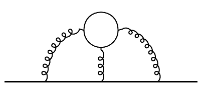
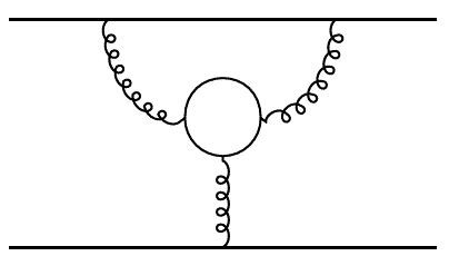
Figure 1: Feynman diagrams relevant to the calculations of the ${\cal O}(\Lambda_{\rm QCD}^{2}/m)$ renormalons of $2m_{\rm pole}$ and $V_{\rm NA}(r)$, respectively, in the large-$\beta_{0}$ approximation. Bubble chain insertions to the gluon propagators of these diagrams need to be computed.

In Sec. 2 we examine $V_{1/r^{2}}$ in the leading-logarithmic (LL) approximation using the FTRS and DSRS methods. Secs. 3 and 4 deal with beyond-the-LL approximation. In Sec. 3 we examine the total energy $2m_{\rm pole}+V_{\rm QCD}+V_{1/r^{2}}$ of the heavy quarkonium system in the fixed order of the perturbative expansion. In Sec. 4 we examine the sizes of the ${\cal O}(\Lambda_{\rm QCD}^{2}/m)$ renormalons as well as the total energy in the FTRS and DSRS methods. We give summary and conclusion in Sec. 5.

2 ${\cal O}(\Lambda_{\rm QCD}^{2}/m)$ renormalon of $V_{\text{NA}}$ in LL approximation

The $1/(mr^{2})$ potential in the non-relativistic Hamiltonian of the quarkonium system is known up to the order $\alpha_{s}^{3}$ [12] within the framework of potential-NRQCD effective field theory [13]. This potential appears first at order $\alpha_{s}^{2}$ and its explicit form (in one operator basis) is given by

$$V_{1/r^{2}}=\frac{\alpha_{s}^{2}}{m_{\rm pole}r^{2}}\Biggl{[}\frac{C_{F}(C_{F}-2C_{A})}{4}+\frac{C_{F}\alpha_{s}}{\pi}\Biggl{\{}\frac{130C_{A}C_{F}-101C_{A}^{2}+(49C_{A}-8C_{F})T_{F}n_{l}}{72}$$

$$~{}~{}~{}~{}~{}~{}~{}~{}+\frac{\beta_{0}}{4}(C_{F}-2C_{A})(\gamma_{E}+\log(\mu r))-\frac{2}{3}C_{A}(C_{A}+2C_{F})(\log 2+2\gamma_{E}+2L_{\rm US})\Biggr{\}}\Biggr{]}\,,$$ (2)

$$\beta_{0}=\frac{11}{3}C_{A}-\frac{4}{3}T_{F}n_{l}\,,~{}~{}~{}~{}~{}~{}~{}L_{\rm US}=\log(\mu_{\rm US}r)\,,$$ (3)

where the color factors are given by $C_{F}=4/3$, $C_{A}=3$ and $T_{F}=1/2$; $n_{l}$ denotes the number of light quark flavors; $\alpha_{s}=\alpha_{s}(\mu^{2})$ denotes the strong coupling constant of the theory with $n_{l}$ quark flavors only in the $\overline{\rm MS}$ scheme.

Because the Hamiltonian itself is not a direct physical observable, there arise two problems in analyzing this potential. One problem is that the $1/(mr^{2})$ potential mixes with other operators in the Hamiltonian under unitary transformations which do not affect physical observables [14]. This feature gives a certain ambiguity to the potential to be analyzed for the renormalon cancellation. The same problem does not occur for the MNA part of the $1/(mr^{2})$ potential (the part proportional to $C_{F}{C_{A}}^{\!\!n}\alpha_{s}^{n+1}$). Below, we analyze the MNA part, since this part remains invariant under unitary transformations and is expected to reflect most vividly the characteristics of the IR renormalons. We call the MNA part of $V_{1/r^{2}}(r)$ as the “non-abelian (NA) potential” for short and denote it by $V_{\rm NA}(r)$.

The other problem is the existence of an IR divergence. $V_{1/r^{2}}$ or $V_{\rm NA}(r)$ is IR divergent at order $\alpha_{s}^{3}$ and beyond. In the above explicit form, the IR divergence has been subtracted in the $\overline{\rm MS}$ scheme in momentum space. Associated to the IR divergence, it has an IR logarithmic term represented by $L_{\rm US}$. This term is canceled by the UV logarithmic term associated with the UV divergence of the ultra-soft (US) contribution. Thus, in a physical observable, $L_{\rm US}$ does not appear but is replaced by logarithms of typical US scales. In the case of the perturbative series of the quarkonium spectrum, the physical logarithmic terms include the “QCD Bethe logarithm” [15] which is analogous to the Bethe logarithm in the Lamb shift. Up to now, there are no known examples where those US contributions give large effects to physical observables; rather their contributions are always with moderate size. Hence, in our analysis below, we either replace $\mu_{\rm US}$ by a typical IR scale and vary it in a reasonable range, or replace the US logarithm by 1 or 0 for the sake of an order-of-magnitude estimate.

Now we estimate the size of the ${\cal O}(\Lambda_{\rm QCD}^{2}/m)$ renormalon of the NA potential using the FTRS method and the LL approximation. Then we demonstrate that the convergence of the perturbative series of the NA potential improves by subtraction of the renormalon.

The FTRS method utilizes the fact that IR renormalons are suppressed by Fourier transformation. As a result, in momentum space convergence is expected to be good. For this reason, it would make sense to approximate the NA potential in momentum space by its LL approximation. Thus, we set

$$\tilde{V}_{\text{NA}}^{\text{LL}}(q) =-\frac{\pi^{2}C_{A}C_{F}}{m_{\text{pole}}q}{\alpha_{s}(q^{2})}^{2}$$ (4)

$$\simeq-\frac{\pi^{2}C_{A}C_{F}}{m\,q}\sum_{n=0}^{\infty}(n+1)\left[\frac{\beta_{0}}{4\pi}\log\biggl{(}\frac{\mu^{2}}{q^{2}}\biggr{)}\right]^{n}\alpha_{s}(\mu^{2})^{n+2}\,,$$

where (only in this section) $\alpha_{s}(q^{2})=4\pi/[\beta_{0}\log(q^{2}/\Lambda_{\overline{\rm MS}}^{2})]$ denotes the one-loop running coupling constant and we set $n_{l}=0$ to take the MNA part. Within our approximation it does not make a difference whether we use the pole mass $m_{\rm pole}$ or the $\overline{\rm MS}$ mass $m\equiv m_{\overline{\rm MS}}(m_{\overline{\rm MS}})$, and we use the latter in the second line. The NA potential in position space is obtained by inverse Fourier transformation of each term of the series expansion in $\alpha_{s}(\mu^{2})$:

$$V_{\text{NA}}^{\text{LL}} =\sum_{n=0}^{\infty}C_{n+1}\alpha_{s}(\mu^{2})^{n+2}\,,$$ (5)

where

$$C_{n+1} =-\frac{\pi^{2}C_{A}C_{F}}{m}{\biggl{(}\frac{\beta_{0}}{4\pi}\biggr{)}}^{n}\int\frac{d^{3}\bm{q}}{(2\pi)^{3}}\frac{e^{i\bm{q}\cdot\bm{r}}}{q}(n+1)\left[\log\left(\frac{\mu^{2}}{q^{2}}\right)\right]^{n}.$$ (6)

The Borel transform of $V_{\text{NA}}^{\text{LL}}$ is given by

$$B_{V_{\rm NA}^{\rm LL}}(u)=\sum_{n=0}^{\infty}\frac{C_{n+1}}{(n+1)!}\left(\frac{4\pi u}{\beta_{0}}\right)^{n+1}=-\frac{4\pi^{3}C_{A}C_{F}}{m\beta_{0}}u\int\frac{d^{3}\bm{q}}{(2\pi)^{3}}\frac{e^{i\bm{q}\cdot\bm{r}}}{q}\left(\frac{\mu^{2}}{q^{2}}\right)^{u}$$

$$~{}~{}~{}~{}~{}~{}~{}~{}~{}=-\frac{2\pi^{3/2}C_{A}C_{F}}{m\beta_{0}r^{2}}\,\left(\frac{\mu^{2}r^{2}}{4}\right)^{u}\hskip 3.0pt\cfrac{u\,\Gamma(1-u)}{\Gamma(\frac{1}{2}+u)}.$$ (7)

Thus, there are poles at $u=1,2,3,\cdots$ in the Borel plane. The standard prescription for the Borel resummation is to regularize the inverse Borel transform by deforming the integral contour of the Borel integral into the upper or lower half $u$-plane. The size of the ${\cal O}(\Lambda_{\rm QCD}^{2}/m)$ renormalon is defined as the imaginary part of the regularized Borel integral around $u=1$. Hence, it can be calculated from the residue of the pole at $u=1$ as

$$[\delta V_{\text{NA}}^{\text{LL}}]_{u=1}^{\mathrm{Borel}} =\frac{2\pi}{i\beta_{0}}\oint_{-C_{1}}du\left(-\frac{2\pi^{3/2}C_{A}C_{F}}{m\beta_{0}r^{2}}\right)\left(\frac{\mu^{2}r^{2}}{4}\right)^{u}\hskip 3.0pt\cfrac{\Gamma(2-u)}{\Gamma(\frac{1}{2}+u)}\frac{u}{1-u}e^{-\tfrac{4\pi}{\beta_{0}\alpha_{s}}u}$$ (8)

$$=-\frac{4\pi^{3}C_{A}C_{F}}{{\beta_{0}}^{2}}\frac{{\Lambda_{\overline{\mathrm{MS}}}}^{2}}{m}.$$

Thus, the $u=1$ renormalon of the NA potential is independent of $r$.

In the FTRS method, there is a shortcut to calculate the same quantity (regularized Borel resummation) bypassing the Borel transform. In the inverse Fourier transformation, we deform the integral path to circumvent the pole of $\alpha_{s}(q^{2})$. Then the renormalon can be extracted as the imaginary part of the regularized inverse Fourier integral. Thus,

$$[\delta V_{\text{NA}}^{\text{LL}}]^{\text{FTRS}}=-\frac{\pi C_{A}C_{F}}{2mr}\oint_{C}\frac{dq}{2\pi i}\sin(qr)\alpha_{s}(q^{2})^{2}$$

$$~{}~{}~{}~{}~{}~{}~{}~{}~{}~{}~{}~{}~{}~{}~{}~{}=-\frac{\pi C_{A}C_{F}}{2mr}\oint_{C}\frac{dq}{2\pi i}\left[qr-\frac{1}{6}(qr)^{3}+\cdots\right]\alpha_{s}(q^{2})^{2}\,,$$ (9)

$$[\delta V_{\text{NA}}^{\text{LL}}]^{\text{FTRS}}_{u=1}=-\frac{\pi C_{A}C_{F}}{2m}\oint_{C}\frac{dq}{2\pi i}\,q\,\alpha_{s}(q^{2})^{2}=-\frac{4\pi^{3}C_{A}C_{F}}{{\beta_{0}}^{2}}\frac{{\Lambda_{\overline{\mathrm{MS}}}}^{2}}{m}\,,$$ (10)

where $C$ is the loop surrounding the pole of $\alpha_{s}(q^{2})$ at $q=\Lambda_{\overline{\rm MS}}$. The linear term in the expansion of $\sin(qr)$ is taken to obtain the $u=1$ renormalon. The result in eq. (10) indeed matches the calculation by the Borel resummation method in eq. (8).

The asymptotic behavior of the perturbative series induced by the $u=1$ renormalon can be extracted from the pole at $u=1$ of the Borel transform in eq. (7) as

$$B_{V_{\rm NA}^{\rm LL}}(u)\sim-\frac{2\pi^{3/2}C_{A}C_{F}}{m\beta_{0}r^{2}}\,\frac{\mu^{2}r^{2}}{4}\,\cfrac{1}{\Gamma({3}/{2})}\,\frac{u}{1-u}\ =-\frac{\pi C_{A}C_{F}}{m\beta_{0}}\mu^{2}\sum_{n=0}^{\infty}u^{n+1}.$$ (11)

Therefore, the order ${\alpha_{s}^{n+2}}$ term of $V^{\text{LL}}_{\text{NA}}$ behaves asymptotically as

$$V_{\text{NA}}^{\text{LL},(n)} \sim-\frac{C_{A}C_{F}{\alpha_{s}}^{2}}{4m}\mu^{2}\left(\frac{\beta_{0}\alpha_{s}}{4\pi}\right)^{n}(n+1)!.$$ (12)

This $r$-independent (constant-potential-like) behavior represents the contribution from the $u=1$ renormalon. Fig. 2(a) shows the truncated perturbative expansion of the NA potential in the LL approximation [eq. (5)], and Fig. 2(b) shows the potential after subtracting the renormalon contribution eq. (12). Each line represents the NA potential up to order ${\alpha_{s}^{N+2}}$, with the input parameters $\mu=3$ GeV, $\Lambda_{\overline{\rm MS}}=0.298$ GeV, $n_{l}=0$, and $m=4.19$ GeV [$\alpha_{s}(\mu^{2})=0.247$].

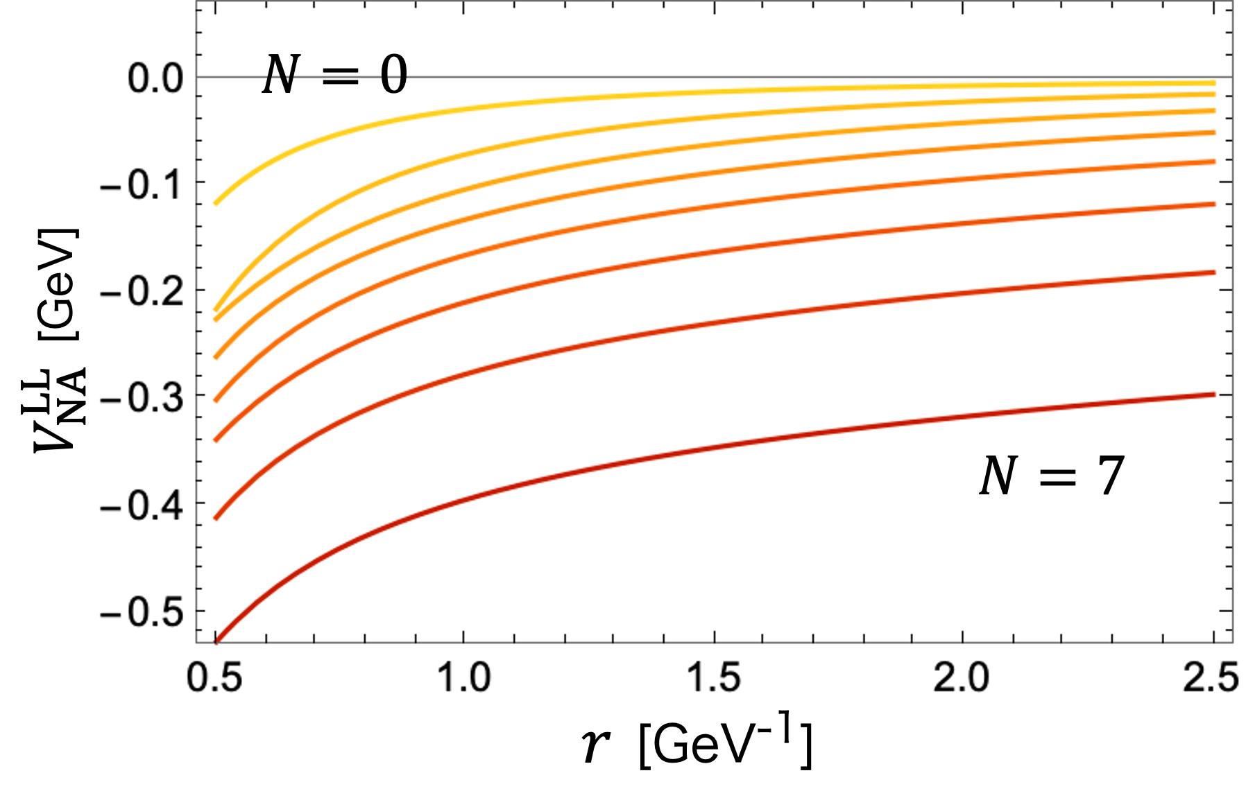
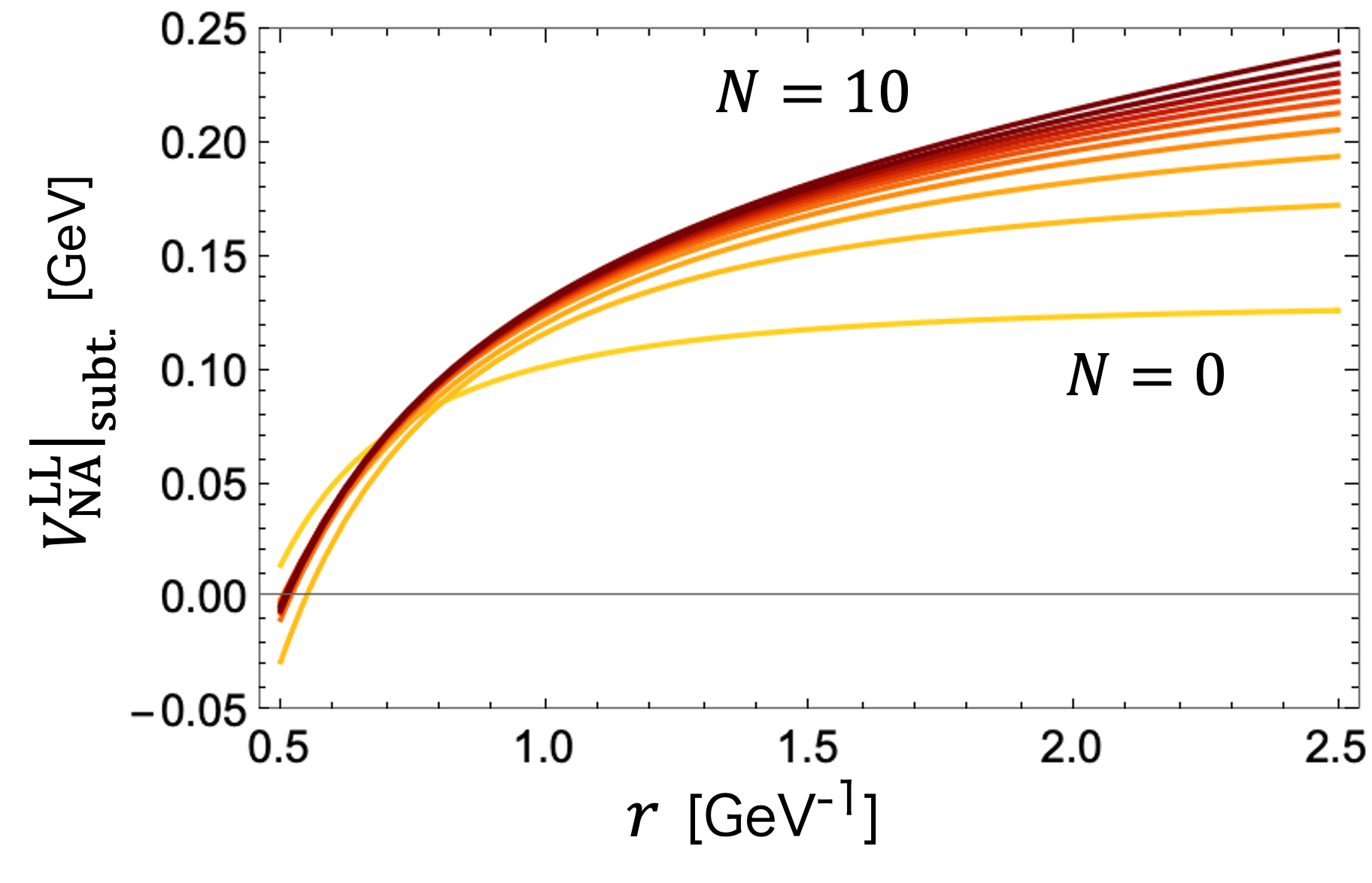
        (a)                                                           (b) 

Figure 2: (a) NA potential in the LL approximation by the FTRS method, expanded in $\alpha_{s}(\mu)$ and truncated at order ${\alpha_{s}^{N+2}}$. (b) The same potential after subtraction of the $u=1$ renormalon contributions. Note that the scale of the vertical axis in (b) is magnified by a factor of two compared to (a).

In Fig. 2(a), as the perturbative order increases, the potential shifts downwards almost by a constant independent of $r$, indicating a lack of convergence by the renormalon contributions [cf., eq. (12)]. On the other hand, in Fig. 2(b), after subtracting the $u=1$ renormalon contributions, the convergence is notably improved. This demonstrates that removing the $u=1$ renormalon enhances the convergence of the perturbative expansion. These features are qualitatively similar to the behaviors of the QCD potential before and after subtraction of the ${\cal O}(\Lambda_{\rm QCD})$ ($u=1/2$) renormalon. (See Figs. 11 of Ref. [16].)

Next, we use the DSRS method to calculate the renormalon of $V_{\text{NA}}^{\text{LL}}(r)$ defined by eqs. (5) and (6). While at all orders the DSRS method gives the same result as the regularized Borel resummation or the FTRS method, its systematic improvement is different from the FTRS method as higher-order terms are included. We choose the parameters of the DSRS method as $(a,u^{\prime})=(1,-1)$ which suppress the renormalons at $u=1,2,3,\cdots$ in the dual space. Following the prescription of Ref. [11], we obtain

$$V_{\text{NA}}^{\text{LL}}(r) =\int_{0}^{\infty}dp^{2}\,e^{-r^{2}p^{2}}\,\,\overline{V}_{\text{NA}}^{\text{LL}}(p^{2})\,,$$ (13)

where the NA potential in the dual space is given by

$$\overline{V}_{\text{NA}}^{\text{LL}}(p^{2})=-\frac{2\pi C_{A}C_{F}}{\beta_{0}m}\sum_{n=0}^{\infty}(n+1)!\,\tilde{a}_{n+1}\,\left(\frac{\beta_{0}}{4\pi}\right)^{n+1}\alpha_{s}(p^{2})^{n+2}\,,$$ (14)

$$\sum_{n=0}^{\infty}\tilde{a}_{n+1}u^{n+1}=\frac{u\,\Gamma(1+u)}{\Gamma(1+2u)}\,.$$ (15)

After truncating the series expansion in eq. (14) at an arbitrary order, we deform the integral path of eq. (13) into the upper or lower-half complex $p^{2}$ plane to circumvent the pole of $\alpha_{s}(p^{2})$. Similarly to the FTRS method, the size of the $u=1$ renormalon is obtained as

$$[\delta V^{\text{LL}}_{\text{NA}}]^{\text{DSRS}}_{u=1} =-\frac{8\pi^{3}C_{A}C_{F}}{{\beta_{0}}^{2}m}\sum_{n=0}^{\infty}\tilde{a}_{n+1}(n+1)!\,\oint_{C}\frac{dp^{2}}{2\pi i}\,\frac{1}{[\log(p^{2}/{\Lambda_{\overline{\mathrm{MS}}}}^{2})]^{n+2}}$$ (16)

$$=-\frac{8\pi^{3}C_{A}C_{F}}{{\beta_{0}}^{2}}\frac{{\Lambda_{\overline{\mathrm{MS}}}}^{2}}{m}\sum_{n=0}^{\infty}\tilde{a}_{n+1}.$$

The sum over $n$ converges. By setting $u=1$ in eq. (15), we find $\sum_{n=0}^{\infty}\tilde{a}_{n+1}=\frac{1}{2}$ and the previous result is reproduced.

Let us examine how the size of the renormalon obtained by the DSRS method converges towards the result of the Borel resummation or the FTRS method. Fig. 3(a) compares the values obtained by truncating the summation in eq. (16) at $n=k$ with the $u=1$ renormalon calculated by the FTRS method (normalized to unity). At low orders, the truncated sum oscillates rather rapidly. As the order increases, the sum converges towards the value of FTRS slowly. From the order $n=7$ the truncated sum starts to approximate the FTRS value with better than 10 per cent accuracy. For comparison, Fig. 3(b) shows the similar calculation of the $u=1/2$ renormalon in the QCD potential in the LL approximation using the DSRS method. The size of the $u=1/2$ renormalon is also normalized to unity. Note that the vertical-axis scales differ by a factor of 4 between the two figures. It can be observed that the convergence speed of the $u=1$ renormalon in $V^{\text{LL}}_{\text{NA}}$ is considerably slower compared to the $u=1/2$ renormalon of the QCD potential.

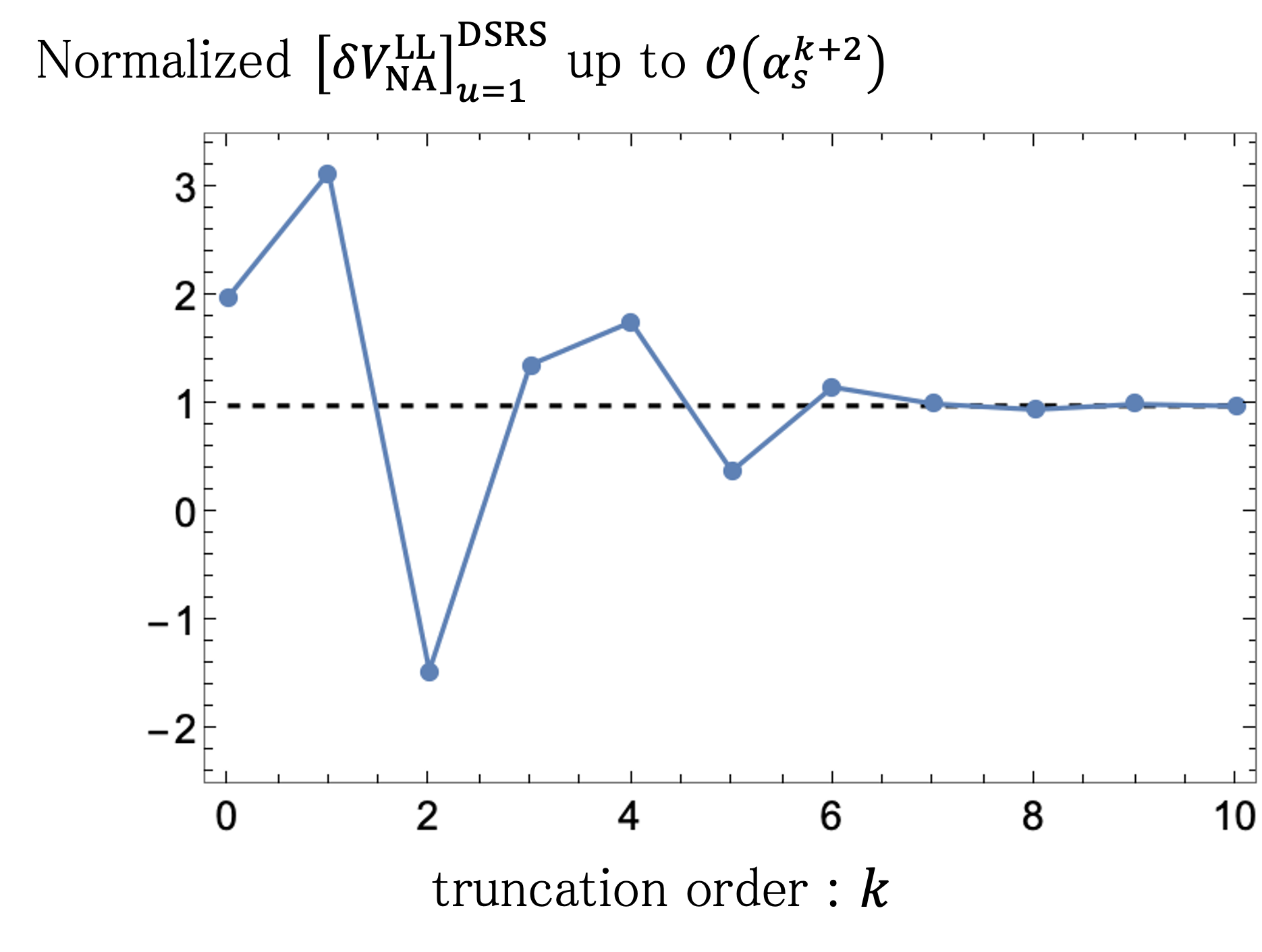
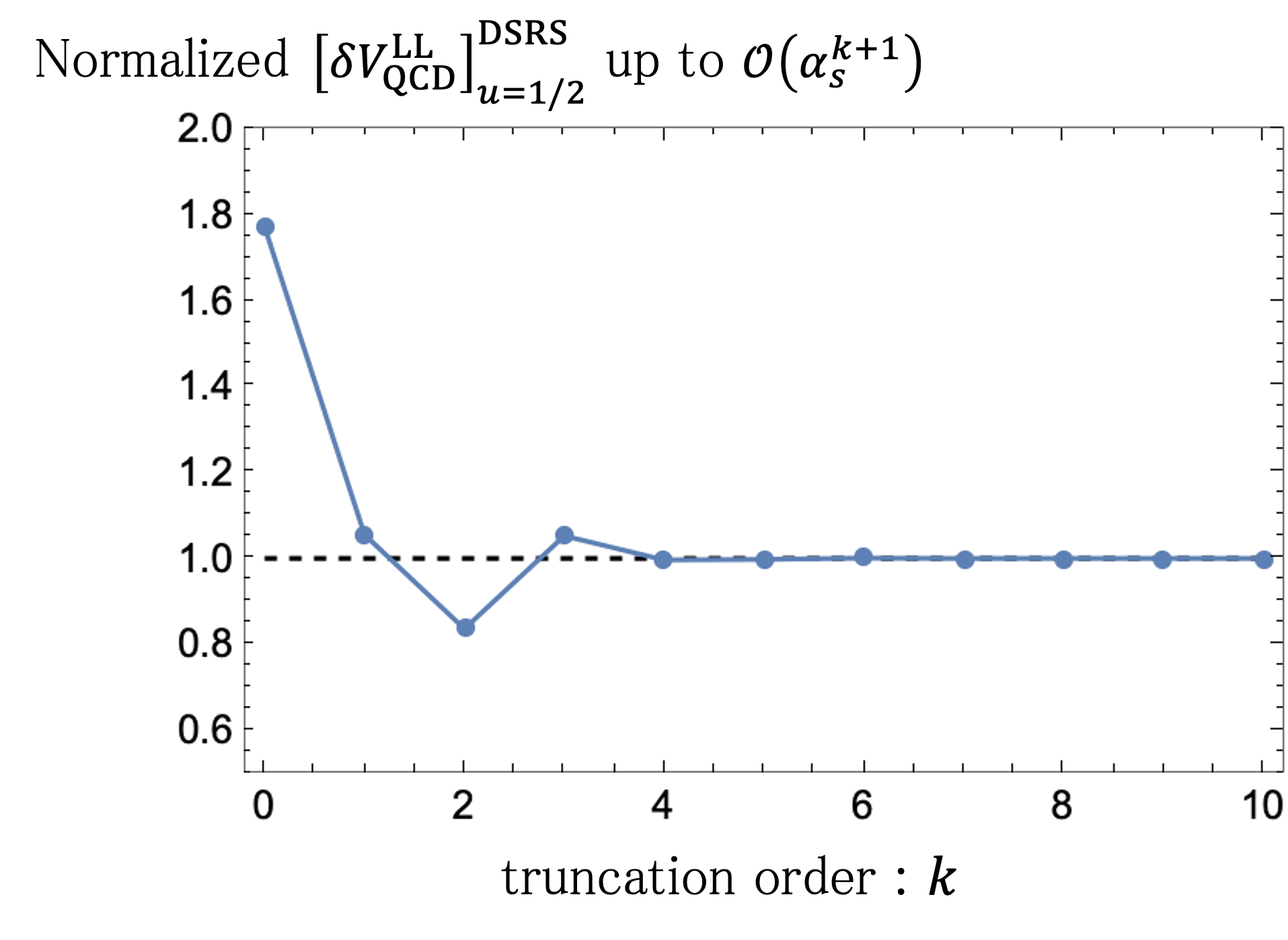
        (a)                                                           (b) 

Figure 3: (a) Size of the $u=1$ renormalon of $V_{\rm NA}^{\rm LL}$ in the DSRS method as we vary the truncation order. (b) Size of the $u=1/2$ renormalon of $V_{\rm QCD}^{\rm LL}$ in the DSRS method as we vary the truncation order. Both series are normalized by the exact values. Note that the scale of the vertical axis in (b) is magnified by a factor of 4 compared to (a).

It can be shown that the expansion coefficients of the $u=u_{*}$ renormalon in the DSRS method includes the factor $u_{*}^{n}$ as $n$ is varied. Hence, in general the convergence tends to become worse as the renormalon is located further away from the origin in the Borel plane.

We have also examined the real part of the resummed potential $V_{\rm NA}^{\rm LL}$ in the FTRS and DSRS methods. The FTRS method gives the Borel resummed potential in the principal-value (PV) prescription and the DSRS method gives a series which converges to it, with our current construction of the potential. The former potential approximates well the $N=7$ truncated potential in Fig. 2(b) (up to an additive constant) in the displayed range, which corresponds to the most convergent line in this figure (truncation at the minimal term). This feature is consistent with the similar property observed for the QCD potential [17]. For the DSRS potential, the convergence is fairly slow in the displayed range. The convergence is better at smaller $r$. More explicitly, evidently converging behavior can be seen only at $r\lesssim 1~{}{\rm GeV}^{-1}$ and for $k\geq 8$. We have to calculate up to higher $k$ to observe a sign of convergence at larger $r$. On the other hand, we observe a better convergence at smaller distances $r<0.5~{}{\rm GeV}^{-1}$.

It is difficult to perform a similar analysis for the $u=1$ renormalon of the pole mass. This is because the $u=1$ renormalon has a subleading structure $\alpha_{s}^{2}\times[\beta_{0}\alpha_{s}\log(\mu/m)]^{n}$, which resides in between the more dominant leading logarithmic structure $\alpha_{s}\times[\beta_{0}\alpha_{s}\log(\mu/m)]^{n}$, and it is difficult to extract the $u=1$ renormalon as clearly as the NA potential. Instead we will perform a more involved analysis in Sec. 4 to assess the $u=1$ renormalon of the pole mass.

3 Beyond LL approximation: Fixed-order analysis of $2m_{\rm pole}$, $V_{\rm QCD}$ and $V_{\rm NA}$

In this section we examine the perturbative series of the total energy of the quarkonium system, $E_{\text{tot}}=2m_{\rm pole}+V_{\rm QCD}+V_{\rm NA}$, and discuss cancellation of renormalons among $2m_{\rm pole}$, $V_{\rm QCD}$ and $V_{\rm NA}$. We examine the MNA part of their exact perturbative expansions in $\alpha_{s}(\mu^{2})$ up to order $\alpha_{s}^{3}$ (fixed-order analysis).

Formally at all orders of perturbative expansion, the dependence of an observable on the renormalization scale $\mu$ disappears. Therefore, if the perturbative series converges, $\mu$ dependence decreases as the order of the perturbative expansion increases. This is not necessarily the case if the perturbative expansion shows poor convergence. In this way, convergence and stability with respect to the scale $\mu$ of the perturbative expansion are closely related. Below, we examine the $\mu$ dependence of the total energy $E_{\text{tot}}$ and consider the effects of renormalon cancellations.

It is believed that, in the quarkonium system, the $u=1/2$ renormalons cancel between $2m_{\rm pole}$ and $V_{\rm QCD}$. We consider it plausible that also the $u=1$ renormalons cancel out in the MNA part of the entire expression of $E_{\text{tot}}=2m_{\text{pole}}+V_{\text{QCD}}+V_{\text{NA}}$. Since the $u=1$ renormalon is subdominant, to observe the effects of the cancellation of this renormalon, it is necessary to cancel the dominant $u=1/2$ renormalons. To clarify the role of each renormalon contribution, we compare the following three cases: (I) $E_{\text{pole}}=2m_{\rm pole}+V_{\rm QCD}+V_{\rm NA}$ without rewriting $m_{\rm pole}$, (II) $E_{{1/r}}=2m_{\rm pole}+V_{\rm QCD}$ after rewriting $m_{\rm pole}$ by the $\overline{\rm MS}$ mass $m$, (III) $E_{\text{full}}=2m_{\rm pole}+V_{\rm QCD}+V_{\rm NA}$ after rewriting $m_{\rm pole}$ by the $\overline{\rm MS}$ mass $m$. It is understood that the MNA part is taken, and in addition we also retain the order $\alpha_{s}^{0}$ term ($2m_{\rm pole}$ in $E_{\text{pole}}$ or $2m$ in $E_{1/r}$, $E_{\text{full}}$) for convenience. We expect that the following renormalons remain uncanceled in each case: (I) ${\cal O}(\Lambda_{\rm QCD})$ and ${\cal O}(\Lambda_{\rm QCD}^{2}/m)$, (II) ${\cal O}(\Lambda_{\rm QCD}^{2}/m)$, (III) None, up to $u=1$.

In the cases (II) and (III) we use the MNA part of the pole mass expressed by the $\overline{\rm MS}$ mass [18],

$$m_{\rm pole}^{\rm MNA}=m\,\Biggl{[}1+\frac{C_{F}\alpha_{s}(m^{2})}{\pi}\biggl{\{}1+\frac{C_{A}\alpha_{s}(m^{2})}{\pi}\left(\frac{1111}{384}-\frac{\pi^{2}}{12}+\frac{\pi^{2}}{4}\log 2-\frac{3}{8}\zeta(3)\right)$$

$$~{}~{}~{}~{}~{}~{}~{}~{}~{}~{}~{}~{}~{}~{}+\Bigl{(}\frac{C_{A}\alpha_{s}(m^{2})}{\pi}\Bigr{)}^{2}\biggl{(}\frac{1322545}{124416}+\frac{1955\pi^{2}}{3456}+\frac{179\pi^{4}}{3456}+\frac{115\pi^{2}}{72}\log 2-\frac{11\pi^{2}}{36}\log^{2}2$$

$$~{}~{}~{}~{}~{}~{}~{}~{}~{}~{}~{}~{}~{}~{}~{}~{}~{}~{}~{}~{}~{}~{}~{}~{}~{}-\frac{11}{72}\log^{4}2-\frac{11}{3}\rm{Li}_{4}\Bigl{(}\frac{1}{2}\Bigr{)}-\frac{1343}{288}\zeta(3)-\frac{51\pi^{2}}{64}\zeta(3)+\frac{65}{32}\zeta(5)\biggr{)}\biggr{\}}\Biggr{]}\,.$$ (17)

We re-emphasize that $\alpha_{s}$ denotes the coupling constant of the theory with $n_{l}$ quark flavors only. For $V_{\rm NA}$ we use the MNA part of eq. (2). The MNA part of the QCD potential is given by [19]

$$V_{\rm QCD}^{\rm MNA}=-\frac{C_{F}\alpha_{s}(r^{-2})}{r}\Biggl{[}1+\frac{C_{A}\alpha_{s}(r^{-2})}{\pi}\left(\frac{31}{36}+\frac{11}{6}\gamma_{E}\right)$$

$$~{}~{}~{}~{}~{}~{}~{}~{}~{}~{}~{}~{}~{}~{}+\Bigl{(}\frac{C_{A}\alpha_{s}(r^{-2})}{\pi}\Bigr{)}^{2}\biggl{(}\frac{4343}{2592}+\frac{247}{54}\gamma_{E}+\frac{121}{36}\gamma_{E}^{2}+\frac{229\pi^{2}}{432}-\frac{\pi^{4}}{64}+\frac{11}{24}\zeta(3)\biggr{)}\Biggr{]}\,.$$ (18)

We rewrite $\alpha_{s}(m^{2})$ and $\alpha_{s}(r^{-2})$ by $\alpha_{s}(\mu^{2})$ using the two-loop relation and re-expand the perturbative series by $\alpha_{s}(\mu^{2})$, in which we set $n_{l}=0$ to maintain consistency with the MNA part.

Using the above expressions, we compare the $\mu$ dependences of $E_{\text{pole}}$, $E_{1/r}$ and $E_{\text{full}}$ in Figs. 4(a) and (b). The input parameters are taken as $\alpha_{s}(2\,{\rm GeV})=0.3$, $m_{\rm pole}=5$ GeV in $E_{\text{pole}}$, and $m=4.19$ GeV in $E_{1/r}$ and $E_{\text{full}}$. We vary $\mu_{\rm US}=0.5$ GeV and $1$ GeV in $E_{\text{full}}$. The interquark distance $r$ is fixed at $0.6~{}\text{GeV}^{-1}$ and $1~{}\text{GeV}^{-1}$ in Figs. 4(a) and (b), respectively.

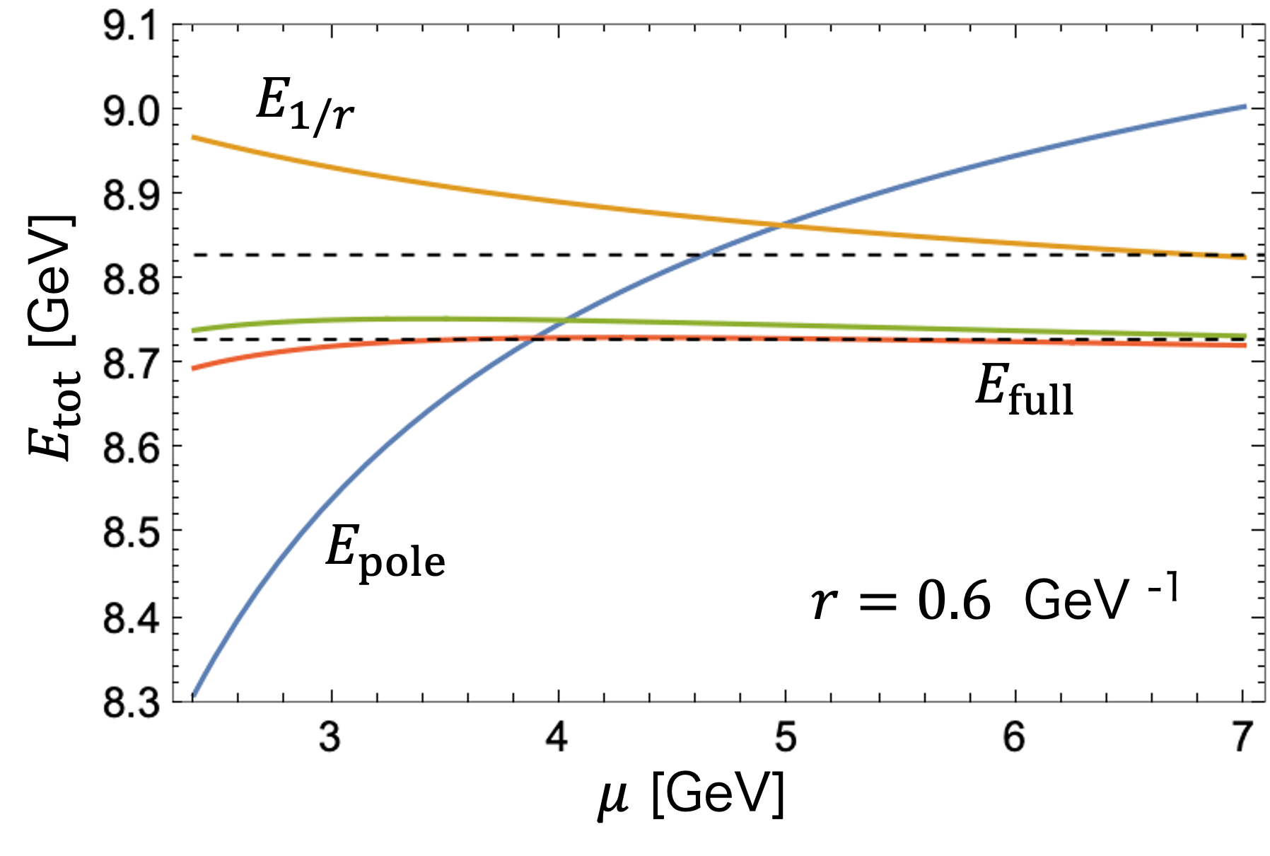
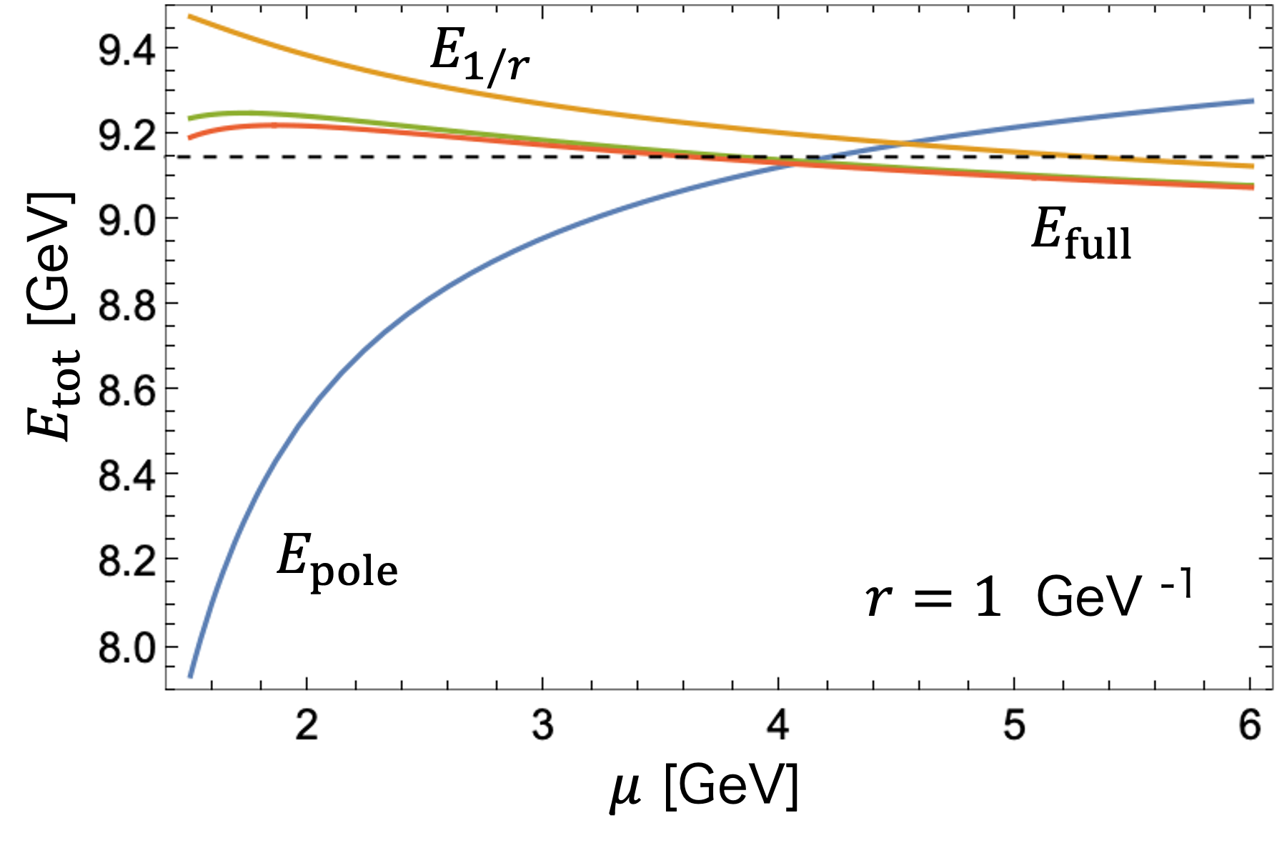
        (a)                                                           (b) 

Figure 4: The total energies $E_{\text{pole}}$, $E_{1/r}$ and $E_{\text{full}}$ vs. $\mu$ at (a) $r=0.6~{}\text{GeV}^{-1}$, (b) $r=1~{}\text{GeV}^{-1}$. The green (red) line represents $E_{\text{full}}$ with $\mu_{\rm US}=0.5~{}{\rm GeV}$ ($1~{}{\rm GeV}$). Horizontal dashed lines are shown as a guide.

We observe that the $\mu$ dependence decreases in the order $E_{\text{pole}}$, $E_{1/r}$ and $E_{\text{full}}$. This is reasonable with regard to the expectation that the $u=1/2$ and $u=1$ renormalons get canceled in this order. This order of the $\mu$ dependence of the three total energies is unchanged for $0.5~{}{\rm GeV}^{-1}\lesssim r\lesssim 2.5~{}{\rm GeV}^{-1}$. At shorter distances, however, the order of $\mu$ dependence between $E_{1/r}$ and $E_{\text{full}}$ is reversed and the $\mu$ dependence of $E_{1/r}$ becomes the smallest. These features agree with the following consideration. The effects of the renormalons are expected to be more prominent at IR, so that the ordering of the $\mu$ dependence according to the expected residual renormalons would be most naturally realized at larger $r$. On the other hand, at short distances $r\ll\Lambda_{\overline{\rm MS}}^{-1}$, $V_{\rm QCD}$ and $V_{\rm NA}$ are mostly perturbative. Hence, $V_{\rm NA}\propto 1/r^{2}$ is most enhanced and its $\mu$ dependence is also magnified at the same time. This explains why at shorter distances the order of $\mu$ dependence between $E_{1/r}$ and $E_{\text{full}}$ is reversed.

Let us fix $\mu$ to the scale where $E_{\text{full}}$ becomes least sensitive to $\mu$ (the minimal sensitivity scale) and compare the perturbative series of the three total energies. For $r=0.6~{}{\rm GeV}^{-1}$, $dE_{\text{full}}/d\mu$ vanishes at $\mu=4.28$ GeV, where the perturbative series are given by

$$E_{\text{pole}}=10.00-0.447-0.358-0.423\hskip 10.0pt\text{GeV}\,,$$ (19)

$$E_{1/r}\,\,=8.380+0.268+0.150-0.085\hskip 10.0pt\text{GeV}\,,$$ (20)

$$E_{\rm full}\,\,=8.380+0.268+0.096-0.012\hskip 10.0pt\text{GeV}\,.$$ (21)

We set $\mu_{\rm US}=1$ GeV in $E_{\text{pole}}$ and $E_{\text{full}}$. Thus, the convergence becomes better in the order $E_{\text{pole}}$, $E_{1/r}$, $E_{\text{full}}$, as expected. We also confirm that the $\mu$ dependence of $E_{\text{full}}$ is reduced in a healthy manner as more terms of the perturbative expansion are included. The qualitative features are the same also at $r=1~{}{\rm GeV}^{-1}$ and/or with the choice $\mu_{\rm US}=0.5$ GeV.

4 Beyond LL approximation: FTRS and DSRS analysis

In this section we estimate the sizes of the $u=1$ renormalons of $V_{\mathrm{NA}}$ and $2\,m_{\rm pole}^{\rm MNA}$ using the FTRS and DSRS methods with their exact perturbative series up to order $\alpha_{s}^{3}$. We also examine the renormalon-subtracted part of $V_{\rm QCD}^{\rm MNA}(r)+V_{\rm NA}(r)$ in the FTRS and DSRS methods in the range of $r$ of the bottomonium size.

Let us briefly explain the FTRS method. For a dimensionless observable $X$ with a mass scale $Q$, we take the Fourier transform as

$$\tilde{X}(\tau)=\int d^{3}\bm{x}\,e^{-i\bm{\tau}\,\cdot\,\bm{x}}\,\rho^{2au^{\prime}}\,X(\rho^{-a})\,,~{}~{}~{}Q=\rho^{-a},~{}~{}~{}|\bm{x}|=\rho,~{}~{}~{}|\bm{\tau}|=\tau\,.$$ (22)

By adjusting the parameters $(a,u^{\prime})$, we can suppress a series of renormalons at $u_{*}=-u^{\prime}+n/a$ for $n=0,1,2,\cdots$ of the perturbative series of $\tilde{X}(\tau)$ (defined as singularities in the Borel plane). Taking advantage of the improved convergence we perform RG improvement of the perturbative series of $\tilde{X}(\tau)$. The original observable is restored by inverse Fourier transformation as

$$X(Q=\rho^{-a})_{\pm}^{\rm FTRS}=\frac{\rho^{-2au^{\prime}-1}}{2\pi^{2}}\int_{C_{\mp}}d\tau\,\tau\,\sin(\tau\rho)\,\tilde{X}(\tau)\,.$$ (23)

We can regularize and separate the series of IR renormalons by deforming the integral contour infinitesimally below or above the real $\tau$-axis. By raising accuracy of the RG-improved series for $\tilde{X}(\tau)$ as LL, NLL, NNLL, $\dots$, we can estimate the individual renormalons (imaginary part) and the renormalon-subtracted part (real part) systematically. The DSRS method is constructed by a similar procedure using inverse Laplace (dual) transformation.

		$\delta V_{\mathrm{NA}}$	$2\,\delta m_{\rm pole}^{\rm MNA}$	$\delta V_{\mathrm{NA}}+2\,\delta m_{\rm pole}^{\rm MNA}$	$R$
FTRS	${\cal O}(\alpha_{s}^{2})$	$0.0091$	$-0.0045$	$~{}\,0.0046$	$0.66$
	${\cal O}(\alpha_{s}^{3})$	$0.0062/0.0164$	$-0.0243$	$-0.0182/-0.0079$	$0.41/0.81$
DSRS	${\cal O}(\alpha_{s}^{2})$	$0.1091$	$-0.1005$	$\,~{}0.0086$	$0.96$
	${\cal O}(\alpha_{s}^{3})$	$0.172/0.294$	$-0.0667$	$~{}\,0.105/0.228$	$0.56/0.37$

Table 1: Estimates of the $u=1$ renormalons in GeV units at each order of the expansions in the FTRS and DSRS methods. The input parameters are $m=4.19$ GeV and $\alpha_{s}(2\,{\rm GeV})=0.3$. The parameters of the FTRS and DSRS methods are chosen as $(a,u^{\prime})=(2,-1/2)$. For ${\cal O}(\alpha_{s}^{3})$ of $\delta V_{\mathrm{NA}}$, $\log(\mu_{\rm US}r)+\gamma_{E}$ is set to one or zero. $R$ represents the level of cancellation of the $u=1$ renormalons [eq. (24)].

We estimate the sizes of the $u=1$ renormalons of $V_{\mathrm{NA}}$ and $2\,m_{\rm pole}^{\rm MNA}$ using the FTRS and DSRS methods. We use the order $\alpha_{s}(q^{2})^{k}$ and $\alpha_{s}(p^{2})^{k}$ ($k=2,3$) expressions of the perturbative series (with three-loop running coupling constant) in the Fourier space and dual space, respectively. We choose the parameters of the FTRS and DSRS methods as $(a,u^{\prime})=(2,-1/2)$ which suppress the renormalons at $u=1/2,1,3/2,2,\cdots$ in the Fourier space and dual space, since the pole mass includes the $u=1/2$ renormalon as well. The result is summarized in Tab. 1. For estimating the US effects, $\log(\mu_{\rm US}r)+\gamma_{E}$ is set to one or zero before taking the Fourier transform or dual transform. The last column shows

$$R=1-\frac{|\delta V_{\mathrm{NA}}+2\,\delta m_{\rm pole}^{\rm MNA}|}{|\delta V_{\mathrm{NA}}|+|2\,\delta m_{\rm pole}^{\rm MNA}|}\,,$$ (24)

which represents the level of cancellation of the $u=1$ renormalons between $V_{\mathrm{NA}}$ and $2\,m_{\rm pole}^{\rm MNA}$. Because we can use only the first two terms for $V_{\rm NA}$ and because the convergence is expected to be slow (see Sec. 2), we expect to observe only a limited signal of renormalons and their cancellation. In fact, in both methods we hardly see any sign of convergence for the estimates of the sizes of the renormalons. Moreover, the results are fairly dependent on our treatment of the US effects of $V_{\rm NA}$. On the other hand, we see a tendency of partial cancellation between $\delta V_{\mathrm{NA}}$ and $2\delta m_{\rm pole}^{\rm MNA}$ at each order. This tendency is expected in the case that the convergence improves by the cancellation. (The high cancellation rate for the DSRS order $\alpha_{s}^{2}$ case is presumably accidental, considering the size of each term and the convergence behavior in the LL approximation.)

Next we calculate the real part (PV part) of $V_{\rm QCD}^{\rm MNA}+V_{\rm NA}$ in the FTRS method and compare it with the fixed-order total energy $E_{\rm full}$ calculated in the previous section. Since by looking into small $r$ region we can detect UV region compared to the renormalons (typically at $\Lambda_{\rm QCD}$ scale), we expect a better convergence behavior than above. The comparison is shown in Fig. 5.

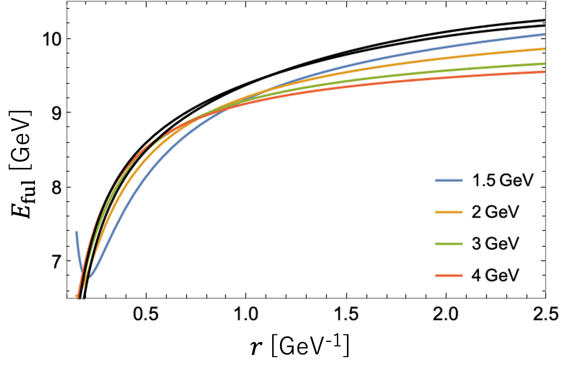
Figure 5: Comparison of $V_{\rm QCD}^{\rm MNA}+V_{\rm NA}$ in the FTRS method (black lines) and $E_{\text{full}}$ in the fixed-order perturbative series (colored lines) as functions of $r$. An arbitrary $r$-independent constant is added to the former. The latter lines are for $\mu=4,3,2,1.5$ GeV from left to right. In the former potential $\log(\mu_{\rm US}r)+\gamma_{E}$ is set to one or zero and the result changes only slightly. In the latter $\mu_{\rm US}$ is set to 1 GeV.

We choose $(a,u^{\prime})=(1,-1/2)$ for $V_{\rm QCD}^{\rm MNA}$ and $(a,u^{\prime})=(1,-1)$ for $V_{\rm NA}$ such that the renormalons of the individual potentials are suppressed minimally. (These correspond to the ordinary Fourier transformation of both potentials.) We add an $r$-independent constant to the FTRS result to facilitate the comparison. For estimating the US effects, $\log(\mu_{\rm US}r)+\gamma_{E}$ is set to one or zero before the Fourier transform, by which $V_{\rm QCD}^{\rm MNA}+V_{\rm NA}$ changes the shape only slightly in the displayed range. We see that, at short distances, the FTRS result reproduces well the shape of $E_{\rm full}$ for a larger $\mu$, while at larger distances it reproduces the shape of $E_{\rm full}$ for a smaller $\mu$. In general, the convergence of the potentials are better at smaller $r$ both for the FTRS and fixed-order calculations, and $r\Lambda_{\overline{\rm MS}}$ would be reasonably smaller than unity in the displayed range. Hence, we observe a plausible feature in this comparison.

We have also examined $V_{\rm QCD}^{\rm MNA}+V_{\rm NA}$ in the DSRS method. At $r\lesssim 0.2~{}{\rm GeV}^{-1}$, the DSRS result agrees well with the FTRS result, while at larger distances it deviates from the FTRS result (and also from the fixed-order result). In view of the analysis in Sec. 2 this indicates that the convergence of the DSRS result is quite slow compared to the FTRS result.

5 Summary and Conclusion

In Sec. 2 we have seen that in the LL approximation of the FTRS method $V_{\rm NA}(r)$ includes the ${\cal O}(\Lambda_{\rm QCD}^{2}/m)$ renormalon. In Sec. 3 we have seen that the fixed-order perturbative series of the total energy of the quarkonium system improves stability against scale variation and convergence as we incorporate possible cancellation of the ${\cal O}(\Lambda_{\rm QCD})$ and ${\cal O}(\Lambda_{\rm QCD}^{2}/m)$ renormalons successively. In Sec. 4 we have seen that the FTRS and DSRS estimates of the ${\cal O}(\Lambda_{\rm QCD}^{2}/m)$ renormalons of $V_{\mathrm{NA}}$ and $2\,m_{\rm pole}^{\rm MNA}$ from the known first two terms do not show a sign of convergence, while there is a tendency of partial cancellation between them. On the other hand, the FTRS estimate of the PV part of $V_{\rm QCD}^{\rm MNA}(r)+V_{\rm NA}(r)$ shows a reasonable agreement with the fixed-order total energy at $r<2.5~{}{\rm GeV}^{-1}$.

These analysis results are mutually consistent and also consistent with the hypothesis that both $2m_{\rm pole}$ and $V_{1/r^{2}}$ include the ${\cal O}(\Lambda_{\rm QCD}^{2}/m)$ renormalons and that they cancel each other. Since there is no argument which forbids existence of the ${\cal O}(\Lambda_{\rm QCD}^{2}/m)$ renormalons, we interpret our analysis results to be positive indications for their existence and cancellation.

The analysis in Sec. 3 indicates that already in the current status there is a possibility to improve the accuracy of the theoretical prediction for the quarkonium energy by incorporating cancellation of the ${\cal O}(\Lambda_{\rm QCD}^{2}/m)$ renormalons. Note that the current calculations of the heavy quarkonium spectrum do not incorporate this cancellation mechanism due to the use of the $\epsilon$ expansion [20]. A proper account of this cancellation may improve accuracy of the charm and bottom quark mass determinations from the charmonium and bottomonium $1S$ energy levels [21, 22], for instance.

References

- [1] A. Pineda, Ph.D. Thesis (1998).
- [2] A. H. Hoang, M. C. Smith, T. Stelzer and S. Willenbrock, Phys. Rev. D 59, 114014 (1999) [arXiv:hep-ph/9804227 [hep-ph]].
- [3] M. Beneke, Phys. Lett. B 434, 115-125 (1998) [arXiv:hep-ph/9804241 [hep-ph]].
- [4] M. Neubert, Phys. Lett. B 393 (1997), 110-118 doi:10.1016/S0370-2693(96)01600-0 [arXiv:hep-ph/9610471 [hep-ph]].
- [5] N. Brambilla, A. Pineda, J. Soto and A. Vairo, Phys. Rev. D 60 (1999), 091502 doi:10.1103/PhysRevD.60.091502 [arXiv:hep-ph/9903355 [hep-ph]].
- [6] Y. Sumino and H. Takaura, JHEP 05 (2020), 116 doi:10.1007/JHEP05(2020)116 [arXiv:2001.00770 [hep-ph]].
- [7] S. Recksiegel and Y. Sumino, Phys. Rev. D 67 (2003), 014004 doi:10.1103/PhysRevD.67.014004 [arXiv:hep-ph/0207005 [hep-ph]].
- [8] M. Beneke and V. M. Braun, Phys. Lett. B 348 (1995), 513-520 doi:10.1016/0370-2693(95)00184-M [arXiv:hep-ph/9411229 [hep-ph]].
- [9] Y. Hayashi, Y. Sumino and H. Takaura, Phys. Lett. B 819 (2021), 136414 doi:10.1016/j.physletb.2021.136414 [arXiv:2012.15670 [hep-ph]].
- [10] Y. Hayashi, Y. Sumino and H. Takaura, JHEP 02 (2022), 016 doi:10.1007/JHEP02(2022)016 [arXiv:2106.03687 [hep-ph]].
- [11] Y. Hayashi, G. Mishima, Y. Sumino and H. Takaura, JHEP 06 (2023), 042 doi:10.1007/JHEP06(2023)042 [arXiv:2303.16392 [hep-ph]].
- [12] B. A. Kniehl, A. A. Penin, M. Steinhauser and V. A. Smirnov, Phys. Rev. D 65 (2002), 091503 doi:10.1103/PhysRevD.65.091503 [arXiv:hep-ph/0106135 [hep-ph]].
- [13] N. Brambilla, A. Pineda, J. Soto and A. Vairo, Rev. Mod. Phys. 77 (2005), 1423 doi:10.1103/RevModPhys.77.1423 [arXiv:hep-ph/0410047 [hep-ph]].
- [14] N. Brambilla, A. Pineda, J. Soto and A. Vairo, Phys. Lett. B 470 (1999), 215 doi:10.1016/S0370-2693(99)01301-5 [arXiv:hep-ph/9910238 [hep-ph]].
- [15] B. A. Kniehl and A. A. Penin, Nucl. Phys. B 563 (1999), 200-210 doi:10.1016/S0550-3213(99)00564-7 [arXiv:hep-ph/9907489 [hep-ph]].
- [16] Y. Sumino, [arXiv:1411.7853 [hep-ph]].
- [17] Y. Sumino, Phys. Lett. B 571 (2003), 173-183 doi:10.1016/j.physletb.2003.05.010 [arXiv:hep-ph/0303120 [hep-ph]].
- [18] K. Melnikov and T. v. Ritbergen, Phys. Lett. B 482 (2000), 99-108 doi:10.1016/S0370-2693(00)00507-4 [arXiv:hep-ph/9912391 [hep-ph]].
- [19] Y. Schroder, Phys. Lett. B 447 (1999), 321-326 doi:10.1016/S0370-2693(99)00010-6 [arXiv:hep-ph/9812205 [hep-ph]].
- [20] A. H. Hoang, Z. Ligeti and A. V. Manohar, Phys. Rev. Lett. 82 (1999), 277-280 doi:10.1103/PhysRevLett.82.277 [arXiv:hep-ph/9809423 [hep-ph]].
- [21] Y. Kiyo, G. Mishima and Y. Sumino, Phys. Lett. B 752 (2016), 122-127 [erratum: Phys. Lett. B 772 (2017), 878-878] doi:10.1016/j.physletb.2015.11.040 [arXiv:1510.07072 [hep-ph]].
- [22] C. Peset, A. Pineda and J. Segovia, JHEP 09 (2018), 167 doi:10.1007/JHEP09(2018)167 [arXiv:1806.05197 [hep-ph]].