The Quantum Echo in Two-component Bose-Einstein Condensate

Abstract

The development of ultracold atom technology has enabled the precise investigations into quantum dynamics of quantum gases. Recently, inspired by experimental advancement, the $SU(1,1)$ echo, akin to the well-known $SU(2)$ spin echo, has been proposed for single-component Bose-Einstein condensate (BEC). In this paper, we investigate the possibility of quantum echo in the more intricate two-component BEC using the non-compact Lie group $Sp(4,R)$, which describes the quantum dynamics of such systems. We demonstrate that quantum echo can occur for the fully condensed state, as well as any $Sp(4,R)$ coherent state by applying a driving protocol consisting of two steps in each period. The first step can be any Bogoliubov Hamiltonian, while the second step is a Hamiltonian with all interactions turned off, which plays a similar role as the $\pi$-pulse in spin echo. We confirm our theoretical results with numerical calculations for different examples of two-component BEC. We further consider the effect of interactions between the excited boson modes on the quantum echo process and discuss the possible experiment implementation of this quantum echo.

I Introduction

In the past decades, ultracold-atomic systems have emerged as a powerful tool for the precise exploration of dynamics within quantum systems, as they offer high controllability and tunability [1, 2, 3]. Recently, The Chicago group’s experiments on Bose-Einstein condensates (BECs) have unveiled phenomena like Bose fireworks and quantum revival of BEC [4, 5, 6, 7, 8, 9, 10, 11, 12]. The latter phenomenon inspired the study of quantum echo, i.e. the revival of the quantum state of a system after applying a specific driving protocol, using the $SU(1,1)$ group in single-component BEC [13, 14, 15, 16], which resembles the $SU(2)$ spin echo [17].

The two-component BEC, comprising two species or internal states of bosonic atoms, presents a more intricate system. The two-component BEC has been realized in various ultracold atom systems [18, 19, 20, 21, 22, 23, 24, 25, 26, 27, 28, 29], and received extensive investigations [30, 31, 32, 33, 34, 35, 36, 37, 38, 39, 40, 41, 42, 43, 44]. Given the tunability of the interaction between different species of atoms through Feshbach resonances [23], one may wonder whether such a quantum echo can occur in this more complicated two-component BEC system.

In this paper, we address this problem by using the general formalism presented in Ref.[45], which employs the so-called real symplectic group $Sp(4,R)$ to deal with the quantum dynamics of the two-component BEC. The $Sp(4,R)$ group, a non-compact Lie group, preserves the canonical commutation relations of boson operators [46] and finds applications across various areas of physics, such as quantum information [47, 48, 49], high energy physics [50, 51, 52, 53], and cold atoms [54, 55, 56, 45]. In Ref.[45], by mapping the time evolution operator to an $Sp(4,R)$ matrix, it is revealed that the ground state of two-component BEC will evolve to an $Sp(4,R)$ coherent state under the effective interaction between atoms, and any coherent state will evolve to another coherent state. These coherent states can be parameterized by a six-dimensional manifold $Sp(4,R)/U(2)$, i.e. the quotient space of $Sp(4,R)$ and the unitary group of order two $U(2)$. Thus, the time evolution will correspond to a trajectory in this manifold.

Utilizing this formalism, we show that through a two-step periodic driving protocol, the ground state or any $Sp(4,R)$ coherent state of a two-component BEC can revert to its original form after two driving periods. The first-step Hamiltonian, $\hat{H}_{1}$, can be any Bogoliubov Hamiltonian, while in the second step, $\hat{H}_{2}$, the interactions are turned off. We provide a methodology to calculate $\hat{H}_{2}$ from $\hat{H}_{1}$. This is demonstrated through two examples: a time-independent $\hat{H}_{1}$ and a time-dependent $\hat{H}_{1}$, with numerical results corroborating our theory. We also examine the quantum echo breaking effect due to interactions between excited boson modes and analyze how this effect varies with the kinetic to interaction strength ratio in the first-step Hamiltonian. The paper concludes with a discussion on potential implementations of these novel quantum echoes in cold atom experiments.

This paper is organized as follows: in Sec. II, we review the formalism using $Sp(4,R)$ group to deal with the quantum dynamics of two-component BEC; in Sec. III, we prove the two-step driving protocol can make the quantum echo happen; in Sec. IV, we apply this driving protocol to two different examples, and present the numerical results to confirm our proof; in Sec. V, we consider the interaction effect.

II The quantum dynamics and $Sp(4,R)$ symmetry

We consider the physical process that a two-component Bose gas is prepared in a fully condensed state, i.e. all particles condensed in the zero momentum modes, then the system evolves under the Bogoliubov Hamiltonian. The general form of this quench Bogoliubov Hamiltonian can be written as $\hat{H}_{\mathrm{Bg}}(t)=\sum_{\mathbf{k}\neq\mathbf{0}}\hat{H}_{\mathbf{k}}(t)+\mathrm{const.}$, where

$$\hat{H}_{\mathbf{k}}(t)=\hat{\Psi}_{\mathbf{k}}^{\dagger}\mathcal{H}_{\mathbf{k}}(t)\hat{\Psi}_{\mathbf{k}},\ \mathcal{H}_{\mathbf{k}}(t)=\left(\begin{array}[]{cc}\xi_{\mathbf{k}}(t)&\eta(t)\\ \eta^{*}(t)&\xi_{\mathbf{k}}^{*}(t)\end{array}\right),$$ (3)

with $\hat{\Psi}_{\mathbf{k}}=(a_{1,\mathbf{k}},a_{2,\mathbf{k}},a_{1,-\mathbf{k}}^{\dagger},a_{2,-\mathbf{k}}^{\dagger})^{T}$ [57, 45]. Here $\xi_{\mathbf{k}}(t)$ is a $2\times 2$ Hermitian matrix given by $\xi_{\mathbf{k},ij}(t)=\frac{1}{2}[\varepsilon_{\mathbf{k},ij}(t)+g_{ij}(t)\psi_{i}\psi_{j}^{*}]$, and $\eta(t)$ is a complex symmetric matrix given by $\eta_{ij}(t)=\frac{1}{2}g_{ij}(t)\psi_{i}\psi_{j}$, and $i,j=1,2$ label the two species of bosons. The diagonal elements of $\varepsilon_{\mathbf{k}}(t)$ are the kinetic terms, whereas the off-diagonal elements are the spin-orbit coupling terms. $g_{ij}(t)$ represent the intra- and inter-species interaction strengths of these two species of bosons. $\psi_{i}=\sqrt{N_{i}/V}e^{i\theta}$ are the condensate wavefunctions of the zero momentum modes. And for simplicity, we set $\hbar=1$.

On the other hand, the two species of the boson operators naturally give a representation of the Lie algebra of the real symplectic group $Sp(4,R)$ [46, 58]. The generators of this Lie algebra can be defined as

$$\hat{\mathcal{X}}_{ij}=a_{i,\mathbf{k}}a_{j,-\mathbf{k}}+a_{j,\mathbf{k}}a_{i,-\mathbf{k}},$$

$$\hat{\mathcal{X}}^{ij}=a_{i,\mathbf{k}}^{\dagger}a_{j,-\mathbf{k}}^{\dagger}+a_{j,\mathbf{k}}^{\dagger}a_{i,-\mathbf{k}}^{\dagger},$$

$$\hat{\mathcal{X}}_{l}^{k}=a_{k,\mathbf{k}}^{\dagger}a_{l,\mathbf{k}}+a_{l,-\mathbf{k}}a_{k,-\mathbf{k}}^{\dagger},$$ (4)

where $i,j,k,l=\{1,2\}$, and ten of them are independent. It can be verified that the above operators satisfy the $\mathfrak{sp}(4,R)$ Lie algebra commutation relation. These operators have a one-to-one correspondence with the matrix representation of the $\mathfrak{sp}(4,R)$ Lie algebra. This correspondence can be revealed by rewriting the operators defined in Eq.(II) as

$$\hat{\mathcal{X}}_{ij}=\hat{\Psi}_{\mathbf{k}}^{\dagger}\kappa Y_{ij}\hat{\Psi}_{\mathbf{k}},\ \hat{\mathcal{X}}^{ij}=\hat{\Psi}_{\mathbf{k}}^{\dagger}\kappa Y^{ij}\hat{\Psi}_{\mathbf{k}},\ \hat{\mathcal{X}}_{l}^{k}=\hat{\Psi}_{\mathbf{k}}^{\dagger}\kappa Y_{l}^{k}\hat{\Psi}_{\mathbf{k}},$$ (5)

where $\kappa=\mathrm{diag}(1,1,-1,-1)$ [58, 45]. Here, these $4\times 4$ matrices $\{Y_{ij},Y^{ij},Y_{l}^{k}\}$ are the matrix representation of the Lie algebra $\mathfrak{sp}(4,R)$, and their explicit form is given in Appendix A. Then, we can write the Bogoliubov Hamiltonian $\hat{H}_{\mathbf{k}}$ in terms of these generators as

$$\hat{H}_{\mathbf{k}}(t)=\xi_{\mathbf{k},ij}(t)\hat{\mathcal{X}}_{j}^{i}+\frac{1}{2}\eta_{ij}(t)\hat{\mathcal{X}}_{ij}+\frac{1}{2}\eta_{ij}^{*}(t)\hat{\mathcal{X}}^{ij},$$ (6)

where we have adopted the Einstein summation convention, i.e. the repeated indices $i$ and $j$ are summed over. In the following, we always adopt this convention implicitly. Hence, the time evolution operator

$$\hat{U}_{\mathbf{k}}(t)=\mathcal{T}e^{-i\int_{0}^{t}\hat{H}_{\mathbf{k}}(t^{\prime})dt^{\prime}}$$ (7)

gives a representation of the real symplectic group $Sp(4,R)$, i.e. $\hat{U}_{\mathbf{k}}(t)$ has a one-to-one correspondence to a matrix in the group $Sp(4,R)$, which is given by

$$U_{\mathbf{k}}(t)=\mathcal{T}e^{-i\int_{0}^{t}\kappa\mathcal{H}_{\mathbf{k}}(t^{\prime})dt^{\prime}}.$$ (8)

Here, $\mathcal{T}$ is the time ordering operator. This can be seen by noticing that the matrix corresponding to the operator $\hat{H}_{\mathbf{k}}(t)$ is

$$\kappa\mathcal{H}_{\mathbf{k}}(t)=\xi_{\mathbf{k},ij}(t)Y_{j}^{i}+\frac{1}{2}\eta_{ij}(t)Y_{ij}+\frac{1}{2}\eta_{ij}^{*}(t)Y^{ij}.$$

Since the matrix $U_{\mathbf{k}}(t)$ is a real symplectic matrix, it has the form [46]

$$U_{\mathbf{k}}(t)=\left(\begin{array}[]{cc}\mathcal{U}(t)&\mathcal{V}(t)\\ \mathcal{V}(t)^{*}&\mathcal{U}(t)^{*}\end{array}\right),$$ (11)

where $\mathcal{U}(t),\mathcal{V}(t)$ are $2\times 2$ matrices satisfying

$$\mathcal{U}(t)\mathcal{U}(t)^{\dagger}-\mathcal{V}(t)\mathcal{V}(t)^{\dagger}=I,\ \mathcal{U}(t)\mathcal{V}(t)^{T}=\mathcal{V}(t)\mathcal{U}(t)^{T}.$$ (12)

In order to calculate the time evolution of the fully condensed state, one can decompose $\hat{U}_{\mathbf{k}}(t)$ as

$$\hat{U}_{\mathbf{k}}(t)=e^{-\frac{1}{2}Z_{ij}(t)\hat{\mathcal{X}}^{ij}}e^{\zeta_{kl}(t)\hat{\mathcal{X}}_{l}^{k}}e^{-\frac{1}{2}\nu_{ij}(t)\hat{\mathcal{X}}_{ij}},$$ (13)

which is called normal order decomposition [46, 45]. With this decomposition, the fully condensed state $|\mathbf{0}\rangle$ evolves as

$$\hat{U}_{\mathbf{k}}(t)|\mathbf{0}\rangle=\mathcal{N_{\mathbf{k}}}e^{-\frac{1}{2}Z_{ij}(t)\hat{\mathcal{X}}^{ij}}|\mathbf{0}\rangle\equiv|Z(t)\rangle,$$ (14)

where $|Z(t)\rangle$ is an $Sp(4,R)$ coherent state and $\mathcal{N_{\mathbf{k}}}$ is normalization factor. At any time $t$ of the evolution, $Z(t)$ is [59, 45]

$$Z(t) = \mathcal{V}(t)[\mathcal{U}(t)^{*}]^{-1},$$ (15)

where $\mathcal{U}(t),\mathcal{V}(t)$ is defined in Eq.(11). By using the Eq.(12), it can be shown that at any time t, $Z(t)$ is a $2\times 2$ symmetric complex matrix, and $I-Z(t)^{\dagger}Z(t)$ is positive definite, where $I$ is $2\times 2$ identity matrix. Mathematically, $Z(t)$ lies in a six-dimensional manifold called Cartan classical domain, and is isomorphic to the quotient space $Sp(4,R)/U(2)$ [60, 46], where $U(2)$ is the unitary group of degree 2. Thus, $Z(t)$ gives a trajectory in this six-dimensional manifold. And if the initial state is arbitrary coherent state $|Z_{0}\rangle$, the time evolution of this coherent is also a coherent state, i.e. $\hat{U}_{\mathbf{k}}(t)|Z_{0}\rangle=|Z^{\prime}(t)\rangle$, and $Z^{\prime}(t)$ is given by [45, 59]

$$Z^{\prime}(t)=[\mathcal{U}(t)Z_{0}+\mathcal{V}(t)][\mathcal{V}(t)^{*}Z_{0}+\mathcal{U}(t)^{*}]^{-1}.$$ (16)

With this general formalism dealing with the time evolution of two-component BEC in hand, we are ready to study the quantum echo of the two-component BEC system.

III The quantum echo

In this section, we will study the problem of quantum echo for boson modes in generic $\pm\mathbf{k}\neq\mathbf{0}$ momenta by considering a periodic driving protocol similar to Ref.[13, 15]. In this driving protocol, each period consists of two steps: in the first step, the Hamiltonian $\hat{H}_{1}$ is a generic two-component Bogoliubov Hamiltonian defined in Eq.(6); in the second step, the Hamiltonian $\hat{H}_{2}$ only includes these $\hat{\mathcal{X}}_{j}^{i}$ operators, i.e. turning off all the intra- and inter-species interaction strengths. We will show how to obtain the explicit form of the second-step Hamiltonian $\hat{H}_{2}$ that make the initial state, either $|\mathbf{0}\rangle$ or a generic coherent state $|Z_{0}\rangle$, reverse to itself after two period of driving for any given Bogoliubov Hamiltonian $\hat{H}_{1}$.

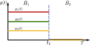
Figure 1: Schematics for the driving protocol. In the first step of a period, the Hamiltonian can be any Bogoliubov Hamiltonian. However, in the second step of a period, the all the interaction strengths should be turned off.

In the $m$th period, when $(m-1)T<0\leq(m-1)T+t_{1}$, the Hamiltonian is

$$\hat{H}_{1} = \xi_{ij}(t)\hat{\mathcal{X}}_{j}^{i}+\frac{1}{2}\eta_{ij}(t)\hat{\mathcal{X}}_{ij}+\frac{1}{2}\eta_{ij}^{*}(t)\hat{\mathcal{X}}^{ij},$$ (17)

and when $(m-1)T+t_{1}<t\leq mT$

$$\hat{H}_{2} = \frac{1}{2}\varepsilon_{ij}\hat{\mathcal{X}}_{j}^{i},$$ (18)

where $T=t_{1}+t_{2}$ is the duration of each period. Here we have omitted the subscript $\mathbf{k}$ for simplicity. Thus, for such a quantum echo to happen, we require that the time evolution operators $\hat{U}_{1}(t_{1})$ and $\hat{U}_{2}(t_{2})$ of these two steps acting on any coherent state $|Z_{0}\rangle$ gives

$$(\hat{U}_{2}(t_{2})\hat{U}_{1}(t_{1}))^{2}|Z_{0}\rangle=|Z_{0}\rangle.$$ (19)

According to Eq.(16), this condition is equivalent to

$$U(T)^{2}=(U_{2}(t_{2})U_{1}(t_{1}))^{2}=\pm 1,$$ (20)

where $U_{i}(t_{i}),i=1,2$ are the time evolution matrix corresponding to $\hat{U_{i}}(t_{i})$. Next we will focus the case $U(T)^{2}=-1$, since the result for $U(T)^{2}=1$ case can be obtained by redefined $U(T)^{2}$ from $U(T)^{2}=-1$ case as $U(T)$.

Since $U(T)$ is also a real symplectic matrix i.e. having the form of Eq.(11), substituting its elements $\mathcal{U},\mathcal{V}$ into Eq.(20) leads to

$$\mathcal{U}^{2}+\mathcal{V}\mathcal{V}^{*} = \mathcal{U}^{*2}+\mathcal{V}^{*}\mathcal{V}=-1,$$

$$\mathcal{U}\mathcal{V}+\mathcal{V}\mathcal{U}^{*} = 0.$$ (21)

By using the property of real symplectic matrix $\mathcal{U}\mathcal{U}^{\dagger}-\mathcal{V}\mathcal{V}^{\dagger}=I,\ \mathcal{U}\mathcal{V}^{T}=\mathcal{V}\mathcal{U}^{T}$, the Eqs.(III) result in

$$\mathcal{U}=-\mathcal{U}^{\dagger}.$$ (22)

This is the condition that $U(T)$ should satisfy for the quantum echo to happen.

Next, we will construct an explicit form of $U(T)$. We recall that for the $SU(1,1)$ case, an $SU(1,1)$ matrix satisfying $U^{2}=-1$ can be given by

$$(e^{i\pi\frac{\sigma_{z}}{2}}e^{i(\alpha_{+}\sigma^{+}-\alpha_{-}\sigma^{-})})^{2}=-1,$$ (23)

where $\{\sigma_{z}/2,\sigma^{+},-\sigma^{-}\}$ are the generators of $SU(1,1)$ group, with $\sigma_{x,y,x}$ the Pauli matrices and $\sigma^{\pm}=1/2(\sigma_{x}\pm i\sigma_{y})$, and $\alpha_{\pm}$ are arbitrary complex numbers. We notice the resemblance in form between $\{\sigma_{z},\sigma^{+},-\sigma^{-}\}$ and $\{Y_{l}^{k},Y_{ij},Y^{ij}\}$. Inspired by this resemblance, we expect that for the $Sp(4,R)$ case, the matrix $U(T)$ satisfying $U(T)^{2}=-1$ is given by

$$U(T) = e^{i\frac{\pi}{2}(Y_{1}^{1}+Y_{2}^{2})}e^{\frac{i}{2}(\eta_{ij}Y^{ij}+\eta_{ij}^{*}Y_{ij})}$$ (24)

where $\eta$ is a $2\times 2$ symmetric complex matrix. Since $e^{i\frac{\pi}{2}(Y_{1}^{1}+Y_{2}^{2})}=\mathrm{diag}(i,i,-i,-i)$, substituting the above equation to Eq.(22) leads to that the sub-matrix $\mathcal{U}_{0}$ of $U_{0}=e^{\frac{i}{2}(\eta_{ij}Y^{ij}+\eta_{ij}^{*}Y_{ij})}$ is Hermitian, i.e. $\mathcal{U}_{0}=\mathcal{U}_{0}^{\dagger}$. In Appendix A, we give the explicit expression of $\mathcal{U}_{0}$ and also prove that $\mathcal{U}_{0}$ is Hermitian. As a result, we prove that the form of $U(T)$ given in Eq.(24) actually satisfy $U(T)^{2}=-1$.

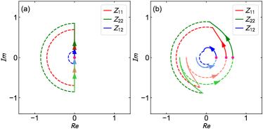
Figure 2: Trajectories of the elements of $Z(t)$ when $\eta_{11}=1,\eta_{22}=3/2,\eta_{12}=1/2$ for (a) the initial state is $|\mathbf{0}\rangle$, and (b) the initial state is a coherent state $|Z_{0}\rangle$ with $Z_{0}=\left(\begin{array}[]{cc}1/2&1/4\\ 1/4&2/3\end{array}\right)$. The evolution includes two periods. The lines (both solid and dashed) with darker colors represent the first period, and the line with lighter colors represent the second period. The solid lines represent the first steps and the dashed lines represent the second steps.

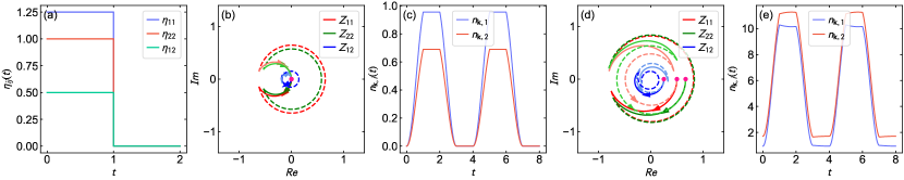
Figure 3: Quantum echo when the interaction strengths are all constant in the first step of each period. (a) The interaction terms $\eta_{ij}(t)$ in one period. (b) The trajectory of the $Z(t)$ matrix in the parameter space when initial state is $|\mathbf{0}\rangle$. The purple dot represents the initial state, the arrows represent the direction of the trajectories as time evolves. The solid lines represent the first step and the dashed lines represent the second step. The lines with deep colors are the first period and light-colored ones represent the second period. (c) The time evolution of the particle number for each species of bosons when initial state is a vacuum. (d), (e) the same Hamiltonian as (c) and (d) but the initial is a generic coherent state $|Z_{0}\rangle$ which is the same as the one in Figure 2.

With the general form of $U(T)$, we can find the $\hat{H}_{2}$ that make the quantum echo happen for arbitrary $\hat{H}_{1}$. Since $\hat{H}_{1}$ is of the general form of Eq.(6), its corresponding time evolution matrix is also of the general form of real symplectic matrix Eq.(11), i.e.

$$U_{1}(t_{1})=\left(\begin{array}[]{cc}\mathcal{U}_{1}(t_{1})&\mathcal{V}_{1}(t_{1})\\ \mathcal{V}_{1}(t_{1})^{*}&\mathcal{U}_{1}(t_{1})^{*}\end{array}\right).$$ (27)

However, $\hat{H}_{2}$ only has $\hat{\mathcal{X}}_{j}^{i}$ terms, thus, its corresponding time evolution matrix is block diagonal, i.e.

$$U_{2}(t_{2})=\left(\begin{array}[]{cc}\mathcal{U}_{2}(t_{2})&0\\ 0&\mathcal{U}_{2}(t_{2})^{*}\end{array}\right).$$ (30)

And the constraints on the real symplectic matrix Eq.(12) also results in that $\mathcal{U}_{2}(t_{2})$ is unitary. Then, by substituting the elements of $U_{1}(t_{1})$ and $U_{2}(t_{2})$ into $U(T)=U_{2}(t_{2})U_{1}(t_{1})$, we have

$$-i\mathcal{U}_{1}(t_{1})=\mathcal{U}_{2}(t_{2})^{-1}\mathcal{U}_{0}.$$ (31)

Since we have shown that $\mathcal{U}_{2}(t_{2})^{-1}$ is unitary and $\mathcal{U}_{0}$ is Hermitian, the right-hand side of the above equation is just the polar decomposition of $-i\mathcal{U}_{1}(t_{1})$. The polar decomposition of a complex matrix is the factorization of this matrix into a product of unitary matrix and a Hermitian matrix. And the polar decomposition of a square matrix always exist. Hence, by doing the polar decomposition we can find $\mathcal{U}_{2}(t_{2})$. And the explicit form of $\mathcal{H}_{2}$ is given by

$$\mathcal{H}_{2}=\kappa\ln(\mathcal{U}_{2}(t_{2}))/(-it_{2}),$$ (32)

where $\kappa=\mathrm{diag}(1,1,-1,-1)$.

To have a better understanding of why we choose $U(T)$ to have the form of Eq.(24), we can let $\hat{H}_{1}=-\frac{1}{2}(\eta_{ij}\hat{\mathcal{X}}^{ij}+\eta_{ij}^{*}\hat{\mathcal{X}}_{ij})$, $\hat{H}_{2}=-\frac{\pi}{2}(\hat{\mathcal{X}}_{1}^{1}+\hat{\mathcal{X}}_{2}^{2})$, and the times $t_{1}=t_{2}=1$. Figure (2) shows the trajectory of the elements of the matrix $Z_{t}$ in the complex plane for the cases when the initial state is $|\mathbf{0}\rangle$ and a generic coherent state $|Z_{0}\rangle$ respectively. It can be seen that in both cases, all the trajectories perfectly return to their initial points, which confirms above proof. From this figure, we can see that for both cases, the second step $\hat{H}_{2}$ amounts to a $\pi$ rotation for all the elements of the $Z_{t}$ matrix. It reverses the direction of the trajectories and make the trajectories return to its initial points. Thus, we can see that the second-step Hamiltonian plays a similar role to the $\pi$ pulse in the $SU(2)$ spin echo. Meanwhile, when the initial state is $|\mathbf{0}\rangle$, the second step in the second period is not necessary for quantum echo, and applying $\hat{H}_{1},\hat{H}_{2}$ and $\hat{H}_{1}$ in consequence suffices to make the state return to its initial state. However, if the initial state is a generic coherent state, the full driven protocol is necessary for the quantum echo to happen.

IV Numerical results

In last section, we have provided a protocol that can bring any coherent state back to itself after two periods of driving for any Bogoliubov Hamiltonian $\hat{H}_{1}$. Briefly, In this protocol, each period consists two steps: the first step can be any Bogoliubov Hamiltonian $\hat{H}_{1}$, and the second step is a quadratic Hamiltonian $\hat{H}_{2}$ with all interaction strengths turned off. The Hamiltonian in the second step can be found by doing a polar decomposition for the $2\times 2$ sub-matrix of the time evolution matrix $U_{1}(t_{1})$ as shown in Eq.(31) and Eq.(32).

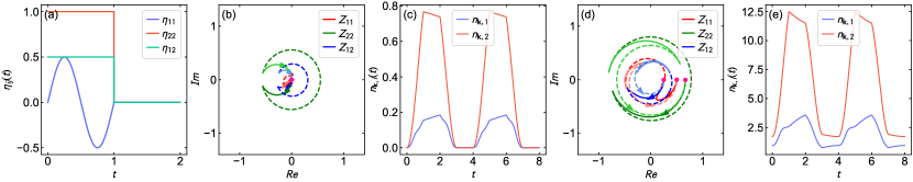
Figure 4: Quantum echo when one interaction strength is a sine wave. (a) The interactions $g_{ij}(t)$ in a period. (b) The trajectory of the $Z(t)$ matrix in the parameter space when initial state is the vacuum. The convention in this figure is the same as Figure 3. (c) The time evolution of the particle number of each species of bosons when initial state is a vacuum. (d), (e) the same Hamiltonian as (c) and (d) but the initial is a generic coherent state $|Z_{0}\rangle$, which is the one we used in Figure 2.

In this section, we will apply this protocol to some examples and present the numerical results. The first example is the case when the interaction strengths all keep constant in the first step of a period as shown in Figure 3. For simplicity, in the first step of each driving period, we set the masses of the two species of bosons equal and set the spin-orbit coupling as 0, more specifically we set $\varepsilon_{\mathbf{k}}=\mathrm{diag}(1,1)$, where the matrix $\varepsilon_{\mathbf{k}}$ is defined in the Eq.(3). And the interaction terms $\eta_{ij}$ are chosen as $\eta_{11}=1.25,\ \eta_{22}=1,\ \eta_{12}=0.5$ as shown in Figure 3(a). And we choose the duration of each step equal i.e. $t_{1}=t_{2}=1$. According to Eq.(31) and Eq.(32), the Hamiltonian in the second step is

$$\mathcal{H}_{2}=\left(\begin{array}[]{cc}\varepsilon&0\\ 0&\varepsilon^{*}\end{array}\right),\ \varepsilon\simeq-\left(\begin{array}[]{cc}2.85&0.21\\ 0.21&2.75\end{array}\right).$$ (37)

Here, we can see that with the interaction strengths turned off, only the kinetic terms and the spin-orbit coupling terms left in $\mathcal{H}_{2}$. However, the diagonal terms in $\varepsilon$ are no longer equal, which means different chemical potentials for these two species of bosons are required. Meanwhile, the off-diagonal terms are also no longer $0$, requiring non-zero spin-orbit coupling.

The numerical results for this case are shown in Figure 3. Figure 3(a) shows the values of the interaction strengths. Figure 3(b) shows the evolution of the three independent complex elements of the matrix $Z(t)$ in the complex plane when the initial state is the fully condensed state $|\mathbf{0}\rangle$. In Figure 3(c), we show the evolution of the particle number of each component of boson, which can be calculated using the method presented in Ref.[45]. Figure 3(d) and (e) show the trajectories and particle numbers when the initial state is a generic non-vacuum coherent state.

The second example is the case when one of the interaction strengths is a sine wave in the first step of each period as shown in Figure 4. Here, we still choose the $\varepsilon_{\mathbf{k}}$ matrix in the first-step Hamiltonian as diagonal, i.e. $\varepsilon(\mathbf{k})=\mathrm{diag}(1,1)$, and set the duration of each step equal i.e. $t_{1}=t_{2}=1$. For the interaction terms, $\eta_{11}=1/2\sin(2\pi t),\ \eta_{22}=1$ and $\eta_{12}=0.5$, as shown in Figure 4. Using the same procedure, we can calculate the second-step Hamiltonian $\mathcal{H}_{2}=\mathrm{diag}(\varepsilon,\varepsilon^{*})$, where

$$\varepsilon\simeq-\left(\begin{array}[]{cc}2.02&0.36-0.009i\\ 0.36+0.009i&2.73\end{array}\right).$$ (40)

In Figure 4, we show the evolution trajectories in the parameter space and the evolution of particle numbers when the initial state is a fully condensed state and a generic coherent state.

From the numerical results present in Figure 3 and 4, we can see that our formalism can clearly display how the initial state evolves in the whole driving process. And it is clearly shown that for these two examples, the driving protocol can bring both the fully condensed state and a generic state back to themselves after two periods. Meanwhile, in these examples, the trajectories of the case with a generic coherent state as the initial state are more complicated than the case with a fully condensed state as initial state. Furthermore, we also show the time evolution of the particle numbers of the two species of bosons. The particle numbers increase rapidly in the first step of the first period, and then in the second step they cease to grow. In the first step of the second period, the particle numbers start to decrease. Finally, they return to their initial values. Thus, numerical results clearly demonstrate how the quantum echo happens in the two-component BEC systems.

V Interaction effect

In this section, we will consider the interaction effect in the quantum echo process. Similar to the one component BEC [15], the interaction between these boson modes in two-component BEC can be given as $\hat{V}=\sum_{i,j}(4\hat{n}_{i,\mathbf{k}}\hat{n}_{j,-\mathbf{k}}+\hat{n}_{i,\mathbf{k}}\hat{n}_{j,\mathbf{k}}+\hat{n}_{i,-\mathbf{k}}\hat{n}_{j,-\mathbf{k}})$. When there are a large amount of boson modes excited in the $\pm\mathbf{k}$ momenta, the interaction between these excitations cannot be ignored. As a result, the quantum echo process will be broken. By calculating the particle numbers in the end of $2m$th period, we want to reveal the interplay of the interactions between boson modes and the parameters in the original first-step Hamiltonian $\hat{H}_{1}$ in this quantum echo breaking process.

For simplicity, we consider the following two-step driving

$$\hat{H}_{1}^{\prime} = \hat{H}_{1}+\tilde{g}\hat{V},$$

$$\hat{H}_{2} = \frac{1}{2}\varepsilon_{ij}\hat{\mathcal{X}}_{j}^{i},$$ (41)

where $\hat{H}_{1}=(E\delta_{ij}+\gamma\eta_{ij})(\hat{\mathcal{X}}_{1}^{1}+\hat{\mathcal{X}}_{2}^{2})+\frac{\gamma}{2}\eta_{ij}(\hat{\mathcal{X}}^{ij}+\hat{\mathcal{X}}_{ij})$. Here we have assumed the condensate wavefunctions $\psi_{i}=\sqrt{N_{i}/V}$ are real, and $\delta_{ij}$ is the Kronecker delta. Thus, the parameter $E$ controls the kinetic term, and the $\gamma$ controls the hopping between the excitations and the condensate in the zero momentum. The $\hat{H}_{2}$ is chosen such that when $\tilde{g}=0$ the above driving process will bring the initial state to itself after two period of evolution.

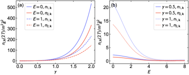
Figure 5: Particle numbers at the end of the $2T$ for each species of boson with (a) varying $\gamma$ and (b) varying $E$. For all these cases, the matrix $\eta=\left(\begin{array}[]{cc}1/2&1/6\\ 1/6&1/4\end{array}\right)$.

When $\tilde{g}\neq 0$, and $\tilde{g}$ is much smaller than the energy scale of $\hat{H}_{1}$, we can treat the interaction term perturbatively. By keeping the Dyson series to the first order, we have

$$\hat{U}_{1}^{\prime} = e^{-i\hat{H}_{1}^{\prime}t_{1}}$$ (42)

$$= e^{-i\hat{H}_{1}t_{1}}\left[1-i\tilde{g}\int_{0}^{t_{1}}\hat{V}(t)dt+O(U^{2})\right],$$

where $\hat{V}(t)=e^{i\hat{H}_{1}t}\hat{V}e^{-i\hat{H}_{1}t}$. Since $\hat{H}_{1}$ is a linear combination of the $\mathfrak{sp}(4,R)$ Lie algebra, according to Ref.[46, 45], the operator $\Psi_{\mathbf{k}}$ evolves as

$$e^{i\hat{H_{1}}t}\Psi_{\mathbf{k}}e^{-i\hat{H_{1}}t}=e^{-i\kappa\mathcal{H}_{1}t}\Psi_{\mathbf{k}}.$$ (43)

With this transformation, $\hat{V}(t)$ can be calculated. Then, the time evolution operator after two period of driving up to the first order in $\tilde{g}$ has the following form

$$\hat{U}(2T) = \hat{U}_{2}\hat{U}_{1}^{\prime}\hat{U}_{2}\hat{U}_{1}^{\prime}$$ (44)

$$= \left[1-i\tilde{g}\int_{0}^{t_{1}}dt\hat{A}\hat{V}(t)\hat{A}^{\dagger}\right.$$

$$\left.-i\tilde{g}\int_{0}^{t_{1}}dt\hat{A}^{2}\hat{V}(t)(\hat{A}^{\dagger})^{2}+O(\tilde{g}^{2})\right]\hat{A}^{2}$$

$$\equiv [1-i\tilde{g}\hat{\mathscr{V}}+O(\tilde{g}^{2})]\hat{A}^{2},$$

where we have defined $\hat{A}=e^{-i\hat{H}_{2}t_{2}}e^{-i\hat{H}_{1}t_{1}}$, and denoted the integral terms as $\hat{\mathscr{V}}$. Here, $\hat{A}\hat{V}(t)\hat{A}^{\dagger}$ and $\hat{A}^{2}\hat{V}(t)(\hat{A}^{\dagger})^{2}$ can also be calculated using the method in Eq.(43). As a result, the particle number at the end of the $2m$th period is given by

$$n_{i,\mathbf{k}}(2mT) = \langle 0|[\hat{U}^{\dagger}(2T)]^{m}\hat{n}_{i,\mathbf{k}}[\hat{U}(2T)]^{m}|0\rangle$$ (45)

$$= m^{2}\tilde{g}^{2}\langle 0|\hat{\mathscr{V}}^{\dagger}\hat{n}_{i,\mathbf{k}}\hat{\mathscr{V}}|0\rangle+O(\tilde{g}^{3})$$

where $\hat{n}_{i,\mathbf{k}}=a_{i,\mathbf{k}}^{\dagger}a_{i,\mathbf{k}}$. Here, we have used the relations $\hat{A}^{2}|0\rangle=-|0\rangle$ and $\hat{A}^{2}\hat{n}_{i,\mathbf{k}}(\hat{A}^{\dagger})^{2}=\hat{n}_{i,\mathbf{k}}$. Then, the expectation value part of above expression can be evaluated numerically. And we can conclude that the to the leading order, the particle numbers increase quadratically with interaction strengths $\tilde{g}$.

In Figure 5, we show the numerical results for the particle numbers $n_{i,\mathbf{k}}(2T)$ at the end of the second driving period varying with the parameters $E$ and $\gamma$ with $\eta_{ij}$ fixed. From Figure 5(a), we can see that for different fixed values of $E$, the particle numbers increase exponentially with increasing $\gamma$. However, the particle numbers decrease as the parameter $E$ increases. This result can be understood as follows: $\gamma$ controls the hopping between the excitations and the condensate in zero momentum. When increasing $\gamma$ with fixed kinetic term parameter $E$, more particles will be excited. Since the echo-breaking interactions are between the excited particles. Thus, more excited particles will result stronger echo-breaking effect. On the other hand, when increasing $E$ with fixed $\gamma$, the ratio $\gamma/E$ gets smaller, thus, the particles exciting is suppressed. Hence, the echo-breaking effect is weaker in this case.

VI Possible experiment implementation

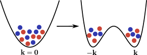
Figure 6: Schematics for the shaken optical lattice implementation of hopping terms between opposite momenta of two-component BEC Hamiltonian. Red and blue dots represent two species of bosons.

In previous sections, we explored a general driving protocol to facilitate quantum echo in two-component Bose-Einstein Condensates (BECs) and examined the impact of symmetry-breaking interactions on this phenomenon. In this section, we will propose a possible experiment implementation for this quantum echo.

The model Eq.(3) involves the hopping between the bosonic modes in opposite momenta $\pm\mathbf{k}$. The similar hopping also appears in the single-component BEC case and is proposed to be implemented in a double well structure in momentum space in Ref. [15]. This kind of double structure can be implemented in various experimental setups such as shaken optical lattice, spin-orbit coupling and periodic driving [15]. For the two-component case, we propose using a shaken optical lattice [61] as well. The experimental procedure would start with preparing a two-component BEC, initially condensing all particles in the zero momentum state. Subsequently, altering the band structure to form a double-well would populate the particles in opposite momenta as shown in Figure 6. This process corresponds to the hopping described in Equation (3) from opposite momenta.

In the second step of our driving protocol, the coupling term between opposite momenta disappear, however, the spin-orbit coupling terms like $a_{i,\mathbf{k}}^{\dagger}a_{j,\mathbf{k}}$ with $i\neq j$ are always present. Importantly, the implementation of spin-orbit coupling is also feasible in cold atom experiments [62]. Therefore, the driving protocol we propose can be effectively realized within the established frameworks of cold atom experimental setups.

VII Conclusion

In this paper, we have addressed the question of how quantum echo can be achieved in a two-component Bose-Einstein condensate system using the $Sp(4,R)$ group formalism. We have shown that under a periodic driving protocol consisting of two steps in each period, any $Sp(4,R)$ coherent state of two-component BEC can reverse to itself after two periods of driving. We have also developed a general method to construct the second-step Hamiltonian $\hat{H}_{2}$ from the first-step Hamiltonian $\hat{H}_{1}$ based on the property of real symplectic matrices and applied our method to two examples, one with time-independent $\hat{H}_{1}$ and one with time-dependent $\hat{H}_{1}$, then verified our theoretical prediction numerically. Furthermore, we have investigated how the interaction effect breaks the quantum echo process and found that the particle number deviation from the perfect revival is influenced by the ratio between the strengths of kinetic terms and interaction in the first-step Hamiltonian $\hat{H}_{1}$.

Our work extends the previous studies on quantum echo in single-component BEC and reveals new features of two-component BEC dynamics. Our work also showcases the usefulness and elegance of the $Sp(4,R)$ group formalism for studying quantum systems with real symplectic structures. Since our proof on the occurrence of quantum echo in two-component BEC system is solely based on the symplectic properties of the time evolution matrix, our result can also have potential use in spinor BEC and $N$-component boson system. Meanwhile, given the presence of real symplectic matrices in various areas of physical study [47, 48, 49, 50, 51, 52, 53, 54, 55, 56], we hope that our work will stimulate further research on this topic and inspire new applications of quantum echo in ultracold atom systems and beyond.

Appendix A The explicit expression of $\mathcal{U}_{0}$

In this appendix, we will give the explicit expression of $\mathcal{U}_{0}$ of the matrix $U_{0}=e^{\frac{i}{2}(\eta_{ij}Y^{ij}+\eta_{ij}^{*}Y_{ij})}$. The explicit form of the matrix generators $\{Y_{ij},Y^{ij},Y_{l}^{k}\}$ is [58]

$$(\kappa Y_{ij})_{ab}=\delta_{a,2+i}\delta_{b,j}+\delta_{a,2+j}\delta_{b,i},$$

$$(\kappa Y^{ij})_{ab}=\delta_{a,i}\delta_{b,2+j}+\delta_{a,j}\delta_{b,2+i},$$

$$(\kappa Y_{l}^{k})_{ab}=\delta_{a,k}\delta_{b,l}+\delta_{2+k,b}\delta_{2+l,a},$$ (46)

where $\kappa=\mathrm{diag}(1,1,-1,-1)$. Then, we define

$$\mathcal{A}=\frac{1}{2}\eta_{ij}Y^{ij}+\frac{1}{2}\eta_{ij}^{*}Y_{ij}.=\left(\begin{array}[]{cc}0&\eta\\ -\eta^{*}&0\end{array}\right).$$ (49)

According to Ref.[45], its eigenvalues are of the form $\{\lambda_{+},\lambda_{-},-\lambda_{+},-\lambda_{-}\}$, where

$$\lambda_{\pm}=\frac{1}{2}\sqrt{\mathrm{Tr}(\mathcal{A}^{2})\pm\sqrt{\mathrm{Tr}(\mathcal{A}^{2})^{2}-16\det(\mathcal{A})}}.$$ (50)

It can be calculated directly by Mathematica that $\mathcal{U}_{0}$ is given as

$$\mathcal{U}_{0,11} = \frac{|\eta_{11}|^{2}-|\eta_{22}|^{2}}{2(\lambda_{+}^{2}-\lambda_{-}^{2})}[\cos(\lambda_{-})-\cos(\lambda_{+})]+\frac{1}{2}[\cos(\lambda_{-})+\cos(\lambda_{+})],$$

$$\mathcal{U}_{0,12} = \frac{\eta_{11}\eta_{12}^{*}+\eta_{22}^{*}\eta_{12}}{\lambda_{+}^{2}-\lambda_{-}^{2}}[\cos(\lambda_{-})-\cos(\lambda_{+})],$$

$$\mathcal{U}_{0,21} = \frac{\eta_{11}^{*}\eta_{12}+\eta_{22}\eta_{12}^{*}}{\lambda_{+}^{2}-\lambda_{-}^{2}}[\cos(\lambda_{-})-\cos(\lambda_{+})],$$

$$\mathcal{U}_{0,22} = -\frac{|\eta_{11}|^{2}-|\eta_{22}|^{2}}{2(\lambda_{+}^{2}-\lambda_{-}^{2})}[\cos(\lambda_{-})-\cos(\lambda_{+})]+\frac{1}{2}[\cos(\lambda_{-})+\cos(\lambda_{+})].$$ (51)

If $\mathcal{U}_{0}$ is Hermitian, $\mathcal{U}_{0,11}$ and $\mathcal{U}_{0,22}$ should be real, meanwhile $\mathcal{U}_{0,12}=\mathcal{U}_{0,21}^{*}$. These conditions lead to that $\cos(\lambda_{+}),\cos(\lambda_{-})$ and $\lambda_{+}^{2}-\lambda_{-}^{2}$ should be real numbers. On the other hand, from Eq.(50), we have

$$\lambda_{+}^{2}-\lambda_{-}^{2} = \frac{1}{2}\sqrt{\mathrm{Tr}(\mathcal{A}^{2})^{2}-16\det(\mathcal{A})}$$ (52)

$$= \frac{1}{2}\sqrt{4(|\eta_{11}|^{2}+|\eta_{22}|^{2}+2|\eta_{12}|^{2})^{2}-16|\eta_{12}^{2}-\eta_{11}\eta_{22}|^{2}}$$

$$= \sqrt{(\eta_{11}|^{2}+|\eta_{22}|^{2}+2|\eta_{12}|^{2}+2|\eta_{12}^{2}-\eta_{11}\eta_{22}|)(\eta_{11}|^{2}+|\eta_{22}|^{2}+2|\eta_{12}|^{2}-2|\eta_{12}^{2}-\eta_{11}\eta_{22}|)}$$

$$\geq \sqrt{(\eta_{11}|^{2}+|\eta_{22}|^{2}+2|\eta_{12}|^{2}+2|\eta_{12}^{2}-\eta_{11}\eta_{22}|)(\eta_{11}|^{2}+|\eta_{22}|^{2}+2|\eta_{12}|^{2}-2|\eta_{12}|^{2}-2|\eta_{11}||\eta_{22}|)}$$

$$= \sqrt{(\eta_{11}|^{2}+|\eta_{22}|^{2}+2|\eta_{12}|^{2}+2|\eta_{12}^{2}-\eta_{11}\eta_{22}|)(\eta_{11}|^{2}-|\eta_{22}|^{2})^{2}}$$

$$\geq 0.$$

Hence, $\lambda_{+}^{2}-\lambda_{-}^{2}$ is real. Meanwhile, since $\mathrm{Tr}(\mathcal{A}^{2})=-2(|\eta_{11}|^{2}+|\eta_{22}|^{2}+2|\eta_{12}|^{2})$, according to Eq.(50), both $\lambda_{+}$ and $\lambda_{-}$ are imaginary. Thus, $\cos(\lambda_{+})$ and $\cos(\lambda_{-})$ are real. Hence, we have proven that $\mathcal{U}_{0}$ is a $2\times 2$ Hermitian matrix.

References

- Bloch [2005] I. Bloch, Ultracold quantum gases in optical lattices, Nature Phys 1, 23 (2005).
- Bloch et al. [2008] I. Bloch, J. Dalibard, and W. Zwerger, Many-body physics with ultracold gases, Rev. Mod. Phys. 80, 885 (2008).
- Chin et al. [2010] C. Chin, R. Grimm, P. Julienne, and E. Tiesinga, Feshbach resonances in ultracold gases, Rev. Mod. Phys. 82, 1225 (2010).
- Clark et al. [2017] L. W. Clark, A. Gaj, L. Feng, and C. Chin, Collective emission of matter-wave jets from driven Bose–Einstein condensates, Nature 551, 356 (2017).
- Feng et al. [2019] L. Feng, J. Hu, L. W. Clark, and C. Chin, Correlations in high-harmonic generation of matter-wave jets revealed by pattern recognition, Science 363, 521 (2019).
- Fu et al. [2018] H. Fu, L. Feng, B. M. Anderson, L. W. Clark, J. Hu, J. W. Andrade, C. Chin, and K. Levin, Density Waves and Jet Emission Asymmetry in Bose Fireworks, Phys. Rev. Lett. 121, 243001 (2018).
- Clark et al. [2015] L. W. Clark, L.-C. Ha, C.-Y. Xu, and C. Chin, Quantum Dynamics with Spatiotemporal Control of Interactions in a Stable Bose-Einstein Condensate, Phys. Rev. Lett. 115, 155301 (2015).
- Clark et al. [2016] L. W. Clark, L. Feng, and C. Chin, Universal space-time scaling symmetry in the dynamics of bosons across a quantum phase transition, Science 354, 606 (2016).
- Feng et al. [2018] L. Feng, L. W. Clark, A. Gaj, and C. Chin, Coherent inflationary dynamics for Bose–Einstein condensates crossing a quantum critical point, Nature Phys 14, 269 (2018).
- Fu et al. [2020] H. Fu, Z. Zhang, K.-X. Yao, L. Feng, J. Yoo, L. W. Clark, K. Levin, and C. Chin, Jet Substructure in Fireworks Emission from Nonuniform and Rotating Bose-Einstein Condensates, Phys. Rev. Lett. 125, 183003 (2020).
- Zhang et al. [2020] Z. Zhang, K.-X. Yao, L. Feng, J. Hu, and C. Chin, Pattern formation in a driven Bose–Einstein condensate, Nat. Phys. 16, 652 (2020).
- Hu et al. [2019] J. Hu, L. Feng, Z. Zhang, and C. Chin, Quantum simulation of Unruh radiation, Nat. Phys. 15, 785 (2019).
- Chen et al. [2020] Y.-Y. Chen, P. Zhang, W. Zheng, Z. Wu, and H. Zhai, Many-body echo, Phys. Rev. A 102, 011301 (2020).
- Lv et al. [2020] C. Lv, R. Zhang, and Q. Zhou, echoes for Breathers in Quantum Gases, Phys. Rev. Lett. 125, 253002 (2020).
- Lyu et al. [2020] C. Lyu, C. Lv, and Q. Zhou, Geometrizing Quantum Dynamics of a Bose-Einstein Condensate, Phys. Rev. Lett. 125, 253401 (2020).
- Zhang et al. [2022] J. Zhang, X. Yang, C. Lv, S. Ma, and R. Zhang, Quantum dynamics of cold atomic gas with SU(1,1) symmetry, Phys. Rev. A 106, 013314 (2022).
- Hahn [1950] E. L. Hahn, Spin Echoes, Phys. Rev. 80, 580 (1950).
- Myatt et al. [1997] C. J. Myatt, E. A. Burt, R. W. Ghrist, E. A. Cornell, and C. E. Wieman, Production of Two Overlapping Bose-Einstein Condensates by Sympathetic Cooling, Phys. Rev. Lett. 78, 586 (1997).
- Hall et al. [1998a] D. S. Hall, M. R. Matthews, J. R. Ensher, C. E. Wieman, and E. A. Cornell, Dynamics of Component Separation in a Binary Mixture of Bose-Einstein Condensates, Phys. Rev. Lett. 81, 1539 (1998a).
- Hall et al. [1998b] D. S. Hall, M. R. Matthews, C. E. Wieman, and E. A. Cornell, Measurements of Relative Phase in Two-Component Bose-Einstein Condensates, Phys. Rev. Lett. 81, 1543 (1998b).
- Modugno et al. [2002] G. Modugno, M. Modugno, F. Riboli, G. Roati, and M. Inguscio, Two Atomic Species Superfluid, Phys. Rev. Lett. 89, 190404 (2002).
- Papp et al. [2008] S. B. Papp, J. M. Pino, and C. E. Wieman, Tunable Miscibility in a Dual-Species Bose-Einstein Condensate, Phys. Rev. Lett. 101, 040402 (2008).
- Thalhammer et al. [2008] G. Thalhammer, G. Barontini, L. De Sarlo, J. Catani, F. Minardi, and M. Inguscio, Double Species Bose-Einstein Condensate with Tunable Interspecies Interactions, Phys. Rev. Lett. 100, 210402 (2008).
- McCarron et al. [2011] D. J. McCarron, H. W. Cho, D. L. Jenkin, M. P. Köppinger, and S. L. Cornish, Dual-species Bose-Einstein condensate of and , Phys. Rev. A 84, 011603 (2011).
- Lercher et al. [2011] A. D. Lercher, T. Takekoshi, M. Debatin, B. Schuster, R. Rameshan, F. Ferlaino, R. Grimm, and H. C. Nägerl, Production of a dual-species Bose-Einstein condensate of Rb and Cs atoms, Eur. Phys. J. D 65, 3 (2011).
- Pasquiou et al. [2013] B. Pasquiou, A. Bayerle, S. M. Tzanova, S. Stellmer, J. Szczepkowski, M. Parigger, R. Grimm, and F. Schreck, Quantum degenerate mixtures of strontium and rubidium atoms, Phys. Rev. A 88, 023601 (2013).
- Wacker et al. [2015] L. Wacker, N. B. Jørgensen, D. Birkmose, R. Horchani, W. Ertmer, C. Klempt, N. Winter, J. Sherson, and J. J. Arlt, Tunable dual-species Bose-Einstein condensates of and , Phys. Rev. A 92, 053602 (2015).
- Wang et al. [2015] F. Wang, X. Li, D. Xiong, and D. Wang, A double species 23Na and 87Rb Bose–Einstein condensate with tunable miscibility via an interspecies Feshbach resonance, J. Phys. B: At. Mol. Opt. Phys. 49, 015302 (2015).
- Trautmann et al. [2018] A. Trautmann, P. Ilzhöfer, G. Durastante, C. Politi, M. Sohmen, M. J. Mark, and F. Ferlaino, Dipolar Quantum Mixtures of Erbium and Dysprosium Atoms, Phys. Rev. Lett. 121, 213601 (2018).
- Ho and Shenoy [1996] T.-L. Ho and V. B. Shenoy, Binary Mixtures of Bose Condensates of Alkali Atoms, Phys. Rev. Lett. 77, 3276 (1996).
- Ho [1998] T.-L. Ho, Spinor Bose Condensates in Optical Traps, Phys. Rev. Lett. 81, 742 (1998).
- Ohmi and Machida [1998] T. Ohmi and K. Machida, Bose-Einstein Condensation with Internal Degrees of Freedom in Alkali Atom Gases, J. Phys. Soc. Jpn. 67, 1822 (1998).
- Esry et al. [1997] B. D. Esry, C. H. Greene, Jr. Burke, James P., and J. L. Bohn, Hartree-Fock Theory for Double Condensates, Phys. Rev. Lett. 78, 3594 (1997).
- Alon et al. [2008] O. E. Alon, A. I. Streltsov, and L. S. Cederbaum, Multiconfigurational time-dependent Hartree method for bosons: Many-body dynamics of bosonic systems, Phys. Rev. A 77, 033613 (2008).
- Ao and Chui [1998] P. Ao and S. T. Chui, Binary Bose-Einstein condensate mixtures in weakly and strongly segregated phases, Phys. Rev. A 58, 4836 (1998).
- Cirac et al. [1998] J. I. Cirac, M. Lewenstein, K. Mølmer, and P. Zoller, Quantum superposition states of Bose-Einstein condensates, Phys. Rev. A 57, 1208 (1998).
- Mertes et al. [2007] K. M. Mertes, J. W. Merrill, R. Carretero-González, D. J. Frantzeskakis, P. G. Kevrekidis, and D. S. Hall, Nonequilibrium Dynamics and Superfluid Ring Excitations in Binary Bose-Einstein Condensates, Phys. Rev. Lett. 99, 190402 (2007).
- Pu and Bigelow [1998] H. Pu and N. P. Bigelow, Properties of Two-Species Bose Condensates, Phys. Rev. Lett. 80, 1130 (1998).
- Timmermans [1998] E. Timmermans, Phase Separation of Bose-Einstein Condensates, Phys. Rev. Lett. 81, 5718 (1998).
- Micheli et al. [2003] A. Micheli, D. Jaksch, J. I. Cirac, and P. Zoller, Many-particle entanglement in two-component Bose-Einstein condensates, Phys. Rev. A 67, 013607 (2003).
- Tojo et al. [2010] S. Tojo, Y. Taguchi, Y. Masuyama, T. Hayashi, H. Saito, and T. Hirano, Controlling phase separation of binary Bose-Einstein condensates via mixed-spin-channel Feshbach resonance, Phys. Rev. A 82, 033609 (2010).
- Trippenbach et al. [2000] M. Trippenbach, K. Góral, K. Rzazewski, B. Malomed, and Y. B. Band, Structure of binary Bose-Einstein condensates, J. Phys. B: At. Mol. Opt. Phys. 33, 4017 (2000).
- Wang et al. [2010] C. Wang, C. Gao, C.-M. Jian, and H. Zhai, Spin-orbit coupled spinor bose-einstein condensates, Phys. Rev. Lett. 105, 160403 (2010).
- Kawaguchi and Ueda [2012] Y. Kawaguchi and M. Ueda, Spinor Bose–Einstein condensates, Physics Reports 520, 253 (2012).
- Wang and He [2022] C.-Y. Wang and Y. He, The quantum dynamics of two-component Bose–Einstein condensate: An symmetry approach, J. Phys.: Condens. Matter 34, 455401 (2022).
- Perelomov [1986] A. Perelomov, Generalized Coherent States and Their Applications (Springer-Verlag, Berlin Heidelberg, 1986).
- Weedbrook et al. [2012] C. Weedbrook, S. Pirandola, R. García-Patrón, N. J. Cerf, T. C. Ralph, J. H. Shapiro, and S. Lloyd, Gaussian quantum information, Rev. Mod. Phys. 84, 621 (2012).
- Simon [2000] R. Simon, Peres-Horodecki Separability Criterion for Continuous Variable Systems, Phys. Rev. Lett. 84, 2726 (2000).
- Simon et al. [1988] R. Simon, E. C. G. Sudarshan, and N. Mukunda, Gaussian pure states in quantum mechanics and the symplectic group, Phys. Rev. A 37, 3028 (1988).
- Colas et al. [2022] T. Colas, J. Grain, and V. Vennin, Four-mode squeezed states: Two-field quantum systems and the symplectic group , Eur. Phys. J. C 82, 6 (2022).
- Alhassid et al. [1983] Y. Alhassid, F. Gürsey, and F. Iachello, Group theory approach to scattering, Annals of Physics 148, 346 (1983).
- Deenen and Quesne [1985] J. Deenen and C. Quesne, Boson representations of the real symplectic group and their applications to the nuclear collective model, Journal of Mathematical Physics 26, 2705 (1985).
- Enayati et al. [2023] M. Enayati, J.-P. Gazeau, M. A. del Olmo, and H. Pejhan, Anti-de Sitterian ”massive” elementary systems and their Minkowskian and Newtonian limits (2023).
- Penna and Richaud [2017] V. Penna and A. Richaud, Two-species boson mixture on a ring: A group-theoretic approach to the quantum dynamics of low-energy excitations, Phys. Rev. A 96, 053631 (2017).
- Richaud and Penna [2017] A. Richaud and V. Penna, Quantum dynamics of bosons in a two-ring ladder: Dynamical algebra, vortexlike excitations, and currents, Phys. Rev. A 96, 013620 (2017).
- Charalambous et al. [2020] C. Charalambous, M. Á. García-March, G. Muñoz-Gil, P. R. Grzybowski, and M. Lewenstein, Control of anomalous diffusion of a Bose polaron, Quantum 4, 232 (2020).
- Pitaevskii and Stringari [2016] L. Pitaevskii and S. Stringari, Bose-Einstein Condensation and Superfluidity (Oxford University Press, 2016).
- Hasebe [2020] K. Hasebe, squeezing for Bloch four-hyperboloid via the non-compact Hopf map, J. Phys. A: Math. Theor. 53, 055303 (2020).
- Rowe et al. [1985] D. J. Rowe, G. Rosensteel, and R. Gilmore, Vector coherent state representation theory, Journal of Mathematical Physics 26, 2787 (1985).
- Coquereaux and Jadczyk [1990] R. Coquereaux and A. Jadczyk, Conformal theories, curved phase spaces, relativistic wavelets and the geometry of complex domains, Rev. Math. Phys. 02, 1 (1990).
- Parker et al. [2013] C. V. Parker, L.-C. Ha, and C. Chin, Direct observation of effective ferromagnetic domains of cold atoms in a shaken optical lattice, Nature Phys 9, 769 (2013).
- Galitski and Spielman [2013] V. Galitski and I. B. Spielman, Spin–orbit coupling in quantum gases, Nature 494, 49 (2013).