Fast convergence to an approximate solution by message-passing for complex optimizations

Abstract

Message-passing (MP) is a powerful tool for finding an approximate solution in optimization. We generalize it to nonlinear product-sum form, and numerically show the fast convergence for the minimum feedback vertex set and the minimum vertex cover known as NP-harp problems. From the linearity of MP in a logarithmic space, it is derived that an equilibrium solution exists in a neighborhood of random initial values. These results will give one of the reason why the convergence is very fast in collective computation based on a common mathematical background.

I Introduction

In complex optimization, one of the important issue is investigating how fast an approximate solution can be obtained. For example, by learning of connection weight parameters on a neural network, it is the task to search a target function from input to output in a high-dimensional pattern space in order to minimize the square error between output and teacher signals. In general, there are many local minima obtained by learning of neural network. Surprisingly, it has been shown with much interest that any target function can be realized in a sufficiently small neighborhood of random weight parameters on a neural network with sufficiently wide hidden layers through learning based on signal propagation [3, 4, 1, 2]. Instead of the complicated analysis [3, 4], as an intuitive explanation, the elementary proof has been presented by applying a linear theory [1, 2]. In other words, for the mapping function of input and output patterns, any solution exists in the neighborhood of random weights on a neural network, therefore the fast convergence is expected by learning of random neural network without wandering in the seach space forever.

On the other hand, from statistical physics approach, similar but different propagation methods called message-passing (MP) have been developed [5]. Although there are some types of MP with a same name: belief propagation (BP), they are not equivalent. One is well-known BP [6] to decode low-density parity-check codes [7] or to restore a damaged image on a graphical model [8, 5]. This type of MP is represented by sum-product or max-sum form [9]. Another is to approximately solve combinatorial optimization problems [10, 11]. That type of MP is represented by product-sum form as mentioned later. Through iterations of MP for minimizing a free-energy, the former performs propagation of a belief of state, while the later performs interactions among states. These different objectives may appear as sum-product or max-sum and product-sum forms, respectively. Here, a state means $\pm 1$ spin in Ising model [12, 5], or nodes’ label such as root identifier excluded in feedback vertex set (FVS) [11] or covered/uncovered node’s state as the candidate included/excluded in a set of vertex cover (VC) [10]. FVS is a set of nodes that are necessary to form loops, while VC is a set of covered nodes that are at least one of end-nodes for each link. Their approximate solutions are applicable to extract influencers [13] and to enhance robustness of connectivity [14] in complex networks. Theoretically an unique solution is assured by MP on only a tree, however practically a good solution is obtained by MP on a network with (long) loops in many cases. In general, on a loopy network, there can be many equilibrium solutions or sometimes more complex oscillations by MP depending on initial values.

In this paper, not only the fast convergence by MP in product-sum form is numerically shown, but also it is derived as a reason of fast convergence that the solution exists in a neighborhood of random initial values, based on a common mathematical background of linear theory [1]. We take particular note of that approximately solving optimization problems by MP and learning of neural network are related as propagation methods for collective computation, in spite of studying in different research fields of information science or machine learning and statistical physics or network science.

II Message-passing in product-sum form

We briefly review the statistical physics approaches [11, 10] to find approximate solutions for some of combinatorial optimizations such as the minimum FVS and VC problems. However, to seek common ground, the representations are slightly modified for generalizing them to MP in product-sum form. Note that the right-hand side in MP equation is updated by substituting the left-hand side, repeatedly.

II.1 For the minimum feedback vertex set

By using a cavity method [12, 5] for estimating the minimum FVS known as NP-hard [15], it is assumed that nodes $v\in\partial u$ are mutually independent of each other, when node $u$ is removed. Here, $\partial u$ denotes the set of connecting neighbor nodes of $u$. In the cavity graph, if all nodes $v\in\partial u$ are either empty ($A_{v}=0$) or roots ($A_{v}=v$), the added node $u$ can be a root ($A_{u}=u$). There are the following exclusive states [11].

State $A_{u}=0$:

$u$ is empty. Since $u$ is unnecessary as a root, it belongs to FVS.

State $A_{u}=u$:

$u$ becomes its own root.
The state $A_{v}=v$ of $v\in\partial u$ is changeable to $A_{v}=u$, when node $u$ is added.

State $A_{u}=w$:

one node $w\in\partial u$ becomes the root of $u$, when it is added, if $w$ is occupied and all other $w^{\prime}\in\partial u\backslash w$ are either empty or roots.

For a link $u\rightarrow v$, $v\in\partial u$, the corresponding probabilities to the above states are represented by the following MP equations [11].

$$q^{0}_{u\rightarrow v}=\frac{e^{-x}}{z^{FVS}_{u\rightarrow v}(t)}=\frac{\Pi_{w\in\partial u\backslash v}\sqrt[d_{u}-1]{e^{-x}}}{z^{FVS}_{u\rightarrow v}(t)},$$ (1)

$$q^{u}_{u\rightarrow v}=\frac{\Pi_{w^{\prime}\in\partial u\backslash v}\left(q^{0}_{w^{\prime}\rightarrow u}+q^{w^{\prime}}_{w^{\prime}\rightarrow u}\right)}{z^{FVS}_{u\rightarrow v}},$$ (2)

$$q^{w}_{u\rightarrow v}=\frac{(1-q_{w\rightarrow u}^{0})\Pi_{w^{\prime}\in\partial u\backslash v,w}(q_{w^{\prime}\rightarrow u}^{0}+q_{w^{\prime}\rightarrow u}^{w^{\prime}})}{z^{FVS}_{u\rightarrow v}},\;\;\;w\in\partial u\backslash v,$$ (3)

where $d_{u}$ denotes the degree of node $u$, $\partial u\backslash v$ is the subset of $\partial u$ except $v$, and $x>0$ is a parameter of inverse temperature to give a penalty $e^{-x}$ for minimizing the size of FVS. We have the normalization constant

$$z^{FVS}_{u\rightarrow v}\stackrel{{\scriptstyle\rm def}}{{=}}e^{-x}+\left\{\Pi_{w^{\prime}\in\partial u\backslash v}\left(q^{0}_{w^{\prime}\rightarrow u}+q^{w^{\prime}}_{w^{\prime}\rightarrow u}\right)\times\left(1+\sum_{w\in\partial u\backslash v}\frac{1-q^{0}_{w\rightarrow u}}{q^{0}_{w\rightarrow u}+q^{w}_{w\rightarrow u}}\right)\right\},$$ (4)

to satisfy

$$q^{0}_{u\rightarrow v}+q^{u}_{u\rightarrow v}+\sum_{w\in\partial u\backslash v}q^{w}_{u\rightarrow v}=1.$$ (5)

Note that there are $d_{u}-1$ links of $w^{\prime}\rightarrow u$ except $v\rightarrow u$, and that the multiplication term $\times 1$ of Eq.(5) is hidden in the numerator of the right-hande side of Eq.(1). $1-q^{0}_{w\rightarrow u}=q^{1}_{w\rightarrow u}+\sum_{w^{\prime}\in\partial w\backslash u}q^{*w^{\prime}}_{w\rightarrow u}$ is also a sum form. Thus, the right-hande sides of Eqs. (1)(2)(3) are product-sum forms.

The $0$ state probability of $u$ included in FVS is given by [11]

$$q_{u}^{0}\stackrel{{\scriptstyle\rm def}}{{=}}\frac{e^{-x}}{e^{-x}+\left\{1+\sum_{w\in\partial i}\frac{1-q_{w\rightarrow u}^{0}}{q_{w\rightarrow u}^{0}+q_{w\rightarrow u}^{w}}\right\}\Pi_{v\in\partial i}\left(q_{v\rightarrow u}^{0}+q_{v\rightarrow u}^{v}\right)}.$$ (6)

II.2 For the minimum vettex cover

In the cavity graph for estimating the minimum VC known as NP-hard [15], since at least one end-node of each link should be covered, the following three exclusive states at node $u$ are considered for a link $u\rightarrow v$, $v\in\partial u$ [10].

Sate $0$:

$u$ is uncoverd, when there are no uncovered nodes $w\in\partial u\backslash v$.

Sate $1$:

$u$ is coverd, when two or more nodes $w\in\partial u\backslash v$ are uncovered.

Sate $*w$:

As joker state, $u$ is sometimes covered and sometimes uncovered, when only one node $w\in\partial u\backslash v$ is uncovered but other $w^{\prime}\in\partial u\backslash v,w$ are covered or joker states.

The corresponding probabilities are represented by the following MP equations [10].

$$q^{0}_{u\rightarrow v}=\frac{\Pi_{w^{\prime}\in\partial u\backslash v}(1-q^{0}_{w^{\prime}\rightarrow u})}{z^{VC}_{u\rightarrow v}},$$ (7)

$$q^{1}_{u\rightarrow v} = \frac{e^{-x}\left[1-\Pi_{w^{\prime}\in\partial u\backslash v}(1-q^{0}_{w^{\prime}\rightarrow u})-\sum_{w\in\partial u\backslash v}q^{0}_{w\rightarrow u}\Pi_{w^{\prime}\in\partial u\backslash v,w}(1-q^{0}_{w^{\prime}\rightarrow u})\right]}{z^{VC}_{u\rightarrow v}},$$ (8)

$$= \frac{\Pi_{w^{\prime}\in\partial u\backslash v}\sqrt[d_{u}-1]{e^{-x}\mbox{(the numerator of above equation)}}}{z^{VC}_{u\rightarrow v}},$$

$$q^{*w}_{u\rightarrow v} = \frac{e^{-x}q^{0}_{w\rightarrow u}\Pi_{w^{\prime}\in\partial u\backslash v,w}(1-q^{0}_{w^{\prime}\rightarrow u})}{z^{VC}_{u\rightarrow v}},$$ (9)

$$= \frac{\sqrt[d_{u}-1]{e^{-x}}q^{0}_{w\rightarrow u}\Pi_{w^{\prime}\in\partial u\backslash v,w}\left[\sqrt[d_{u}-1]{e^{-x}}(1-q^{0}_{w^{\prime}\rightarrow u})\right]}{z^{VC}_{u\rightarrow v}},\;\;\;w\in\partial u\backslash v,$$

with the normalization constant

$$z^{VC}_{u\rightarrow v}\stackrel{{\scriptstyle\rm def}}{{=}}e^{-x}\left[1-(1-e^{x})\Pi_{w^{\prime}\in\partial u\backslash v}(1-q^{0}_{w^{\prime}\rightarrow u})\right],$$ (10)

to satisfy $q^{0}_{u\rightarrow v}+q^{1}_{u\rightarrow v}+\sum_{w\in\partial u\backslash v}q^{*w}_{u\rightarrow v}=1$. From this normalization condition and $1-q_{u\rightarrow v}^{0}=q^{1}_{u\rightarrow v}+\sum_{w\in\partial u\backslash v}q^{*w}_{u\rightarrow v}$, the right-hand sides of Eqs.(7)(9) are product-sum forms. The right-hand sides of Eqs.(8) may be not exactly the form. However, Eq.(7) is essential and other ancillary Eqs.(8)(9) are not, since $z^{VC}_{u\rightarrow v}$ in Eq.(10) is represented by only the $0$ state’s probabilities.

The $1$ state probability of $u$ included in VC is given by [10]

$$q_{u}^{1}\stackrel{{\scriptstyle\rm def}}{{=}}\frac{e^{-x}\left\{1-\Pi_{v\in\partial u}(1-q_{v\rightarrow u}^{0})-\sum_{w\in\partial u}q_{w\rightarrow u}^{0}\Pi_{w^{\prime}\in\partial u\backslash w}(1-q_{w^{\prime}\rightarrow u}^{0})\right\}}{e^{-x}\left\{1-(1-e^{x})\Pi_{v\in\partial u}(1-q_{v\rightarrow u}^{0})\right\}}.$$ (11)

II.3 For more general cases

We consider a set $\Omega_{u}=\{\alpha_{u},\beta_{u},\gamma_{u},\ldots,\kappa_{u},\ldots,\omega_{u}\}$ of states in any order. The number $|\Omega_{u}|$ can be different for each node $u$. In the case of minumum FVS, the states are $\alpha_{u}=0$, $\beta_{u}=u$, and $\gamma_{u},\ldots,\omega_{u}\in\partial u\backslash v$. In the case of minumum VC, the states are $\alpha_{u}=0$, and $\gamma_{u},\ldots,\omega_{u}$ are jokers $*$ of $w\in\partial u\backslash v$. $\beta_{u}=1$ is an exception by $q_{u\rightarrow v}^{1}=1-(q^{0}_{u\rightarrow v}+\sum_{w\in\partial u\backslash v}q^{*w}_{u\rightarrow v})$.

Then, by an inspiration from Ref. [16], Eqs. (1)(2)(3)(4) or Eqs. (7)(9)(10) are generalized as MP in product-sum form. In the following example, we set that only one state $\alpha_{u}$ has a penalty term $e^{-x}$ to minimize its probability.

$$q^{\alpha_{u}}_{u\rightarrow v}(t+1) = \frac{e^{-x}}{z_{u\rightarrow v}(t)}\Pi_{w^{\prime}\in\partial u\backslash v}\left(\sum_{\delta\in S_{\alpha_{u}}}q^{\delta}_{w^{\prime}\rightarrow u}(t)\right),$$ (12)

$$= \frac{1}{z_{u\rightarrow v}(t)}\Pi_{w^{\prime}\in\partial u\backslash v}\left(\sqrt[d_{u}-1]{e^{-x}}\sum_{\epsilon\in S_{\alpha_{u}}}q^{\epsilon}_{w^{\prime}\rightarrow u}(t)\right),$$

$$\hskip 56.9055pt\vdots$$

$$q^{\kappa_{u}}_{u\rightarrow v}(t+1)=\frac{1}{z_{u\rightarrow v}(t)}\Pi_{w^{\prime}\in\partial u\backslash v}\left(\sum_{\delta^{\prime}\in S_{\kappa_{u}}}q^{\delta^{\prime}}_{w^{\prime}\rightarrow u}(t)\right),$$ (13)

$$\hskip 56.9055pt\vdots$$

$$q^{\omega_{u}}_{u\rightarrow v}(t+1)=\frac{1}{z_{u\rightarrow v}(t)}\Pi_{w^{\prime}\in\partial u\backslash v}\left(\sum_{\delta^{\prime\prime}\in S_{\omega_{u}}}q^{\delta^{\prime\prime}}_{w^{\prime}\rightarrow u}(t)\right),$$ (14)

where $S_{\alpha_{u}},\ldots,S_{\kappa_{u}},\ldots,S_{\omega_{u}}\subset\Omega_{u}$, $w^{\prime}\in\partial u\backslash v$, and $z_{u\rightarrow v}(t)$ is defined to satisfy the normalization condition $\sum_{\kappa_{u}\in\Omega_{u}}q^{\kappa_{u}}_{u\rightarrow v}(t)=1$ at each time $t$. We emphasize the dependence of iteration time step $t\geq 0$ in the representation of Eqs. (12)(13)(14).

III Numerical and theoretical analysises

III.1 Simulation results for fast convergence of MP

We numerically investigate the convergence of MP Eqs. (1)(2)(3) or (7)(8)(9) for the minimum FVS or VC problem. It is evaluated by the cosine similarity $Sim(t)$ between the state probabilities at iteration times $t-1$ and $t$,

$$Sim(t)\stackrel{{\scriptstyle\rm def}}{{=}}\frac{\sum_{u=1}^{N}\sum_{e:u\rightarrow v}\sum_{\kappa_{u}\in\Omega_{u}}q_{e}^{\kappa_{u}}(t-1)\times q_{e}^{\kappa_{u}}(t)}{\sqrt{\sum_{u=1}^{N}\sum_{e:u\rightarrow v}\sum_{\kappa_{u}\in\Omega_{u}}q_{e}^{\kappa_{u}}(t-1)^{2}}\times\sqrt{\sum_{u=1}^{N}\sum_{e:u\rightarrow v}\sum_{\kappa_{u}\in\Omega_{u}}q_{e}^{\kappa_{u}}(t)^{2}}}.$$

When $Sim(T)$ approaches to $1$, the state probabilities $\{q_{e}^{\kappa_{u}}(T)\}$ converge around a time $T$.

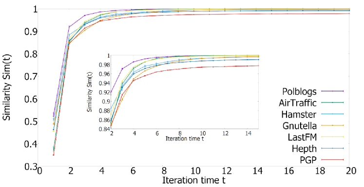
Figure 1: Similarity between the state probabilities at iteration times $t-1$ and $t$ by simple MP for the minimum FVS in real networks distinguished by color lines. Inset show the enlarged part to see the convergent curves.

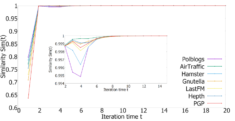
Figure 2: Similarity between the state probabilities at iteration times $t-1$ and $t$ by simple MP for the minimum VC in real networks distinguished by color lines. Inset show the enlarged part to see the convergent curves.

Table 1: Data source. Name of network, numbers $N$, $M\stackrel{{\scriptstyle\rm def}}{{=}}\sum_{u=1}^{N}d_{u}/2$ of nodes and links, diameter $D$ as the maximum shortest path length between two nodes, access destination. Polblogs $\sim$ PGP are Scale-Free networks whose degree distributions follow power-law, while Cost2666 and Janos-us-ca are planar communication networks.

Name	$N$	$M$	$D$	URL
Polblogs	1222	16714	8	http://www-personal.umich.edu/$\sim$mejn/netdata/
AirTraffic	1226	2408	17	https://data.europa.eu/data/datasets
				/12ec37d3-ada7-4d4c-84ef-f347b1d8dedf?locale=fi
Hamster	1788	12476	14	https://networkrepository.com/soc-hamsterster.php
Gnutella	6299	20776	9	http://snap.stanford.edu/data/p2p-Gnutella08.html
LastFM	7624	278060	15	http://snap.stanford.edu/data/feather-lastfm-social.html
Hepth	8638	24806	18	http://snap.stanford.edu/data/ca-HepTh.html
PGP	10680	24316	24	https://deim.urv.cat/$\sim$alexandre.arenas/data/welcome.htm
Cost266	37	56	8	http://sndlib.zib.de/download/sndlib-networks-native.zip
Janos-us-ca	39	61	10	http://sndlib.zib.de/download/sndlib-networks-native.zip

Table 2: Cosine similarities between $\{q_{e}^{\kappa_{u}}(T^{*})\}$ and $\{\tilde{q}_{e}^{\kappa_{u}}(0)\}$ (1st column), and between $\{q_{e}^{\kappa_{u}}(T^{*})\}$ and $\{\tilde{q}_{e}^{\kappa_{u}}(T^{*})\}$ (2nd column). The results are averaged over 100 samples.

(a) FVS

	Polblog	Airtraffic	Hamster	GNUtella	LastFM	Hepth	PGP
$\{q_{e}^{\kappa_{u}}(T^{*})\}$ and $\{\tilde{q}_{e}^{\kappa_{u}}(0)\}$	0.768	0.883	0.874	0.936	0.934	0.949	0.877
$\{q_{e}^{\kappa_{u}}(T^{*})\}$ and $\{\tilde{q}_{e}^{\kappa_{u}}(T^{*})\}$	0.998	0.993	0.998	0.998	0.995	0.997	0.996

(b) VC

	Polblog	Airtraffic	Hamster	GNUtella	LastFM	Hepth	PGP
$\{q_{e}^{\kappa_{u}}(T^{*})\}$ and $\{\tilde{q}_{e}^{\kappa_{u}}(0)\}$	0.770	0.879	0.864	0.944	0.940	0.944	0.960
$\{q_{e}^{\kappa_{u}}(T^{*})\}$ and $\{\tilde{q}_{e}^{\kappa_{u}}(T^{*})\}$	0.988	0.991	0.998	0.995	0.996	0.997	0.994

The following results are averaged over 100 samples from initial $\{q_{e}^{\kappa_{u}}(0)\}$ of uniform random numbers in the interval $(0,1)$. We set the parameter of inverse temperature as $x=7$. Note that the unit time consists of the updating by MP in order of random permutations of $N$ nodes and $d_{u}$ links to avoid vibration behaviour as few as possible instead of synchronously simultaneous updating of all.

Figures 1 and 2 show the time evolutions of $Sim(t)$ by MP for the minimum FVS and VC problems, respectively, on real networks with thousands nodes and links as shown in Table 1. Each colored curves are quickly converged until only several iterations less than around ten. Moreover, the variance indicated by vertical line is very small in 100 samples. Such small variance on each colored line means that similar $Sim(t)$ is obtained at each time $t$ from any initial value, because the time-course can reach an equilibrium solution in the neighborhood of random initial value as discussed in the next section. In other words, without almost depending on the topological difference, $Sim(t)$ behaves similarly even for the convergence to different equilibrium solutions which depend on initial values. On the other hand, there are different shapes of curves for FVS and VC in Figs. 1 and 2. Depending on data in Table 1, these colored curves are also slightly different in each of Figs. 1 and 2. The tested networks are Scale-Free (SF) commonly but with different total numbers $N$, $M$ of nodes and links, and the diameter $D$. Other topological properties may be different, however not only huge candidates of topological measures can be considered such as clustering coefficient, average length of the shortest paths, degree-degree correlations, modularity or motifs, and so on, but also it is unestimable which are determinant in advance. The reasons of different shapes of curves are considered from the differences of sum terms or of number of states with penalty in Eqs. (1)(2)(3) and (7)(8)(9) and of some topological properties, although the detail mechanism are unknown at the current stage. Note that these number of products are same as $d_{u}-1$ links at node $u$.

In addition, the existing of equilibrium solution is investigated by random perturbation for Figs. 1 and 2. After obtaining an convergent $\{q_{e}^{\kappa_{u}}(T^{*})\}$ from any $\{q_{e}^{\kappa_{u}}(0)\}$ of uniform random numbers in the interval $(0,1)$, another $\{\tilde{q}_{e}^{\kappa_{u}}(0)\}$ is set by adding uniform random numbers in the interval $(-\varepsilon,\varepsilon)$ to $\{q_{e}^{\kappa_{u}}(T^{*})\}$. From $\{\tilde{q}_{e}^{\kappa_{u}}(0)\}$, the corresponding convergent $\{\tilde{q}_{e}^{\kappa_{u}}(T^{*})\}$ is recalculated. Then, we compute the cosine similarities between $\{q_{e}^{\kappa_{u}}(T^{*})\}$ and $\{\tilde{q}_{e}^{\kappa_{u}}(0)\}$, and between $\{q_{e}^{\kappa_{u}}(T^{*})\}$ and $\{\tilde{q}_{e}^{\kappa_{u}}(T^{*})\}$. The increased similarities from first to second columns in Table 2(a)(b) exhibit that, as equilibrium solutions, same convergent values are almost reached from the neighborhood of them. Here, we set a sufficient large iteration time $T^{*}=100$ and a small perturbation parameter $\varepsilon=0.4$. Note that we have also similar results of slightly larger similarities for $\varepsilon=0.2$ as closer $\{\tilde{q}_{e}^{\kappa_{u}}(0)\}$ to $\{q_{e}^{\kappa_{u}}(T^{*})\}$. For Figs. 1 and 2, it is intractable to more regorously analyze the stabilities even under a special perturbation of Gaussian distribution, because the sizes of Jacobian matrix [10] are too large in the linear approximations of Eqs. (1)(2)(3) and (7)(8)(9) as nonlinear mappings around equilibrium solutions whose number is unknown. In the case of FVS, some extensions are required involving complex calculations with not only $0$ states in the case of VC but also other $u$ and $w$ states, $w\in\partial u\backslash v$, the analysis will be a further study. However, for Cost266 and Janos-us-ca with small sizes in Table 1, we calculate it in the case of VC which has only essential variables of $0$ states. Under the perturbation of Gaussian distribution in applying the derivation for VC [10], we confirm the stabilities of equilibrium solutions by obtaining that the largest eigenvalues of the following Jacobian matrix $J$ are less than $1$ for all $100$ trials of random initial values after $T^{*}=10$, $100$, and $1000$ iterations, respectively.

$$J_{u\rightarrow v,w\rightarrow u}\stackrel{{\scriptstyle\rm def}}{{=}}\left\{\frac{e^{-x}\Pi_{w^{\prime}\in\partial u\backslash v,w}(1-q_{w^{\prime}\rightarrow u}^{0}(T^{*}))}{(z_{u\rightarrow v}^{VC}(T^{*}))^{2}}\right\}^{2},\;\;\;\text{for}\;\;w\in\partial u\backslash v,$$

$$J_{u\rightarrow v,w\rightarrow u^{\prime}}\stackrel{{\scriptstyle\rm def}}{{=}}0,\;\;\;\text{otherwise for}\;\;u^{\prime}\neq u,\;u^{\prime}=u\;\text{and}\;w=v,\;\text{or}\;u^{\prime}=u\;\text{and}\;w\notin\partial u.$$

If an equilibrium solution (or very close solutions) is obtained by MP even from different initial values, it may be difficult to distinguish the nodes included or excluded in FVS or VC by ambiguous values of $0<q_{u}^{0}$ or $q_{u}^{1}<1$. Thus, in practical point of view, decimation process [11] is usually performed for finding the candidate of FVS or VC one by one (or the candidates of some nodes at once for efficiency), in which the unit time consists of $T>1$ rounds of updating by MP in order of random permutations of $N$ nodes and $d_{u}$ links. At each time by decimation process, the selected node $u$ with the highest $q_{u}^{0}$ or $q_{u}^{1}$ defined by Eq.(6) or (11) is removed as candidate of FVS or VC. As the candidates, we can also select the highest top dozens of nodes at once. After removing the selected nodes, $T$ rounds of updating are performed again at next time. Such process is repeated until satisfying the condition of no loop or covering one of end-nodes for each link. The obtained results with decimation are labels $0/1$ of nodes included/excluded in FVS or VC, they may differ form an equilibrium solution with ambiguous values in $(0,1)$ by simple MP without decimation.

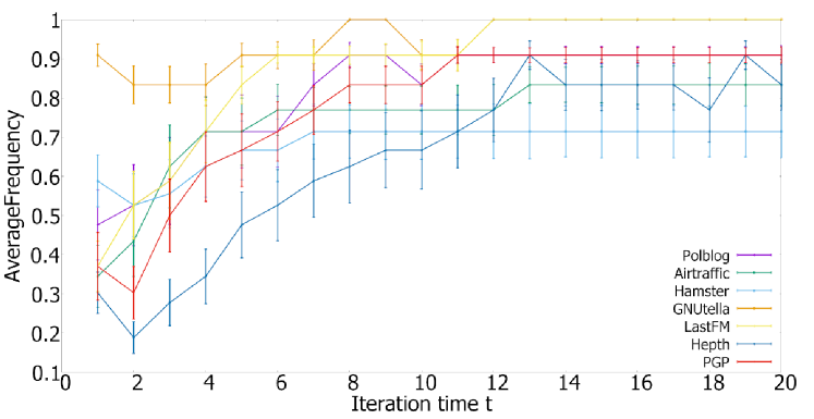
Figure 3: Average frequency of selected nodes as FVS in top 10 by MP with decimation in real networks distinguished by color lines. The vertical bar denotes the variance over 100 samples.

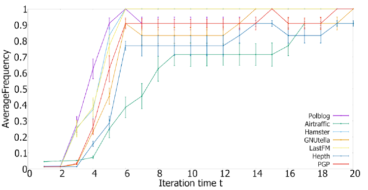
Figure 4: Average frequency of selected nodes as VC in top 10 by MP with decimation in real networks distinguished by color lines. The vertical bar denotes the variance over 100 samples.

Figures 3 and 4 show the time evolution of average frequency of selected nodes in the highest top 10 at time $t$ by MP with decimation over 100 samples of different random initial values. Commonly, the frequency tends to increase as larger $t$, however there are slightly different shapes of curves with different lengths of bars as the variances. For these differences, the reasons are also considered from the differences of sum terms or of number of states with penalty in Eqs. (1)(2)(3) and (7)(8)(9) and of some topological properties. Here, the maximum frequency $\frac{100}{100}$ means that all selected nodes are completely overlapped, while the minimum frequency $\frac{1}{100}$ means that selected nodes are non-overlapped and appeared for only one sample. A value between the maximum and the minimum gives the commonality of nodes selected with decimation over samples. In other words, it is corresponded to the variety of intermediate stages until reaching a solution in ranging from unique to quite different according to initial values.

In fact, as visualized examples in Fig. 5 from top to bottom, different sets of VC are found by decimation process for $T=10$ on real communication networks (see Table 1). The candidate node is chosen one by one at each time. Consequently, the solutions of VC depend on initial values of state probabilities. Note that the feasible solution by MP with decimation [10] is nearly optimal [13], since its size is almost half of that by a 2-approximation algorithm theoretically guaranteed in computer science [17].

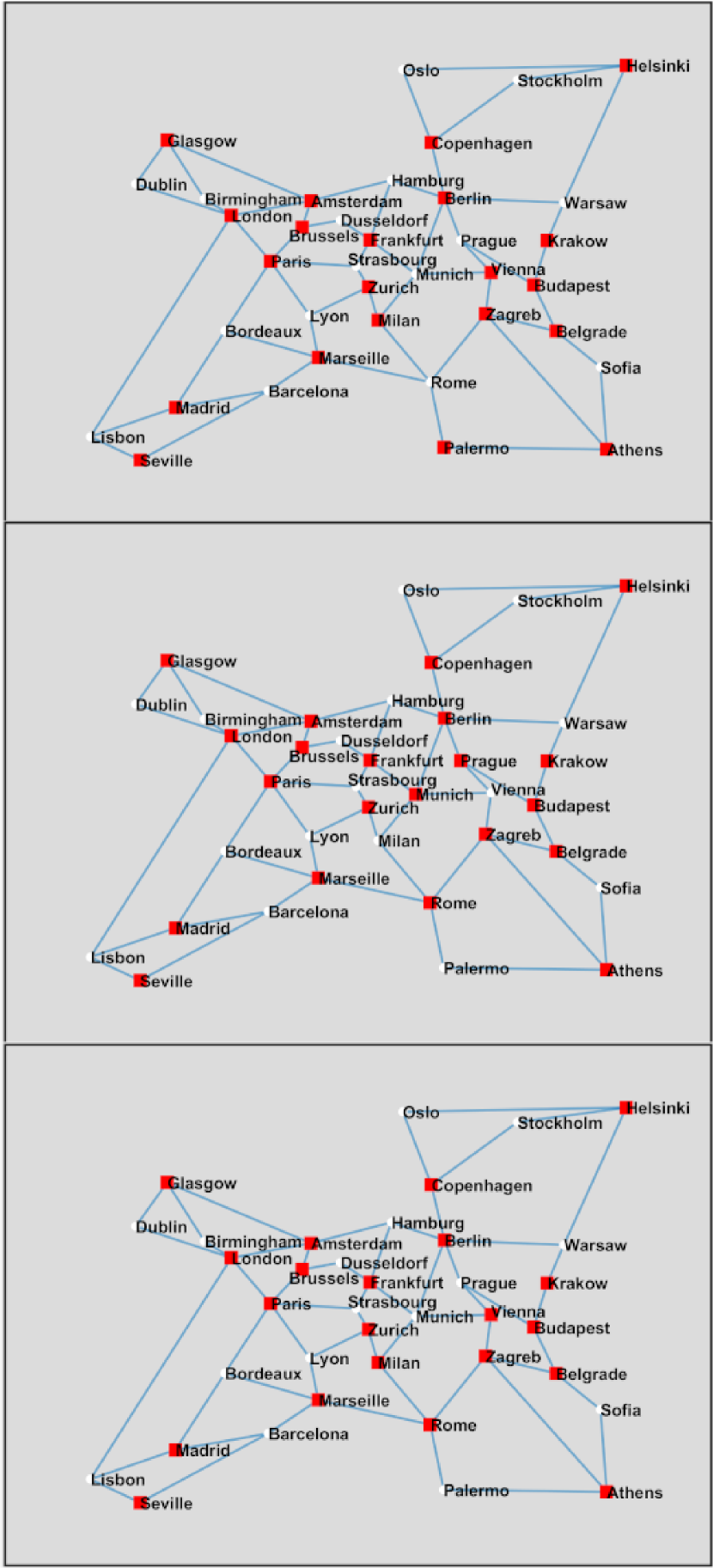
(a) Cost266

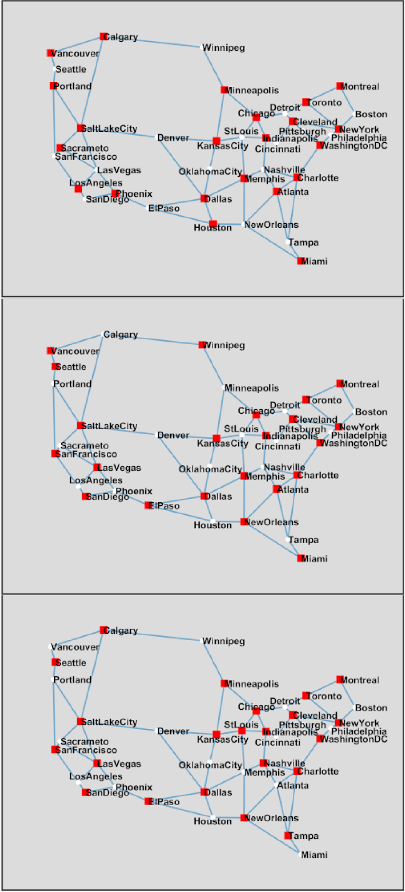
(b) Janos-us-ca

Figure 5: Different sets of VC colored by red from top to bottom according to initial values on real communication networks in (a) EU and (b) USA.

III.2 Linear theory for mesagge-passing in product-sum form

In this subsection, for MP Eqs. (12)(13)(14) in product-sum form without round and decimation process, we study how far is the equilibrium solution from initial values in the logarithmic space of state probabilities $\{q_{e}^{\kappa_{u}}\}$. Since Eqs. (12)(13)(14) are generalizations of Eqs. (1)(2)(3) or Eqs. (7)(9), the same discussion is true for the case of minimum FVS [11] or VC [10]. The linear theory is applied by a similar but slightly different way to learning of multilayer neural networks [1] (See Appendix A.1 for the brief review). In advance, we should take care of that only the existence of solution is discussed in a neighborhood of random initial values without taking into account dynamics of the trajectory to it as similar to the case of learning of neural networks [1].

To eliminate the denominator $z_{u\rightarrow v}$ of partition function in the right-hand side of Eqs. (12)(13)(14), we consider the logarithm of ratio $q_{e:u\rightarrow v}^{\kappa_{u}}(t+1)/q_{e:u\rightarrow v}^{\omega_{u}}(t+1)$ in the left-hand side. Then, from the right-hand side,

$$b_{\varepsilon}(t)\stackrel{{\scriptstyle\rm def}}{{=}}\sum_{w^{\prime}\in\partial u\backslash v}\log\left(\frac{\sum_{\delta^{\prime}_{u}\in S_{\kappa_{u}}}q_{w^{\prime}\rightarrow u}^{\delta^{\prime}_{u}}(t)}{\sum_{\delta^{\prime\prime}_{u}\in S_{\omega_{u}}}q_{w^{\prime}\rightarrow u}^{\delta^{\prime\prime}_{u}}(t)}\right),$$ (15)

is obtained as each element of $K$-dimensional vector $\bm{b}(t)$. The number $\varepsilon$ depends on link $e:u\rightarrow v$ and state $\kappa_{u}\in\Omega_{u}\backslash\omega_{u}$. There exist $d_{u}$ links emanated from node $u$, which has $|\Omega_{u}|$ states. The total number $K$ of variables is $\sum_{u=1}^{N}d_{u}\times(|\Omega_{u}|-1)$, where $-1$ is the reducing due to the denominator w.r.t $\omega_{u}$ in each element of $\bm{b}(t)$. In the cases of minimum FVS or VC, the states are $0$, $u$ or exception $1$, and $w$ or $*w$, $w\in\partial u\backslash v$, we have $|\Omega_{u}|-1=1+1+d_{u}-1-1=d_{u}$ or $d_{u}-1$ and therefore $K=\sum_{u=1}^{N}d_{u}^{2}$ or $\sum_{u=1}^{N}d_{u}(d_{u}-1)$.

We also consider a $(K+2M)$-dimensional vector

$$\bm{y(t)} \stackrel{{\scriptstyle\rm def}}{{=}} \left\{\log q_{e_{1}}^{\alpha_{1}}(t+1),\ldots,\log q_{e_{1}}^{\omega_{1}}(t+1),\ldots,\log q_{e}^{\alpha_{u}}(t+1),\ldots,\log q_{e}^{\omega_{u}}(t+1),\right.$$ (16)

$$\left.\ldots,\log q_{e_{2M}}^{\alpha_{N}}(t+1),\ldots,\log q_{e_{2M}}^{\omega_{N}}(t+1),\right\},$$

and a $K\times(K+2M)$ block-diagonal matrix ${\cal Q}$, whose submatrix is same as

$$Q_{(e)}\stackrel{{\scriptstyle\rm def}}{{=}}\left[\begin{array}[]{ccccc}1&0&\ldots&0&-1\\ 0&1&\ldots&0&-1\\ \vdots&\vdots&\ddots&\vdots&\vdots\\ 0&0&\ldots&1&-1\end{array}\right]$$ (17)

except the size $(|\Omega_{u}|-1)\times|\Omega_{u}|$ for link $e:u\rightarrow v$.

Based on the above preparations, the logarithm of ratio of Eqs. (12) or (13) and (14) becomes the following systems of linear equations.

$$\begin{pmatrix}\boxed{Q_{(e_{1})}}&&&&\\ &\ddots&&\text{\huge{0}}&\\ &&\boxed{Q_{(e)}}&&\\ &\text{\huge{0}}&&\ddots&\\ &&&&\boxed{Q_{(e_{2M})}}\end{pmatrix}\left(\begin{array}[]{c}\log q_{e_{1}}^{\alpha_{1}}(t+1)\\ \vdots\\ \log q_{e_{1}}^{\omega_{1}}(t+1)\\ \vdots\\ \log q_{e}^{\alpha_{u}}(t+1)\\ \vdots\\ \log q_{e}^{\omega_{u}}(t+1)\\ \vdots\\ \log q_{e_{2M}}^{\alpha_{N}}(t+1)\\ \vdots\\ \log q_{e_{2M}}^{\omega_{N}}(t+1)\end{array}\right)=\left(\begin{array}[]{c}b_{1}(t)\\ \vdots\\ b_{\varepsilon}(t)\\ \vdots\\ b_{K}(t)\end{array}\right).$$

We assume that directional links are properly ordered as $e_{1}:1\rightarrow v^{\prime}\neq 1,\ldots,e:u\rightarrow v,\ldots,e_{2M}:N\rightarrow v^{\prime\prime}\neq N$ with numbering nodes from $1$ to $N$. Note that the $\pm 1$ elements of ${\cal Q}_{(e)}$ correspond to $+\log q_{e}^{\kappa_{u}}(t+1)$ and $-\log q_{e}^{\omega_{u}}(t+1)$ as the state probability and the constraint of normalization, respectively, for each link. As the matrix-vector form, we have

$${\cal Q}\bm{y}(0)=\bm{b}(0),$$ (18)

$${\cal Q}\bm{y}(\infty)=\bm{b}(\infty),$$ (19)

where $\{q_{u\rightarrow v}^{\kappa_{u}}(\infty)\}$ means an equilibrium solution for MP Eqs. (12)(13)(14). Note that the topological network structure is embedded in ${\cal Q}$ whose block-diagonal sizes are allocated by $|\Omega_{u}|-1$ ($=d_{u}$ or $d_{u}-1$: number of links at $u$ in the case of the minimum FVS or VC) of the submatrix ${\cal Q}_{(e)}$ for links $e:u\rightarrow v$, $u=1,2,\ldots,N$, and its connecting neighbor nodes $v\in\partial u$.

By substituting Eq.(18) from Eq.(19), we have

$${\cal Q}\bm{\Delta y}=\bm{b}(\infty)-\bm{b}(0)\stackrel{{\scriptstyle\rm def}}{{=}}\bm{\Delta b},$$ (20)

where $\varepsilon$-th element of $\bm{\Delta y}\stackrel{{\scriptstyle\rm def}}{{=}}\bm{y}(\infty)-\bm{y}(0)$ is $\Delta y_{\varepsilon}=\log r_{e}^{\kappa_{u}}$ from introducing the change rate $r_{e}^{\kappa_{u}}\stackrel{{\scriptstyle\rm def}}{{=}}q_{e}^{\kappa_{u}}(\infty)/q_{e}^{\kappa_{u}}(1)$ and

$$\log q_{e}^{\kappa_{u}}(\infty)=\log q_{e}^{\kappa_{u}}(1)+\log r_{e}^{\kappa_{u}}.$$

Remember the definition of $\bm{y}(t)$ by Eq.(16).

When we consider a vector $\bm{n^{(q)}}$ in the null space $\{\bm{n}|{\cal Q}\bm{n}=\bm{0},\bm{n}\geq\bm{0}\}$ of ${\cal Q}$, $\bm{\Delta y}+\bm{n^{(q)}}$ is also the solution of Eq.(20) because of ${\cal Q}(\bm{\Delta y}+\bm{n^{(q)}})=\bm{\Delta b}$. Since there is only one pair of $\pm 1$ elements in each row of ${\cal Q}$, $\bm{n^{(q)}}$ is uniquely determined as $\bm{n^{(q)}}=\{c_{e_{1}},\ldots,c_{e_{1}},\ldots,c_{e},\ldots,c_{e},\ldots,c_{e_{2M}},\ldots,c_{e_{2M}}\}$, whose elements are divided by $2M$ blocks with any constants $c_{e}\geq 0$. In other words, through multiplying $Q_{(e)}$ of Eq.(17),

$$(\log q_{e}^{\kappa_{u}}+c_{e})-(\log q_{e}^{\omega_{u}}+c_{e})=\log\left(\frac{q_{e}^{\kappa_{u}}\times e^{c_{e}}}{q_{e}^{\omega_{u}}\times e^{c_{e}}}\right)=\log\left(\frac{q_{e}^{\kappa_{u}}}{q_{e}^{\omega_{u}}}\right),$$

means that the adding of $\bm{n^{(q)}}$ to $\bm{\Delta y}$ corresponds to any scalar multiples. However, they disappear by the above division to eliminate $z_{u\rightarrow v}$ for each link $e:u\rightarrow v$.

In taking into account stochastic variations of initial values $\{q_{e}^{\kappa_{u}}(0)\}$ generated uniformly at random in the interval $(0,1)$ for $e\in\{e_{1},\ldots,e_{2M}\}$ and $\kappa_{u}\in\Omega_{u}$, $u\in\{1,2,\ldots,N\}$, we discuss how high is the change rate for an equilibrium solution of MP Eqs. (12)(13)(14). Essentially, each element $q_{e}^{\kappa_{u}}(t)$ is a probability variable in $(0,1)$ at any time $t\geq 0$, the amount of $|q_{e}^{\kappa_{u}}(\infty)-q_{e}^{\kappa_{u}}(0)|$ is small at most $1$. For the random initial values, $||\bm{\Delta b}||_{2}$ is averagely bounded as $O(1)$, since the variance of logarithm of finite random variable becomes a constant (see Appendix A.2). Remember that $\bm{\Delta b}$ is defined by Eqs.(15) and (20). When $\tilde{\epsilon}\leq q_{e}^{\kappa_{u}}<1$ is assumed for each link $e:u\rightarrow v$ and state $\kappa_{u}\in\Omega_{u}$, $\frac{|S_{\kappa_{u}}|\times\tilde{\epsilon}}{|S_{\omega_{u}}|}\leq\frac{\sum_{\delta^{\prime}_{u}\in S_{\kappa_{u}}}q_{w^{\prime}\rightarrow u}^{\delta^{\prime}_{u}}(0)}{\sum_{\delta^{\prime\prime}_{u}\in S_{\omega_{u}}}q_{w^{\prime}\rightarrow u}^{\delta^{\prime\prime}_{u}}(0)}<\frac{|S_{\kappa_{u}}|}{|S_{\omega_{u}}|\times\tilde{\epsilon}}$ is obtained in the right-hand side of Eq.(15). Thus, $b_{\varepsilon}(0)$ have a finite variance, while $b_{\varepsilon}(\infty)$ is a constant on the assumption of an equilibrium solution.

Moreover, it is known that the generalized inverse matrix ${\cal Q}^{{\dagger}}$ gives a solution of Eq.(20) with the minimum $L_{2}$-norm $||\bm{\Delta y}||_{2}$ in many solutions for the underconstraint based on a landscape $K\times(K+2M)$ matrix ${\cal Q}$,

$$\bm{\Delta y}={\cal Q}^{{\dagger}}\bm{\Delta b}={\cal Q}^{T}({\cal Q}{\cal Q}^{T})^{-1}\bm{\Delta b},$$ (21)

where ${\cal Q}{\cal Q}^{T}$ becomes a $K\times K$ block-diagonal matrix, whose each block is $(|\Omega_{u}|-1)\times(|\Omega_{u}|-1)$ submatrix as follows

$$\begin{pmatrix}2&1&\ldots&1\\ 1&2&\ldots&1\\ \vdots&\vdots&\ddots&\vdots\\ 1&1&\ldots&2\end{pmatrix}.$$ (22)

In general, for a block-diagonal matrix, the inverse matrix is obtained as

$$\begin{pmatrix}\boxed{B_{1}}&&&&\\ &\ddots&&\text{\huge{0}}&\\ &&\boxed{B_{i}}&&\\ &\text{\huge{0}}&&\ddots&\\ &&&&\boxed{B_{2M}}\end{pmatrix}^{-1}=\begin{pmatrix}\boxed{B_{1}^{-1}}&&&&\\ &\ddots&&\text{\huge{0}}&\\ &&\boxed{B_{i}^{-1}}&&\\ &\text{\huge{0}}&&\ddots&\\ &&&&\boxed{B_{2M}^{-1}}\end{pmatrix},$$

$B_{i}^{-1}$ denotes the inverse of $B_{i}$ for $1\leq i\leq 2M$. In considering the order of $({\cal Q}{\cal Q}^{T})^{-1}$ in Eq.(21), as $k\stackrel{{\scriptstyle\rm def}}{{=}}|\Omega_{u}|-1$, the inverse of $k\times k$ submatrix of Eq.(22) is given by

$$\begin{pmatrix}2&1&\ldots&1\\ 1&2&\ldots&1\\ \vdots&\vdots&\ddots&\vdots\\ 1&1&\ldots&2\end{pmatrix}^{-1}=\frac{1}{k+1}\begin{pmatrix}k&-1&\ldots&-1\\ -1&k&\ldots&-1\\ \vdots&\vdots&\ddots&\vdots\\ -1&-1&\ldots&k\end{pmatrix}.$$

From Eq.(21) and the above discussion, $\bm{\Delta y}$ is of order $\frac{1}{\min\{|\Omega_{u}|\}}$ at most even in the logarithmic space whose element is $\Delta y_{\varepsilon}\stackrel{{\scriptstyle\rm def}}{{=}}\log(q_{e}^{\kappa_{u}}(\infty)/q_{e}^{\kappa_{u}}(1))$, because the submatrix of Eq.(22) is of order $\frac{1}{k+1}=\frac{1}{|\Omega_{u}|}$. According to $|\Omega_{u}|=d_{u}+1$ or $d_{u}$ for the minimum FVS or VC, the convergence of state probability may be faster on link $e:u\rightarrow v$ emanated from node $u$ with as higher degree $d_{u}$, although it is not determined by only the probabilities on link $e:u\rightarrow v$ but depends on ones (especially at the times $0$ and $\infty$) on adjacent links $w^{\prime}\rightarrow u$ with the complex cooperative or competitive interactions embedded in $\bm{\Delta b}$.

Thus, a solution $\{q_{e}^{\kappa_{u}}(\infty)\}$ exists in a neighborhood of any random initial $\{q_{e}^{\kappa_{u}}(0)\}$ with high probability. Table 3 show the correspondence in linear theories for our MP in product-sum form and learning of neural networks. Particularly, the following difference is remarkable. Once a network is given, the matrix ${\cal Q}$ is fixed in the case of MP from initial values chosen uniformly at random. However even if a neural network is given topologically, the matrix $X$ is variational because of the connection weights chosen from a Gaussian distribution in the case of learning of neural networks [1].

IV Conclusion

We study the fast concergence by MP generalized in product-sum form for finding an approximate solution of combinatorial optimization problems such as the minimum FVS [11] or VC [10]. Actually, the numerical results show the very fast convergence by MP until only several iterations less than around ten even for large networks with thousands nodes and links. The key contribution is to generalize the MP equations into a unified product-sum form. We emphasize that the MP is different from BP [6] in sum-product or max-sum form [9] on a graphical model, rather its mathmatical framework is related to that in learning of nueral networks [1]. As similar but slightly different way to learning of nueral networks, a linear theory is applied, and it is derived as a reason of fast converegence that the equilibrium solution of MP exist in a neighborhood of initial values in the logorithmic space. In addition, the effect of degree distribution on the convergence may be important from the fact that the logarithm of change rate $\bm{\Delta y}$ is order $\frac{1}{\min\{|\Omega_{u}|\}}$, especially $\Omega_{u}=d_{u}$ or $d_{u}-1$ for the minimum FVS or VC.

To more deeply understand the mechanism, there still remain several issues as follows. Even belonging in a same form of product-sum, MP Eqs. (1)(2)(3) and (7)(9) are not completely same, and produce slightly different behavior in Figs. 1 and 2 or in Figs. 3 and 4. Also, varieties of topological network structure seem to affect them as shown by color lines in these Figures for SF networks of even similar power-law degree distributions such as examples in Table 1 but with different $N$, $M$, and $D$. Since there exist uncountably many network structures away from SF networks, it will requires further studies to discover the reason of differences. As the first step, for a fixed network structure e.g. randomized networks under a degree distribution by eliminating other topological properties, it may be useful to discuss relations between the convergent behavior and typical sum-forms or number of states with penalty in classifying what types of product-sum forms can be considered.

On the other hand, it will be expected that our discussion is applied to other MP equations for such as the minimum dominating set [18] or community detection [19]. Instead of the cluster variation method [6] for a loopy network, the extended development of MP by considering primitive cycles [19] may be useful even with complex calculations to treat the independence more accurately for finding an unique solution. However it is out from our approach, or we consider the existence of many solutions positively, because they are feasible solutions near the optimal as proper approximations. In addition, other development of elegant algorithms may be possible from information geometric perspective of MP in product-sum form (see Appendix A.3).

Table 3: Correspondence in linear theories for MP in product-sum form and learning of neural network

MP in product-sum form	Learnig of neural network
$K+2M>K$	$p>n$
$\log\tilde{\epsilon}\leq y(0)_{\varepsilon}\stackrel{{\scriptstyle\rm def}}{{=}}\log q_{e}^{\kappa_{u}}(1)<0$,   $\varepsilon=1,\ldots,K+2M$	$-\infty<v(0)_{i}<\infty,\;i=1,\ldots,p$
logarithmic change rate vector $\bm{\Delta y}$	difference vector $\bm{\Delta v}$
interactions with adjacent links $\bm{\Delta b}\stackrel{{\scriptstyle\rm def}}{{=}}\bm{b}(\infty)-\bm{b}(0)$	error $\bm{e}\stackrel{{\scriptstyle\rm def}}{{=}}\bm{f}^{*}-X\bm{v}(0)$
$b_{\varepsilon}(0)$ defined by Eq.(15)	$v_{i}(0)$ generated from a Gausian distribution
landscape $K\times(K+2M)$ block-diagonal matrix ${\cal Q}$	landscape $n\times p$ matrix $X$
with submatrix ${\cal Q}_{(e)}$	with row vector $\bm{X_{s}}$ of sample input
$q_{e}^{\kappa_{u}}(0)$ is chosen uniformly at random	$X_{si}=\varphi(\bm{w}_{i}\cdot\bm{x}_{s})$ is an iid variable
$\bm{\Delta b}={\cal Q}\bm{\Delta y}$	$\bm{e}=X\bm{\Delta v}$
$\bm{\Delta y}={\cal Q}^{{\dagger}}\bm{\Delta b}$	$\bm{\Delta v}=X^{{\dagger}}\bm{e}$
$\{\bm{n^{(q)}}|{\cal Q}\bm{n^{(q)}}=\bm{0}\}$	$\{\bm{n^{(x)}}|X\bm{n^{(x)}}=\bm{0}\}$

References

- [1] S. Amari, “Any target function exists in a neighborhood of any sufficiently wide random network: A geometrical perspective,” Neural Computation, vol.32, no.8, pp.1431-1447, 2020. DOI: 10.1162/neco_a_01295
- [2] S. Amari, “mathematical engineering and IT,” IEICE ICT Pioneers Webinar Series, (in Japanese on-demand video on the trial archive), Sept.24, 2020. https://webinar.ieice.org/summary.php?id=175&expandable=0&code=PNS&sel=&year=2020
- [3] A. Jacot, F. Gabriel, C. Hongler, “Neural tangent kernel: Convergence and generalization in neural networks,” in Advances in Neural Information Processing Systems 32, S. Bengio, and H.M. Wallach (eds), pp.8571-8580, 2018.
- [4] J. Lee, L. Xiao, S.S. Schoenholz, Y. Bahri, R. Novak, J. Sohl-Dickstein, and J. Pennington, “Wide neural networks of any depth evole as linear models under gradient descent,” in Advances in neural information processing systems 31, H. Wallach, H. Larochelle, A. Beygelzimer, F. d’Alché Buc, E. Fox, and R. Garnett (eds), pp.8572–8583, 2019.
- [5] M. Mézard, amd A. Montanari, Information, Physics, and Computation. OXFORD University Press, New York, 2009.
- [6] J.S. Yedidia, W.T. Freeman, and Y. Weiss, “Generalized belief propagation,” in Advances in Neural Information Processing Systems 13, T. Leen, T. Dietterich, and V. Tresp V (eds), pp.689-695, 2001.
- [7] R.G. Gallager, “Low-density parity-check codes,” IRE Transactions on Information Theory, vol.8, no.1, pp.21-28, 1962. DOI: 10.1109/TIT.1962.1057683, PhD thesis, 1963. https://web.stanford.edu/class/ee388/papers/ldpc.pdf
- [8] Y. Weiss, “Correstness of local probability propagation in graphical models with loops,” Neural Computation, vol.12, pp.1-41, 2000. DOI: 10.1162/089976600300015880
- [9] D. Shah, “Statisitcal inference with probabilistic graphical models,” in Statistical Physics, Optimization, Inference, and Message-Passing Algorithms, F. Krzakala, F. Ricci-Tersenghi, L. Zdeborovà, R. Zecchina, E.W. Tramel, and L.F. Cugliandolo (eds), Oxford University Press, United Kingdom, pp.1-27, 2013.
- [10] M. Weigt, and H.J. Zhou, “Message passing for vertex covers,” Physical Review E, vol.74, no.046110, 2006. DOI: 10.1103/PhysRevE.74.046110
- [11] H.J. Zhou, “Spin glass approach to the feedback vertex set problem,” The European Physical Journal B, vol.86, no.455, pp.1-9, 2013. DOI: 10.1140/epjb/e2013-40690-1
- [12] M. Mézard, and G. Parisi, “The bethe lattice spin glass revised,” The European Physical Journal B, vol.20, pp.217-223, 2001. DOI: 10.1007/PL00011099
- [13] F. Liao, and Y. Hayashi, “Identify multiple seeds for influence maximization by statistical physics approach and multi-hop coverage,” Applied Network Science, vol.7, no.52, pp.1-16, 2022. DOI: 10.1007/s41109-022-00491-x
- [14] M. Chujyo, and Y. Hayashi, “A loop enhancement strategy for network robustness,” Applied Network Science, vol.6, no.3, pp.1-13, 2021. DOI: 10.1007/s41109-020-00343-6
- [15] R.M. Karp, “Reducibility among combinatorial problems,” in Complexity of Computer Communications, R.E. Miller, J.W. Thatcher, and J.D. Bohlinger (eds), pp.85-103, Plenum Press, New York, 1972.
- [16] J.Q. Xiao, and H.J. Zhou, “Partition function loop series for a general graphical model: free energy corrections and message-passing equations,” Journal Physics A Mathematical and Theoretical, vol.4, no.42, 2011. DOI: 10.1088/1751-8113/44/42/425001
- [17] R. Bar-Yehuda, and S. Even, “A local-ratio theorem for approximating the weighted vertex cover problem,” North-Holland Mathematics Studies, vol.109, pp.27-45, 1985. DOI: 10.1016/S0304-0208(08)73101-3
- [18] Y.F. Sun, and Z.Y. Sun, “Target observation of complex networks,” Physica A, vol.517, no.1, pp.233-245, 2019. DOI: 10.1016/j.physa.2018.11.015
- [19] M.E.J. Newman, “Message passing methods on complex network,” Proceedings of the Royal Society A, vol.479, 2023. DOI: 10.1098/rspa.2022.0774
- [20] S. Amari, and H. Nagaoka, Methods of Information Geometry. OXFORD University Press, Tokyo, 2000.
- [21] Y. Hayashi, “Direct calculation methods for parameter estimation in statistical manifolds of finite discrete distributions,” IEICE Trans on Fundamentals of Electronics, Communications and Computer Sciences, vol.E81-A, no.7, pp.1486-1492, 1998.
- [22] S. Ikeda, T. Tanaka, and S. Amari, “Stochastic reasoning, free energy, and information geometry,” Neural Computation, vol.16, pp.1779-1810, 2004. DOI: 10.1162/0899766041336477
- [23] J. Byre, “Alternating minimization and boltzman machine learning,” IEEE Transactions on Neural Networks, vol.3, pp.612-620, 1992. DOI: 10.1109/72.143375
- [24] S. Amari, “Information geometry of EM and em algorithms for neural networks,” Neural Networks, vo.8, no.9, pp.1379-1408, 1995. DOI: 10.1016/0893-6080(95)00003-8