Indoor and Outdoor 3D Scene Graph Generation via Language-Enabled Spatial Ontologies

Abstract

This paper proposes an approach to build 3D scene graphs in arbitrary (indoor and outdoor) environments. Such extension is challenging; the hierarchy of concepts that describe an outdoor environment is more complex than for indoors, and manually defining such hierarchy is time-consuming and does not scale. Furthermore, the lack of training data prevents the straightforward application of learning-based tools used in indoor settings. To address these challenges, we propose two novel extensions. First, we develop methods to build a spatial ontology defining concepts and relations relevant for indoor and outdoor robot operation. In particular, we use a Large Language Model (LLM) to build such an ontology, thus largely reducing the amount of manual effort required. Second, we leverage the spatial ontology for 3D scene graph construction using Logic Tensor Networks (LTN) to add logical rules, or axioms (e.g., “a beach contains sand”), which provide additional supervisory signals at training time thus reducing the need for labelled data, providing better predictions, and even allowing predicting concepts unseen at training time. We test our approach in a variety of datasets, including indoor, rural, and coastal environments, and show that it leads to a significant increase in the quality of the 3D scene graph generation with sparsely annotated data.

I Introduction

3D scene graphs [1, 2, 3, 4, 5, 6] are a novel map representation that describes the environment as a hierarchical graph grounded in the physical world, where nodes represent spatial concepts and edges represent relationships between concepts. The last few years have seen significant progress in the development of systems for real-time construction of 3D scene graphs in indoor environments. These approaches typically combine traditional SLAM methods and novel geometric deep learning techniques, such as Graph Neural Networks (GNN) and Transformers [6]. The resulting 3D scene graphs include multiple layers describing semantic concepts at different levels of abstraction (e.g., from objects to places, rooms, and buildings), and have been proven useful to support robot task planning [7, 8] and to enhance performance in specific navigation tasks [9]. Although one can envision similar benefits from using 3D scene graphs in outdoor environments [10], no work to date has focused on real-time construction of 3D scene graphs in arbitrary outdoor settings.

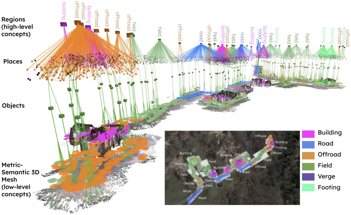
Figure 1: 3D scene graph of a indoor-outdoor environment at West Point, NY, constructed using our approach. The hierarchical structure of the graph is based on a spatial ontology generated from Large Language Models, and grounded into a 3D map using Logic Tensor Networks. A satellite image is shown of the area overlaid with the constructed 3D scene graph.

Generalizing 3D scene graphs to outdoor environments poses three main challenges: (i) Indoor vs. outdoor semantics: although there is a clear hierarchy of semantic concepts for indoor environments (e.g., objects, rooms, floors, building), the concepts needed to describe a broad variety of outdoors scenes (e.g., a rural landscape vs. a beach) is less immediate; thus, it is undesirable for a human to manually define such set of labels for each application. (ii) Lack of training datasets: while there are established training datasets one can use for indoor scene graph generation, there is virtually no dataset that allows creating semantically rich 3D scene graphs in outdoor scenes; for instance, prior work [10] leverages annotations by OpenStreetMap (OSM), but OSM only provides a handful of annotated classes (e.g., road, highway, building) and does not include smaller objects; this is problematic since existing GNN-based methods [6] train a network to group nodes (e.g., objects) into higher-level concepts (e.g., rooms) to build hierarchical representations. (iii) Reliability of learning-based methods: GNN-based approaches can provide incorrect predictions, especially when trained on relatively small datasets or tested outside the training domain; thus, an approach to constrain GNN predictions using common-sense knowledge to improve generalization and accuracy across scenes is desirable.

Contribution. We tackle the three challenges above and propose a neuro-symbolic approach to extend 3D scene graph construction to arbitrary environments. To address the first challenge, we construct a spatial ontology (Section IV) that describes spatial concepts and relations, which represents common-sense spatial knowledge (e.g., a "bathroom" contains a "shower"). While it is well-known that building a comprehensive ontology is difficult and time-consuming, we show that Large Language Models (LLM) can be used to automatically build an ontology, and we show they can produce a reasonable ontology without fine-tuning and with minimal human effort.

To address the second and third challenge, we resort to a novel learning approach, namely Logic Tensor Networks (LTNs) [11] (Section V). LTNs provide a way to add logical rules while training a neural network; these rules provide an additional supervisory signal at training time (hence reducing the amount of training data required) and constrain the network prediction at test time (hence increasing the reliability of the predictions). In particular, we design a model consisting of a GNN and a multi-layer perceptron (MLP) wrapped inside an LTN [11] that ensures the prediction of the semantic labels in the 3D scene graph satisfy the relations encoded by the spatial ontology.

We evaluate our approach in a variety of datasets, including indoor, rural, and coastal environments (Section VI). Our results show that the proposed approach enhances performance with limited training data; for instance, the LTN boosts performance from 12.3% to 25.1% for the tested indoor scenes and 29.0% to 37.2% (on average) for the tested outdoor scenes when training the proposed model using only 0.1% of the training data. Furthermore, the LTN-based approach predicts labels unseen at training time by leveraging common-sense relations between objects and the location containing them encoded by the spatial ontology.

II Related Work

3D Scene Graphs. The pioneering work of Armeni et al. [1] introduced the notion of 3D scene graphs as a hierarchical model of 3D environments. Following this, Rosinol et al. [3, 2] extended this model to construct 3D scene graphs from sensor data while adding a richer hierarchy of layers. Other representative approaches also explore constructing 3D scene graphs from geometric data via GNNs [12] or probabilistic approaches [13, 14]. More recently, several approaches explore the creation of 3D scene graphs in real-time [5, 4] or specific outdoor (i.e., urban) environments [15]. Most relevantly, Hughes et al. [6] discuss detecting higher-level concept categories (e.g., room types) in 3D scene graphs using a fully-supervised GNN approach in an online manner, and Chen et al. [16] discuss using large language models for zero-shot room classification in 3D scene graphs.

Additionally, 3D scene graphs have started to find many applications in robotics and beyond. Recent works have successfully used 3D scene graphs for navigation [9, 17] as well as task and motion planning [8, 7]. Finally, 3D scene graphs also have nascent applications outside of robotics [18, 19].

Ontologies. To build and share a meaningful representation of a 3D environment, a robot needs a common "vocabulary" describing the concepts and relations observed by the robot. Such a vocabulary may be represented as an ontology. The precise definition of ontology varies between communities [20], and the term is often used interchangeably with knowledge graph and knowledge base. Typically, an ontology refers to the “schema” of data (i.e., abstract concepts and relations) whereas a knowledge graph is an instance of an ontology populated with data. We adopt the definition of knowledge base from [11] (more details in Section V). A significant effort has been made in the creation of common-sense ontologies and knowledge graphs [21, 22] , and there has been a surge applying these to problems such as 2D scene graph generation [23], image classification [24], and visual question answering [25], to name a few. Most relevant to our work, Qiu et al. [26] and Zhang et al. [27] use ontologies to inform the generation of indoor 3D scene graphs, and Hsu et al. [28] discuss how to use LLMs to generate grounding predicates for object and their relationships. Constructing common-sense ontologies and knowledge graphs is an open problem; many authors have recently explored the role and use of LLMs to generate these representations. These works discuss either how to directly create common-sense representations by refining the LLM output [29] or evaluate the common-sense knowledge accuracy of LLMs [30]. The interested reader is referred to [31] for a discussion of challenges in this area.

III Problem Statement

A 3D scene graph (e.g., Fig. 1) is a hierarchical graph [6] where nodes and edges represent spatial concepts and relations grounded in the physical world, and are grouped into layers corresponding to different levels of abstraction of the scene. In indoor environments, the layers (from bottom to top) consist of a metric-semantic 3D mesh, objects and agents, places (a topological representation of free space), and rooms (groupings of places describing rooms). The inter-layer edges connect high-level concepts to low-level concepts. For example, a room is connected to places (representing the free space in that room), and subsequently, the places in a room are connected to vertices in the metric-semantic 3D mesh (representing the geometry of the room). While existing work on 3D scene graphs focus on grounding concepts for indoor environments, we extend the 3D scene graph model in [2, 4] to ground concepts in arbitrary environments (e.g., indoor and outdoor). Specifically, given the low-level layers (i.e., metric-semantic 3D mesh, objects and agents, and places) which have the same meaning in both indoor and outdoor environments and can be built as in [4], we construct the high-level layers (i.e., regions layer generalizing the rooms layer) of a 3D scene graph based on a given set of spatial concepts (e.g., “kitchen” and "bathroom" for indoors or “road” and “field” for outdoors).

IV Language-enabled Spatial Ontologies

This section introduces the notion of spatial ontology and describes how to generate one using LLMs.

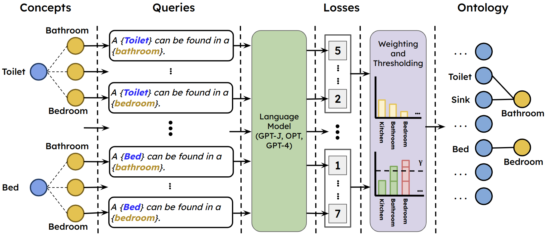
Figure 2: Text scoring approach for generating spatial ontology. The language model assigns a loss to the text string between low-level and high-level labels. The loss is rescaled using a softmax to assign weights to the edges, then the lowest weighted edges are pruned away.

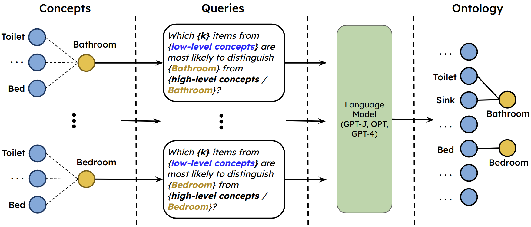
Figure 3: Text completion approach for generating spatial ontology. The language model is queried asking what low-level labels distinguish high-level labels. The response is parsed to generate the spatial ontology.

IV-A Spatial Ontology

A spatial ontology is a representation of spatial knowledge, which can be modeled as a graph where nodes are (abstract) spatial concepts and edges are spatial relations between the concepts. In this work, we consider a spatial ontology where each node corresponds to either low-level spatial concepts ${\cal L}=\{\ell_{1},\cdots,\ell_{n}\}$ or high-level spatial concepts ${\cal H}=\{h_{1},\cdots,h_{m}\}$ where the $n$ low-level and $m$ high-level concepts correspond to semantics captured by the mesh layer (e.g., sand, rock) and locations captured by the places layer (e.g., beach), respectively. Furthermore, we only consider inclusion relations, which describe where low-level concepts may be located with respect to high-level concepts. For example, an edge between a low-level concept $\ell\in{\cal L}$ (e.g., “sink”) and a high-level concept $h\in{\cal H}$ (e.g., “kitchen”) means that $\ell$ is located within $h$ (e.g., a “sink” is located in a “kitchen”). This implies that the spatial ontology is a bipartite graph with $|{\cal H}|\times|{\cal L}|$ biadjacency matrix ${\bm{\Omega}}$. In contrast to a 3D scene graph, which is a grounded representation of the environment, a spatial ontology is independent from the specific environment observed by the robot. For example, the concept of “chair” in an ontology is not associated with a particular instance of a “chair”, while in a 3D scene graph, the concept of “chair” is grounded in the scene the robot observes. In other words, an ontology is a graph representing all possible concepts and their relations (i.e., it describes that chairs are typically in kitchens), while a 3D scene graph is a model of a specific environment (i.e., an instantiation of a spatial ontology with data).

IV-B Inferring Spatial Ontologies from LLMs

While a spatial ontology may be defined manually by an expert, such manual effort is time-consuming and does not scale well to large ontologies. In this section, we describe two approaches to use LLMs to build spatial ontologies at scale.

IV-B1 Text Scoring

In this approach, we initially assume edges exist between all pairs of low-level and high-level concepts. Weights are assigned to each edge in the ontology each representing if a low-level concept is located within a high-level concept. The weights on the edges are assigned using an auto-regressive language model $\Lambda$, which is trained to assign probabilities to text strings. More precisely, $\Lambda$ maps strings of tokens $W$ to the log probability of the string written as $\Lambda(W)\approx\text{log}\,p(W)$. The template $g_{score}$ for generating the text string between the $i$th low-level concept $\ell_{i}\in{\cal L}$ and the $j$th high-level concept $h_{j}\in{\cal H}$ is given by

$$g_{score}(i,j)=\text{``}\ell_{i}\;\text{is often found in}\;h_{j}\text{''}.$$

The language model assigns a loss to each edge based on the associated text string, then the weights for each edge are rescaled using a softmax function:

$$w_{ij}=\frac{\exp\{\Lambda(g_{score}(i,j))/K\}}{\sum_{k=1}^{|H|}\exp\{\Lambda(g_{score}(i,k))/K\}},$$ (1)

where $K\in(0,\infty]$ is a temperature parameter. The weights for the edges incident to each low-level concept are accumulated in descending order by weight until exceeding a threshold $\gamma$, then the edges not reached are pruned from the spatial ontology; formally, the $r$ retained edges for the $i$th low-level concept satisfy $\sum_{j=1}^{r-1}w_{ij}\leq\gamma$ and $\sum_{j=1}^{r}w_{ij}>\gamma$ where $\gamma$ is a user-defined threshold. Figure 2 provides an overview of the overall approach.

IV-B2 Text Completion

While the approach described above generates reasonable ontologies (more in Section VI), the result is a spatial ontology with edges for the most likely relations (e.g., a “wall” is more likely to be located in a “bathroom” than a “shower”) instead of an ontology with edges that are useful for distinguishing between different high-level concepts given low-level concepts (e.g., a “shower” is more likely to distinguish a “bathroom” from a “bedroom” than a “wall”). Here, we construct the spatial ontology by querying the language model for each high-level concept to generate $k$ edges connecting low-level concepts. The template $g_{comp}$ for generating the text string for $k$ edges associated with the $i$th high-level concept $h_{i}\in{\cal H}$ is given by

$$g_{comp} (i,k)=\text{``Which }\{k\}\text{ items from }\{{\cal L}\}\text{ are most }$$

$$\text{likely to distinguish }\{h_{i}\}\text{ from }\{{\cal H}/h_{i}\}.\text{ Answer}$$

$$\text{with a python list using exact strings in }\{{\cal L}\}\text{.''}$$

After querying the language model, the response requires post-processing since the language model may incorrectly format the response or hallucinate concepts. This is resolved in practice by verifying the format and checking for hallucinated concepts (i.e., concepts not from ${\cal L}$). If the response is invalid, the formatting is corrected during post-processing, and if hallucinated concepts are returned in the response, the text string used for the query is appended with “Do not respond with concepts in $\{{\cal L}^{\prime}\}$” where ${\cal L}^{\prime}$ is a list of invalid low-level concepts generated from hallucinated concepts. Furthermore, the response generated by the language model is stochastic; thus, each query is repeated $N$ times, and the top $k$ edges generated are used in the spatial ontology; see Figure 3.

V Leveraging Spatial Ontologies
for 3D Scene Graph Generation

This section briefly reviews LTNs and shows how to generate 3D scene graphs using LTNs.

V-A Logic Tensor Networks

A Logic Tensor Network (LTN) [11] is a neuro-symbolic framework that combines explicit symbolic knowledge expressed as a set of logical formulas with implicit subsymbolic knowledge (e.g., encoded within the parameters of a neural network). LTNs support tasks such as learning (making generalization from data), reasoning (verifying a consequence from facts), and query-answering (evaluating the truth value of a logical expression). To express the relationship between symbolic and subsymbolic knowledge, LTNs are built on Real Logic [32], which is a differentiable first-order language with infinitely many truth values in $[0,1]$. This allows converting Real Logic formulas (e.g., a differentiable loss) into computational graphs that enable gradient-based optimization.

V-A1 Syntax of Real Logic

Formally, Real Logic is defined on a first-order language ${\cal F}$ with a signature consisting of sets of symbols for constants, variables, functions, and predicates. A formula (or axiom) in ${\cal F}$ is an expression constructed using symbols in the signature together with logical connectives, $\neg,\land,\lor,\rightarrow$, and quantifiers, $\forall,\exists$, following the same syntax as First-Order Logic (FOL). For example, we can construct a formula stating that “every kitchen contains a sink” as $\forall y({\normalsize\texttt{Kitchen}}(y)\rightarrow\exists x({\normalsize\texttt{Sink}}(x)\land{\normalsize\texttt{PartOf}}(x,y))$, where $x,y$ are variables and ${\normalsize\texttt{Sink}}(\cdot)$, ${\normalsize\texttt{Kitchen}}(\cdot)$, ${\normalsize\texttt{PartOf}}(\cdot,\cdot)$ are predicates. In real-world scenarios, a formula may be partially true (e.g., a kitchen may exist that does not contain a sink); thus, Real Logic adopts continuous truth values in $[0,1]$.

V-A2 Semantics of Real Logic

The semantics of Real Logic are the rules for interpreting symbols with respect to the real world, thus explicitly connecting symbolic and subsymbolic knowledge. Intuitively, interpretations ${\cal I}$ are the numeric values associated with each symbol, as well as how to numerically implement the operations applied to such values. In general, constants and variables are interpreted as tensors, whereas operations include functions, which map tensors to tensors, and predicates, which map tensors to real numbers in $[0,1]$. For example, a variable $x$ may be interpreted as a feature vector associated to an object observed by the robot (e.g., sink), and the predicate ${\normalsize\texttt{Sink}}(\cdot)$ may be interpreted as a binary classifier that takes a feature vector as input and returns if the input is a sink or not (e.g., returning a truth value between 0 and 1). In Real Logic, a formula $\phi$ under an interpretation ${\cal I}$ is satisfied if ${\cal I}(\phi)=1$, but in practice, a formula $\phi$ is typically only partially satisfied (i.e., ${\cal I}(\phi)\in[0,1]$). Since predicates are partially true or false, there are various ways of defining connectives and quantifiers (e.g., see  [33]).

V-A3 Learning with LTNs

If we are given a set of formulas in Real Logic, LTNs allow learning the interpretation of symbols in the signature. For example, if constants are interpreted as embeddings, and functions and predicates are interpreted as neural networks, the interpretation ${\cal I}$ depends on learnable parameters $\theta$ with a parametric interpretation denoted by ${\cal I}(\cdot|\theta)$. The symbols in the signature, logical formulas, and interpretations together are referred to as a Real Logic knowledge base. The optimization problem underlying LTNs for learning interpretations is a satisfiability problem, which yields the values of the parameters $\theta^{*}$ that maximize the truth values of the conjunction of a set of logical formulas ${\cal K}$ in a Real Logic knowledge base. We can write this as:

$$\theta^{*}=\operatorname*{arg\,min}_{\theta\in\Theta}\left(1-\underset{\phi\in{\cal K}}{{\normalsize\texttt{SatAgg}}}\,{\cal I}(\phi|\theta)\right)$$ (2)

where ${\normalsize\texttt{SatAgg}}:[0,1]^{*}\rightarrow[0,1]$ is an aggregating operator over all the formulas $\phi\in{\cal K}$, typically implemented numerically as a generalized mean [11]. Since Real Logic interprets expressions as real-valued tensors, LTNs associate gradients to the expressions in the knowledge base and optimizes (2) via gradient-based optimization.

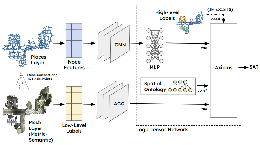
(a) Learning Phase. In the learning phase, the place features are processed by the GNN to compute node embeddings, and the MLP processes the embeddings and returns the softmax of the logits. The MLP is wrapped in an LTN to compute the satisfaction of a Real Logic knowledge base using the data-driven axioms based on ground truth labels and ontology-driven axioms based on the aggregated semantics from the mesh layer.

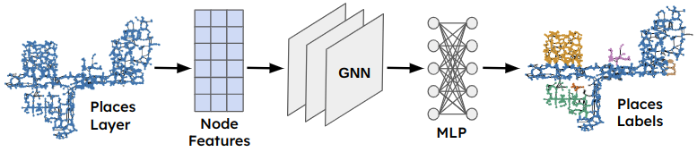
(b) Inference Phase. In the inference phase, the LTN is dropped, and the model predicts the node labels based on the place features using the trained MLP and GNN from the learning phase.

Figure 4: Proposed architecture for learning and inference.

V-B Formalizing 3D Scene Graph Generation in LTNs

This section presents our approach to create hierarchical 3D scene graphs with a spatial ontology using LTNs. Specifically, given the low-level layers of a 3D scene graph (i.e., metric-semantic 3D mesh, objects and agents, and places), we construct the high-level layers based on a given spatial ontology and labeled examples (if available). We formulate this as a node classification problem on the places layer using a GNN for generating node embeddings and an MLP for predicting node labels. We leverage LTNs during training to constrain the model to make predictions consistent with the spatial ontology. The proposed architecture for learning and inference is given in Fig. 4. We train the model end-to-end to learn the parameters of both the GNN and MLP based on the satisfaction of a knowledge base, as described below.

V-B1 Constants and Variables

While constants and variables are used in the same way in functions and predicates, the difference is that variables can appear in quantifiers (i.e., a variable can have different instances with different values while constants are always a fixed value).

Constants. The graph representing the places layer of a 3D scene graph is denoted by ${\cal G}=({\cal V},{\cal E})$ where ${\cal V}$ is the set of place nodes and ${\cal E}$ is the set of edges between place nodes. The label space is $\{y_{1},\cdots,y_{m}\}$, which corresponds to the $m$ high-level concepts ${\cal H}$ in the spatial ontology; specifically, $y_{i}$ is a constant interpreted as the one-hot vector for $h_{i}\in{\cal H}$. The spatial ontology is a constant ${\bm{\Omega}}$ interpreted as the $|{\cal H}|\times|{\cal L}|$ biadjacency matrix (e.g., built using either of the approaches described in Section IV), which defines the valid choices of a high-level concepts for a place node given the low-level concepts observed by the robot at that place node.

Variables. The GNN associates an embedding $x_{v}$ to each place node $v\in{\cal V}$. This embedding will eventually be passed to an MLP to classify the high-level concept (i.e., region) the node belongs to. At the same time, we attach a second (pre-computed) feature vector $q_{v}$ to each place node $v\in{\cal V}$, describing the low-level concepts observed by the robot at that node (e.g., nearby objects). More in detail, each place node is connected to nearby nodes in the metric-semantic 3D mesh, called basis points (as described in [6]); the semantic labels of the basis points are one-hot vectors representing the low-level concepts ${\cal L}$ in the ontology. We build $q_{v}$ as the histogram of semantic labels of the basis points connected to a node $v\in{\cal V}$.

V-B2 Predicates

The predicates take constants and variables as input and return a real number in $[0,1]$. Here, we propose predicates, which are either data-driven (referred to as equivalence predicates) or ontology-driven (referred to as inclusion predicates). This allows learning the interpretations of predicates parameterized by the parameters $\theta$ of our model using a combination of labeled data and unlabeled data. Specifically, the equivalence predicates rely only on the constants $y_{i}$ (i.e., the labeled data) while inclusion predicates rely only on the constant ${\bm{\Omega}}$ (i.e., only use the spatial ontology).

Equivalence. We propose ${\normalsize\texttt{IsClassOf}}(\cdot,\cdot|\theta)$ as an equivalence predicate, which quantifies if a high-level concept predicted by the ${\normalsize\texttt{MLP}}_{\theta}(\cdot)$ for a place node matches the ground truth label (if available at training time):

$${\cal I}({\normalsize\texttt{IsClassOf}}|\theta):x_{v}^{(i)},y_{i}\mapsto y_{i}^{T}\cdot{\normalsize\texttt{MLP}}_{\theta}(x_{v}^{(i)})\;\;$$ (3)

where $x_{v}^{(i)}$ denotes the embedding for a place node $v\in{\cal V}$ with label $y_{i}$. In words, the predicate measures the agreement between the predicted label ${\normalsize\texttt{MLP}}_{\theta}(x_{v}^{(i)})$ and the ground truth label $y_{i}$, and represents the statement: “A place node with label $y_{i}$ is classified as $y_{i}$”. Intuitively, this predicate plays a similar role as cross-entropy loss in standard supervised learning.

Inclusion. At training time, we encourage the model (i.e., GNN+MLP) to predict labels for place nodes that match the spatial ontology based on the connected basis points. More formally, we build a formula stating “If the spatial ontology has connections valid with the basis points connected to a place node, the place node is classified with a label similar to the ones encoded in the spatial ontology”. The first part of the formula is to circumvent missing data in the spatial ontology: for instance, the ontology may have disconnected low-level concepts, and we do not use the ontology in those cases. The second part encourages the prediction to agree with at least one of the edges in the spatial ontology. In order to formalize this formula, we need two predicates: ${\normalsize\texttt{IsValid}}(\cdot,\cdot)$ and ${\normalsize\texttt{IsSimilar}}(\cdot,\cdot,\cdot|\theta)$, which we describe below.

In order to assert the validity of the low-level concepts $q_{v}$ attached to a node $v\in{\cal V}$ (i.e., that low-level concepts connected to a place node are connected to high-level concepts in the ontology), we define a predicate ${\normalsize\texttt{IsValid}}(\cdot,\cdot)$:

$${\cal I}({\normalsize\texttt{IsValid}}):{\bm{\Omega}},q_{v}\mapsto{\normalsize\texttt{sum}}(\hat{{\bm{\Omega}}}\cdot\hat{q_{v}})$$ (4)

where $\hat{\cdot}$ is an operator normalizing columns with respect to the $\ell_{1}$-norm. Intuitively, ${\normalsize\texttt{IsValid}}({\bm{\Omega}},q_{v})=0$ if none of the low-level concepts in the histogram $q_{v}$ are connected to a high-level concept in the spatial ontology ${\bm{\Omega}}$.

Next, we define the predicate ${\normalsize\texttt{IsSimilar}}(\cdot,\cdot,\cdot|\theta)$ to quantify the degree that high-level concepts predicted by the MLP are similar to the expected high-level concepts in the spatial ontology based on the low-level features $q_{v}$:

$${\cal I}({\normalsize\texttt{IsSimilar}}|\theta):x_{v},{\bm{\Omega}},q_{v}\mapsto{\normalsize\texttt{MLP}}_{\theta}(x_{v})^{T}\cdot\hat{{\bm{\Omega}}}\cdot\hat{q_{v}}.$$ (5)

Intuitively, $\hat{{\bm{\Omega}}}\cdot\hat{q_{v}}$ represents the valid high-level concepts associated to low-level concepts in $q_{v}$ (according to the ontology ${\bm{\Omega}}$), and the predicate computes the similarity between these high-level concepts and the ones predicted by the model, which enforces alignment between the model predictions ${\normalsize\texttt{MLP}}_{\theta}(x_{v})$ and ontology predictions $\hat{{\bm{\Omega}}}\cdot\hat{q_{v}}$ .

V-B3 Axioms

The axioms are the logical formulas constructed from constants, variables, and predicates representing statements. We distinguish the axioms by whether they use the equivalence or the inclusion predicates. The equivalence axioms $\phi_{\text{Equiv}}$ and inclusion axioms $\phi_{\text{Incl}}$ are:

$$\phi_{\text{Equiv}}\!: \;\forall x_{v}^{(i)}\;{\normalsize\texttt{IsClassOf}}(x_{v}^{(i)},y_{i})$$

$$\phi_{\text{Incl}}\!: \;\forall x_{v},q_{v}\;{\normalsize\texttt{IsValid}}({\bm{\Omega}},q_{v})\!\rightarrow{\normalsize\texttt{IsSimilar}}(x_{v},{\bm{\Omega}},q_{v})$$

where diagonal quantification is used for both $\phi_{\text{Equiv}}$ and $\phi_{\text{Incl}}$ as described in [11]. Here, $x_{v}^{(i)}$ corresponds to place nodes with label $y_{i}$, and each place node $v\in{\cal V}$ is assigned features $x_{v}$ and $q_{v}$; thus, we only want to construct statements between $x_{v}$ and $q_{v}$ for each $v\in{\cal V}$. At training time, the equivalence axioms promote the model to make predictions that agree with the annotated labels (if available), while the inclusion axioms encourage the model to make prediction that agree with the spatial ontology based on the semantics of the connected basis points.

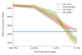
(a) MP3D

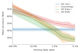
(b) West Point

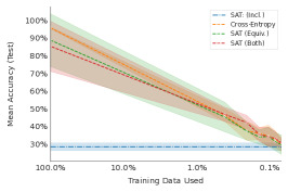
(c) Castle Island

Figure 5: (a) Results of the predicate ablation for the MP3D dataset. (b) Results of the predicate ablation for the West Point dataset. (c) Results of the predicate ablation for the Castle Island dataset. For all experiments, we run 10 trials of each loss configuration for each percentage of the training data. The mean of the 10 trials is shown as a dashed line, and the shaded area shows the standard deviation.

VI Experiments

VI-A Experimental Setup

We utilize three datasets for our experiments: Matterport3D (MP3D) [34], West Point, and Castle Island. For all datasets, we use Hydra [6] to generate 3D scene graphs.

MP3D. The MP3D [34] dataset is an RGB-D dataset consisting of 90 indoor scenes. We use the Habitat simulator [35] to render the visual and human-annotated semantic data for the scenes. The provided label space has 40 semantic labels (i.e., mpcat40 [34]), of which we discard the labels gym_equipment and beam. For our experiments, we use the official train, test, and validation splits of the scenes [34].

West Point and Castle Island. We collect two outdoor datasets. The first of these datasets, West Point, consists of two robot trajectories where a RealSense D455 was mounted on a Clearpath Jackal rover. These trajectories explore areas mostly consisting of roads, fields, and buildings. The second dataset, Castle Island, was collected from Pleasure Bay beach in Boston via a hand-held sensor payload, which consists of two trajectories. The trajectories explore areas around the beach and nearby parking lot. The trajectories from both datasets are roughly a half kilometer to a kilometer in length. For both datasets, we use OneFormer [36] to provide semantics (i.e., low-level concepts) with the ADE20k [37] label space. We use LOCUS [38] with a Velodyne mounted on the Jackal to provide trajectory estimates for the West Point dataset, and Kimera-VIO [39] for trajectory estimates of Castle Island.

Training. We train the model using different axiom configurations that include (i) only the data-driven axioms $\phi_{Equiv}$ (label: “SAT (Equiv.)”), (ii) only the ontology-driven axioms $\phi_{Incl}$ (label: “SAT (Incl.)”), and (iii) both the data-driven and ontology-driven axioms (label: “SAT (Both)”). As a baseline, we train a GNN using cross-entropy loss (label: “Cross-Entropy”), which is expected to be roughly equivalent to the model trained with the purely data-driven axioms. The node features for the places are the concatenation of the position and the word2vec [40] encoding of the aggregated semantic labels of the child nodes in the mesh layer. For the GNN, we use a graph attention network (GAT) [41] and tune the hyper-parameters using grid search.

For the connectives and quantifiers, we use a product configuration except for the implication operator where the Goguen operator is used instead of the Reichenbach operator [33]. We use stochastic gradient descent with the Adam optimizer, and we run the optimization until the loss has converged (e.g., changes less than 1e-06 for 10 epochs) or 1000 epochs is reached. After each epoch, the model with the best validation accuracy is retained for testing. Each model is trained 10 times using a random initialization of the model parameters, and the statistics are reported in the results. We implement the learning architectures using PyTorch Geometric [42] and LTNTorch [11].

VI-B Results

We conduct an ablation study comparing the cross-entropy baseline and the different axioms configurations for the LTN. The accuracy results (i.e., percentage of correctly classified places) for all datasets are reported in Fig. 5. For each dataset, we evaluate the performance for $100\%$, $10\%$, $1\%$, $0.4\%$, $0.2\%$, and $0.1\%$ of the training data. As mentioned, we use the train-test-validation splits for MP3D as described in [34], and we mask these percentages of place nodes from the training scene to simulate a scenario where annotated data is limited. For West Point and Castle Island, we instead train in a semi-supervised manner where we combine both graphs ($70\%$ for training and $15\%$ for validation and testing), as the datasets are too small to generalize from a single training scene to a single testing scene.

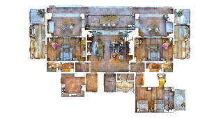
(a) MP3D Mesh

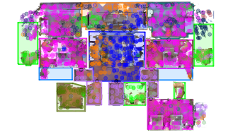
(b) MP3D

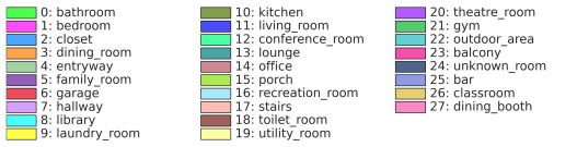
(c) MP3D Color Legend

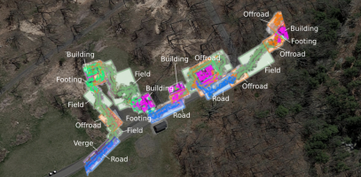
(d) West Point

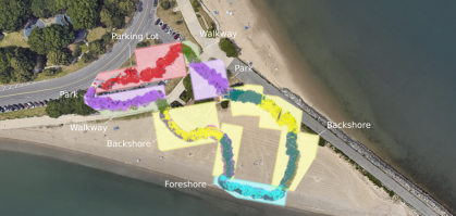
(e) Castle Island

(f) Outdoor Color Legend

Figure 6: (a) The “q9vSo1VnCiC” scene from MP3D and (b) classified place nodes for the “q9vSo1VnCiC” scene along with (c) associated color legend for node labels. (d) Classified place nodes for one of the West Point trajectories. (e) Classified place nodes for on of the Castle Island trajectories. (f) Associated color legend for both West Point and Castle Island. The ground truth regions are drawn as shaded polygons, while the place nodes are all drawn as circles.

The data-driven approaches (our approach, the GNN baseline, and our data-driven axiom variant) show similar performance when trained on the full MP3D test dataset; see Fig. 5a. However, as less data is used during training, the purely data-driven approaches tend towards performance comparable with randomly guessing labels, while the proposed approach does not fall below the performance of the purely ontology-driven approach. The same trend is visible in Fig. 5b for the West Point dataset. The data-driven approaches in Fig. 5c for the Castle Island dataset do not have a significant gap in performance compared to the ontology-driven approaches. This is due to a lack in distinguishing low-level concepts for the high-level concepts in the scene.

Ontology	MP3D	West Point	Castle Island
$k=1$	$14.0\pm 2.0$	$37.8\pm 0.3$	$16.1\pm 3.6$
$k=2$	$16.7\pm 3.6$	$11.9\pm 14.7$	$\mathbf{28.7}\pm\mathbf{2.2}$
$k=3$	$23.1\pm 0.2$	$\mathbf{42.7}\pm\mathbf{0.2}$	$24.5\pm 0.6$
$k=4$	$2.7\pm 0.0$	$39.9\pm 4.7$	$28.7\pm 8.5$
$k=5$	$12.3\pm 0.0$	$38.8\pm 12.0$	$19.7\pm 7.1$
Custom	$\mathbf{27.7}\pm\mathbf{0.4}$	$27.7\pm 1.3$	$22.7\pm 1.8$

TABLE I: Comparison of mean accuracy achieved by the “SAT (Incl.)” loss configuration across the three datasets between the LLM generated ontologies ($k=1,\ldots,5$) versus a hand-generated ontology for the same low-level label space and high-level concepts. Best in bold.

For the ontology-driven models, we use the text completion mentioned in Section IV-B2 for generating the spatial ontology, which performs better than text scoring mentioned in Section IV-B1. We choose $k$ by generating ontologies with multiple values ($k{=}\{1,2,3,4,5\}$), and the $k$ with the highest test accuracy is used in the ablations. We compare these generated ontologies with a hand-generated ontology and report the results in Table I.

Finally, a 3D scene graph obtained by our method for each dataset is shown in Fig. 6. In general, the high-level concepts generated by our approach are plausible for the associated scenes. For certain scenes, our approach struggles to distinguish similar high-level concepts. This is apparent for the beach (e.g., ground truth labels “backshore” are classified as “beach” instead). Additionally, low-level concepts that contradict the spatial ontology cause our model to misclassify certain regions. This is clear in the MP3D scene shown in Fig. 6b; the lounge in the top-right of the building is misclassified as a bedroom due to the presence of a day-bed in the room, which is labeled as “bed” in the ground truth semantics of the MP3D dataset.

	% of Data Kept for MP3D w/ Partial Labels
Loss	100%	0.4%	0.2%	0.1%
CrossEntropy	$24.1\pm 2.4$	$16.7\pm 5.6$	$12.7\pm 4.7$	$12.5\pm 5.1$
SAT (Equiv.)	$24.7\pm 1.4$	$15.8\pm 4.0$	$12.8\pm 5.5$	$11.7\pm 5.1$
SAT (Incl.)	$22.7\pm 0.6$	$\mathbf{22.7}\pm\mathbf{0.6}$	$22.7\pm 0.6$	$22.7\pm 0.6$
SAT (Both)	$\mathbf{32.5}\pm\mathbf{1.2}$	$20.6\pm 1.4$	$\mathbf{22.8}\pm\mathbf{1.9}$	$\mathbf{23.3}\pm\mathbf{1.4}$

TABLE II: Accuracy for different holdout percentages of training data with labels masked for bathroom, kitchen, hallway, bedroom, living room, and family room. No data held out during testing. Best in bold.

Lastly, we show in the MP3D dataset that the ontology-driven models allow predicting labels unseen at training time. This scenario is simulated by masking all place nodes for a particular set of labels. Here, we mask the place nodes with labels bathroom, kitchen, hallway, bedroom, living room, and family room. In this scenario, the ontology-driven models significantly outperform the purely data-drive models as shown in Table II since labels for the removed classes are missing during training.

VII Conclusion

We propose the first approach to build hierarchical 3D scene graphs of arbitrary (indoor and outdoor) environments. Towards this goal, we leverage Large Language Models to build a spatial ontology that defines the set of concepts and relations relevant for robot operation. We show how to use such a spatial ontology for 3D scene graph construction using Logic Tensor Networks (LTN), which allow adding logical rules, or axioms (e.g., “a beach contains sand”), during training and prediction. We test our approach in a variety of datasets, including indoor, rural, and coastal environments, and show that it leads to a significant increase in the quality of the 3D scene graph generation with sparsely annotated data, and it produces reasonable results even in a zero-shot setting.

-A Details for Training

Here, we provide additional details on training the proposed model.

Implementation. We implement the learning architectures using PyTorch Geometric [42] version 2.3.1 built with CUDA verion 11.7 and LTNTorch [11] version 1.0.1, and we use GPT-4 for generating the spatial ontology. For the GNN, we use GAT [41] for the message passing layers, and we use ReLU activation functions and dropout between message passing layers where dropout is enabled for training but disabled for testing. After the messaging passing layers in the GNN, the hidden states are passed to the MLP with a linear layer followed by ReLU activation functions followed by another linear layer, then a softmax layer is applied for predicting the node labels. The input and hidden dimensions for the MLP are the same as the hidden dimensions for the message passing layers in the GNN.

Hyper-Parameter Tuning. We provide details on the method applied to tune the hyper-parameters of our model. Specifically, we search over the following sets:

• Message passing iterations: $[1,2,3]$

• Message passing hidden dimensions: $[16,32,64]$

• Number of attention heads: $[1,2,4]$

• Learning rate: $[0.01,0.001,0.0001]$

• Dropout probability: $[0.1,0.25,0.5]$

• Weight decay: $[0.005,0.0005,0.00005]$

In order to provide fair comparison between the different axioms configurations, a grid search was performed over these hyper-parameters for the Cross-Entropy configuration as well as each of the LTN configurations. For the Cross-Entropy configuration and the LTN configurations, the number of convolutional layers, the learning rate, and the weight decay made the most impact on the accuracy of the model (with weight decay making less impact than convolutional layers and learning rate). Thus, we tune the hyper-parameters for the message passing iterations while keeping the remaining parameters constant at the median values. The learning rate and weight decay are next tuned by searching over all combinations of these values, and the grid search is performed over the dropout rate and the number of attention heads. The grid search described above was performed with $1000$ epochs using the MP3D dataset, and we repeated this process for the learning rate and weight decay for both the West Point and Castle Island datasets, and optimal values of hyper-parameters remained the same as for the MP3D dataset. The optimal hyper-parameters based on the grid search are the same for each of the Cross-Entropy and different axioms configuration; see Table III for the selected values of the hyper-parameters.

Layers	3
Hidden Dimension	32
Learning Rate	0.001
Dropout	0.25
$L_{2}$ Regularization	5e-05
Attention Heads	4

TABLE III: Hyper-parameters for training the proposed model where the same hyper-parameters are used for the Cross-Entropy configuration and the LTN configurations.

Additionally, we must select the fuzzy logical operators used for the axioms in the LTN along with the hyper-parameters associated with these operators. For the implication operator, we use the Goguen operator instead of the more commonly used Reichenbach operator, as the Goguen operator provided better accuracy. Additionally, we use the $p$-mean error for the aggregating operator ${\normalsize\texttt{SatAgg}}(\cdot)$ as described in [11], and we use $p{=}2$ for the data-driven axioms (i.e., equivalence axioms) and $p{=}4$ for the ontology-driven axioms (i.e., inclusive axioms). The model was trained with $p=[2,4]$ for each axiom configuration, and the optimal value was selected; however, the difference in accuracy was insignificant.

Additionally, for the experiments where only a percentage of annotations for the data is kept during training, the annotations kept are selected randomly; furthermore, we seed the random number generator identically between the experiments for the Cross-Entropy configuration and the different LTN configurations, so the results are consistent and reproducible between experiments. Furthermore, we use a different seed for each of the Monte-Carlo trials in the experiments (e.g., trial $1$ is seeded as $1$, trial $2$ is seeded as $2$, and so on for the Cross-Entropy and LTN configurations).

Runtime. The model is trained using an AMD Ryzen Threadripper PRO 5955WX for the CPU and an NVIDIA GeForce RTX 4090 for the GPU. The runtime for training and testing the proposed model is provided in Table IV. Note, the number of parameters of the model does not change between the Cross-Entropy and LTN configurations; thus, the runtime during testing is not affected by the configuration used during training.

Loss	MP3D	West Point	Castle Island
Cross-Entropy	$0.018$s	$0.002$s	$0.005$s
SAT (Equiv.)	$0.035$s	$0.003$s	$0.007$s
SAT (Incl.)	$0.027$s	$0.003$s	$0.006$s
SAT (Both.)	$0.038$s	$0.003$s	$0.008$s
Testing (CPU):	$0.027s$	$0.067$s	$0.207$s

TABLE IV: Comparison of runtime for the proposed model for training and testing. The reported time is averaged across all epochs and all graphs for training and across all graphs for testing. The average number of (nodes, edges) for the graphs in each dataset are $(1283,7407)$ for MP3D, $(3930,15057)$ for West Point, and $(11059,69784)$ for Castle Island.

-B Evaluation of Spatial Ontology

Here, we provide an evaluation of the generated ontologies using the proposed methods for text scoring and text completion against a ground truth ontology based on human judgement. Specifically, we annotated a random sample of relations between low-level and high-level concepts (e.g., a "sink" is found in a "kitchen") as being "likely", "sometimes", and "rarely". We sample 38 pairs where an edge exists between 22 of the pairs (annotated as "likely") and an edge does not exist between 16 of the pairs (annotated as "sometimes" or "rarely"). Next, we compute the accuracy, precision, and recall for the spatial ontologies generated by the text scoring approach (using a temperature of $K=10$) and the text completion approach (using $k=\{1,2,3,4,5\}$) against the human annotated relations; see Table V. For the MP3D dataset, there are 31 high-level and 39 low-level concepts, and for the outdoor datasets, there are 15 high-level and 150 low-level concepts. For the text completion approach, the number of edges is $k|{\cal H}|$, which is $78$ ($k=3$) for MP3D, $42$ for West Point ($k=3$), and $28$ for Castle Island ($k=2$). Note, we do not include rooms labeled unknown when generating the spatial ontology. The number of edges is 99 for the MP3D dataset using the text scoring approach, and the text scoring approach was not applied to the outdoor datasets.

Ontology	Accuracy	Precision	Recall
Text Completion ($k{=}1$)	$0.50$	$\mathbf{1.0}$	$0.14$
Text Completion ($k{=}2$)	$0.52$	$0.83$	$0.22$
Text Completion ($k{=}3$)	$0.65$	$\mathbf{1.0}$	$0.40$
Text Completion ($k{=}4$)	$0.68$	$0.85$	$0.54$
Text Completion ($k{=}5$)	$0.71$	$0.86$	$0.59$
Text Scoring	$\mathbf{0.81}$	$0.77$	$\mathbf{0.95}$

TABLE V: Evaluation of indoor spatial ontologies generated using the methods for text scoring and text completion based on ground truth ontologies based on human judgement. Best in bold.

While the accuracy and recall for the text scoring approach significantly outperforms the text completion approach, the precision is significantly better for the text completion approach. Since the ontology is generally sparse, the precision of the spatial ontology is a better performance indicator for the LTN, which is consistent with the results. Recall, the value of $k{=}3$ provides the best accuracy for the LTN for the MP3D dataset as shown in Table I, which is also the spatial ontology tied with $k{=}1$ for the highest precision (where $k{=}3$ has higher accuracy and recall than $k{=}1$). Furthermore, this can be observed by comparing the accuracy for grounding the high-level concepts in 3D scene graphs using the text completion versus the text scoring approaches; see Table VI.

In contrast to the text scoring approach, the text completion approach requires choosing a value of $k$, which restricts the number of edges incident to each low-level concept. The number of edges incident to each low-level concept in the text scoring approach varies between low-level concepts, which could be preferrable; however, many incident edges to a particular low-level concept indicates the concept may not be useful for distinguishing high-level concepts (e.g., "wall" is common to most rooms in a building making it a poor indicator for a room type).

	SAT (Incl.)		SAT (Both)
% Kept	Text Scoring	Text Completion	Text Scoring	Text Completion
100%	$12.1\pm 4.6$	$\mathbf{23.1}\pm\mathbf{0.2}$	$52.7\pm 4.6$	$\mathbf{52.9}\pm\mathbf{1.8}$
10%	$12.1\pm 4.6$	$\mathbf{23.1}\pm\mathbf{0.2}$	$50.7\pm 1.6$	$\mathbf{53.2}\pm\mathbf{1.1}$
1%	$12.1\pm 4.6$	$\mathbf{23.1}\pm\mathbf{0.2}$	$27.3\pm 2.4$	$\mathbf{35.9}\pm\mathbf{3.3}$
0.4%	$12.1\pm 4.6$	$\mathbf{23.1}\pm\mathbf{0.2}$	$19.8\pm 2.8$	$\mathbf{29.8}\pm\mathbf{3.2}$
0.2%	$12.1\pm 4.6$	$\mathbf{23.1}\pm\mathbf{0.2}$	$18.0\pm 1.1$	$\mathbf{26.8}\pm\mathbf{2.3}$
0.1%	$12.1\pm 4.6$	$\mathbf{23.1}\pm\mathbf{0.2}$	$16.7\pm 1.0$	$\mathbf{25.1}\pm\mathbf{2.2}$

TABLE VI: Comparison of accuracy of the proposed model between the "text scoring" and "text completion" methods for generating the spatial ontology for different percentages of data kept during training. Note, the predicates for SAT (Incl.) do not use labeled data; thus, the performance is identical across data kept during training. No data held out during testing. Best in bold.

References

- [1] I. Armeni, Z. He, J. Gwak, A. Zamir, M. Fischer, J. Malik, and S. Savarese, “3D scene graph: A structure for unified semantics, 3D space, and camera,” in Intl. Conf. on Computer Vision (ICCV), 2019, pp. 5664–5673.
- [2] A. Rosinol, A. Violette, M. Abate, N. Hughes, Y. Chang, J. Shi, A. Gupta, and L. Carlone, “Kimera: from SLAM to spatial perception with 3D dynamic scene graphs,” Intl. J. of Robotics Research, vol. 40, no. 12–14, pp. 1510–1546, 2021.
- [3] A. Rosinol, A. Gupta, M. Abate, J. Shi, and L. Carlone, “3D dynamic scene graphs: Actionable spatial perception with places, objects, and humans,” in Robotics: Science and Systems (RSS), 2020.
- [4] N. Hughes, Y. Chang, and L. Carlone, “Hydra: a real-time spatial perception engine for 3D scene graph construction and optimization,” in Robotics: Science and Systems (RSS), 2022.
- [5] S. Wu, J. Wald, K. Tateno, N. Navab, and F. Tombari, “SceneGraphFusion: Incremental 3D scene graph prediction from RGB-D sequences,” in IEEE Conf. on Computer Vision and Pattern Recognition (CVPR), 2021.
- [6] N. Hughes, Y. Chang, S. Hu, R. Talak, R. Abdulhai, J. Strader, and L. Carlone, “Foundations of spatial perception for robotics: Hierarchical representations and real-time systems,” arXiv preprint: 2305.07154, 2023.
- [7] C. Agia, K. M. Jatavallabhula, M. Khodeir, O. Miksik, V. Vineet, M. Mukadam, L. Paull, and F. Shkurti, “Taskography: Evaluating robot task planning over large 3D scene graphs,” in Conference on Robot Learning (CoRL). PMLR, Jan. 2022, pp. 46–58.
- [8] K. Rana, J. Haviland, S. Garg, J. Abou-Chakra, I. Reid, and N. Suenderhauf, “SayPlan: Grounding large language models using 3d scene graphs for scalable task planning,” in 7th Annual Conference on Robot Learning, 2023.
- [9] Z. Ravichandran, L. Peng, N. Hughes, J. Griffith, and L. Carlone, “Hierarchical representations and explicit memory: Learning effective navigation policies on 3D scene graphs using graph neural networks,” in IEEE Intl. Conf. on Robotics and Automation (ICRA), 2022.
- [10] M. Berg, G. Konidaris, and S. Tellex, “Using Language to Generate State Abstractions for Long-Range Planning in Outdoor Environments,” in IEEE Intl. Conf. on Robotics and Automation (ICRA), May 2022, pp. 1888–1895.
- [11] S. Badreddine, A. d’Avila Garcez, L. Serafini, and M. Spranger, “Logic tensor networks,” Artificial Intelligence, vol. 303, p. 103649, 2022.
- [12] J. Wald, H. Dhamo, N. Navab, and F. Tombari, “Learning 3D semantic scene graphs from 3D indoor reconstructions,” in Proceedings of the IEEE/CVF Conference on Computer Vision and Pattern Recognition, 2020, pp. 3961–3970.
- [13] N. Gothoskar, M. Cusumano-Towner, B. Zinberg, M. Ghavamizadeh, F. Pollok, A. Garrett, J. Tenenbaum, D. Gutfreund, and V. Mansinghka, “3DP3: 3D scene perception via probabilistic programming,” in ArXiv preprint: 2111.00312, 2021.
- [14] G. Izatt and R. Tedrake, “Scene understanding and distribution modeling with mixed-integer scene parsing,” in technical report (under review), 2021.
- [15] E. Greve, M. Büchner, N. Vödisch, W. Burgard, and A. Valada, “Collaborative dynamic 3d scene graphs for automated driving,” arXiv preprint arXiv:2309.06635, 2023.
- [16] W. Chen, S. Hu, R. Talak, and L. Carlone, “Leveraging large language models for robot 3D scene understanding,” arXiv preprint: 2209.05629, 2022.
- [17] Z. Seymour, N. Chowdhury Mithun, H.-P. Chiu, S. Samarasekera, and R. Kumar, “Graphmapper: Efficient visual navigation by scene graph generation,” in 2022 26th International Conference on Pattern Recognition (ICPR), 2022, pp. 4146–4153.
- [18] H. Dhamo, F. Manhardt, N. Navab, and F. Tombari, “Graph-to-3d: End-to-end generation and manipulation of 3d scenes using scene graphs,” in Proceedings of the IEEE/CVF International Conference on Computer Vision (ICCV), October 2021, pp. 16 352–16 361.
- [19] T. Tahara, T. Seno, G. Narita, and T. Ishikawa, “Retargetable ar: Context-aware augmented reality in indoor scenes based on 3d scene graph,” in 2020 IEEE International Symposium on Mixed and Augmented Reality Adjunct (ISMAR-Adjunct), 2020, pp. 249–255.
- [20] T. R. Gruber, “Toward principles for the design of ontologies used for knowledge sharing?” International journal of human-computer studies, vol. 43, no. 5-6, pp. 907–928, 1995.
- [21] S. Auer, C. Bizer, G. Kobilarov, J. Lehmann, R. Cyganiak, and Z. Ives, “DBpedia: A nucleus for a web of open data,” in Semantic Web. Springer, 2007, pp. 722–735.
- [22] R. Speer, J. Chin, and C. Havasi, “ConceptNet 5.5: an open multilingual graph of general knowledge,” in Proceedings of the Thirty-First AAAI Conference on Artificial Intelligence, ser. AAAI’17. AAAI Press, 2017, p. 4444–4451.
- [23] A. Zareian, S. Karaman, and S.-F. Chang, “Bridging knowledge graphs to generate scene graphs,” in European Conf. on Computer Vision (ECCV). Springer, 2020, pp. 606–623.
- [24] Y. Movshovitz-Attias, Q. Yu, M. C. Stumpe, V. Shet, S. Arnoud, and L. Yatziv, “Ontological supervision for fine grained classification of street view storefronts,” in IEEE Conf. on Computer Vision and Pattern Recognition (CVPR), 2015, pp. 1693–1702.
- [25] W. Zheng, L. Yin, X. Chen, Z. Ma, S. Liu, and B. Yang, “Knowledge base graph embedding module design for visual question answering model,” Pattern Recognition, vol. 120, p. 108153, 2021.
- [26] Y. Qiu and H. I. Christensen, “3d scene graph prediction on point clouds using knowledge graphs,” arXiv preprint arXiv:2308.06719, 2023.
- [27] S. Zhang, S. Li, A. Hao, and H. Qin, “Knowledge-inspired 3d scene graph prediction in point cloud,” in Advances in Neural Information Processing Systems, M. Ranzato, A. Beygelzimer, Y. Dauphin, P. Liang, and J. W. Vaughan, Eds., vol. 34. Curran Associates, Inc., 2021, pp. 18 620–18 632.
- [28] J. Hsu, J. Mao, and J. Wu, “Ns3d: Neuro-symbolic grounding of 3d objects and relations,” in Proceedings of the IEEE/CVF Conference on Computer Vision and Pattern Recognition (CVPR), June 2023, pp. 2614–2623.
- [29] C. Chen, K. Lin, and D. Klein, “Constructing taxonomies from pretrained language models,” in Proceedings of the 2021 Conference of the North American Chapter of the Association for Computational Linguistics: Human Language Technologies, 2021, pp. 4687–4700.
- [30] K. Sun, Y. E. Xu, H. Zha, Y. Liu, and X. L. Dong, “Head-to-tail: How knowledgeable are large language models (llm)? aka will llms replace knowledge graphs?” arXiv preprint arXiv:2308.10168, 2023.
- [31] J. Z. Pan, S. Razniewski, J.-C. Kalo, S. Singhania, J. Chen, S. Dietze, H. Jabeen, J. Omeliyanenko, W. Zhang, M. Lissandrini et al., “Large language models and knowledge graphs: Opportunities and challenges,” arXiv preprint arXiv:2308.06374, 2023.
- [32] R. Fagin, R. Riegel, and A. Gray, “Foundations of reasoning with uncertainty via real-valued logics,” arXiv preprint arXiv:2008.02429, 2020.
- [33] E. van Krieken, E. Acar, and F. van Harmelen, “Analyzing differentiable fuzzy logic operators,” Artificial Intelligence, vol. 302, p. 103602, 2022.
- [34] A. Chang, A. Dai, T. Funkhouser, M. Halber, M. Niessner, M. Savva, S. Song, A. Zeng, and Y. Zhang, “Matterport3d: Learning from rgb-d data in indoor environments,” International Conference on 3D Vision (3DV), 2017.
- [35] M. Savva, A. Kadian, O. Maksymets, Y. Zhao, E. Wijmans, B. Jain, J. Straub, J. Liu, V. Koltun, J. Malik, D. Parikh, and D. Batra, “Habitat: A Platform for Embodied AI Research,” in Proceedings of the IEEE/CVF International Conference on Computer Vision (ICCV), 2019.
- [36] J. Jain, J. Li, M. Chiu, A. Hassani, N. Orlov, and H. Shi, “OneFormer: One Transformer to Rule Universal Image Segmentation,” in IEEE Conf. on Computer Vision and Pattern Recognition (CVPR), 2023.
- [37] B. Zhou, H. Zhao, X. Puig, S. Fidler, A. Barriuso, and A. Torralba, “Scene parsing through ade20k dataset,” in Proceedings of the IEEE Conference on Computer Vision and Pattern Recognition, 2017.
- [38] A. Reinke, M. Palieri, B. Morrell, Y. Chang, K. Ebadi, L. Carlone, and A. Agha-mohammadi, “LOCUS 2.0: Robust and computationally efficient lidar odometry for real-time underground 3D mapping,” vol. 7, no. 4, pp. 9043–9050, 2022.
- [39] A. Rosinol, M. Abate, Y. Chang, and L. Carlone, “Kimera: an open-source library for real-time metric-semantic localization and mapping,” in IEEE Intl. Conf. on Robotics and Automation (ICRA), 2020.
- [40] T. Mikolov, K. Chen, G. Corrado, and J. Dean, “Efficient estimation of word representations in vector space,” arXiv preprints arXiv:1301.3781, 2013.
- [41] P. Veličković, G. Cucurull, A. Casanova, A. Romero, P. Lió, and Y. Bengio, “Graph attention networks,” in Intl. Conf. on Learning Representations (ICLR), May 2018.
- [42] M. Fey and J. E. Lenssen, “Fast graph representation learning with PyTorch Geometric,” in Intl. Conf. on Learning Representations (ICLR) Workshop on Representation Learning on Graphs and Manifolds, 2019.