A Simple and Practical Method for Reducing
the Disparate Impact of Differential Privacy

Abstract

Differentially private (DP) mechanisms have been deployed in a variety of high-impact social settings (perhaps most notably by the U.S. Census). Since all DP mechanisms involve adding noise to results of statistical queries, they are expected to impact our ability to accurately analyze and learn from data, in effect trading off privacy with utility. Alarmingly, the impact of DP on utility can vary significantly among different sub-populations. A simple way to reduce this disparity is with stratification. First compute an independent private estimate for each group in the data set (which may be the intersection of several protected classes), then, to compute estimates of global statistics, appropriately recombine these group estimates. Our main observation is that naive stratification often yields high-accuracy estimates of population-level statistics, without the need for additional privacy budget. We support this observation theoretically and empirically. Our theoretical results center on the private mean estimation problem, while our empirical results center on extensive experiments on private data synthesis to demonstrate the effectiveness of stratification on a variety of private mechanisms. Overall, we argue that this straightforward approach provides a strong baseline against which future work on reducing utility disparities of DP mechanisms should be compared.

Introduction

Two moral and legal imperatives, data privacy and algorithmic equity, have received significant recent research attention. For ensuring data privacy, differential privacy (DP) has emerged as a gold standard technique (Dwork, Roth et al. 2014). Academics and practitioners alike use DP algorithms to solve problems with sensitive data; notably, big tech companies like Google, Microsoft and Apple rely on differential privacy for protecting customer data (Erlingsson, Pihur, and Korolova 2014; Ding, Kulkarni, and Yekhanin 2017; Cormode et al. 2018). One recent high-profile use of DP was in the 2020 United States Census, which includes statistical disclosures with data for millions of Americans (Bureau 2021; Christ, Radway, and Bellovin 2022; Groshen and Goroff 2022; Hawes 2020). Additionally, a wide variety of popular algorithms have DP versions, from fundamental statistical methods (Dwork, Roth et al. 2014), to machine learning (Ji, Lipton, and Elkan 2014) and even deep learning (Abadi et al. 2016) techniques.

However, DP can be in tension with algorithmic equity, where, unlike for privacy, there is no “gold standard” definition, and where potential harms are murky and plentiful (Corbett-Davies and Goel 2018; Mitchell et al. 2021). The 2020 Census, for example, was criticized over concerns that DP techniques would have adverse impacts on estimating demographic proportions (Ruggles et al. 2019) and on redistricting (Kenny et al. 2021). In fact, much attention has been paid lately to disparities in performance of DP mechanisms in a variety of settings, and to potential harms resulting from such disparities (Fioretto et al. 2022). Many of these works demonstrate disparities in performance for different demographic groups within the data (Bagdasaryan, Poursaeed, and Shmatikov 2019; Ganev, Oprisanu, and De Cristofaro 2022). In-line with recent literature, we broadly refer to such disparities as the disparate impact of DP.

As a concrete example, consider the problem of DP data synthesis. Suppose we have a data set $X$ that can be split into $k$ disjoint groups $G_{1}\cup\ldots\cup G_{k}=X$, each of which might contain individuals in the intersection of several protected classes. A concern could be that a private data synthesis method run on $X$ does not faithfully represent the data distribution for some of these groups, which can lead to technical bias (Friedman and Nissenbaum 1996) — in the sense of disparities in accuracy, appropriately measured — when machine learning (ML) models or statistics are fit to the synthetic data (Ganev, Oprisanu, and De Cristofaro 2022).

Contributions

With the above example in mind, our paper analyzes a baseline approach to address the disparate impact of DP mechanisms: stratification. We note that general stratification-based methods are fundamental in statistics and may already be used by practitioners in privatizing data; however, we do not know of any work that formally employs stratification to address the disparate impact of DP. In particular, we could simply run a DP mechanism separately on $G_{1},\ldots,G_{k}$ and report the results. If we have access to publicly available estimates of the size of each group, we could then take a weighted combination of the results to get a statistical estimate, or to generate DP synthetic data, for the global population. For example, we might fit data synthesizers $D_{1},\ldots,D_{k}$ for each group. Then, to obtain synthetic data for the entirety of $X$, we would sample from synthesizer $D_{i}$ with probability proportional to $|G_{i}|/\sum_{i=1}^{k}|G_{i}|$.

Intuitively, stratification minimizes disparate impact: for each group, we represent the data as well as we would have if the other groups did not exist. So, the main question we ask is whether or not this simple approach can lead to high-quality estimates of global population statistics. Is something lost by treating individual groups separately? We make progress on answering this question, arguing that the cost of stratification is small or even negligible. Specifically, we make the following contributions:

(1) We validate the stratification strategy by first considering the problem of mean estimation. By making Dirichlet assumptions on the prior distribution of group sizes, we develop a theoretical understanding of the impact of stratification on the population mean estimate, and show that this impact is limited. Furthermore, for some state-of-the-art adaptive mean estimation techniques like Coinpress (Biswas et al. 2020), stratification can even reduce error in estimating the global population mean, while also giving estimates for each stratum that are as accurate as one can hope for.

(2) Next, we validate our strategy on stratified DP data synthesizers, motivated by prior work highlighting the disparate impacts of these algorithms (Bagdasaryan, Poursaeed, and Shmatikov 2019; Ganev, Oprisanu, and De Cristofaro 2022). Our results indicate that stratification leads to minimal overall utility loss for synthetic data in practical privacy regimes, while also reducing disparities in utility across subgroups in the data.

Related Works

Disparate impact of DP

Informally, a DP mechanism exhibits disparate impact when it leads to adverse outcomes for historically disadvantaged (i.e., protected) population groups, even if the mechanism appears neutral or unbiased on its face. Legally, a practice that adversely impacts protected groups can be considered discriminatory even without obvious categorization or intent to harm (Garrow 2014; Feldman et al. 2015; Barocas and Selbst 2016).

Prior work examining DP mechanisms found concerning disparate impact and other fairness trends. Some of this work has focused on bias introduced by private stochastic gradient descent (DP-SGD) (Abadi et al. 2016; Mironov 2017): Empirically, Bagdasaryan, Poursaeed, and Shmatikov (2019) discovered that DP-SGD amplifies noise in the data and adversely impacts certain subgroups, while theoretically, Tran, Dinh, and Fioretto (2021) showed that multiplicative effects on the Hessian loss in DP-SGD affect the proximity of group-specific data to the decision boundary. Others have also investigated DP-SGD’s effects on image generation tasks (Cheng et al. 2021) and proposed adaptive clipping mechanisms to reduce negative subgroup impacts (Xu, Du, and Wu 2021), or suggested that different DP mechanisms for deep learning have reduced disparate impact (Uniyal et al. 2021). Other works assessing the fairness impacts of DP methods have primarily focused on tabular data and machine learning. Several methods have been proposed to balance the trade-off between privacy and fairness in classification, both theoretically and empirically (Cummings et al. 2019; Pujol et al. 2020; Xu, Yuan, and Wu 2019). Of particular relevance to our work, Ganev, Oprisanu, and De Cristofaro (2022) demonstrated the “Matthew Effects” (i.e., better performance for majority groups) of DP tabular synthetic data, which is the main focus of our experiments.

Private mean estimation

The first part of our paper deals with finding a private empirical mean of a distribution, which is necessary because empirical means have been shown to reveal personally identifiable or otherwise sensitive information (Dinur and Nissim 2003; Dwork et al. 2017, 2015). Foundational work by Karwa and Vadhan (2017) studied algorithms for privately calculating statistical properties of finite-sample Gaussian distributions in various settings. Follow-up work introduced practical methods for incorporating distributional assumptions for multivariate settings (Biswas et al. 2020; Kamath, Singhal, and Ullman 2020) or for long-tailed distributions (Kamath et al. 2022). Complementary work discussed robustness guarantees to data ablations (Liu et al. 2021b), and eschewing distributional assumptions on Gaussians (Ashtiani and Liaw 2022). Of greatest relevance to our work is that of Biswas et al. (2020), who present an adaptive mean estimation algorithm, which we discuss in detail later. Additionally, contemporaneous work by Lin et al. (2023) studied DP stratification for confidence intervals, but they do not consider distributional assumptions on strata group sizes as we do.

Private synthetic data

A substantial amount of work on DP data synthesis has been conducted in recent years (Aydore et al. 2021; Boedihardjo, Strohmer, and Vershynin 2022; Cai et al. 2021; McKenna, Sheldon, and Miklau 2019; Rosenblatt et al. 2020; Vietri et al. 2020; Zhang et al. 2021), with the best-performing methods following the “Select, Measure, Project” paradigm (discussed further in our results section) (Tao et al. 2021; Rosenblatt et al. 2022). We present our synthetic data results for three state-of-the-art algorithms: MST (McKenna, Miklau, and Sheldon 2021), GEM (Liu, Vietri, and Wu 2021) and AIM (McKenna et al. 2022), each of which offers a different flavor of this paradigm.

Preliminaries and Problem Statement

Notation

We notate a standard Gaussian normal distribution as ${\mathcal{N}}(\mu,\sigma^{2})$, using $\mu$ for mean and $\sigma^{2}$ for variance. A common distribution in data privacy is the centered Laplace distribution, notated $Lap(b)$, with PDF $f(x|b)={\frac{1}{2b}}\exp\left(-{\frac{|x|}{b}}\right)$. We use $X$ to denote the data set in consideration, with $x_{1},...,x_{n}\in X$ items corresponding to individuals. Each $x_{i}$ is a single value or a vector of multiple values. We let $G_{1}\cup\ldots\cup G_{k}=X$ denote disjoint subsets of $X$.

Differential privacy basics

Differential privacy (DP) guarantees that the result of a data analysis or a query remains virtually unchanged even when one record in the dataset is modified or removed, thus preventing any deductions about the inclusion or exclusion of any specific individual. Modifying or removing a record from dataset $X$ induces a neighboring dataset $X^{\prime}$. We usually fix our definition of neighboring datasets, and define DP accordingly. For the purposes of our paper, $X$ and $X^{\prime}$ are neighboring if one can be obtained by removing a single item $x_{i}$ from the other.

The definitions for classical DP and zero-concentrated DP ($\rho$-zCDP) (a common alternative definition relevant to our work) are given in Definition 1 and Definition 2 respectively.

Definition 1 ($(\epsilon,\delta)$-Differential Privacy).

A randomized mechanism ${\mathcal{M}}$ provides $(\epsilon,\delta)$-differential privacy if, for all pairs of neighboring datasets $X$ and $X^{\prime}$, and all subsets $R$ of possible outputs:

$${\displaystyle\Pr[{\mathcal{M}}(X)\in R]\leq e^{\epsilon}\Pr[{\mathcal{M}}(X^{\prime})\in R]+\delta}$$

Definition 2 (Concentrated Differential Privacy ($\rho$-zCDP) (Bun and Steinke 2016)).

Here, $D_{\alpha}\left(\mathcal{M}(X)||\mathcal{M}(X^{\prime})\right)$ denotes $\alpha$-Rényi divergence. Then, a randomized algorithm $\mathcal{M}$ satisfies $\rho$-zCDP if for all pairs of neighboring datasets $X$ and $X^{\prime}$,

$$D_{\alpha}\left(\mathcal{M}(X)||\mathcal{M}(X^{\prime})\right)\leq\rho\alpha,\forall\alpha\in(1,\infty)$$

These two closely related definitions scale with different relative privacy parameters. As Bun and Steinke (2016) showed, an ordering over the guarantees is as follows: An $(\epsilon,0)$-DP mechanism gives $\frac{\epsilon^{2}}{2}$-zCDP, which gives $(\epsilon\sqrt{2\log(1/\delta)},\delta)$-DP for every $\delta>0$.

Definition 3 (Sensitivity).

Let $f:X\rightarrow\mathbb{R}$ be a real-valued function. The sensitivity $\Delta f$ of $f$ is defined as: $\Delta f=\max|f(X)-f(X^{\prime})|$, where the maximum is taken over all pairs of possibly neighboring data sets $X,X^{\prime}$.

Definition 4 (Laplace Mechanism).

Given a real-valued function $f$, the Laplace mechanism provides “pure” $(\epsilon,0)$-differential privacy: ${\mathcal{M}}_{Lap}(f,X,\epsilon)=f(X)+Lap\left(\frac{\Delta f}{\epsilon}\right).$

To understand the impact of adding Laplace noise on the utility of a DP estimate, we will also require the following standard tail bound for our theoretical analysis:

Definition 5 (Laplace Tail Bound).

Let $Y$ be a random variable draw from a centered Laplace distribution with parameter $b$. Then

$$\Pr[|Y|\geq\alpha b]\leq e^{-\alpha}.$$

Definition 6 (Gaussian Mechanism ($\rho$-zCDP)).

The Gaussian mechanism provides $\rho$-zCDP:

$${\mathcal{M}}_{Gaussian}(f,X,\rho)=f(X)+\mathcal{N}\left(0,\frac{\Delta f^{2}}{2\rho}\right).$$ (1)

Definition 7 (Composition rules (Bun and Steinke 2016; Dwork, Roth et al. 2014)).

$(\epsilon,\delta)$-DP composes gracefully. For “sequential composition,” if two randomized algorithms $\mathcal{M}$ and $\mathcal{M^{\prime}}$ satisfy $(\epsilon_{1},\delta_{1})$-DP and $(\epsilon_{2},\delta_{2})$-DP, respectively, then the sequential $M^{*}(X)=(\mathcal{M}(X),\mathcal{M^{\prime}}(X))$ satisfies $(\epsilon_{1}+\epsilon_{2},\delta_{1}+\delta_{2})$-DP. For “parallel composition,” if $\mathcal{M}$ satisfies $(\epsilon,\delta)$-DP, and $\{X_{1},...,X_{k}\}$ are disjoint, then the parallel mechanism $\mathcal{M}^{*}(X)=(\mathcal{M}(X_{1}),...,\mathcal{M}(X_{k}))$ also satisfies $(\epsilon,\delta)$-DP. Note that $\rho$-zCDP composes analogously.

Problem statement

We consider a setting where the dataset $X$ can be divided into groups of individuals. Specifically, we assume $k$ disjoint subsets of $X$: $G_{1},\ldots,G_{k}$, each of size $\{g_{1},g_{2},...,g_{k}\}=\mathbf{g}$, that partition $X$ s.t. $G_{1}\cup G_{2}\cup...\cup G_{k}=X$. Groups are typically defined by sensitive attributes. For example, suppose we have two sensitive attributes, race with $N_{r}$ possible values, and gender identity with $N_{g}$ values. Then we would create a group $G_{i}$ for each of the $N_{r}\cdot N_{g}$ possible combinations of race and gender identity. Our goal will be to release DP statistics about each group $G_{i}$ so as to prioritize the highest possible accuracy for each group while also achieving acceptable accuracy for the full population when those statistics are aggregated.

Access to public weights

In this paper, we assume limited access to public data: namely, available estimates of group sizes. This data is often already available. For example, in the case of intersectional groups (e.g., between race, gender identity, and income), the proportion of these groups in many populations is known (e.g., from Census data) across data contexts. Studying the implications of public data access for privacy is common, and assuming information about group sizes is quite mild in comparison to assumptions made in most prior work in this area (Bie, Kamath, and Singhal 2022; Ji and Elkan 2013; Liu et al. 2021a). Without accurate estimates of group sizes, we expect that the performance of stratification methods in approximating global statistics would degrade, although this topic is beyond the scope of our paper.

Stratified Private Mean Estimation

We begin by studying the effect of stratification on the problem of DP mean estimation for (single-variate) Gaussian data. We consider the standard simplified setting where the data variance is fixed and known, so data can be scaled to have variance $1$. I.e., $X=\{x_{1},x_{2},...,x_{n}\}$ consists of $n$ i.i.d. draws from $\mathcal{N}(\mu,1)$ where $x_{i}\in\mathbb{R}$. Additionally, we assume a known upper bound $R$ on the absolute value of the mean, $\mu$. In this setting, the standard DP estimator combines the Laplace mechanism with a data clipping step (Dwork and Lei 2009; Karwa and Vadhan 2017). For a scalar value $x$ and a chosen constant $\gamma\in(0,1)$, we let:

$$\mathop{\textrm{clip}}(x)=\begin{cases}x\leavevmode\nobreak\ \leavevmode\nobreak\ \leavevmode\nobreak\ \leavevmode\nobreak\ \leavevmode\nobreak\ \text{if }x\in[R-\sqrt{\log n/\gamma},R+\sqrt{\log n/\gamma}]\\ \mathop{\textrm{sign}}(x)\cdot(R+\sqrt{\log n/\gamma})\leavevmode\nobreak\ \leavevmode\nobreak\ \leavevmode\nobreak\ \leavevmode\nobreak\ \leavevmode\nobreak\ \text{otherwise}.\end{cases}$$

We then return the empirical mean with clipping and Laplace noise as a DP estimate $\hat{p}$. I.e.,

$$\hat{p}=\frac{1}{n}\sum_{i=1}^{n}\mathop{\textrm{clip}}(x_{i})+Lap\left(\frac{2R+2\sqrt{\log n/\gamma}}{n\epsilon}\right).$$

It can be checked that $\hat{p}$ is $(\epsilon,0)$-differentially private. To bound estimate error, we can use a triangle inequality involving the (non-private) empirical mean ${p}=\frac{1}{n}\sum_{i=1}^{n}x_{i}$:

$$|\hat{p}-\mu|\leq|{p}-\mu|+|\hat{p}-{p}|.$$

By standard Gaussian concentration, we have that the first term, which represents inherent statistical error, is bounded by $O(\frac{1}{\sqrt{n}})$ with high probability. We’d like to bound the second term, which represents additional error incurred by privatization. Applying Definition 5, this second term is bounded with probability $1-O(\gamma)$ by:

$$|\hat{p}-{p}|\leq O\left(\log(1/\gamma)\cdot\left(\frac{R+\sqrt{\log n/\gamma}}{n\epsilon}\right)\right).$$ (2)

In the setting where $X$ can be split into disjoint groups, $G_{1},\ldots,G_{k}$, we assume that each group $i$ contains normally distributed data with mean $\mu_{i}$ and standard deviation $1$. I.e., $X$ follows a mixture of unit-variance Gaussian distributions. Since the global mean can easily wash out information about individual groups, the natural stratification approach to minimizing disparate impact would be to compute DP estimates $\hat{p}_{1},\ldots,\hat{p}_{k}$ for each $\mu_{1},\mu_{2},...\mu_{k}$. I.e.,

$$\hat{p}_{i}=\frac{1}{|G_{i}|}\sum_{x\in G_{i}}\mathop{\textrm{clip}}(x)+Lap\left(\frac{2R+2\sqrt{\log|G_{i}|/\gamma}}{|G_{i}|\epsilon}\right).$$ (3)

Since each of these means is based on a disjoint subset of $X$, by parallel composition (Definition 7), we can compute group-specific means with privacy parameters $(\epsilon,0)$, and still obtain an overall $(\epsilon,0)$-private method.

Given individual group estimates, how do we then compute an estimate of the global mean, $\mu$? One natural approach is to do so from scratch, using a different DP estimator. Doing so, however, has a few drawbacks: (1) Since $X$ is not disjoint from $G_{1},\ldots,G_{k}$, we would only obtain a $(2\epsilon,0)$-private method via serial composition if we report all individual means as well as the group mean. That is, for the same level of privacy, our error will be greater by a factor of two. (2) If we separately estimate the global mean, then this estimate may be “inconsistent,” in that it could differ from a weighted average of the per-group means. An alternative is to simply return the private estimate:

$$\hat{p}_{strat}=\frac{1}{n}\sum_{i=1}^{k}|G_{i}|\cdot\hat{p}_{i}.$$ (4)

Proposition 8 (Privacy of $\hat{p}_{strat}$).

The stratified mean with the Laplace mechanism is $(\epsilon,0)$-DP by parallel composition rules (see Definition 7).

But how accurate will the estimate be in comparison to a “fresh” DP estimate of the global mean? Again, letting ${p}$ equal the empirical mean $\frac{1}{n}\sum_{i=1}^{n}x_{i}$, we find the following (complete proof deferred to the Appendix):

Proposition 9 (Worst Case Bound for Stratified Mean Estimation).

Let $\hat{p}_{strat}$ be the estimator defined in Eq. (9). With probability $1-O(\gamma)$,

$$|{p}-\hat{p}_{strat}|\leq O\left(\log(1/\gamma)\cdot\sqrt{k}\left(\frac{R+\sqrt{\log(n/k\gamma)}}{n\epsilon}\right)\right)$$ (5)

When $k$ is small (e.g., $k=n^{c}$ for constant $c<1$), then $O(\log(n/k\gamma)=O(\log(n/\gamma))$. So, the above bound appears worse than what we obtain from the standard DP estimate $\hat{p}$ in Eq. (2) by a multiplicative factor of $\sqrt{k}$. Nevertheless, when we compute $\hat{p}_{strat}$ in practice, we find its accuracy is competitive with $\hat{p}$. It is natural to ask why this is the case.

Distributional assumptions

To better understand this question, first note that the error term involving $R$ is typically a lower-order term, since an accurate estimate for $R$ can be found using adaptive DP mean estimation techniques (Biswas et al. 2020). Removing all shared multiplicative terms and assuming $\gamma$ is a small constant, we then see that the difference between the error of a fresh DP estimate, as in Eq. (2), and $\hat{p}_{strat}$, as in Eq. (10) is a matter of $\log(n)$ vs. $k\log(n/k)$. In the proof of Proposition 9, the $k\log(n/k)$ term arises from the following sum involving the group sizes: $\sum_{i=1}^{k}\log(|G_{i}|).$

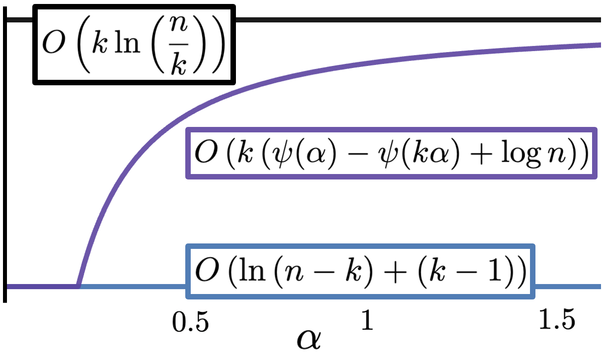
Figure 1: Visualizing the affect of the $\alpha$ parameter on this expectation term, with fixed $k$ and $n$. $\alpha$ essentially controls the “sparsity” of the distribution; a small $\alpha$ implies expected error closer to the theoretical lower bound.

This sum is maximized when all sizes are equal, so $|G_{i}|=n/k$. However, when the sum is smaller, we obtain a tighter bound than Proposition 9. In the most extreme case, when all group sizes equal one, except for a single (majority) group, the bound can be as good as $(k-1)+\log(n-k)$, which nearly matches the $\log n$ dependence of $\hat{p}$. And, in fact, we rarely observe uniform group sizes in practice, particularly when considering intersectional groups. Often, a small number of majority groups dominate. To better explain the error, take a standard Bayesian assumption that our group size vector is drawn from a Dirichlet distribution, $\mathcal{D}(\alpha,k)$. (Our Appendix contains notes and details on Dirichlet parameters and behavior for completeness.) In this case, we prove the following bound (see Appendix):

Theorem 10 (Error Upper Bound with Dirichlet Assumption).

Consider the Dirichlet distribution $\mathcal{D}(\alpha,k)$ with parameters $k,\alpha$ and let $\mathbf{g}\sim\mathcal{D}(\alpha,k)$ be a vector drawn from this distribution. If for each group $i$, $|G_{i}|=g_{i}/n$, then, letting $\psi$ denote the digamma function, we have:

$$\mathbb{E}\left[\sum_{i=1}^{k}\log|G_{i}|\right]\leq k\left(\psi(\alpha)-\psi(k\alpha)+\log n\right)$$ (6)

To better understand the bound of Theorem 10, please refer to Figure 1, which plots the bound in comparison to the weaker upper bound of $k\log(n/k)$ from Propostion 9, and in comparison to our informal lower bound $O(k+\log(n))$. As we can see, as the parameter $\alpha$ of the Dirichlet-distributed group size vectors varies from $[0.2,1.0)$, we interpolate between the lower and upper bound. Small $\alpha<1.0$ implies “sparsity”, i.e. one or two dominant entries in the vector $\mathbf{g}$. Overall, we frame this result as follows: In cases when minority groups in the data are relatively small compared to the majority groups, additional noise from privacy is expected to be small when aggregated.

Practical Implications of Theory

Our theory for stratified private mean estimation (PME) bounds worst case costs (Proposition 9) and expected costs (Theorem 10) for stratification. Much can be learned from these bounds practically. For a salient example, consider a sample of American Community Survey data for New York from 2018, where $n=196967$ and the RACE variable has $k=9$. The group size vector here is $v_{g}=[0.70,0.12,0.086,0.056,0.029,...]$. Using an iterative Monte Carlo approach to find a likely Dirichlet prior over $v_{g}$, we find $\alpha\approx 0.13$. Applying Proposition 9 and Theorem 10 then tells us that, for any setting of $R$ or $\epsilon$, our expected absolute error from stratification in estimating the mean for a given variable is approximately $\sim 80\%$ better than the worst case error, relative to the best case stratification error. This at least partially explains the strong performance of stratification empirically, seen in Figure 2. Put another way, our theory shows that, when the group sizes follow a Dirichlet distribution, then, as $\alpha\rightarrow 0$, the error of stratified PME scales with $O(k+\log(n)+R)$. This is close to the error of non-stratified PME, which scales as $O(\log(n)+R)$.

Adaptive Private Mean Estimation

In the previous section, we focused on bounding the additional error introduced by differential privacy, i.e., on $|\hat{p}-p|$, where $\hat{p}$ is a DP mean estimate and $p$ is the empirical mean. However, as we highlighted, this error is always in addition to the inherent statistic error $|\mu-p|$ between the true population mean $\mu$ and our empirical estimate $p$. It is well known that stratification can help reduce this statistic error (Cochran 1977; Botev and Ridder 2017). This helps explain the value of stratification in practice: extra error introduced by DP noise can be offset by reduced statistical error.

In particular, consider the case when each group has fixed variance $1$, but the means $\mu_{i}$ for the groups can differ substantially i.e. the overall data variance $\sigma$ is much larger than $1$. Then we expect statistical error on the order of $O(\sigma/\sqrt{n})$. On the other hand, if we assume we know exact group sizes and stratify, statistical error should scale as $O(1/\sqrt{n})$, which can be substantially better (Botev and Ridder 2017).

The naive mean estimation method analyzed in the previous section will likely not benefit from this scenario, since we will need to choose a large range $R$ (thus scaling our noise) if our group means differ substantially. However, adaptive mean estimation methods like Coinpress (Biswas et al. 2020) have been introduced that only depend logarithmically on $R$. In our experiments, we observe that the aggregate population level means of these methods can actually benefit from stratification.

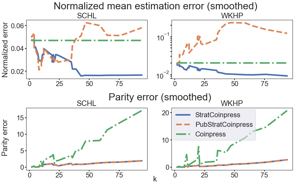
Figure 2: Comparisons of Coinpress and StratCoinpress on U.S. Census data from Folktables; SCHL is years spent in school (ordinal, 0-24), WKHP is hours worked per week (ordinal, 0-168). Top row shows normalized mean estimation error, bottom row shows parity error, both as the number of groups $k$ increases.

Measuring disparate impact of DP

We consider the following formalism for our setting to measure the impact of private mechanisms on subgroups in data. Intuitively, we want the error for any protected group in a population to be comparable to the error for other groups. Consider dataset $X$, which consists of $k$ strata $G_{1}\cup...\cup G_{k}$. Consider a non-private function that maps $X$ to a real-valued vector with values for each of the $k$ strata as well as a single global value $f(X):X\rightarrow\mathbb{R}^{k+1}$. A privatized version of $f(x)$ is denoted $\mathcal{M}_{f}(X):X\rightarrow\mathbb{R}^{k+1}$. Results for both on stratum $i$ are denoted $f(G_{i})$ and $\mathcal{M}_{f}(G_{i})$ respectively. Population level results are then $f(X)_{k+1}$ and $\mathcal{M}_{f}(X)_{k+1}$.

Definition 11 (Parity error).

Parity error $\phi$ is the average normalized absolute error in approximating $f(G_{i})$ for each stratum $i$, plus the normalized absolute error in approximating $f(X)_{k+1}$, weighted by a positive parameter $\omega$ that determines the emphasis on population-level accuracy:

$$\omega\left|\frac{f(X)_{k+1}-\mathcal{M}_{f}(X)_{k+1}}{f(X)_{k+1}}\right|+\sum_{i=1}^{k}\left|\frac{f(G_{i})-\mathcal{M}_{f}(G_{i})}{f(G_{i})}\right|$$ (7)

In Definition 11, $\omega$ weights the faithfulness to the overall population estimate in the sum. We emphasize faithfulness for the protected class strata, and so we set $\omega=\frac{1}{k}$ (weighting population-level estimates the same as any single-stratum estimate).

Data and Setup

We provide results of two experiments to validate the stratified adaptive private mean estimation approach. The first experiment (Figures 3, 7, 6) uses a synthetic mixture of $k$ Gaussians, over a dataset of size $n$, with Dirichlet parameter $\alpha$, to compare Coinpress and StratCoinpress. (The Appendix includes parameters for our synthetic Gaussians, which are chosen illustratively and are independent of our theory). Our second experiment (Figure 2) is on demographic census data for New York State from Folktables, a standard dataset in fair-ML literature (Ding et al. 2021). For consistency and comparability with prior work, we maintain Census variable codes in all of our plots and results; for example, SCHL is a discrete variable denoting years of education, and ranges from 0-24. For a complete list of Census variables, counts, marginals, and their corresponding meanings and domains, see the Appendix. We also use common, legally protected classes, like SEX, AGE and RAC1P, to create groups for stratification. Note that we present two stratified variants: StratCoinpress assumes direct access to the demographic weights necessary for stratification, while PubStratCoinpress calculates those weights on a smaller, non-overlapping public holdout set.

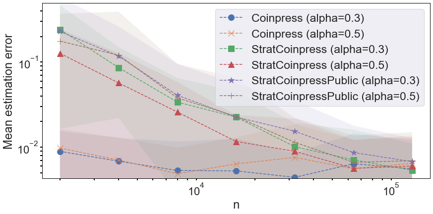
Figure 3: Mean estimation error, varying data size $n$ in synth Gaussian mixture (50 runs). Stratified variants converge to performance of non-stratified Coinpress as $n$ grows (for $n\geq 10000$, error $\leq 1\%$). In other words, with large samples, we don’t have to “pay” in global estimation error for a reduction in group-specific error.

In Figure 3, we depict the convergence of StratCoinpress to the performance of Coinpress as $n$ grows linearly. We do not report on disparate impact experiments with the synthetic data, as we can arbitrarily increase harm (measured by parity error) by increasing variance of the mixed Gaussian means. Figures 6 and 7 on this experiment, which show the effects of varying $k$ and $\alpha$, are available in the Appendix.

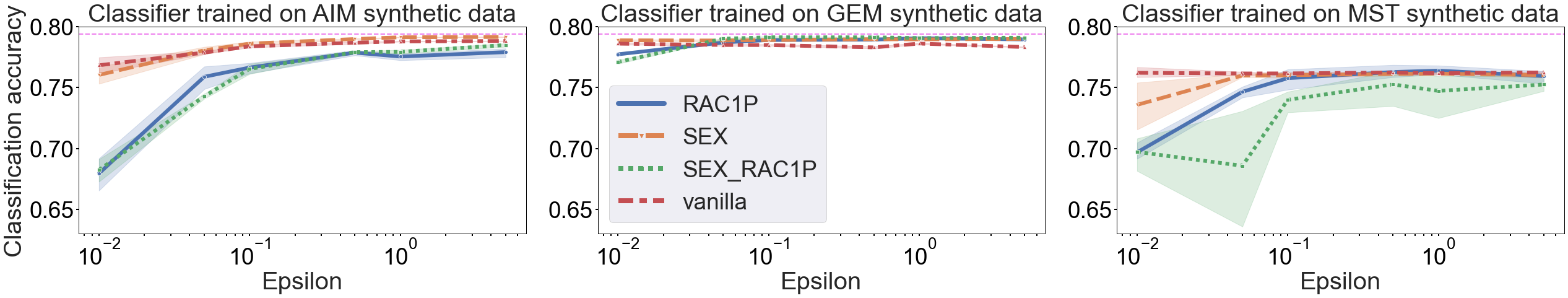
Figure 4: Performance of different stratified synthesizers, Folktables employment prediction. Note that variants of GEM and AIM approach a classifier trained on real data (accuracy $\approx 0.8$) as privacy budget increases. From the perspective of maintaining predictive utility, stratification appears to incur only minor costs, if any (for $\epsilon\geq 1$, difference $\leq 2\%$).

Effectiveness

In Figure 2, we show the effectiveness of a stratified adaptive mean estimation in practice. We vary $k$ by creating a different number of intersectional groups by combining $sex\in[0,1]$, $race\in[0,8]$, $age\in[0,4]$ (bucketed), and $physical$ $disability\in[0,1]$. The top row of Figure 2 shows that the error of the stratified variants of Coinpress is controlled in settings where the range of possible values is small relative to the total population size. In fact, when the subgroups are particularly meaningful (such as with SCHL, WKHP and JWMNP), stratification can sometimes improve on the overall mean estimates. Challenging settings for stratification are large continuous spaces such as with PINCP, where the strata-specific estimates (and, thus, the accuracy of aggregation) suffer from well-known private mean estimation challenges for wide range long-tailed distributions.

The bottom row of Figure 2 tells the story of harm reduction on subgroups in the data. Because private estimates are done over disjoint strata under composition (Def. 7), parity error can be tightly controlled by StratCoinpress. On the other hand, non-stratified Coinpress incurs substantial utility loss for most intersectional groups, because their mean differs significantly from the population-level mean.

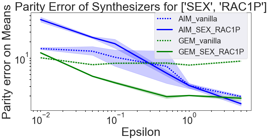
Figure 5: Parity error, where $f$ aggregates the error of means calculated on all variables in the Folktables employment prediction dataset. Here we contrast the two higher performing synthesizers: AIM (adaptive, lower predictive performance) and GEM (non-adaptive, higher predictive performance). Vanilla GEM struggles without explicit stratification, but by stratifying we can reduce parity error significantly (a reduction of $\geq 200\%$). Vanilla AIM’s budget and workload adaptivity has parity error benefits at low privacy budgets, though explicit stratification improves at higher budgets.

Stratified Data Synthesis

The disparate impacts of DP have been most commonly framed as occurring through private synthetic data (Bagdasaryan, Poursaeed, and Shmatikov 2019; Ganev, Oprisanu, and De Cristofaro 2022). Luckily, the principles of stratification (subset, estimate and aggregate) are not limited to mean estimation. Stratifying private synthesizers follows the same straightforward process: We learn separate parametric private distributions for each group-specific stratum. Then, to compose population-level data, we sample elements from strata-specific models proportionally to their representation in the full population. We do not offer theoretical bounds for private synthesizers as we did for mean estimation, as their guarantees are limited to specific query workloads selected during model fitting. This makes theoretical analysis challenging, and we leave it to future work.

Synthesizers and Privacy Settings

We conducted an extensive empirical evaluation on the viability of stratified synthetic data. We selected three state-of-the-art DP synthesizers: MST (McKenna, Miklau, and Sheldon 2021), GEM (Liu, Vietri, and Wu 2021), and AIM (McKenna et al. 2022). MST is data-aware, GEM is both data- and workload-aware, and AIM is data-, workload-, and privacy budget-aware (McKenna et al. 2022). Benchmarking DP synthesizers is non-trivial and computationally expensive (Rosenblatt et al. 2022). We ran our experiments on an NVIDIA T4 GPU cluster and on a high-performance CPU cluster. We ran our models on the same privacy settings as (McKenna et al. 2022), $\epsilon\in\{0.01,0.05,0.1,0.5,1.0,5.0\}$, representing a low to medium privacy budget regime. We trained 5 differently seeded models for each synthesizer at each privacy setting. Our models took over 200 hours of compute time to fit. We employ two naming conventions in labeling our figures: the first is that $\_$vanilla denotes the non-stratified version of the algorithm, and the second is that $\_$VARIABLE means that the algorithm stratifies explicitly along a set of dimensions (for example, SEX$\_$RAC1P implies separate models maintained for all subgroups induced by sex and race.)

Classification Setting

First, we found that stratification only seemed to harm the overall utility of private synthetic data in low privacy regimes ($\epsilon<0.1$). We demonstrate this on the Folktables employment prediction task (Ding et al. 2021) by training a classifier on DP synthetic versions of the data. Figure 4 shows that the strength of these classifiers increased as $\epsilon$ increased, implying that relationships in the data are maintained for nearly all variants, although we acknowledge the limitations of using classification as a proxy task higher-dimensional fidelity.

Parity Error Reduction

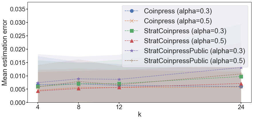
Figure 7: Comparing mean estimation error of Coinpress and StratCoinpress, over 50 runs. Mean estimation error, varying the number of groups $k$ in our synthetic Gaussian mixture. Note that error is low and relatively stable across reasonable values of $k$ groups in U.S. Census data.

Second, we find that stratified variants of all synthesizers reduce parity error (Definition 11). Figure 5 shows how additional privacy budget can generally improve the performance of the stratified variants (where the parity error function $f$ is the aggregate normalized difference of means across all variables in the Folktables employment task data). The best-performing synthesizer in our tests (GEM) also stratifies most gracefully, and provides the best parity error in nearly all $\epsilon$ parameter settings. We defer some experimental results to the Appendix, which further demonstrate that, for all synthesizers, as privacy budget increases: (1) the maximum disparity of all means gradually decreases (Figure 7a); (2) the demographic parity (Hardt, Price, and Srebro 2016) on the Folktables employment task increases towards 1 (Figure 7b); and (3) the maxmimum false negative rate difference between groups decreases (Figure 7c).

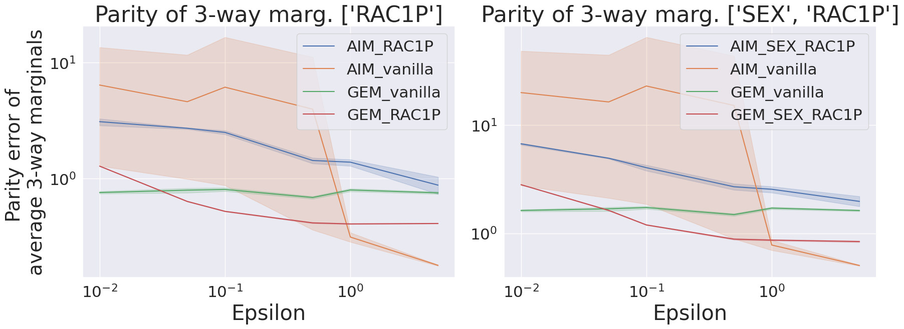
Figure 9: Parity error, where $f$ is the 3-way marginal function (McKenna et al. 2022). On left, error when strata are just the different $race$ groups. On right, error for intersectional $sex$ and $race$ groups.

Finally, in Figure 9 (also deferred to the Appendix), we use the All 3-Way Marginal workload error from (McKenna et al. 2022) as our function for parity error. This is a standard method of measuring performance of DP synthesizers: a $k$-way marginal for attribute set $S$ (where $|S|=k$) is a histogram over $x_{S}\in X$; marginal workload error is the average difference between these marginals run on real data and on private synthetic data (see Appendix or (McKenna et al. 2022) for more details). Figure 9 demonstrates that, in the case of non-budget adaptive algorithms like GEM, one can stratify and achieve low parity error and great overall performance. In the case of the budget-adaptive algorithm AIM, we see that it eventually has ample budget to adapt to all groups, and that the stratification might hurt performance. However, we rarely know what an acceptable budget setting is a priori; insufficient privacy budget for AIM (here, $\epsilon<1.0$) greatly increases the parity error of the vanilla adaptive algorithm relative to its stratified variant. Performance of the the stratified variant improves stably for all subgroups, and is thus much safer to use in regimes with a limited privacy budget, or when it is unclear how to set the budget.

Overall, we found that the stratified GEM variants convincingly outperformed MST and AIM with small privacy budget ($\epsilon\leq 1.0$). AIM did outperform GEM in the highest privacy regime of $\epsilon=5.0$, likely due to AIM’s ability to adapt and utilize “excess” privacy budget.

Limitations and future work

Our experimental results suggest that stratified synthetic data is safe given sufficient privacy budget, and that it often helps improve utility of subgroup data while preserving population-level utility, even in the case of adaptive algorithms. However, this fundamentally relies on good aggregation proportions, which may not always be available (say, in a medical context for a specific hospital). Though we believe that stratification provides a strong baseline for future work on adaptive DP algorithms with disparate impact protections, a stronger theoretical underpinning for stratified private synthesizers would allow for greater confidence in deployment. Additionally, our approach essentially targets parity error, and perhaps unsurprisingly trades off good performance there with worse performance by other metrics. Future work could formally characterize this trade-off by identifying the Pareto frontier of this dual optimization problem.

Conclusion

Reducing disparate impact in DP data release is a laudable goal that has received much attention in recent years. We showed that, when access to public estimates of group proportions in the data can be assumed, a stratified approach to disparate impact reduction is surprisingly effective, and that it does not significantly reduce — and sometimes even improves — the accuracy of population-level private statistics when the stratified private data is aggregated. With this work, we hope to encourage interest in principled methodologies for harm reduction when privatizing social data. We also hope that that practitioners will find the simple strategy we outlined here immediately applicable for private data release on sensitive data with protected classes.

Appendix A Complete proofs

Below we provide complete proofs and results to support the main body of the paper.

Proof of Proposition 9

The standard bound for a private mean estimator with the Laplace mechanism is given in the main paper body. We restate it here for convenience. With probability $1-O(\gamma)$, where $p$ is the empirical mean and $\hat{p}$ is the private empirical mean, then:

$$|\hat{p}-{p}|\leq O\left(\log(1/\gamma)\cdot\left(\frac{R+\sqrt{\log n/\gamma}}{n\epsilon}\right)\right)$$ (8)

Recall that our stratified synthesizer is defined as:

$$\hat{p}_{strat}=\frac{1}{n}\sum_{i=1}^{k}|G_{i}|\cdot\hat{p}_{i}$$ (9)

Where each $\hat{p}_{i}$ is a standard private empirical mean obtained through the Laplace mechanism and clipping (see Section Stratified Private Mean Estimation for details), with the bound given in Equation 8.

In Proposition 9, we bound the error between the stratified private empirical mean estimator $\hat{p}_{strat}$ and the non-private empirical mean $p$. We restate Proposition 9 below for convenience.

Proposition 9

[Worst Case Error Bound for Stratified Mean Estimation] Let $\hat{p}_{strat}$ be the estimator defined in Eq. (9). With probability $1-O(\gamma k)$,

$$|{p}-\hat{p}_{strat}|\leq O\left(\log(1/\gamma)\cdot\sqrt{k}\cdot\left(\frac{R+\sqrt{\log(n/k\gamma)}}{n\epsilon}\right)\right)$$ (10)

Proof.

Consider a single group $|G_{i}|$. When computing the standard DP estimator $\hat{p}_{i}$ we perform a clip operation for any $x\in G_{i}$ only if $|x|\geq R+\sqrt{\log|G_{i}|/\gamma}$. Recall that $x$ is assumed to be Gaussian distributed with mean $\mu_{i}$ and variance $1$. As is standard in the analysis of the unstratified estimator, we claim that, with high probability, no values of $x$ get clipped. In particular, we apply the standard concentration bound for univariate Gaussians:

$$\Pr[|x-\mathbb{E}[x]|\geq t]\leq e^{-t^{2}/2}.$$

Since $\mu_{i}$ is assumed to lie in $[-R,R]$, this bound implies that $|x|\geq R+\sqrt{\log|G_{i}|/\gamma}$ with probability less than $O(\gamma/|G_{i}|)$. So, by a union bound, no $x\in G_{i}$ gets clipped with probability at least $1-O(\gamma)$. Further union bounding across all $k$ groups, conclude that with probability at least $1-O(k\gamma)$, no $x$ gets clipped across the entire dataset. This fact makes it easy to write down an expression for ${p}-\hat{p}_{strat}$. In particular, we have:

$${p}-\hat{p}_{strat}=\frac{1}{n}(L_{1}+L_{2}+\ldots+L_{k}),$$

where $L_{i}$ is a centered Laplace random variable with parameter $b_{i}=\frac{2R+2\sqrt{\log|G_{i}|/\gamma}}{\epsilon}$. Following the standard definition of sub-exponential random variables found e.g in (Wainwright 2019), we can check that $L_{i}$ is sub-exponential with parameters $\nu_{i}=\alpha_{i}=2b_{i}$. Accordingly, by a standard argument, $\sum_{i=1}^{k}L_{i}$ is sub-exponential with parameters $\nu=2\sqrt{\sum_{i=1}^{k}b_{i}^{2}}$ and $\alpha=\max_{i}2b_{i}\leq 2\sqrt{\sum_{i=1}^{k}b_{i}^{2}}$ (Duchi 2021). We conclude via a standard sub-exponential tail bound (see e.g. Proposition 2.9 in (Wainwright 2019)) that for a fixed constant $c$,

$$\Pr\left[|{p}-\hat{p}_{strat}|\geq c\log(1/\gamma)\cdot\sqrt{\sum_{i=1}^{k}b_{i}^{2}}\right]\leq\gamma.$$ (11)

So, we are just left to bound $\sqrt{\sum_{i=1}^{k}b_{i}^{2}}$. To do so, note that:

$$\sum_{i=1}^{k}b_{i}^{2} =\frac{4}{\epsilon^{2}}\sum_{i=1}^{k}(R+\sqrt{\log|G_{i}|/\gamma})^{2}$$

$$\leq\frac{8}{\epsilon^{2}}\sum_{i=1}^{k}R^{2}+\log|G_{i}|/\gamma$$

$$=\frac{8}{\epsilon^{2}}\left(kR^{2}+k\log(1/\gamma)+\sum_{i=1}^{k}\log|G_{i}|\right)$$ (12)

In Lemma 12, we show that the $\max_{|G_{1}|,\ldots,|G_{k}|}\sum_{i=1}^{k}\log|G_{i}|\leq k\log(n/k)$ through an arithmetic mean argument, allowing us to upper bound Equation (A) by:

$$O\left(\frac{k}{\epsilon}^{2}\cdot\left(R^{2}+\log(n/k\gamma)\right)\right)$$ (13)

Plugging into (11) and using that for any positive $C,D$, $\sqrt{C^{2}+D^{2}}\leq C+D$ yields the proposition. ∎

Note: for clarity in Lemma 12, we use $|G_{i}|=g_{i}$.

Lemma 12.

For any $g_{1},...,g_{k}\in\mathbb{R}$, $g_{i}>0$ such that $\sum_{i=1}^{k}g_{i}=n$, we have $\sum_{i=1}^{k}{\log g_{i}}\leq k{\log(n/k)}$.

Proof.

Note that:

$$\sum_{i=1}^{k}\log g_{i}=\log g_{1}+...+\log g_{k}=\log\left(\prod_{i=1}^{k}g_{i}\right)$$ (14)

Consider any pair $g_{i}$ and $g_{j}$, where $g_{i}\neq g_{j}$, in $\prod_{i=1}^{k}g_{i}$. Let their arithmetic average be $\hat{g}_{ij}$ such that $g_{i}=\hat{g}_{ij}+d$ and $g_{j}=\hat{g}_{ij}-d$, where $d\neq 0$. Then

$$g_{i}+g_{j}=\hat{g}_{ij}+\hat{g}_{ij}$$ (15)

$$g_{i}\cdot g_{j}=\hat{g}_{ij}^{2}-d^{2}<\hat{g}_{ij}\cdot\hat{g}_{ij}$$ (16)

Thus, we can maintain the overall sum $\sum_{i=1}^{k}g_{i}=n$ while increasing the product $\prod_{i=1}^{k}g_{i}$ by setting $g_{i},g_{j}=\hat{g}_{ij}$ = $n/k$. Accordingly, the product can only be maximized when $g_{i}=g_{j}$ for all $i,j$ – in other words, when $g_{1},\ldots,g_{k}=n/k$. It follows that:

$$\log\left(\prod_{i=1}^{k}g_{i}\right) \leq\log\left(\prod_{i=1}^{k}n/k\right)$$

$$\sum_{i=1}^{k}\log g_{i} \leq\sum_{i=1}^{k}\log n/k.\qed$$

Proof of Theorem 10

We restate Theorem 10 here for convenience.

Consider the Dirichlet distribution $\mathcal{D}(\alpha,k)$ with parameters $k,\alpha$ and let $\mathbf{g}\sim\mathcal{D}(\alpha,k)$ be a vector drawn from this distribution. If for each group $i$, $|G_{i}|=g_{i}\cdot n$, then, letting $\psi$ denote the digamma function, we have:

$$\mathbb{E}\left[\sum_{i=1}^{k}\log|G_{i}|\right]\leq k\left(\psi(\alpha)-\psi(k\alpha)+\log n\right)$$ (17)

Proof.

We begin by applying linearity of expectation.

$$\mathbb{E}\left[\sum^{k}_{i=1}\log|G_{i}|\right] =k\mathbb{E}[\log g_{i}+\log n]\noindent$$ (18)

$$=k\log n+k\mathbb{E}[\log g_{i}]$$ (19)

Thus, the main challenge is deriving an expression for $\mathbb{E}[\log g_{i}]$ where $\mathbf{g}\sim\mathcal{D}(\alpha,k)$. We begin by applying law of the unconscious statistician.

$$\mathbb{E}[\log g_{i}]=\int_{0}^{1}\log g_{i}\mathcal{D}(g_{i}|\alpha)dg_{i}$$ (20)

We can marginalize $\mathcal{D}(g|\alpha)$ out into Beta distribution $\mathcal{B}(\alpha_{i},-\alpha_{i}+\sum^{k}\alpha_{i})$. As we assume symmetric $\alpha$, this becomes $\mathcal{B}(\alpha,k\alpha-\alpha)$. With substitution now, we have:

$$\mathbb{E}[\log g_{i}] =\int_{0}^{1}\log g_{i}\mathcal{B}(\alpha,k\alpha-\alpha)dg_{i}$$ (21)

$$=\int_{0}^{1}\log g_{i}\frac{1}{\beta(\alpha,k\alpha-\alpha)}g_{i}^{\alpha-1}(1-g_{i})^{k\alpha-\alpha-1}dg_{i}$$ (22)

Thus, we will take the square root of our final term. Note further that $\beta(z_{1},z_{2})=\frac{\Gamma(z_{1})\Gamma(z_{2})}{\Gamma(z_{1}+z_{2})}=\int_{0}^{1}t^{z_{1}-1}(1-t)^{z_{2}-1}dt$ is the $Beta$ function and $\Gamma(n)=(n-1)!$ is the $Gamma$ function. As both the $Beta$ function term and $\alpha$ are a constants, we can simplify further with:

$$=\frac{1}{\beta(\alpha,k\alpha-\alpha)}\frac{d}{d\alpha}\int_{0}^{1}g_{i}^{\alpha-1}(1-g_{i})^{k\alpha-\alpha-1}dg_{i}$$ (23)

Note that the integration term is now exactly a $Beta$ function, so we can simplify further.

$$=\frac{1}{\beta(\alpha,k\alpha-\alpha)}\frac{d\beta(\alpha,k\alpha-\alpha)}{d\alpha}$$ (24)

Which is now equivalent to taking the derivative of $\log(\beta(\alpha,k\alpha-\alpha))$ with respect to $\alpha$.

$$=\frac{d}{\alpha}\log(\beta(\alpha,k\alpha-\alpha))$$ (25)

Performing the $Gamma$ function expansion we get:

$$=\frac{d}{\alpha}\log\left(\frac{\Gamma(\alpha)\Gamma(k\alpha-\alpha)}{\Gamma(\alpha+k\alpha-\alpha)}\right)$$ (26)

$$=\frac{d}{\alpha}\log(\Gamma(\alpha))-\frac{d}{\alpha}\log(\Gamma(k\alpha))$$ (27)

The function $\psi(x)=\frac{d}{dx}\log(\Gamma(x))$ is commonly known as the digamma function.

We’ve now shown that:

$$\mathbb{E}[\log g_{i}]=\psi(\alpha)-\psi(k\alpha)$$ (28)

Plugging into (18) yields the result. ∎

Appendix B Additional details and experiments for Coinpress

In Algorithms 1 and 2, we restate Coinpress algorithms from (Biswas et al. 2020) for completeness. In Algorithm 3, we give a formalized version of the simple stratification algorithm discussed in the main paper body.

Algorithm 1 One Step Private Improvement of Mean Interval

Input: $n$ samples $X_{1\dots n}$ from $N(\mu,\sigma^{2})$, $[\ell,r]$ containing $\mu$, $\sigma^{2}$, $\rho_{s},\beta_{s}>0$
      Output: A $\rho_{s}$-zCDP interval $[\ell^{\prime},r^{\prime}]$

1:procedure UVM($X_{1\dots n},\ell,r,\sigma^{2},\rho_{s},\beta_{s}$)

2:     Project each $X_{i}$ into the interval $[\ell-\sigma\sqrt{2\log(2n/\beta_{s})},r+\sigma\sqrt{2\log(2n/\beta_{s})}]$.

3:     Let $\Delta=\frac{r-\ell+2\sigma\sqrt{2\log(2n/\beta_{s})}}{n}$.

4:     Compute $Z=\frac{1}{n}\sum_{i}X_{i}+Y$, where $Y\sim N\left(0,\left(\frac{\Delta}{\sqrt{2\rho_{s}}}\right)^{2}\right)$.

5:     return the interval $Z\pm\sqrt{2\left(\frac{\sigma^{2}}{n}+\left(\frac{\Delta}{\sqrt{2\rho_{s}}}\right)^{2}\right)\log(2/\beta_{s})}$.

6:end procedure

Algorithm 2 Private Confidence-interval-based Univariate Mean Estimation

Input: $n$ samples $X_{1\dots n}$ from $N(\mu,\sigma^{2})$, $[\ell,r]$ containing $\mu$, $\sigma^{2}$, $t\in\mathbb{N}^{+}$, $\rho_{1\dots t},\beta>0$
      Output: A $(\sum_{i=1}^{t}\rho_{i})$-zCDP estimate of $\mu$

1:procedure UVMRec($X_{1\dots n},\ell,r,\sigma^{2},t,\rho_{1\dots t},\beta$)

2:     Let $\ell_{0}=\ell,r_{0}=r$.

3:     for $i\in[t-1]$ do

4:         $[\ell_{i},r_{i}]=\textsc{UVM}(X_{1\dots n},\ell_{i-1},r_{i-1},\sigma^{2},\rho_{i},\beta/4(t-1))$.

5:     end for

6:     $[\ell_{t},r_{t}]=\textsc{UVM}(X_{1\dots n},\ell_{t-1},r_{t-1},\sigma^{2},\rho_{t},\beta/4)$.

7:     return the midpoint of $[\ell_{i},r_{i}]$.

8:end procedure

Algorithm 3 Stratified Univariate Coinpress

Input: Strata $X^{1}\cup...\cup X^{k}=X$ where each stratum $X^{i}\sim N(\mu_{i},\sigma_{i}^{2})$ and $X\sim N(\mu,\sigma^{2})$ overall, $|X|=n$, $[\ell,r]$ containing all $\mu_{i},\sigma_{i}$ and $\mu$, $\sigma^{2}$, $t\in\mathbb{N}^{+}$, $\rho_{1\dots t},\beta=\sum_{i=1}^{k}\beta_{i}>0$, weights $\omega_{1},...\omega_{k}$
      Output: A $(\sum_{i=1}^{t}\rho_{i})$-zCDP estimate of global $\hat{\mu}$ as well as $(\sum_{i=1}^{t}\rho_{i})$-zCDP estimates of $\hat{\mu_{1}},...,\hat{\mu_{k}}$ for each stratum.

1:procedure StratCoinpress($X^{1}\cup...\cup X^{k}=X,\ell,r,\sigma^{2},t,\rho_{1\dots t},\beta_{1},...,\beta_{k}$, $\omega_{1},...\omega_{k}$)

2:     for $i\in k$ do

3:         $\mu_{i}=\textsc{UVMRec}(X_{1\dots n}^{i},\ell,r,\sigma^{2},\rho_{i},\beta_{i})$.

4:     end for

5:     $\hat{\mu}=\frac{1}{k}\sum^{k}_{i=1}\omega_{i}\mu_{i}$.

6:     return $\hat{\mu},\{\hat{\mu_{1}},...,\hat{\mu_{k}}\}$.

7:end procedure

Additional plots for coinpress experiments

We provide an exhaustive plot for convergence of stratified Coinpress variants in Figure 6.

Here we also state the generative model for the Gaussian data. We draw a Dirichlet vector $\mathbf{v}\sim\mathcal{D}(k,\alpha)$. Then, we fix uniformly random parameters for each $k$ Gaussian (in our tests, $\sigma_{i}\sim\mathcal{U}(\ell=0.1,u=2.0)$ and $\mu_{i}\sim\mathcal{N}(0,1.0)$. Finally, using the weights of $\mathbf{v}$, we draw $k$ Gaussian samples $G_{i}\sim N(\mu_{i},\sigma_{i})$, where $|G_{i}|=\frac{n}{k}$. This is the data model used to produce our synthetic mean estimation results.

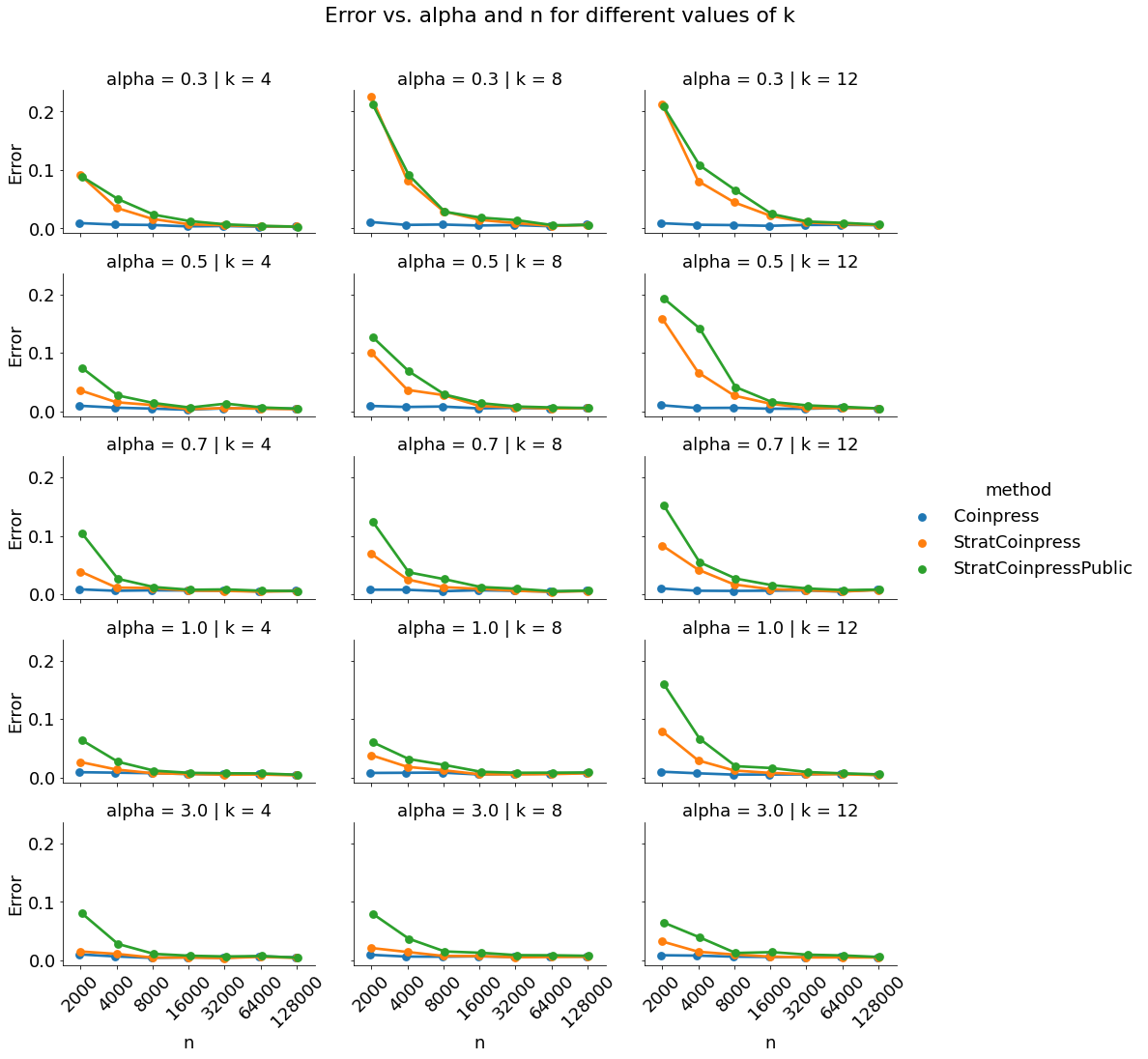
Figure 6: Complete results for synthetic Coinpress comparisons.

Note on $(\rho)$-zCDP composition

Coinpress relies on composition rules for zero-concentrated differential privacy.

Sequential composition: If $\mathcal{M}$ and $\mathcal{M^{\prime}}$ satisfy $(\rho_{1})$-zCDP and $(\rho_{2})$-zCDP respectively, then the sequential $\mathcal{M}^{*}(X)=(\mathcal{M}(X),\mathcal{M^{\prime}}(X))$ satisfies $(\rho_{1}+\rho_{2})$-zCDP.

Parallel composition: if $\mathcal{M}$ satisfies $\rho$-zCDP, and $\{X_{1},...,X_{k}\}$ are disjoint, then the parallel mechanism $\mathcal{M}^{*}(X)=(\mathcal{M}(X_{1}),...,\mathcal{M}(X_{k}))$ also satisfies $\rho$-zCDP.

Appendix C Additional Plots and Notes on Private Data Synthesizers

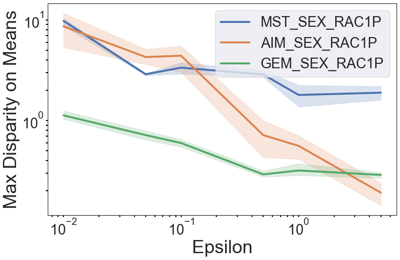
(a) Max disparity.

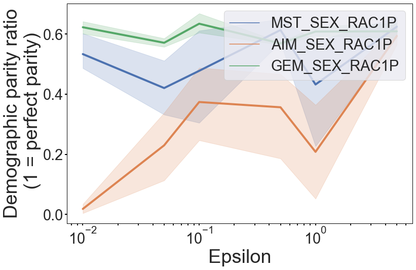
(b) Demographic parity.

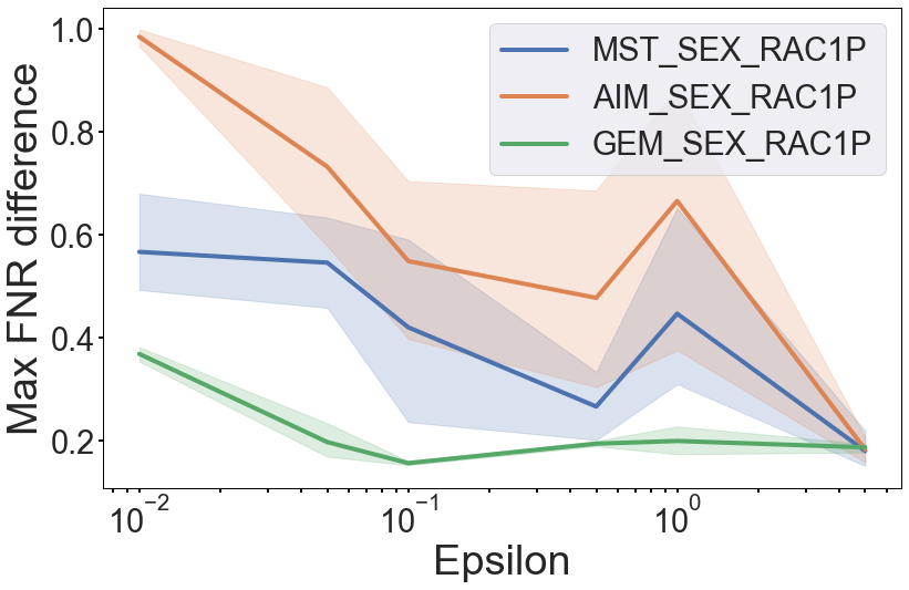
(c) Max FNR Difference.

Discussion of challenges in analyzing stratified synthetic data

Consider a fundamental private data synthesizer like Multiplicative Weights Exponential Mechanism (MWEM) (Hardt, Ligett, and McSherry 2012). MWEM introduced the underlying strategy of many state-of-the-art private synthesizers used today: (1) Select: privately select a relatively small set of the most informative measurements over your data (in MWEM, this is done with the exponential mechanism (Dwork, Roth et al. 2014)). (2) Measure: privately measure that set on your real data (MWEW uses the Laplace mechanism in this step). (3) Project: as a post-processing step, project theses private measurements onto a parameterized distribution over the domain of your data (MWEM maintains a histogram distribution and uses multiplicative weights for updates).

The challenge in analyzing stratified and non-stratified private data synthesizers lies in the initial Select step. Were we to fix the set of selected measurements across all strata, then the aggregation step composes gracefully. In fact, in a non-private setting, the distributional weights for each variable for the entire population would simply be a weighted combination of the distributional weights for each strata. However, we are not guaranteed that there will be overlap in measurements selected by each strata specific select step the select step run on the overall population. For example, consider the stylized example where we limit ourselves to a single measurement in the select step. The most informative measurement candidate for the full population could be the second most informative candidate for each stratum. In this case, we would have no direct measurements for the full population, and thus no population level utility guarantees.

Marginals

The following is adapted from (McKenna et al. 2022). They define marginals as a method to capture low-dimensional structure common in high-dimensional data distributions. Informally, a marginal for a set of attributes $S$ is essentially a histogram over $X_{S}$: it is a table that counts the number of occurrences of each $t\in\Omega_{S}$. Sometimes we can refer to the below functions as marginal queries, and thus a marginal is the resulting vector of counts $M_{S}(D)$.

Definition 13 (Marginal (McKenna, Miklau, and Sheldon 2021; McKenna et al. 2022)).

Let $S\subseteq[d]$ be a subset of attributes, $\Omega_{S}=\prod_{i\in S}\Omega_{S}$, $n_{S}=|\Omega_{S}|$, and $X_{S}=(X_{i})_{i\in S}$. The marginal on $S$ is a vector $\mu\in\mathbb{R}^{n_{S}}$, indexed by domain elements $t\in\Omega_{S}$, such that each entry is a count, i.e., $\mu[t]=\sum_{x\in D}\mathbf{1}[x_{S}=t]$. We let $M_{S}:\mathcal{D}\rightarrow\mathbb{R}^{n_{S}}$ denote the function that computes the marginal on $S$, i.e., $\mu=M_{S}(D)$.

Workload Error

Adapted from (McKenna et al. 2022), the following defines a standard method for evaluating private synthetic data used to generate Figure 9. We define a workload as a collection of marginal queries that synthetic data should preserve. The marginal based utility measure underlying 3-Way Marginal Error is stated in Definition 14, framed as general error for any workload of queries.

Definition 14 (Workload Error (McKenna, Miklau, and Sheldon 2021; McKenna et al. 2022)).

A workload $W$ consists of a list of marginal queries $S_{1},\dots,S_{k}$ where $S_{i}\subseteq[d]$, together with associated weights $c_{i}\geq 0$. The error of a synthetic dataset $\hat{D}$ is defined as:

$$\text{Error}(D,\hat{D})=\frac{1}{k\cdot|D|}\sum_{i=1}^{k}c_{i}\left(||M_{S_{i}}(D)-M_{S_{i}}(\hat{D})||_{1}\right)$$

Appendix D Additional Data Description

	SEX	DIS	NATIVITY	RAC1P	AGEP	SCHL	WKHP	JWMNP	PINCP
Count	196967	196967	196967	196967	196967	191372	103756	87355	166318
Mean	1.517	1.865	1.196	2.186	41.831	16.39	37.562	33.464	46657.585
Std	0.5	0.341	0.397	2.342	23.554	5.686	13.105	26.601	76027.3
Range	[1 , 2]	[1 , 2]	[1 , 2]	[1 , 9]	[0 , 95]	[1 , 24]	[1 , 99]	[1 , 138]	[-8300 , 1423000]
Median	2	2	1	1	42	18	40	30	26500

Table 1: This table gives descriptive information on columns from Folktables used in the mean estimation task.

	AGEP	SCHL	MAR	DIS	ESP	MIL	DREM	SEX	RAC1P	ESR
Mean	1.687	2.834	3.043	1.865	0.543	3.183	1.852	1.517	2.186	0.464
Std	1.234	1.246	1.867	0.341	1.587	1.547	0.471	0.5	2.342	0.499
Range	[0 , 4]	[0 , 4]	[1 , 5]	[1 , 2]	[0 , 8]	[0 , 4]	[0 , 2]	[1 , 2]	[1 , 9]	[0 , 1]
Median	2	3	3	2	0	4	2	2	1	0

Table 2: This table gives descriptive information on columns from Folktables used in the private data synthesis task. All columns are fully represented (count $=196967$).

SEX	RAC1P	Count
Female	White	70881
Male	White	67593
Female	Black	12947
Male	Black	11077
Female	Asian	8900
Male	Asian	8130
Female	Some other race alone	5668
Male	Some other race alone	5296
Female	Two or more races	3026
Male	Two or more races	2620
Male	American Indian alone	277
Female	American Indian alone	231
Male	American Indian and/or Alaska Native (tribes no…	125
Female	American Indian and/or Alaska Native (tribes no…	119
Male	Native Hawaiian	42
Female	Native Hawaiian	30
Female	Alaska Native alone	3
Male	Alaska Native alone	2

Table 3: This table provides the exact group size breakdown for the ACSEmployment task from Folktables (New York data), used in the synthetic data experiments.

Below we also give descriptions of each Census variable used, and interpretations of their values. These are taken directly from (Ding et al. 2021), who in turn took them from public ACS documentation.

1. AGEP (Age): Range of values:

   • 0 - 99 (integers)

   • 0 indicates less than 1 year old.

2. SCHL (Educational attainment): Range of values:

   • N/A (less than 3 years old)

   • 1: No schooling completed

   • 2: Nursery school/preschool

   • 3: Kindergarten

   • 4: Grade 1

   • 5: Grade 2

   • 6: Grade 3

   • 7: Grade 4

   • 8: Grade 5

   • 9: Grade 6

   • 10: Grade 7

   • 11: Grade 8

   • 12: Grade 9

   • 13: Grade 10

   • 14: Grade 11

   • 15: 12th Grade - no diploma

   • 16: Regular high school diploma

   • 17: GED or alternative credential

   • 18: Some college but less than 1 year

   • 19: 1 or more years of college credit but no degree

   • 20: Associate’s degree

   • 21: Bachelor’s degree

   • 22: Master’s degree

   • 23: Professional degree beyond a bachelor’s degree

   • 24: Doctorate degree

3. MAR (Marital status): Range of values:

   • 1: Married

   • 2: Widowed

   • 3: Divorced

   • 4: Separated

   • 5: Never married or under 15 years old

4. WKHP (Usual hours worked per week past 12 months): Range of values:

   • N/A (less than 16 years old / did not work during the past 12 months)

   • 1 - 98 integer valued: usual hours worked

   • 99: 99 or more usual hours

5. SEX (Sex): Range of values:

   • 1: Male

   • 2: Female

6. RAC1P (Recoded detailed race code): Range of values:

   • 1: White alone

   • 2: Black or African American alone

   • 3: American Indian alone

   • 4: Alaska Native alone

   • 5: American Indian and Alaska Native tribes specified, or American Indian or Alaska Native, not specified and no other races

   • 6: Asian alone

   • 7: Native Hawaiian and Other Pacific Islander alone

   • 8: Some Other Race alone

   • 9: Two or More Races

7. DIS (Disability recode): Range of values:

   • 1: With a disability

   • 2: Without a disability

8. ESP (Employment status of parents): Range of values:

   • N/A (not own child of householder, and not child in subfamily)

   • 1: Living with two parents: both parents in labor force

   • 2: Living with two parents: Father only in labor force

   • 3: Living with two parents: Mother only in labor force

   • 4: Living with two parents: Neither parent in labor force

   • 5: Living with father: Father in the labor force

   • 6: Living with father: Father not in labor force

   • 7: Living with mother: Mother in the labor force

   • 8: Living with mother: Mother not in labor force

9. MIL (Military service): Range of values:

   • N/A (less than 17 years old)

   • 1: Now on active duty

   • 2: On active duty in the past, but not now

   • 3: Only on active duty for training in Reserves/National Guard

   • 4: Never served in the military

10. DREM (Cognitive difficulty): Range of values:

    • N/A (less than 5 years old)

    • 1: Yes

    • 2: No

11. PINCP (Total person’s income): Range of values:

    • integers between -19997 and 4209995 to indicate income in US dollars

    • loss of $19998 or more is coded as -19998.

    • income of $4209995 or more is coded as 4209995.

12. ESR (Employment status recode): an individual’s label is 1 if ESR == 1, and 0 otherwise.

13. JWMNP (Travel time to work): Range of values:

    • N/A (not a worker or a worker that worked at home)

    • integers 1 - 200 for minutes to get to work

    • top-coded at 200 so values above 200 are coded as 200

14. WKHP (Usual hours worked per week past 12 months): Range of values:

    • N/A (less than 16 years old / did not work during the past 12 months)

    • 1 - 98 integer valued: usual hours worked

    • 99: 99 or more usual hours

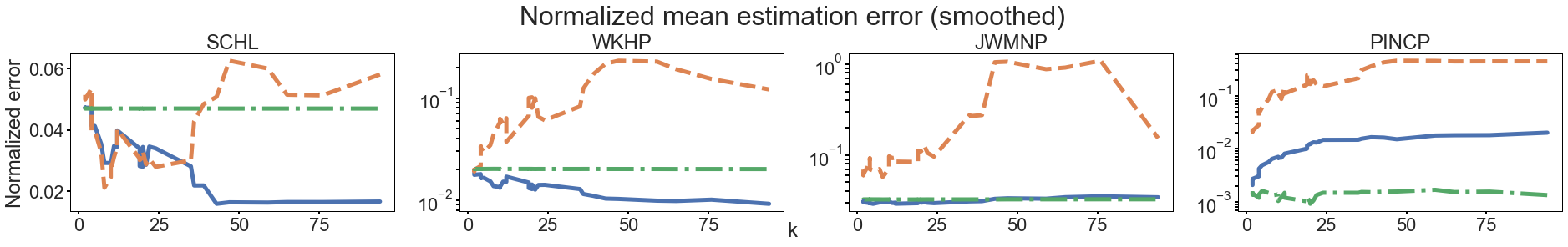
(a)

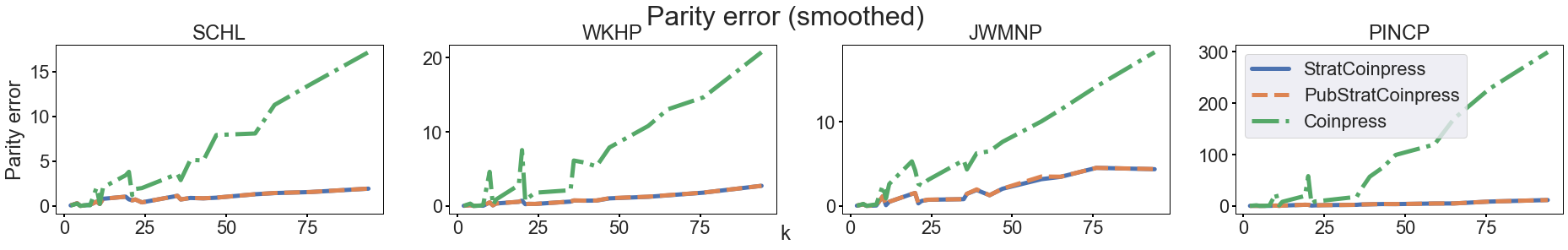
(b)

Figure 8: (Full version of 2) Comparisons of Coinpress and StratCoinpress on U.S. Census data from Folktables for the Mobility task (Ding et al. 2021); SCHL is years spent in school (ordinal, 0-24), WKHP is hours worked per week (ordinal, 0-168), JWMNP is average drive time (ordinal, 0-400) and PINCP is income (continuous). Top row shows normalized mean estimation error, bottom row shows parity error, both as the number of groups $k$ increases.

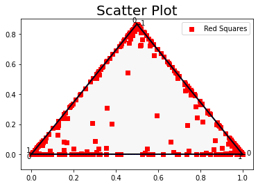
(a)

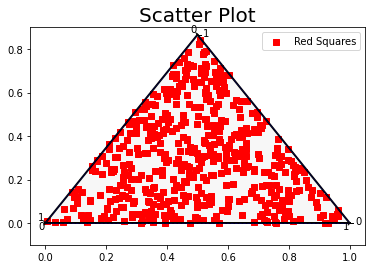
(b)

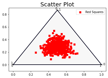
(c)

Figure 10: $k$=3 random vectors, $\mathcal{D}(\alpha=\{0.1,1,10\})$

Appendix E The Dirichlet distribution

A Dirichlet distribution ($\mathcal{D}$) has a probability density function given by the following, where $k\geq 2$, $\alpha_{i}>0$, and $B$ is a beta function expressed in terms of a gamma function

$$f(x_{1},...,x_{k};\alpha_{1},...,\alpha_{k})=\frac{1}{B(\{\alpha_{i}\})}\prod_{i=1}^{k}x_{i}^{\alpha_{i}-1}$$ (29)

$$B(\{\alpha_{i}\})=\frac{\prod_{i=1}^{k}\Gamma(\alpha_{i})}{\Gamma(\sum^{k}\alpha_{i})}$$ (30)

A special case, and the one we primarily consider here, is the symmetric Dirichlet distribution, when $\alpha_{1},...,\alpha_{k}=\alpha$.

$$f(x_{1},...,x_{k};\alpha)=\frac{\Gamma(\alpha k)}{\Gamma(\alpha)^{k}}\prod_{i=1}^{k}x_{i}^{\alpha-1}$$ (31)

Canonically, the Dirichlet distribution is known as the “distribution over distributions,” and is used to draw a random vector of size $k$, where the entries of that vector sum to 1. The distribution of those entries is governed, in the symmetric case, by a single parameter $\alpha$. When $\alpha<1$, the magnitude of the $k$ entries in the vector are distributed less evenly, and when $\alpha>1$ we see a more even distribution. We can visualize this nicely when $k=3$ by drawing a set of 100 random dirichlet vectors and plotting them in Figure 10.

References

- Abadi et al. (2016) Abadi, M.; Chu, A.; Goodfellow, I.; McMahan, H. B.; Mironov, I.; Talwar, K.; and Zhang, L. 2016. Deep learning with differential privacy. In Proc. of the 2016 ACM SIGSAC Conf. on CCS, 308–318.
- Ashtiani and Liaw (2022) Ashtiani, H.; and Liaw, C. 2022. Private and polynomial time algorithms for learning gaussians and beyond. In Conf on Learning Theory, 1075–1076. PMLR.
- Aydore et al. (2021) Aydore, S.; Brown, W.; Kearns, M.; Kenthapadi, K.; Melis, L.; Roth, A.; and Siva, A. A. 2021. Differentially private query release through adaptive projection. In International Conf on Machine Learning, 457–467. PMLR.
- Bagdasaryan, Poursaeed, and Shmatikov (2019) Bagdasaryan, E.; Poursaeed, O.; and Shmatikov, V. 2019. Differential privacy has disparate impact on model accuracy. Advances in neural information processing systems, 32.
- Barocas and Selbst (2016) Barocas, S.; and Selbst, A. D. 2016. Big data’s disparate impact. California law review, 671–732.
- Bie, Kamath, and Singhal (2022) Bie, A.; Kamath, G.; and Singhal, V. 2022. Private Estimation with Public Data. arXiv:2208.07984.
- Biswas et al. (2020) Biswas, S.; Dong, Y.; Kamath, G.; and Ullman, J. 2020. Coinpress: Practical private mean and covariance estimation. Advances in Neural Information Processing Systems, 33: 14475–14485.
- Boedihardjo, Strohmer, and Vershynin (2022) Boedihardjo, M.; Strohmer, T.; and Vershynin, R. 2022. Private sampling: a noiseless approach for generating differentially private synthetic data. SIAM Journal on Mathematics of Data Science, 4(3): 1082–1115.
- Botev and Ridder (2017) Botev, Z.; and Ridder, A. 2017. Variance Reduction, 1–6. John Wiley & Sons, Ltd. ISBN 9781118445112.
- Bun and Steinke (2016) Bun, M.; and Steinke, T. 2016. Concentrated differential privacy: Simplifications, extensions, and lower bounds. In Theory of Cryptography: 14th International Conf, TCC 2016-B, Beijing, China, October 31-November 3, 2016, Proceedings, Part I, 635–658. Springer.
- Bureau (2021) Bureau, U. 2021. Disclosure avoidance for the 2020 census: An introduction.
- Cai et al. (2021) Cai, K.; Lei, X.; Wei, J.; and Xiao, X. 2021. Data synthesis via differentially private markov random fields. Proc. of the VLDB Endowment, 14(11): 2190–2202.
- Cheng et al. (2021) Cheng, V.; Suriyakumar, V. M.; Dullerud, N.; Joshi, S.; and Ghassemi, M. 2021. Can you fake it until you make it? impacts of differentially private synthetic data on downstream classification fairness. In Proc. of the 2021 ACM Conf. on FAccT, 149–160.
- Christ, Radway, and Bellovin (2022) Christ, M.; Radway, S.; and Bellovin, S. M. 2022. Differential Privacy and Swapping: Examining De-Identification’s Impact on Minority Representation and Privacy Preservation in the US Census. In 2022 IEEE Symposium on Security and Privacy (SP), 1564–1564. IEEE Computer Society.
- Cochran (1977) Cochran, W. G. 1977. Sampling techniques. John Wiley & Sons.
- Corbett-Davies and Goel (2018) Corbett-Davies, S.; and Goel, S. 2018. The measure and mismeasure of fairness: A critical review of fair machine learning. arXiv:1808.00023.
- Cormode et al. (2018) Cormode, G.; Jha, S.; Kulkarni, T.; Li, N.; Srivastava, D.; and Wang, T. 2018. Privacy at scale: Local differential privacy in practice. In Proc. of the 2018 International Conf on Management of Data, 1655–1658.
- Cummings et al. (2019) Cummings, R.; Gupta, V.; Kimpara, D.; and Morgenstern, J. 2019. On the compatibility of privacy and fairness. In Adjunct Publication of the 27th Conf on User Modeling, Adaptation and Personalization, 309–315.
- Ding, Kulkarni, and Yekhanin (2017) Ding, B.; Kulkarni, J.; and Yekhanin, S. 2017. Collecting telemetry data privately. Advances in Neural Information Processing Systems, 30.
- Ding et al. (2021) Ding, F.; Hardt, M.; Miller, J.; and Schmidt, L. 2021. Retiring adult: New datasets for fair machine learning. Advances in neural information processing systems, 34: 6478–6490.
- Dinur and Nissim (2003) Dinur, I.; and Nissim, K. 2003. Revealing information while preserving privacy. In Proc. of the twenty-second ACM SIGMOD-SIGACT-SIGART symposium on Principles of database systems, 202–210.
- Duchi (2021) Duchi, J. 2021. Lecture Notes for Statistics 311/Electrical Engineering 377.
- Dwork and Lei (2009) Dwork, C.; and Lei, J. 2009. Differential privacy and robust statistics. In Proc. of the forty-first annual ACM symposium on Theory of computing, 371–380.
- Dwork, Roth et al. (2014) Dwork, C.; Roth, A.; et al. 2014. The algorithmic foundations of differential privacy. Foundations and Trends in Theoretical Computer Science, 9(3-4): 211–407.
- Dwork et al. (2017) Dwork, C.; Smith, A.; Steinke, T.; and Ullman, J. 2017. Exposed! a survey of attacks on private data. Annu. Rev. Stat. Appl, 4(1): 61–84.
- Dwork et al. (2015) Dwork, C.; Smith, A.; Steinke, T.; Ullman, J.; and Vadhan, S. 2015. Robust traceability from trace amounts. In 2015 IEEE 56th Annual Symposium on Foundations of Computer Science, 650–669. IEEE.
- Erlingsson, Pihur, and Korolova (2014) Erlingsson, Ú.; Pihur, V.; and Korolova, A. 2014. Rappor: Randomized aggregatable privacy-preserving ordinal response. In Proc. of the 2014 ACM SIGSAC, 1054–1067.
- Feldman et al. (2015) Feldman, M.; Friedler, S. A.; Moeller, J.; Scheidegger, C.; and Venkatasubramanian, S. 2015. Certifying and removing disparate impact. In Proc. of the 21th ACM SIGKDD, 259–268.
- Fioretto et al. (2022) Fioretto, F.; Tran, C.; Van Hentenryck, P.; and Zhu, K. 2022. Differential privacy and fairness in decisions and learning tasks: A survey. arXiv:2202.08187.
- Friedman and Nissenbaum (1996) Friedman, B.; and Nissenbaum, H. 1996. Bias in Computer Systems. ACM Trans. Inf. Syst., 14(3): 330–347.
- Ganev, Oprisanu, and De Cristofaro (2022) Ganev, G.; Oprisanu, B.; and De Cristofaro, E. 2022. Robin Hood and Matthew Effects: Differential Privacy Has Disparate Impact on Synthetic Data. In International Conf. on Machine Learning, 6944–6959. PMLR.
- Garrow (2014) Garrow, D. J. 2014. Toward a Definitive History of Griggs v. Duke Power Co. Vand. L. Rev., 67: 197.
- Groshen and Goroff (2022) Groshen, E. L.; and Goroff, D. 2022. Disclosure avoidance and the 2020 Census: What do researchers need to know. Harvard Data Science Review.
- Hardt, Ligett, and McSherry (2012) Hardt, M.; Ligett, K.; and McSherry, F. 2012. A simple and practical algorithm for differentially private data release. Advances in neural information processing systems, 25.
- Hardt, Price, and Srebro (2016) Hardt, M.; Price, E.; and Srebro, N. 2016. Equality of opportunity in supervised learning. Advances in neural information processing systems, 29.
- Hawes (2020) Hawes, M. B. 2020. Implementing differential privacy: Seven lessons from the 2020 United States Census. Harvard Data Science Review, 2(2).
- Ji and Elkan (2013) Ji, Z.; and Elkan, C. 2013. Differential privacy based on importance weighting. Machine learning, 93: 163–183.
- Ji, Lipton, and Elkan (2014) Ji, Z.; Lipton, Z. C.; and Elkan, C. 2014. Differential privacy and machine learning: a survey and review. arXiv:1412.7584.
- Kamath et al. (2022) Kamath, G.; Mouzakis, A.; Singhal, V.; Steinke, T.; and Ullman, J. 2022. A private and computationally-efficient estimator for unbounded gaussians. In Conf on Learning Theory, 544–572. PMLR.
- Kamath et al. (2019) Kamath, G.; Sheffet, O.; Singhal, V.; and Ullman, J. 2019. Differentially private algorithms for learning mixtures of separated gaussians. Advances in Neural Information Processing Systems, 32.
- Kamath, Singhal, and Ullman (2020) Kamath, G.; Singhal, V.; and Ullman, J. 2020. Private mean estimation of heavy-tailed distributions. In Conf on Learning Theory, 2204–2235. PMLR.
- Karwa and Vadhan (2017) Karwa, V.; and Vadhan, S. 2017. Finite sample differentially private Confidence intervals. arXiv preprint arXiv:1711.03908.
- Kenny et al. (2021) Kenny, C. T.; Kuriwaki, S.; McCartan, C.; Rosenman, E. T.; Simko, T.; and Imai, K. 2021. The use of differential privacy for census data and its impact on redistricting: The case of the 2020 US Census. Science advances, 7(41): eabk3283.
- Lin et al. (2023) Lin, S.; Bun, M.; Gaboardi, M.; Kolaczyk, E. D.; and Smith, A. 2023. Differentially Private Confidence Intervals for Proportions under Stratified Random Sampling. arXiv preprint arXiv:2301.08324.
- Liu et al. (2021a) Liu, T.; Vietri, G.; Steinke, T.; Ullman, J.; and Wu, S. 2021a. Leveraging public data for practical private query release. In International Conf. on Machine Learning, 6968–6977. PMLR.
- Liu, Vietri, and Wu (2021) Liu, T.; Vietri, G.; and Wu, S. Z. 2021. Iterative methods for private synthetic data: Unifying framework and new methods. Advances in Neural Information Processing Systems, 34: 690–702.
- Liu et al. (2021b) Liu, X.; Kong, W.; Kakade, S.; and Oh, S. 2021b. Robust and differentially private mean estimation. Advances in neural information processing systems, 34: 3887–3901.
- McKenna, Miklau, and Sheldon (2021) McKenna, R.; Miklau, G.; and Sheldon, D. 2021. Winning the NIST Contest: A scalable and general approach to differentially private synthetic data. arXiv:2108.04978.
- McKenna et al. (2022) McKenna, R.; Mullins, B.; Sheldon, D.; and Miklau, G. 2022. Aim: An adaptive and iterative mechanism for differentially private synthetic data. arXiv:2201.12677.
- McKenna, Sheldon, and Miklau (2019) McKenna, R.; Sheldon, D.; and Miklau, G. 2019. Graphical-model based estimation and inference for differential privacy. In International Conf on Machine Learning, 4435–4444. PMLR.
- Mironov (2017) Mironov, I. 2017. Rényi differential privacy. In 2017 IEEE 30th computer security foundations symposium (CSF), 263–275. IEEE.
- Mitchell et al. (2021) Mitchell, S.; Potash, E.; Barocas, S.; D’Amour, A.; and Lum, K. 2021. Algorithmic fairness: Choices, assumptions, and definitions. Annual Review of Statistics and Its Application, 8: 141–163.
- Pujol et al. (2020) Pujol, D.; McKenna, R.; Kuppam, S.; Hay, M.; Machanavajjhala, A.; and Miklau, G. 2020. Fair decision making using privacy-protected data. In Proceedings of FAccT 2020, 189–199.
- Rosenblatt et al. (2022) Rosenblatt, L.; Holovenko, A.; Rumezhak, T.; Stadnik, A.; Herman, B.; Stoyanovich, J.; and Howe, B. 2022. Epistemic Parity: Reproducibility as an Evaluation Metric for Differential Privacy. arXiv:2208.12700.
- Rosenblatt et al. (2020) Rosenblatt, L.; Liu, X.; Pouyanfar, S.; de Leon, E.; Desai, A.; and Allen, J. 2020. Differentially private synthetic data: Applied evaluations and enhancements. arXiv:2011.05537.
- Ruggles et al. (2019) Ruggles, S.; Fitch, C.; Magnuson, D.; and Schroeder, J. 2019. Differential privacy and census data: Implications for social and economic research. In AEA papers and proceedings, volume 109, 403–408. American Economic Association 2014 Broadway, Suite 305, Nashville, TN 37203.
- Tao et al. (2021) Tao, Y.; McKenna, R.; Hay, M.; Machanavajjhala, A.; and Miklau, G. 2021. Benchmarking differentially private synthetic data generation algorithms. arXiv:2112.09238.
- Tran, Dinh, and Fioretto (2021) Tran, C.; Dinh, M.; and Fioretto, F. 2021. Differentially private empirical risk minimization under the fairness lens. Advances in Neural Information Processing Systems, 34: 27555–27565.
- Uniyal et al. (2021) Uniyal, A.; Naidu, R.; Kotti, S.; Singh, S.; Kenfack, P. J.; Mireshghallah, F.; and Trask, A. 2021. Dp-sgd vs pate: Which has less disparate impact on model accuracy? arXiv:2106.12576.
- Vietri et al. (2020) Vietri, G.; Tian, G.; Bun, M.; Steinke, T.; and Wu, S. 2020. New oracle-efficient algorithms for private synthetic data release. In International Conf on Machine Learning, 9765–9774. PMLR.
- Wainwright (2019) Wainwright, M. J. 2019. High-Dimensional Statistics: A Non-Asymptotic Viewpoint. Cambridge Series in Statistical and Probabilistic Mathematics. Cambridge University Press.
- Xu, Du, and Wu (2021) Xu, D.; Du, W.; and Wu, X. 2021. Removing disparate impact on model accuracy in differentially private stochastic gradient descent. In Proc. of the 27th ACM SIGKDD Conf., 1924–1932.
- Xu, Yuan, and Wu (2019) Xu, D.; Yuan, S.; and Wu, X. 2019. Achieving differential privacy and fairness in logistic regression. In Companion Proc. of the 2019 WWW Conf., 594–599.
- Zhang et al. (2021) Zhang, Z.; Wang, T.; Honorio, J.; Li, N.; Backes, M.; He, S.; Chen, J.; and Zhang, Y. 2021. Privsyn: Differentially private data synthesis.