Tensor renormalization group study of 3D principal chiral model

Abstract

We study the three-dimensional $SU(2)$ principal chiral model (PCM) using different tensor renormalization group methods based on the triad and anisotropic decomposition of the tensor. The tensor network representation is formulated based on the character expansion of the Boltzmann weight. We compare the average action obtained using these two tensor network algorithms and confirm that the resulting critical coupling and exponent are comparable with the recent estimations from the Monte Carlo methods.

1 Introduction

Tensor network methods possess several enjoyable properties: First, they are very efficient for large volumes with translational symmetries. In those cases, some of the methods allow us to handle exponentially large lattice sizes just in polynomial time. Second, tensor networks are sign-problem-free in the sense that there is no probabilistic sampling, so negative or imaginary weights pose no challenge. These nice features are not without some difficulties. One of the biggest hurdles for the tensorial approach is to extend it to higher dimensions. This is attributed to the poor scaling of the algorithms with space-time dimension. In two Euclidean dimensions tensor network methods are well understood, fast, and state-of-the-art, however, in three and four dimensions they are not understood well.

There are several algorithms that are tailored for higher dimensions [1, 2, 3, 4, 5, 6, 7]. In this study we focus on two of these in particular: triad TRG (tTRG) [4], and anisotropic TRG (ATRG) [7], and compare them on a non-trivial $SU(2)$ principal chiral model (PCM). This comparison will help demonstrate the benefits of the different algorithms along with the drawbacks inherent to the approaches.

For the comparison to be useful, we consider a model with some degree of generality. That is, it should share some common features with other physically interesting models. In addition, it should be checkable in various ways, either through alternative numerical methods or through analytical means. A model that stands out is the three-dimensional $SU(2)$ PCM. This model is equivalent to the $O(4)$ nonlinear sigma model. This model may be an effective theory for two-flavor, large temperature quantum chromodynamics [8, 9, 10, 11], as well as an effective theory for large temperature, strong coupling 4D $SU(2)$ gauge theory.

2 Tensor formulation of $SU(2)$ principal chiral model

The action for the $SU(2)$ PCM in the continuum can be transcribed onto the lattice as,

$$S_{\rm cont}=\frac{\beta}{2}\int d^{3}x\text{Tr}\left[\sum_{\nu=1}^{3}\partial_{\nu}U(x)^{{\dagger}}\partial_{\nu}U(x)\right]\rightarrow S_{\rm lat}=-\frac{\beta}{2}\sum_{n,\nu}\Re\left\{\text{Tr}\left[U(n)U(n+\hat{\nu})^{{\dagger}}\right]\right\}$$ (1)

where $U(x)$ are $SU(2)$ matrices, $n$ are the sites of the lattice and $\beta$ is the coupling. The lattice action can then be used to define a statistical mechanics partition function in the canonical ensemble,

$$Z=\int\left(\prod_{n}dU(n)\right)e^{-S_{\rm lat}}$$ (2)

where $dU(n)$ is the Haar integration measure over $SU(2)$. Due to the continuous nature of the $U$ matrices, an immediate transcription of the partition function into a tensor network is not possible. Instead, we can use the compact nature of the group to expand the nearest-neighbor Boltzmann weight,

$$e^{-\frac{\beta}{2}\Re{\text{Tr}\left[U(x)U^{\dagger}(x+\hat{\nu})\right]}}=\sum_{r=0}^{\infty}F_{r}(\beta)\chi^{r}(U(x)U^{\dagger}(x+\hat{\nu})),$$ (3)

where $r$ label the half-integer irreducible representations (irreps.) of the $SU(2)$ group, $F_{r}(\beta)$ are the expansion coefficients given in terms of modified Bessel functions, and $\chi^{r}$ are the characters of the group. This expansion introduces discrete, half-integer degrees of freedom associated with the interaction surfaces of the lattice—in this case the links. The characters can be used to isolate the group matrices using,

$$\chi^{r}(U(x)U(x+\hat{\nu}))=\sum_{m,n}D_{mn}^{r}(U(x)){D^{r}_{n,m}}^{\dagger}(U(x+\hat{\nu})).$$ (4)

This factorization allows for exact integration over the original, matrix degrees of freedom, leaving only the discrete degrees of freedom behind. This integration creates constraints between the different irreps. in the form of Clebsch-Gordon coefficients. After integrating out all the original matrix variables a local tensor can be constructed identically at every site on the lattice having the form,

$$T_{(r_{1}m_{1}n_{1})(r_{2}m_{2}n_{2})(r_{3}m_{3}n_{3})(r_{4}m_{4}n_{4})(r_{5}m_{5}n_{5})(r_{6}m_{6}n_{6})}=\sqrt{\prod_{p=1}^{6}F_{r_{p}}(\beta)}$$

$$\times\sum_{R_{12}=|r_{1}-r_{2}|}^{r_{1}+r_{2}}\sum_{R_{123}=|R_{12}-r_{3}|}^{R_{12}+r_{3}}\sum_{R_{56}=|r_{5}-r_{6}|}^{r_{5}+r_{6}}\sum_{M_{12},N_{12}}\sum_{M_{123},N_{123}}\sum_{M_{56},N_{56}}\frac{1}{2R_{123}+1}$$

$$\times C^{R_{12}M_{12}}_{r_{1}m_{1}r_{2}m_{2}}C^{R_{12}N_{12}}_{r_{1}n_{1}r_{2}n_{2}}C^{R_{123}M_{123}}_{R_{12}M_{12}r_{3}m_{3}}C^{R_{123}N_{123}}_{R_{12}N_{12}r_{3}n_{3}}C^{R_{123}M_{123}}_{r_{4}m_{4}R_{56}M_{56}}C^{R_{123}N_{123}}_{r_{4}n_{4}R_{56}N_{56}}C^{R_{56}M_{56}}_{r_{5}m_{5}r_{6}m_{6}}C^{R_{56}N_{56}}_{r_{5}n_{5}r_{6}n_{6}}.$$ (5)

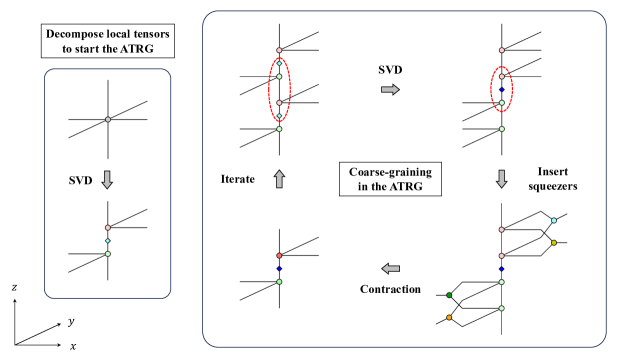
Figure 1: The decomposition of the initial tensor (left) and schematic overview of the ATRG algorithm (right) as proposed in Ref. [7].

The ATRG uses a decomposition of the initial tensor given by,

$$T_{(r_{1}m_{1}n_{1})(r_{2}m_{2}n_{2})(r_{3}m_{3}n_{3})(r_{4}m_{4}n_{4})(r_{5}m_{5}n_{5})(r_{6}m_{6}n_{6})}$$

$$\approx\sum_{\gamma}U_{(r_{1}m_{1}n_{1})(r_{2}m_{2}n_{2})(r_{3}m_{3}n_{3})\gamma}\sigma_{\gamma}V^{*}_{(r_{4}m_{4}n_{4})(r_{5}m_{5}n_{5})(r_{6}m_{6}n_{6})\gamma}$$ (6)

which can be seen in the left-hand side of Fig. 1. This initial singular value decomposition (SVD) of the tensor is used in the main updating step of the algorithm, as can be seen in the right-hand side of Fig. 1. The top and bottom of adjacent tensors are swapped via SVD in the algorithm, which allows for an algorithm that can be iterated.

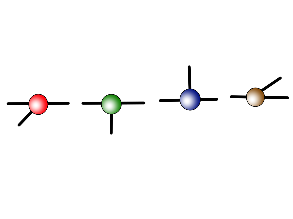
(a) An illustration of the decomposition of the initial tensors using triads.

(b) The higher-order tensor renormalization group [2] update applied to the tTRG.

Figure 2: Schematic picture of tTRG algorithm [4].

The tTRG uses a decomposition of the initial tensor into four smaller tensors. This decomposition can be approximate.

$$T_{ijklmn}=\sum_{a,b,c}A_{ika}B_{amb}C_{bnc}D_{clj}$$ (7)

Figure 2(a) gives an illustration of the four tensors and their connectivity. In the case of the $SU(2)$ PCM, the four tensors are given by

$$A_{\left(r_{1},m_{1},n_{1}\right)\left(r_{2},m_{2},n_{2}\right)(R,M,N)}=\sqrt{F_{r_{1}}(\beta)F_{r_{2}}(\beta)}C_{r_{1}m_{1}r_{2}m_{2}}^{RM}C_{r_{1}n_{1}r_{2}n_{2}}^{RN}$$ (8)

$$B_{(R,M,N)\left(r_{3},m_{3},n_{3}\right)\left(R^{\prime},M^{\prime},N^{\prime}\right)}=\frac{1}{\sqrt{d_{R^{\prime}}}}\sqrt{F_{r_{3}}(\beta)}C_{RMr_{3}m_{3}}^{R^{\prime}M^{\prime}}C_{RNr_{3}n_{3}}^{R^{\prime}N^{\prime}}$$ (9)

$$C_{\left(R^{\prime},M^{\prime},N^{\prime}\right)\left(r_{4},m_{4},n_{4}\right)\left(R^{\prime\prime},M^{\prime\prime},N^{\prime\prime}\right)}=\frac{1}{\sqrt{d_{R^{\prime}}}}\sqrt{F_{r_{4}}(\beta)}C_{R^{\prime\prime}M^{\prime\prime}r_{4}m_{4}}^{R^{\prime}M^{\prime}}C_{R^{\prime\prime}N^{\prime\prime}r_{4}n_{4}}^{R^{\prime}N^{\prime}}$$ (10)

$$D_{\left(R^{\prime\prime},M^{\prime\prime},N^{\prime\prime}\right)\left(r_{5},m_{5},n_{5}\right)\left(r_{6},m_{6},n_{6}\right)}=\sqrt{F_{r_{5}}(\beta)F_{r_{6}}(\beta)}C_{r_{5}m_{5}r_{6}m_{6}}^{R^{\prime\prime}M^{\prime\prime}}C_{r_{5}n_{5}r_{6}n_{6}}^{R^{\prime\prime}N^{\prime\prime}},$$ (11)

where the $C$s are Clebsch-Gordon coefficients, and $d_{r}$ is the dimension of the irrep. The algorithm updates the tensors iteratively using the HOTRG algorithm, and the update step can be seen in Fig. 2(b).

3 Observables & Results

To compare the tTRG and the ATRG we compare several observables. A simple quantity to extract from most tensor network algorithms is the free energy density given by (up to a sign),

$$F\equiv\frac{1}{V}\log(Z),$$ (12)

where $Z$ is the partition function, and $V$ is the system volume. The average action and its susceptibility are given by,

$$\langle s\rangle=\frac{\langle S\rangle}{V}\equiv-\frac{\partial}{\partial\beta}F,\quad\chi_{s}=V(\langle s^{2}\rangle-\langle s\rangle^{2})\equiv\frac{\partial^{2}}{\partial\beta^{2}}F.$$ (13)

Another useful observable first proposed in Ref. [12] which effectively counts the ground state degeneracy is defined as:

$$X\equiv\frac{\left(T_{aabbcc}\right)^{2}}{T_{abccdd}T_{baeeff}},$$ (14)

where the tensor indices are ordered left, right, front, back, top, bottom, and repeated indices are summed. This quantity can be computed in each direction during the update step in the tensor algorithm.

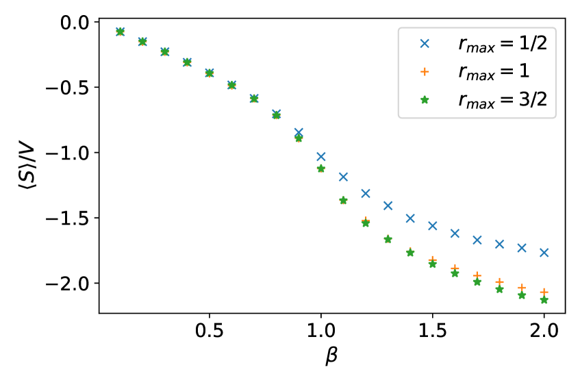
(a) ATRG, $D=40$, $V=1024^{3}$.

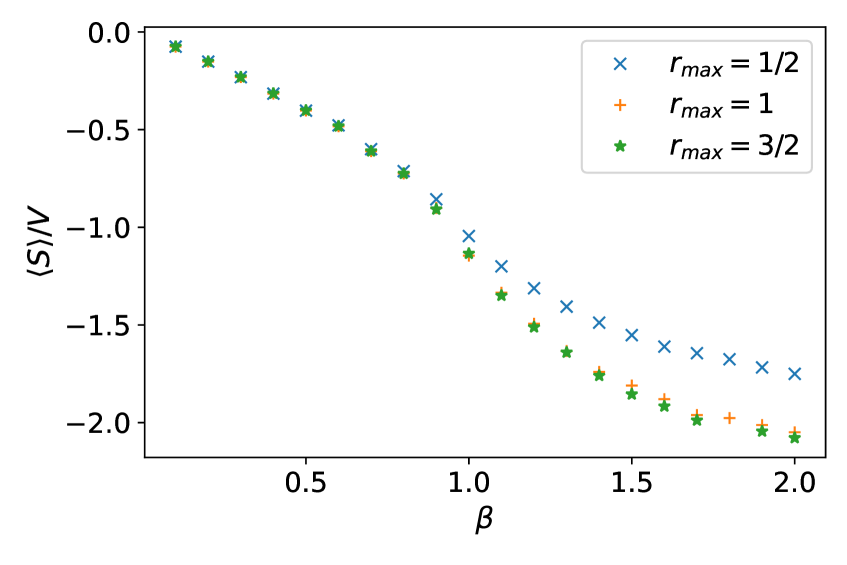
(b) Triad, $D=40$, $V=1024^{3}$.

Figure 3: Average action varying $r_{\rm max}$.

The results for the average action using ATRG and tTRG are shown in Figs. 3(a) and 3(b) for three different truncations across a range of $\beta$ values. These calculations were done at $V=1024^{3}$ with $D=40$.

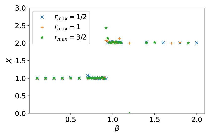
(a) Triad, $X$ varying $r_{\text{max}}$ and $\beta_{c}$, $D=40$, $V=1024^{3}$.
$r_{\text{max}}=1/2$: $\beta_{c}=0.935(5)$, $r_{\text{max}}=1$: $\beta_{c}=0.915(5)$, $r_{\text{max}}=3/2$: $\beta_{c}=0.915(5)$

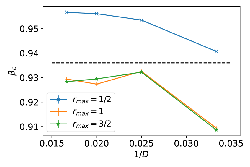
(b) $\beta_{c}$ from ATRG using $X$, $V=1024^{3}$. The recent MC estimation is $\beta_{c}=0.9360(1)$ [13] shown by the dashed line.

Figure 4: Estimation of the critical coupling using $X$ defined in (14)

.

To locate the phase transition in tensor computations, one usually has to compute the derivative of some observable. However, using $X$, we can locate transitions without explicitly computing any derivative. This is computationally easier. We computed $\beta_{c}$ using the discontinuous behavior of the observable, $X$. The result is shown in Fig. 4(a) using the tTRG for three different values of the irrep. cut-off. We find the critical coupling for $r_{\text{max}}=1/2$ differs from the next two highest cut-offs. Figure 4(b) shows similar results obtained using the ATRG. In this case, the results are shown as a function of the inverse tensor network bond dimension for the same three values of truncation. The convergence of $X$ as a function of the iteration step of the tTRG can be seen in Fig. 5. For sufficiently small $\beta$, $X$ converges to 1, while for large $\beta$ it converges to 2.

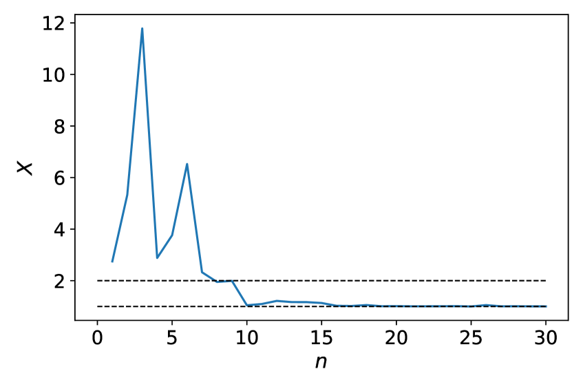
(a) $\beta=0.8$, $r_{\rm max}=1/2$

(b) $\beta=0.8$, $r_{\rm max}=1$

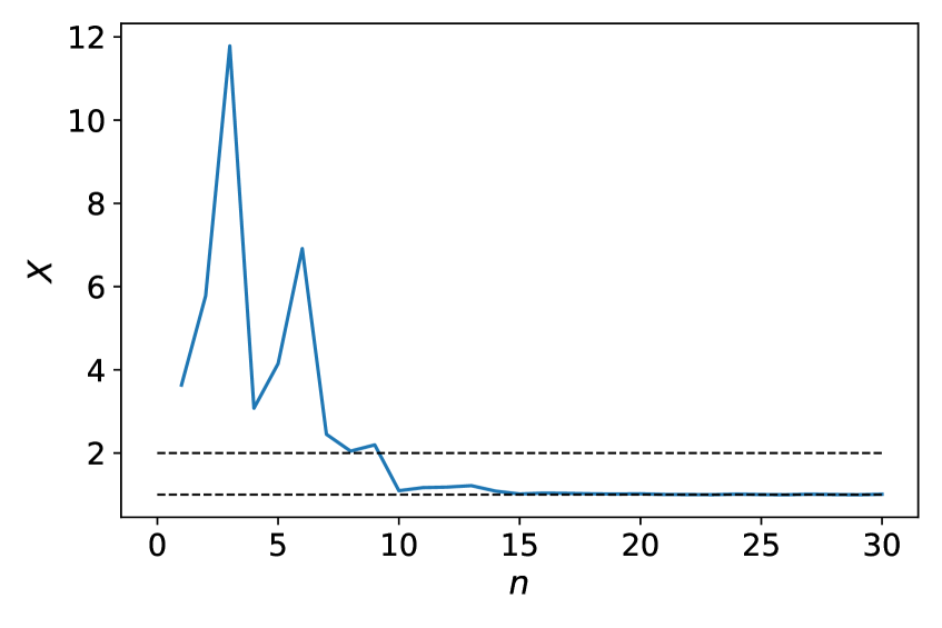
(c) $\beta=0.8$, $r_{\rm max}=3/2$

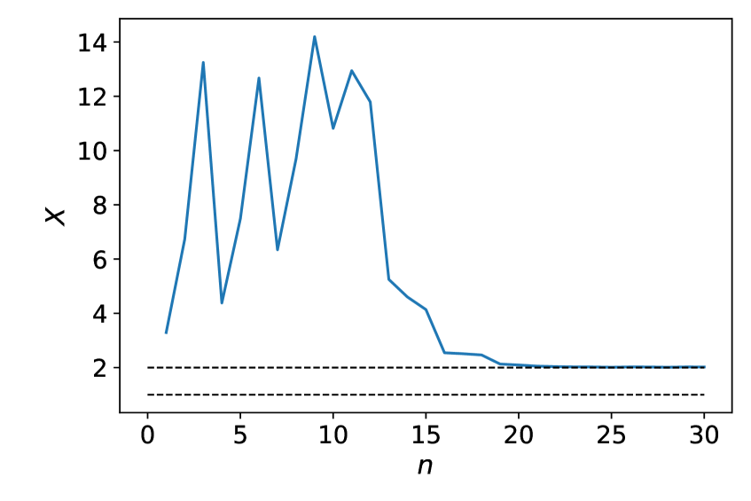
(d) $\beta=1.1$, $r_{\rm max}=1/2$

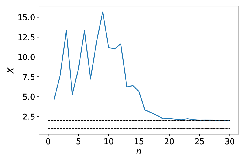
(e) $\beta=1.1$, $r_{\rm max}=1$

(f) $\beta=1.1$, $r_{\rm max}=3/2$

Figure 5: The convergence of $X$ with the number of coarse-graining step $n$, for two different $\beta$ values, and three different truncations.

Using the data for the average action, along with the results from calculating $X$, it is possible to extract a critical exponent $\alpha$ using the fitting ansatz

$$\langle S\rangle/V=A +B|\beta-\beta_{c}|+C|\beta-\beta_{c}|^{1-\alpha}.$$ (15)

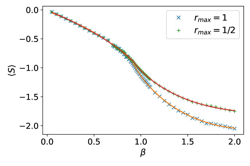
(a) Triad low-high temp fit, $D=40$, $V=1024^{3}$.
$r_{\rm max}=1/2$: $\beta_{c}=0.933(1)$, $r_{\rm max}=1$: $\beta_{c}=0.9232(1)$, $r_{\rm max}=3/2$: $\beta_{c}=0.92295(4)$

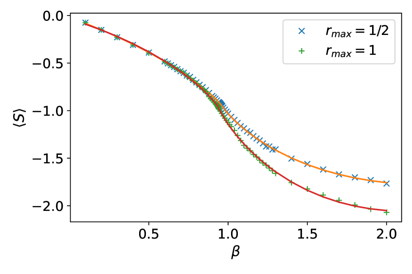
(b) ATRG low-high temp fit, $D=40$, $V=1024^{3}$.
$r_{\text{max}}=1/2$: $\alpha=-0.21259(1)$, $r_{\text{max}}=1$: $\alpha=-0.2151(1)$, $r_{\text{max}}=3/2$: $\alpha=-0.22676(4)$

Figure 6: Fitting the ansatz of (15) for the average action to the numerical results obtained from tTRG and ATRG at fixed bond dimension and lattice volume.

Figures 6(a) and  6(b) show results from fitting the above ansatz to the data. In the case of the tTRG, we first fix the value of $\alpha$ using the literature, $\alpha=-0.247(6)$ [14], then fit for $\beta_{c}$. The results in Fig. 6(a) are to be compared with the value $\beta_{c}=0.9360(1)$ [13]. For the ATRG we use the results from $X$ for the value of $\beta_{c}$ and fit to $\alpha$. In comparison to the calculation of $X$, again we find both with the tTRG and the ATRG that the $r_{\text{max}}=1/2$ case differs from the higher cut-off cases.

4 Conclusion

In our study, we find that both tTRG and the ATRG can be useful. The ATRG is more accurate at a fixed bond dimension, however, it is also computationally more expensive. Both methods seem to locate the phase transition reasonably well. In addition, our results show for the first time that the identification of the phase transition using $X$ which had only been used for models with discrete groups can be extended to models with continuous symmetry. The results from $X$ seem to indicate the transition is associated with a $\mathbb{Z}_{2}$ symmetry. To understand this better it would be interesting to calculate $\langle\text{Tr}\left[U\right]\rangle$ and its susceptibility. In addition, studying the $SU(3)$ PCM would increase the complexity of the model allowing a study of the group $SU(3)$ and its character expansion, which is crucial for later work on quantum chromodynamics. We leave these questions for future explorations.

References

- [1] M. Hauru, C. Delcamp, and S. Mizera, “Renormalization of tensor networks using graph-independent local truncations,” Phys. Rev. B 97 (Jan, 2018) 045111. https://link.aps.org/doi/10.1103/PhysRevB.97.045111.
- [2] Z. Y. Xie, J. Chen, M. P. Qin, J. W. Zhu, L. P. Yang, and T. Xiang, “Coarse-graining renormalization by higher-order singular value decomposition,” Phys. Rev. B 86 (Jul, 2012) 045139. https://link.aps.org/doi/10.1103/PhysRevB.86.045139.
- [3] F. Verstraete and J. I. Cirac, “Renormalization algorithms for quantum-many body systems in two and higher dimensions,” 2004.
- [4] D. Kadoh and K. Nakayama, “Renormalization group on a triad network,” 2019.
- [5] Y.-Y. Shi, L.-M. Duan, and G. Vidal, “Classical simulation of quantum many-body systems with a tree tensor network,” Phys. Rev. A 74 (Aug, 2006) 022320. https://link.aps.org/doi/10.1103/PhysRevA.74.022320.
- [6] M. Gerster, P. Silvi, M. Rizzi, R. Fazio, T. Calarco, and S. Montangero, “Unconstrained tree tensor network: An adaptive gauge picture for enhanced performance,” Phys. Rev. B 90 (Sep, 2014) 125154. https://link.aps.org/doi/10.1103/PhysRevB.90.125154.
- [7] D. Adachi, T. Okubo, and S. Todo, “Anisotropic tensor renormalization group,” Phys. Rev. B 102 (Aug, 2020) 054432. https://link.aps.org/doi/10.1103/PhysRevB.102.054432.
- [8] L. Susskind, “Lattice models of quark confinement at high temperature,” Phys. Rev. D 20 (Nov, 1979) 2610–2618. https://link.aps.org/doi/10.1103/PhysRevD.20.2610.
- [9] R. D. Pisarski and F. Wilczek, “Remarks on the chiral phase transition in chromodynamics,” Phys. Rev. D 29 (Jan, 1984) 338–341. https://link.aps.org/doi/10.1103/PhysRevD.29.338.
- [10] D. Toussaint, “Scaling functions for o(4) in three dimensions,” Phys. Rev. D 55 (Jan, 1997) 362–366. https://link.aps.org/doi/10.1103/PhysRevD.55.362.
- [11] C. Bernard, C. DeTar, S. Gottlieb, U. M. Heller, J. Hetrick, K. Rummukainen, R. L. Sugar, and D. Toussaint, “Critical behavior in staggered fermion thermodynamics,” Phys. Rev. D 61 (Jan, 2000) 054503. https://link.aps.org/doi/10.1103/PhysRevD.61.054503.
- [12] Z.-C. Gu and X.-G. Wen, “Tensor-entanglement-filtering renormalization approach and symmetry-protected topological order,” Phys. Rev. B 80 (Oct, 2009) 155131. https://link.aps.org/doi/10.1103/PhysRevB.80.155131.
- [13] E. López-Contreras, J. A. García-Hernández, E. N. Polanco-Euán, and W. Bietenholz, “The 3d o(4) model as an effective approach to the QCD phase diagram,” Suplemento de la Revista Mexicana de Física 3 no. 2, (Jun, 2022) . https://doi.org/10.31349%2Fsuplrevmexfis.3.020727.
- [14] F. P. Toldin, A. Pelissetto, and E. Vicari, “The scaling equation of state of the 3-d o(4) universality class,” Journal of High Energy Physics 2003 no. 07, (Jul, 2003) 029. https://dx.doi.org/10.1088/1126-6708/2003/07/029.