Experiment-Informed Finite-Strain Inverse Design of Spinodal Metamaterials

Abstract

This study presents a novel physics-enhanced machine learning (ML) and optimization framework tailored to address the challenges of designing intricate spinodal metamaterials with customized mechanical properties in scenarios where computational modeling is restricted, and experimental data is sparse. By utilizing sparse experimental data directly, our approach facilitates the inverse design of spinodal structures with precise finite-strain mechanical responses. Leveraging physics-based inductive biases to compensate for limited data availability, the framework sheds light on instability-induced pattern formation in periodic metamaterials, attributing it to nonconvex energetic potentials. Inspired by phase transformation modeling, the method integrates multiple partial input convex neural networks to create nonconvex potentials, effectively capturing complex nonlinear stress-strain behavior, even under extreme deformations.

Introduction

The rapid advancement of resolution and throughput in additive manufacturing has opened doors to new possibilities in engineering mechanical metamaterials (or architected materials) with properties that were once unattainable using conventional manufacturing techniques [1, 2, 3, 4, 5]. These properties include, e.g., high strength-to-weight ratios [6, 2], negative Poisson’s ratios [7], mechanical cloaking abilities [8], tailorable anisotropic stiffnesses [9, 10, 11, 12], and high energy absorption [13, 14]. While explorations on mechanical metamaterials have primarily focused on periodic and symmetric truss-[15] and plate[16]-based lattices, recently more attention has been given to shell-based morphologies. These morphologies, such as triply periodic minimal surfaces [17, 18] and spinodal architectures [9, 19, 20, 21] have gained traction in the field as they do not possess nodes or joints, behave in a mechanically efficient manner due to their doubly curved shells, and inherently mitigate stress concentrations.

Spinodal-like—or spinodoid—metamaterials are especially intriguing because they possess an aperiodic and asymmetric microstructure resembling the morphologies observed during the early stages of spinodal decomposition or rapid diffusion-driven phase separation in a homogeneous mixture of immiscible phases (Figure 1). These nature-inspired designs spanning multiple length scales—from nanoscale to macroscale—can either be manufactured using scalable self-assembly via polymerization-induced phase separation in polymer blends[19] or additive manufacturing of morphologies extracted from phase separation simulations[20, 21]. In contrast to truss-, plate- and shell-based lattices, the resulting smooth and bicontinuous topologies enable robustness to manufacturing defects, mitigate any harmful stress concentrations, and exhibit extreme mechanical resilience[19, 21]. In silico tuning of the underlying energetics of the spinodal decomposition process opens up a diverse design space of topologies and corresponding mechanical properties[20, 9, 22], leading to a recent flurry of proposed spinodal metamaterials for ultralight structures[23, 24, 19, 25], energy absorption[26, 27, 21], bone-mimetic implants[9, 28], acoustics[29], mass transport[30], among other applications.

Despite the recent advances, the structure-property relations of spinodal metamaterials have primarily been explored only in a forward fashion—computational or experimental mechanical analyses of a few representative samples chosen through trial-and-error or intuition of the design space[23, 24, 19, 26, 27, 21, 31]. Furthermore, clear links between specific features of the morphology and the ensuing mechanical response are lacking. In light of the vast design space of spinodal metamaterials, the question of interest is that of inverse design, i.e., how to efficiently identify designs with tailored properties dictated by stress-strain responses. While machine learning (ML) has recently seen some success in inverse design of metamaterials[9, 24, 12, 10, 22, 32, 33, 11, 34, 35, 36, 37, 38]—including but not limited to spinodal metamaterials—these algorithms face a challenge of quality-quantity duality.

High-throughput simulations of mechanical responses yield large quantities of data, which are of sufficient fidelity only in linear and small-strain regimes. For instance, in the context of spinodal metamaterials, ML models have been trained on in silico data to inversely design for linear stiffness tensor components and tailored anisotropy[9]. However, in the case of finite-strain behaviors, responses due to phenomena such as material and geometric nonlinearities, buckling, self-contact, dissipation, fracture, and meshing artifacts add significant complexity and computational cost. On the contrary, while experimental data can serve as the ground-truth, highest-fidelity data for ML models, the quantity of data is severely limited by the number of time-consuming and costly experiments that can be reasonably performed.

Here, we propose a direct experiment-to-ML inverse design framework to design spinodal metamaterials with tailored finite-strain mechanical responses. We create a small but reasonably sized dataset of 107 shell-based spinodal metamaterial architectures along with their stress-strain responses to 40% strain—obtained experimentally via ex situ and in situ nanomechanical uniaxial compression along three principal directions. The ML framework consists of a forward model that surrogates the structure-to-property relations and an inverse optimization scheme that finds the designs for a target large-deformation stress-strain response. To address the quality-quantity duality challenge, we introduce a new ML architecture that uses physics-enhanced inductive biases to eliminate the need for large-quantity and low-quality simulations data. Despite the limited amount of data, we successfully predict the finite-strain response including energy absorption estimates up to 40% strain for various spinodal morphologies. Furthermore, given a target stress-strain curve that lies outside the training data domain, the framework can efficiently identify a spinodal morphology that exhibits the target behavior. Altogether, this experiment-informed ML effort closes the gap between the structure-property relations of spinodal metamaterials, particularly by going into nonlinear responses while accounting for physics-based deformation mechanisms in complex architectures.

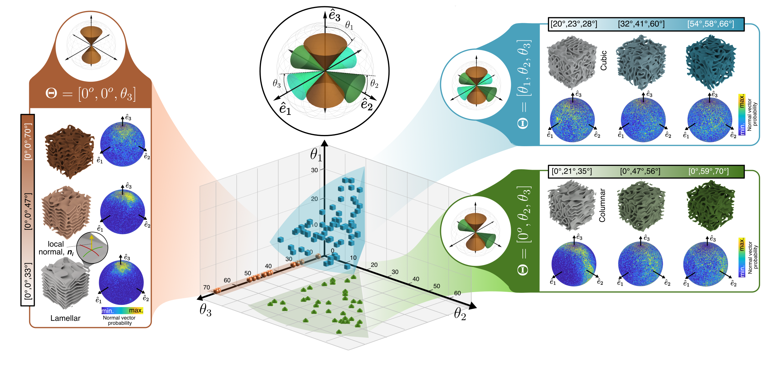
Figure 1: Spinodal morphology design space defined by a three-parameter $\bm{\Theta}$ representation (center). Three design subspaces, defined by the non-zero dimensionality of the $\bm{\Theta}=[\theta_{1},\theta_{2},\theta_{3}]$ vector are represented by color clouds encompassing the designs used for training. The one-dimensional (1D) subspace corresponding to lamellar morphologies was represented by a non-zero $\theta_{3}$, while the 2D and 3D subspaces subsequently added non-zero $\theta_{2}$ and $\theta_{3}$ parameters and corresponded to columnar and cubic morphologies, respectively. Three representative designs of increasing norm $|\bm{\Theta}|$ are presented within each subspace, along with pole figures denoting the directional probability of normal vectors $\bm{n}$.

Spinodal morphology design space

To replicate a variety of morphologies obtained through spinodal decomposition, such as those obtained in diffusion-driven phase separation of a homogeneous mixture of immiscible phases, our first step is to define a design space that parametrizes all possible morphologies. Cahn [39] demonstrated that the resulting phase field solution to the canonical Cahn-Hilliard equation can be approximated by a Gaussian random field (GRF), i.e., a superposition of a large number of standing waves with a narrow band of similar wavenumbers. In Fourier space, this corresponds to a spectral density function (SDF) given by a diffused spherical surface of radius equal to the wavenumber (denoted by $\beta$ henceforth) and centered at the origin. Inspired from the formalization of this approximation[30, 40], we construct the phase field $\varphi:\Omega\rightarrow\mathbb{R}$ in a domain $\Omega\subset\mathbb{R}^{3}$ directly in Fourier space as

$$\varphi=\mathcal{F}^{-1}\bigg{[}\mathcal{F}[\varphi_{\text{noise}}]\odot\mathcal{F}[\varphi_{\text{filter}}]\bigg{]}=\mathcal{F}^{-1}\bigg{[}\mathcal{F}[\varphi_{\text{noise}}]\odot\left({\rho[\varphi_{\text{filter}}]}\right)^{1/2}\bigg{]}.$$ (1)

Here, $\mathcal{F}[\cdot]$, $\mathcal{F}[\cdot]^{-1}$, and $\rho[\cdot]$ denote the Fourier transform, inverse Fourier transform, and SDF (squared magnitude of the Fourier transform), respectively, while $\odot$ denotes the Hadamard product, $\varphi_{\text{noise}}$ represents the initial phase field of a homogeneous mixture of immiscible phases as an independent and identically distributed standard Gaussian noise (i.e., zero mean and unit variance). Convolution of $\varphi_{\text{noise}}$ with $\varphi_{\text{filter}}$ (equivalently, Hadamard product in the Fourier space) represents the phase separation process that transforms the homogeneous mixture $\varphi_{\text{noise}}$ into the phase-separated phase field $\varphi$. We define $\varphi_{\text{filter}}$ through its SDF as

$$\rho[\varphi_{\text{filter}}](\bm{k}) =\underbrace{\exp\left(-\frac{(r-\beta)^{2}}{2\lambda_{r}^{2}}\right)}_{\text{wavenumber control}}\odot\underbrace{\sum_{i=1}^{3}\sigma\left(-\lambda_{\phi}(\phi_{i}-\theta_{i})\right)}_{\text{anisotropy control}}$$ (2)

$$\text{with}\qquad\phi_{i}=\min\{\cos^{-1}(k_{i}/r),-\cos^{-1}(k_{i}/r)\}\quad\text{and}\quad r=\|\bm{k}\|,$$

where $\bm{k}$ denotes a wave-vector in the Fourier space; with $\lambda_{r}>0$ and $\lambda_{\phi}>0$ as constants. The first term—labeled wavenumber control—specifies that the spectral density is limited to a narrow Gaussian band with mean wavenumber $\beta$ and standard deviation $\lambda_{r}$. Choosing a higher $\beta$ yields morphologies with a finer microstructural lengthscale. The second term—labeled anisotropy control—adds directional constraints to the wave-vectors. Specifically, the wave-vectors’ orientations (given by $\phi_{i}$) are constrained to cones centered at the origin and along the principal axes $\{\hat{\bm{e}}_{1},\hat{\bm{e}}_{2},\hat{\bm{e}}_{3}\}$ with half-angles $\{\theta_{1},\theta_{2},\theta_{3}\}$, respectively (Figure 1, center). However, instead of a hard limit, we relax the constraint by using a smooth sigmoid-type function, which in this case is $\sigma(\cdot)=(1+\tanh(\cdot))/2$. Consequently, the probability of a wave-vector outside the cones decreases fast but smoothly with the rate determined by $\lambda_{\phi}$. We add both radial and angular smoothing in the SDF to mitigate formation of non-smooth artifacts in the generated morphology. We highlight that this model of anisotropy control is not just a mathematical construct; rather it serves as an approximation to the canonical Cahn-Hilliard equation with anisotropic mobility[9].

Choosing a cubic domain $\Omega$ of size $\ell\times\ell\times\ell$, the Fourier transforms in Eq. (1) are performed on a uniform grid of $\Omega$ with $K\times K\times K$ resolution, automatically ensuring triple periodicity in the generated structure. The morphology of the spinodal metamaterial is obtained by computing the zero level-set of $\varphi$, i.e., for $\bm{x}\in\Omega$, followed by extruding the surface pointwise along both inward and outward normal directions equally for a final surface thickness of $h\ll\ell$. Note that due to the randomness of $\varphi_{\text{noise}}$, the resulting structures are stochastic and hence two morphology realizations for the same design parameters may be different. To reduce the effects of stochasticity, we choose $\beta\ell$ and $h/\ell$ to be sufficiently high and low, respectively, to ensure separation of scales between the microstructural length scale and the domain dimensions. We validate the choice in $\beta$ and $h$ through a systematic computational homogenization analysis as well as manufacturing considerations, respectively (Supplementary Information Section 2.1).

For the scope of this work, we uniquely defined each spinodal metamaterial design by the design parameters $\bm{\Theta}=[\theta_{1},\theta_{2},\theta_{3}]$ with $\theta_{1},\theta_{2},\theta_{3}\in\{0\}\cup[\theta_{\text{min}},\theta_{\text{max}}]$ (i.e., the cone angles), while keeping the remaining parameters constant (see Supplementary Information Table 1). The angles, when non-zero, are lower-bounded by $\theta_{\text{min}}=20^{\circ}$ to ensure bi-continuity of the structures[9] and upper-bounded by $\theta_{\text{max}}=70^{\circ}$ to avoid degenerate (almost) isotropic structures. For instance, when $\bm{\Theta}=[0,0,\theta_{3}]$, this one-dimensional (1D) parameter subspace results in structures with distinctive lamellar-like features (Figure 1, left). In contrast, the corresponding 2D and 3D parameter subspaces—$\bm{\Theta}=[0,\theta_{2},\theta_{3}]$ and $\bm{\Theta}=[\theta_{1},\theta_{2},\theta_{3}]$—exhibit columnar- or cubic-like features, respectively (Figure 1, right). The resulting morphologies can be characterized by their corresponding surface-normal distributions, represented as spherical pole figures in Figure 1, indicating the directional distribution of material curvature within the morphologies. Overall, the design space admits a large and diverse set of morphological anisotropy, with the aim of linking said structures to their unique mechanical responses.

Notably, increases in the magnitudes of the $\theta_{i}$ parameters, approaching the theoretical maximum of $90^{\circ}$, results in isotropically distributed wave-vectors and the anisotropic structural distinctions disappear. However, for the sake of clarity in the subsequent discussions, we use the terminology of lamellar, columnar, and cubic structures when referring to the 1D, 2D, and 3D subspaces of $\bm{\Theta}$, respectively, regardless of their absolute values.

Dataset generation via nanomechanical experiments

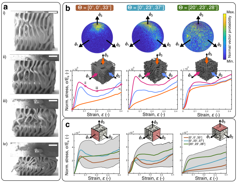
Figure 2: (a) In situ snapshots $i$–$iv$ showing the progression of deformation for the $\bm{\Theta}=[0^{\circ},0^{\circ},33^{\circ}]$ morphology along the $\hat{\bm{e}}_{1}$ direction, up to 40% strain. Scale bars, 20 µm. (b) Qualitative structure-to-response relations enabled by spherical pole figures denoting the directional surface-normal distributions for representative lamellar (left), columnar (center), and cubic (right) morphologies—accompanied by corresponding stress-strain responses along the $\hat{\bm{e}}_{i}$ directions. The pole figures serve as a proxy for structural anisotropy, with higher surface-normal distributions along a given direction correlating to a more compliant response. The lamellar and columnar morphologies exhibited negative-stiffness regions corresponding to nonlinear buckling (as marked for the lamellar sample shown in (a)), along with stiffening at large deformations due to self-contact of shells. (c) Range of finite stress-strain behaviors across the training data as observed from ex situ compressions along the three principal directions $\hat{\bm{e}}_{1}$ (left), $\hat{\bm{e}}_{2}$ (center), $\hat{\bm{e}}_{3}$ (right) highlighted on a generic spinodal morphology. The black lines denote the stress bounds across the training dataset, while color-coded responses correspond to the three representative morphologies shown in (b).

Sampling from the design space defined above, we generated a small dataset consisting of $N=107$ spinodal morphologies by randomly sampling $\bm{\Theta}$. The dataset included 11 lamellar ($\bm{\Theta}=[0,0,\theta_{3}]$), 36 columnar ($\bm{\Theta}=[0,\theta_{2},\theta_{3}]$), and 60 cubic ($\bm{\Theta}=[\theta_{1},\theta_{2},\theta_{3}]$, with $\theta_{1}<\theta_{2}<\theta_{3}$) morphologies. To augment our experimental effort, we removed redundancy in data generation due to permutation symmetry in the parameterization (e.g., the response along $\hat{\bm{e}}_{1}$ for $[\theta_{1},\theta_{2},\theta_{3}]$ is equivalent to the response along $\hat{\bm{e}}_{2}$ for $[\theta_{2},\theta_{1},\theta_{3}]$). To determine the response along the 3 principal directions for each of the $N$ morphologies, we fabricated 321 samples, corresponding to 609 effective $\bm{\Theta}$ parametrizations within our design space due to permutation symmetry (see Supplementary Information Section 1). The 321 samples were fabricated out of IP-Dip photoresist using a two-photon lithography process (Materials and Methods), resulting in cubic unit cells with an average edge length of $\ell=92$ µm and shell thickness of $h=2.6$ µm, with an approximate relative density (i.e., fill fraction) of 40%.

To obtain the finite-strain response of each sample in the dataset, we performed both ex situ and in situ quasi-static uniaxial compression experiments (strain rate of $10^{-3}$ s^-1) along the three principal directions $\hat{\bm{e}}_{1}$, $\hat{\bm{e}}_{2}$, and $\hat{\bm{e}}_{3}$. In situ observation of the compression enabled visualization of multiple nonlinear and irreversible mechanisms such as plastic buckling, self-contact, and fracture through the thickness of the shells (Figure 2a)—which could be linked to specific characteristics of the large-deformation stress-strain response. The loading portion of the measured 321 stress-strain curves were used to train the ML model for inverse design, while the unloading portion was omitted since it carried minimal information in this large-strain regime (full loading-unloading responses are presented in Supplementary Information Section 2.3). To facilitate comparison to spinodal metamaterials made of similar polymeric constituents, we report the stress normalized by the elastic modulus $E_{s}$ of IP-Dip photoresist.

As an appropriate qualitative indicator of mechanical anisotropy within each design, we represented the surface normal distributions in the form of a spherical pole figure, indicating relative orientation of curved shells with respect to a loading direction (Figure 2b). Regions with a higher distribution of surface normals correlated to a more compliant response in the linear regime, followed by an on-average lower stress level throughout subsequent deformation. In the cases of lamellar and columnar morphologies, directions with low surface-normal distributions tended to exhibit plastic buckling beyond the onset of nonlinearity (at strains of $\varepsilon\approx 5\%$) and consequently, negative-stiffness responses up to strains of $\varepsilon\approx 20\%$ as observed via in situ experiments on the $\bm{\Theta}=[0^{\circ},0^{\circ},33^{\circ}]$ morphology (Figure 2a,b left). Notably, the cubic morphologies approach similar responses when loading in all three directions with $\theta_{1}\approx\theta_{2}\approx\theta_{3}$. Further in situ observations for the representative samples are presented in Figure 2b, are found in the Supplementary Information Section 2.3.

When analyzing the dataset as a whole—simply represented in Figure 2c as bounded by maximum and minimum responses with some highlighted morphologies within—we identify the buckling behavior to be prevalent in other lamellar morphologies as well as some low-angle columnar morphologies (i.e., when $\theta_{2}<30^{\circ}$). For the subset of fabricated samples, we identified a distinctively different response in $\hat{\bm{e}}_{3}$-loaded responses, primarily exhibiting monotonically increasing stress levels—a consequence of our $\theta_{1}<\theta_{2}<\theta_{3}$ criterion when selecting morphologies. We highlight that between the strains of $\varepsilon\approx 20\%$ to 40%, micro-cracks began to form causing fracture events that manifested as fluctuations in the stress response. Defining the energy absorbed as the integral of the stress-strain responses to 40% strain provided a broad distribution of performance metrics as a function of morphology and orientation.

Altogether, this comprehensive dataset sheds light on the complex normal distribution-to-response relations in high relative density spinodal morphologies, adding mechanics-based intuition to a previously obscure concept[19, 21]. However, we note that this added intuition falls short beyond the moderate-deformation regime, necessitating the use of high-fidelity computational tools or ML models to reliably predict responses such as those emanating from self-contact or nonlinear buckling.

Forward modeling via physics-enhanced deep learning

Learning the highly nonlinear map from the design parameters $\bm{\Theta}$ to the direction-dependent stress-strain responses of spinodal metamaterials would require a significant amount of data. To circumvent this issue and to work with limited experimental data available, we introduce a physics-enhanced ML framework that serves as a surrogate to the forward structure-to-property relations.

In the exemplar stress-strain behaviors in Figure 2b, we observe nonlinear features that are typical of instabilities and pattern formation in bulk materials due to nonconvex energetics[41]. Therefore, we model a representative stress-strain response as the derivative of an underlying strain energy density potential, which in the context of uniaxial compression corresponds to the area under the stress-strain curve. Consequently, the potential as a function of the applied strain must be monotonically increasing while admitting nonconvexities to allow for instabilities. We emphasize that this notion of energy potential is used only as an inductive bias to facilitate the learning of the uniaxial stress-strain response; its physical and thermodynamical admissibility should not be considered as strictly as a homogenized constitutive model.

We model the above potential with a deep neural network (NN) $W(\varepsilon,\bm{\Theta})$ as a function of the applied strain $\varepsilon$ and design parameters $\bm{\Theta}$. A classical NN based on, e.g., a multi-layer perceptron (MLP) architecture may not satisfy the constraint of monotonic increase with $\varepsilon$. Additionally, while such an NN is highly non-convex in its inputs by default, the degree of nonconvexity (loosely speaking) with respect to $\varepsilon$ should be constrained. The experimental data clearly exhibits a single macrostructural instability, which should be accordingly reflected in the NN output. Since we are training on experimental data directly, the NN—left unchecked—can exhibit fine-scale but highly oscillatory behavior trying to fit the experimental noise[42]. To satisfy the above constraints, we introduce the following NN architecture.

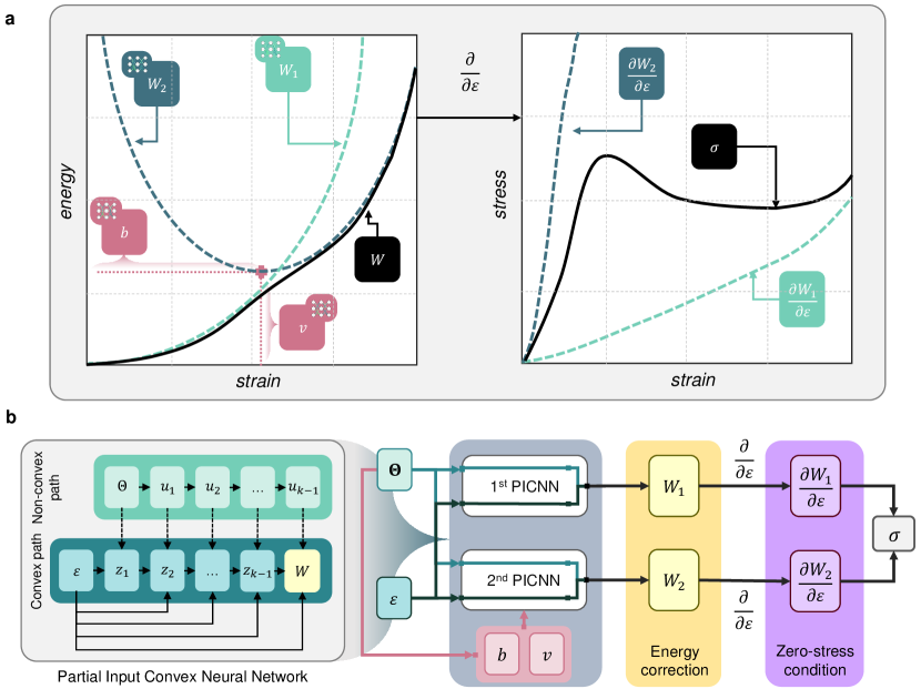
Figure 3: (a) Left: The uniaxial compression stress response (as a function of applied strain $\varepsilon$) of spinodal metamaterials is modeled as the derivative of a deep neural network-based nonconvex energy density potential $W(\varepsilon,\bm{\Theta})$. The model consists of two potentials convex in $\varepsilon$ and given by separate neural networks: $W_{1}(\varepsilon,\bm{\Theta})$ with the energy and stress vanishing at $\varepsilon=0$ by construction; $W_{2}(\varepsilon,\bm{\Theta})$ with the energy $(v+W_{1}(b,\bm{\Theta}))$ and vanishing stress at $\varepsilon=b$. Both $b(\bm{\Theta})$ and $v(\bm{\Theta})$ are also given by neural networks. The nonconvex potential $W$ is obtained by a combination of $W_{1}$ and $W_{2}$. Right: The stress is obtained by differentiating $W$ with respect to $\varepsilon$. Also shown are the derivatives of $W_{1}$ and $W_{2}$ for reference. (b) Schematic of the partial input convex neural network (PICNN) architecture for $W_{1}$ and $W_{2}$ and their combination thereof. The PICNN architecture predicts an energy which is convex with respect to the strain $\varepsilon$ (via convex path) and parameterized by the design parameters $\bm{\Theta}$ (via nonconvex path). See Supplementary Information Section 3.3 for details.

We take inspiration from Kumar et al.[41] and combine multiple convex potentials into one monotonically increasing, but nonconvex potential as

$$W(\varepsilon,\bm{\Theta})=\min\{W_{1}(\varepsilon,\bm{\Theta}),W_{2}(\varepsilon,\bm{\Theta})\},$$ (3)

where $W_{1}(\varepsilon,\bm{\Theta})$ and $W_{2}(\varepsilon,\bm{\Theta})$ are two energy potentials that are convex in $\varepsilon$ (but non-convex in $\bm{\Theta}$). However, the corresponding transition between phases is very sharp and not representative of the experimental data. Therefore, we relax Eq. (3) by allowing the phases to coexist with volume fractions $\gamma_{1},\gamma_{2}\in[0,1]$, respectively, as

$$W(\varepsilon,\bm{\Theta})=\min_{\gamma_{1},\gamma_{2}}\ \Bigg{[}\sum_{i=1}^{2}\gamma_{i}W_{i}(\varepsilon,\bm{\Theta})-\underbrace{\left(-k_{T}\sum_{i=1}^{2}\gamma_{i}\log\gamma_{i}\right)}_{\text{configurational entropy}}\Bigg{]},\qquad\text{with}\quad\gamma_{1}+\gamma_{2}=1.$$ (4)

Here, the configurational entropy (not physical entropy) penalizes the formation of phase mixtures. The constant $k_{T}>0$ controls the influence of configurational entropy and in turn, the smoothness of the transition between $W_{1}$ and $W_{2}$. The effective stress $\sigma$ is obtained as the derivative of $W(\varepsilon,\bm{\Theta})$

$$\sigma(\varepsilon,\bm{\Theta})=\frac{\partial W}{\partial\varepsilon}=\frac{\exp\left(-\frac{W_{1}}{k_{T}}\right)}{\exp\left(-\frac{W_{1}}{k_{T}}\right)+\exp\left(-\frac{W_{2}}{k_{T}}\right)}\frac{\partial W_{1}}{\partial\varepsilon}+\frac{\exp\left(-\frac{W_{2}}{k_{T}}\right)}{\exp\left(-\frac{W_{1}}{k_{T}}\right)+\exp\left(-\frac{W_{2}}{k_{T}}\right)}\frac{\partial W_{2}}{\partial\varepsilon},$$ (5)

where the simplification on the right side follows from the analytical solution of Eq. (4) (see Supplementary Information Section 3.2 for derivation).

We model the constituent potential $W_{1}$ as

$$W_{1}(\varepsilon,\bm{\Theta})=\underbrace{\mathcal{P}_{\omega_{1}}(\varepsilon,\bm{\Theta})}_{\text{first convex potential}}-\underbrace{\mathcal{P}_{\omega_{1}}(0,\bm{\Theta})}_{\text{energy correction}}-\underbrace{\varepsilon\frac{\partial\mathcal{P}_{\omega_{1}}(0,\bm{\Theta})}{\partial\varepsilon}}_{\text{stress correction}}.$$ (6)

Here, $\mathcal{P}_{\omega_{1}}$ denotes a partial input convex NN (PICNN) (see ref.[43] for architectural details) with the trainable parameter set $\omega_{1}$. Due to the inherent property of PICNNs, the predicted $W_{1}$ is modeled to be only convex with respect to ${\varepsilon}$, but can have any arbitrary functional relationships with $\bm{\Theta}$. We name these functional relationships within the PICNN architecture as the convex and nonconvex path (as seen in Figure 3b). Following the principle that non-negative weighted sums of convex functions are convex, the convex path only contains linear transformations with non-negative weights and convex and non-decreasing nonlinear activation functions. Supplementary Information Section 3.3 provides further details on the PICNN architecture used here. This PICNN-based approach allows us to obtain energies convex in $\varepsilon$ but non-convexly parameterized by $\bm{\Theta}$. The energy and stress correction terms ensure that $W_{1}$ identically satisfies zero energy and zero stress (strain-derivative of $W_{1}$) at zero strain, i.e., $\varepsilon=0$.

We model the constituent potential $W_{2}$ as

$$W_{2}(\varepsilon,\bm{\Theta}) =\underbrace{\mathcal{P}_{\omega_{2}}(\varepsilon-b,\bm{\Theta})}_{\text{second convex potential}}-\underbrace{\left(\mathcal{P}_{\omega_{2}}(0,\bm{\Theta})-v-W_{1}(b,\bm{\Theta})\right)}_{\text{energy correction}}-\underbrace{(\varepsilon-b)\frac{\partial\mathcal{P}_{\omega_{2}}(0,\bm{\Theta})}{\partial\varepsilon}}_{\text{stress correction}},$$ (7)

$$\text{with}\qquad b=\mathcal{F}_{\beta}(\bm{\Theta})\geq 0\qquad\text{and}\qquad v=\mathcal{F}_{\nu}(\bm{\Theta})\geq 0.$$

Here, $\mathcal{P}_{\omega_{2}}$ denotes another PICNN that is convex in $\varepsilon$ and contains trainable parameters $\omega_{2}$. However, unlike $W_{1}$, the energy and stress correction terms ensure that minimizer and minimum of $W_{2}$ are non-zero, i.e., $\varepsilon=b\geq 0$ and $W_{2}(b,\bm{\Theta})=v+W_{1}(b,\bm{\Theta})$. Both $b$ and $v$ act as offsets of $W_{2}$ with respect to $W_{1}$ in the strain vs. energy space. Their values are given by two additional classical MLP neural networks $\mathcal{F}_{\beta}(\bm{\Theta})$ and $\mathcal{F}_{\nu}(\bm{\Theta})$, parameterized by $\beta$ and $\nu$, respectively. The non-negativity constrain on $b$ and $v$ ensure that the non-convex combination of $W_{1}$ and $W_{2}$ in Eq. (4) yields a $W$ that is monotonically increasing (see Figure 3a).

We represent the experimentally generated dataset as

$$\mathcal{D}=\left\{\left(\bm{\Theta}^{(n)},\tilde{\epsilon}_{t}^{(n,i)},\tilde{\sigma}_{t}^{(n,i)}\right)\ :\ t=1,\dots,T{(n,i)};\ i=1,2,3;\ n=1,\dots,N\right\},$$ (8)

where $n$, $i$, and $t$ denote the different sample, direction of loading, and loadstep during loading, respectively. The total number of loadsteps $T(n,i)$ as well as change in strain between two loadsteps may not necessarily be the same across different samples and direction of loading. The forward ML model is then trained to minimize the mean absolute percentage error (MAPE) loss in stress predictions across the small training dataset:

$$\omega_{1},\omega_{2},\beta,\nu\ \leftarrow\ \operatorname*{arg\,min}_{\omega_{1},\omega_{2},\beta,\nu}\ \frac{1}{|\mathcal{D}|}\ \sum_{n=1}^{N}\ \sum_{i=1}^{3}\ \sum_{t=1}^{T(n,i)}\ \left|\frac{\sigma\left(\tilde{\varepsilon}_{t}^{(n,i)},\bm{\Theta}^{(n)}\right)-\tilde{\sigma}^{(n,i)}_{t}}{\tilde{\sigma}^{(n,i)}_{t}}\right|.$$ (9)

The loss function computes the relative error of the predicted and target values, ensuring that the predictions are forced to be accurate, regardless of the magnitude of the target value. Supplementary Information Section 3.4 presents the detailed ML training protocols.

Due to the limited amount of data, we take additional measures to facilitate the training process. For each data point, we distinguish between the type of spinodal topologies (lamellar, columnar, or cubic) and the loading directions ($\hat{\bm{e}}_{1},\hat{\bm{e}}_{2},$ and $\hat{\bm{e}}_{3}$). For each of these cases, we train distinct ML models and post-hoc lump them into a unified model; see Supplementary Information Section 3.4 for details.

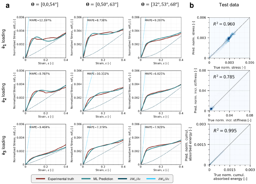
Figure 4: (a) Stress-strain plots showing the ML-predicted (teal) versus experimental ground truth (red) curves for three representative spinodal design in the test dataset (i.e., sample from outside the training dataset). For reference, we show the derivatives $\partial W_{1}/\partial\varepsilon$ (dark blue) and $\partial W_{2}/\partial\varepsilon$ (light blue). (b) Distribution of predicted vs. ground truth values on the test dataset for normalized stress, normalized incremental stiffness (i.e., slope of curve), and normalized cumulative energy absorbed (i.e., area under curve) at all strain increments. The dashed line represents the ideal line with zero intercept and unit slop; $R^{2}$ denotes the corresponding goodness-of-fit.

We evaluate the predictive capabilities of our forward model by using test samples and their stress-strain data which the ML framework has not seen during training. In Figure 4a, we present the predicted (teal) and the experimentally measured (red) stress-strain curves across three directions each for three test samples—one each of lamellar, columnar, and cubic topologies. We also plot the derivatives ${\partial W_{1}}/{\partial\varepsilon}$ (dark blue) and ${\partial W_{2}}/{\partial\varepsilon}$ (light blue) of the two convex constituent energy potentials for reference. We generally observe a MAPE of 5–12% across all types of spinodal structures and across all directions. However, we do note that the errors for predicting the material behavior for lamellar structures (with small cone angles) are generally higher than for columnar and cubic structures. We attribute the higher errors for lamellar topologies to the relatively high sensitivity to imperfections and unpredictable localized mechanical behavior. Figure 4b illustrates the accuracy of the models across all the nine test cases. Despite the small dataset, we observe a goodness-of-fit $R^{2}>0.95$ for stress, $R^{2}>0.99$ for absorbed energy (i.e., cumulative area under the curve), and $R^{2}>0.78$ for the incremental stiffness (i.e., slope of the curve) with respect to the experimental ground truth at every strain point. Supplementary Information Section 2.4 provides details on how the absorbed energy and incremental stiffness are computed. The lower accuracy in incremental stiffness predictions may be attributed to compounding of errors when computing derivatives of the stress-strain curve.

Inverse design for tailored stress-strain response

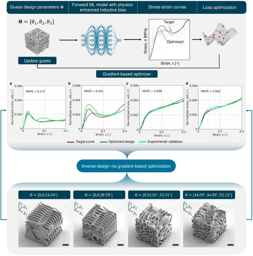
Figure 5: Deep learning-based inverse design framework Top: The forward ML model serves as a fast surrogate to evaluate the structure-property relations within an iterative gradient-based optimization scheme. The input to the optimization scheme is a target stress-strain curve (indicated in red) and the optimizer iteratively updates the guess design parameters until the loss between the predicted and target stress-strain curve is minimized. Middle: (a-d) We optimize for four target stress-strain curves which are not present in the training dataset. The stress-strain plots show the target (red), optimized (teal), and experimentally verified (green) stress-strain curves. Bottom: SEM images of the fabricated samples corresponding to the optimized design parameters and the green stress-strain curves in the middle panel. Scale bar, 20 µm.

We use the predictive capabilities of the forward ML model as a fast surrogate (to experiments) for inverse designing spinodal metamaterials with prescribed nonlinear stress-strain responses. Let $\mathcal{S}=\{(\hat{\varepsilon}_{t},\hat{\sigma}_{t})\ :\ t=1,\dots,T\}$ be a desired stress-strain response for quasi-static uniaxial compression loading discretized on $T>0$ points. We use the MAPE loss to formulate the inverse design task as an optimization:

$$\bm{\Theta},\hat{\bm{e}}_{i}\leftarrow\operatorname*{arg\,min}_{\bm{\Theta},\ i\in\{1,2,3\}}\ \frac{1}{T}\sum_{t=1}^{T}\left|\frac{\sigma^{(i)}(\hat{\varepsilon}_{t},\bm{\Theta})-\hat{\sigma}_{t}}{\hat{\sigma}_{t}}\right|.$$ (10)

The stress predictions $\sigma^{(i)}(\hat{\varepsilon}_{t},\bm{\Theta})$ are evaluated via the forward ML model using Eq. (5), where the superscript $(\cdot)^{(i)}$ indicates the model corresponding to the $\hat{\bm{e}}_{i}$ principal direction of loading (see Supplementary Information Section 4). This has two advantages: (i) the numerical optimization requires several evaluations of the stress predictions, which are orders of magnitude faster when performed via the forward ML model than experiments (or even simulations, if feasible); and (ii) while gradient-based optimization schemes (e.g., gradient descent[44]) are more efficient and stable than non-gradient-based methods, they require computing the sensitivities of the loss function with respect to the variables (in this case, $\bm{\Theta}$). Leveraging the computational graph and backpropagation of NNs[45], the forward ML model enables automatic differentiation[46] of the stress predictions $\sigma$ and in turn, the loss function with respect to $\bm{\Theta}$. In contrast to computationally intensive numerical differentiation (perturbing the input and re-evaluating the loss function), automatic differentiation provides analytically exact gradients and enables a more stable numerical optimization.

Here, we use the Adaptive Moment Estimation or Adam[47] optimizer to solve Eq. (10). We highlight that the inverse design challenge is ill-posed as multiple designs can exhibit the target stress-strain curve. To bypass this challenge, we perform the optimization for different initial guesses in parallel and select the design with the lowest MAPE loss at the end. Supplementary Information Section 4 provides additional details on the optimization protocols and a pseudocode is presented in Supplementary Information Algorithm 1.

To demonstrate the efficacy of our framework, we inversely design for target curves from our dataset, which were multiplied by a factor $\kappa$. This ensures that the target mechanical behavior is beyond the stress-strain curves which were provided in the limited experimentally generated training set. We present four distinct target curves and their respective optimization results in Figure 5a-d. For each target (red) we optimize the design parameters to obtain an optimized curve (teal). Finally, we fabricate and test the structures with the optimized design parameters (green). The first target (a) has a strain-softening region after the yield point, with a subsequent stress plateau. The second target (b) has a similar strain-softening region with a subsequent strain-hardening region. The third and fourth targets (c,d) exhibit a relatively stable, monotonically increasing stress-strain response. For the first target, the optimization framework proposes a lamellar structure ( $\bm{\Theta}=[0^{\circ},0^{\circ},24.34^{\circ}]$) oriented along the $\hat{\bm{e}}_{2}$-direction to achieve the desired stress-strain response. The fabricated structure matches the target response well with a MAPE of $17.4\%$. Most of the error stems from a strain-hardening region present in the fabricated sample, which the forward module was not able to predict. For the second target, also a lamellar structure ( $\bm{\Theta}=[0^{\circ},0^{\circ},38.78^{\circ}]$), the MAPE between the response of the fabricated sample and the target curve is $30\%$. Here, the three curves are dissonant, with the experiment showing a higher yield stress than what was predicted but a satisfactory match beyond $20\%$ strain. Although the curve was not matched well, the overall macro-structural behavior, i.e., strain-softening with subsequent strain-hardening, is captured with the optimized design parameters. For the third and fourth targets ($\bm{\Theta}=[0^{\circ},52.02^{\circ},52.31^{\circ}]$ and $\bm{\Theta}=[44.09^{\circ},46.83^{\circ},52.13^{\circ}]$), we observe an excellent match with the queried stress-strain behavior with MAPEs of 9.6% and 6.2%, respectively. The forward module had no problem in identifying the design parameters needed to match the queried out-of-dataset nonlinear response.

Validation on these four target curves demonstrates the validity of the proposed framework to capture highly nonlinear responses in complex 3D spinodal morphologies that lack internal symmetry and periodicity. While quantitative agreement between experimental and optimized responses improves for columnar or cubic morphologies, which have less pronounced anisotropy compared to lamellar ones, the overall qualitative response was always captured regardless of the $\bm{\Theta}$ representation. Specifically, in scenarios where micromechanical instabilities or failure events led to a macro-structural negative-stiffness responses, the framework accurately accounted for these features with closely matched stress and strain levels. Moreover, our results demonstrate that the physical basis chosen for our ML framework accurately describes the structural response of thick-shell spinodal structures at finite strains—a complex parameter space that is intractable to fully explore through high-fidelity simulations or experiments alone.

Conclusion

Designing complex spinodal metamaterials with a wide range of topologies and corresponding nonlinear mechanical behavior is challenging, especially when computational modeling is not feasible and experimental data is scarce. Here, we introduced a physics-enhanced ML and optimization framework that bypasses this challenge by directly using extremely sparse experimental data and enables the inverse design of spinodal structures with tailored finite-strain mechanical responses.

The lack of data for learning the structure-property relations is compensated by the physics-based inductive biases, which aid in identifying nonlinear responses such as instability- and localization-dominated responses. Tracing these responses back to nonconvex energetic potentials allows for a versatile framework that may be applied to variety of lightweight microstructures employed in the mechanical metamaterials community. Inspired from phase transformation modeling approaches, combining multiple convex (in strain) neural networks to form nonconvex but monotonically increasing potentials can accurately and efficiently capture complex nonlinear stress-strain behavior in presence of extreme and localized deformation including failure. At the same time, partial input convexity of PICNN architectures allows capturing arbitrary non-convex functional relations with the design parameters of spinodal metamaterials.

While we developed this framework for spinodal metamaterials, we note that the ML inverse design framework and the physics-enhanced inductive biases are general enough to be individually (or in combination) adapted for any class of metamaterials (e.g., truss, plate, or TPMS lattices) and data representation (e.g., vector, graph, or pixel/voxel-based parameterizations). The gradient-based optimization strategy can also be adapted to other approaches, including generative ML methods such as conditional variational autoencoders [48] and diffusion models [32]. Moreover, in this work, we have performed a comparatevely large number of high-fidelity experiments in both ex situ and in situ formats to assist in the understanding of the ML model from a physical basis. Compared to classical literature on experimental architected material explorations, which must balance a compromise of time-consuming fabrication and experimentation, we leverage microscale fabrication and testing to obtain an order-of-magnitude increase in data throughput—necessary for applicability to ML frameworks. From the 321 experiments performed in this work, we were able to capture the complex localized deformation behavior of thick-shelled spinodal morphologies, which led us to gain critical insights into the physical interpretation of our ML framework results. This work closes the gap in understanding the structure-to-property relations of high-relative-density spinodal morphologies at finite strains, relevant to applications of high energy absorption materials. The combination of using an experimentally generated dataset to train a physics-enhanced ML framework shows a promising avenue for designing and understanding the complex architected materials of the future.

Material and Methods

Sample fabrication

Before fabricating the final 107 spinodal morphologies, both a computational analysis and a manufacturing feasibility study were performed to find the appropriate fabrication parameters for this study (Supplementary Information Section 2.1 for details). From this study, a wave number of 5 was selected to generate the base shell unit cells. Then, a nominal shell thickness of 3 µm was chosen to ensure fabrication with minimal defects such as warping and to avoid self-intersection of shells upon fabrication. The generated spinodal shell meshes were thickened in Blender (3.3.1) using a solidify modifier.

After the final parameters were selected, the morphologies were fabricated using a two-photon lithography process with a Nanoscribe Photonic Professional GT2 (Nanoscribe GmbH) system, using IP-Dip photoresist and a 63$\times$ objective. A scan speed of 10,000 µm/s, laser power of 25 mW, slicing distance of 0.3 µm, and hatching distance of 0.2 µm were used.

Post-printing, the samples were developed in propyleneglycol-monomethyl-ether-acetate (PGMEA) for 40 to 60 minutes followed by immersion into isopropyl alcohol to remove any remaining PGMEA. Lastly, the samples underwent a critical point drying process (Tousimis Autosamdri-931). The fabricated unit cells had a relative density of approximately 40%, with average size of 92$\times$92$\times$92 µm³ and a shell thickness of 2.6 µm.

Nanomechanical experiments

We performed uniaxial quasi-static in situ and ex situ compression experiments using a 400-µm flat punch tip and a displacement-controlled nanoindenter (Alemnis AG). All experiments consisted of a compression to 50 µm. A strain rate of $10^{-3}$ s^-1 was maintained for all experiments. The in situ compressions were performed in a Zeiss SEM (Sigma HD VP) under the same testing conditions as the ex situ experiments. The stress-strain data was calculated by normalizing the load-data with the cross-sectional area and height of each sample.

To ensure IP-Dip photoresist properties stayed consistent between fabrication batches, monolithic IP-Dip pillars were fabricated and tested under the same conditions, providing measurement of Young’s modulus $E_{s}$ and yield strength (Supplementary Section 2.2). The modulus and yield strength for the IP-Dip photoresist were found to be $3.2\pm 0.3$ GPa and $77\pm 7$ MPa, respectively. We note that between all pillars tested, the standard deviation of both the modulus and yield strength were within 10%, showing consistency of properties between print batches (See Supplementary Information Figure 2).

ML Training details

Further implementation details regarding the Machine learning framework (Section 3), including the data preprocessing (Section 3.1), optimized hyperparameters (Table 2), implementation details of the PICNN (Section 3.3), training protocols (Section 3.4), and the gradient-based multi-initialization optimization scheme (Section 4) are provided in the Supplementary Information.

Declaration of competing interest

The authors declare that they have no known competing financial interests or personal relationships that could have appeared to influence the work reported in this paper.

Code availability

The codes developed in the current study will be freely open-sourced at the time of publication.

Data availability

The data generated in the current study will be made freely available at the time of publication.

References

- [1] Bückmann, T. et al. Tailored 3d mechanical metamaterials made by dip-in direct-laser-writing optical lithography. \JournalTitleAdvanced Materials 24, 2710–2714 (2012).
- [2] Meza, L. R., Das, S. & Greer, J. R. Strong, lightweight, and recoverable three-dimensional ceramic nanolattices. \JournalTitleScience 345, 1322–1326 (2014).
- [3] Meza, L. R. et al. Resilient 3d hierarchical architected metamaterials. \JournalTitleProceedings of the National Academy of Sciences 112, 11502–11507 (2015).
- [4] Vyatskikh, A. et al. Additive manufacturing of 3d nano-architected metals. \JournalTitleNature communications 9, 593 (2018).
- [5] Vangelatos, Z., Gu, G. X. & Grigoropoulos, C. P. Architected metamaterials with tailored 3d buckling mechanisms at the microscale. \JournalTitleExtreme Mechanics Letters 33, 100580 (2019).
- [6] Zheng, X. et al. Ultralight, ultrastiff mechanical metamaterials. \JournalTitleScience 344, 1373–1377 (2014).
- [7] Zhang, X. Y., Ren, X., Zhang, Y. & Xie, Y. M. A novel auxetic metamaterial with enhanced mechanical properties and tunable auxeticity. \JournalTitleThin-Walled Structures 174, 109162 (2022).
- [8] Wang, L. et al. Mechanical cloak via data-driven aperiodic metamaterial design. \JournalTitleProceedings of the National Academy of Sciences 119, e2122185119 (2022).
- [9] Kumar, S., Tan, S., Zheng, L. & Kochmann, D. M. Inverse-designed spinodoid metamaterials. \JournalTitlenpj Computational Materials 6, 73 (2020).
- [10] Zheng, L., Kumar, S. & Kochmann, D. M. Unifying the design space of truss metamaterials by generative modeling. \JournalTitlearXiv preprint arXiv:2306.14773 (2023).
- [11] Van’t Sant, S., Thakolkaran, P., Martínez, J. & Kumar, S. Inverse-designed growth-based cellular metamaterials. \JournalTitleMechanics of Materials 182, 104668 (2023).
- [12] Bastek, J.-H., Kumar, S., Telgen, B., Glaesener, R. N. & Kochmann, D. M. Inverting the structure–property map of truss metamaterials by deep learning. \JournalTitleProceedings of the National Academy of Sciences 119, e2111505119 (2022).
- [13] Bauer, J., Kraus, J. A., Crook, C., Rimoli, J. J. & Valdevit, L. Tensegrity metamaterials: toward failure-resistant engineering systems through delocalized deformation. \JournalTitleAdvanced Materials 33, 2005647 (2021).
- [14] Wu, W., Kim, S., Ramazani, A. & Cho, Y. T. Twin mechanical metamaterials inspired by nano-twin metals: Experimental investigations. \JournalTitleComposite Structures 291, 115580 (2022).
- [15] Saccone, M. A., Gallivan, R. A., Narita, K., Yee, D. W. & Greer, J. R. Additive manufacturing of micro-architected metals via hydrogel infusion. \JournalTitleNature 612, 685–690 (2022).
- [16] Tancogne-Dejean, T., Diamantopoulou, M., Gorji, M. B., Bonatti, C. & Mohr, D. 3d plate-lattices: an emerging class of low-density metamaterial exhibiting optimal isotropic stiffness. \JournalTitleAdvanced Materials 30, 1803334 (2018).
- [17] Al-Ketan, O. et al. Microarchitected stretching-dominated mechanical metamaterials with minimal surface topologies. \JournalTitleAdvanced Engineering Materials 20, 1800029 (2018).
- [18] Bonatti, C. & Mohr, D. Smooth-shell metamaterials of cubic symmetry: Anisotropic elasticity, yield strength and specific energy absorption. \JournalTitleActa Materialia 164, 301–321 (2019).
- [19] Portela, C. M. et al. Extreme mechanical resilience of self-assembled nanolabyrinthine materials. \JournalTitleProceedings of the National Academy of Sciences 117, 5686–5693 (2020).
- [20] Vidyasagar, A., Krödel, S. & Kochmann, D. M. Microstructural patterns with tunable mechanical anisotropy obtained by simulating anisotropic spinodal decomposition. \JournalTitleProceedings of the Royal Society A: Mathematical, Physical and Engineering Sciences 474, 20180535 (2018).
- [21] Hsieh, M.-T., Endo, B., Zhang, Y., Bauer, J. & Valdevit, L. The mechanical response of cellular materials with spinodal topologies. \JournalTitleJournal of the Mechanics and Physics of Solids 125, 401–419 (2019).
- [22] Guo, Y., Sharma, S. & Kumar, S. Inverse designing surface curvatures by deep learning. \JournalTitlearXiv preprint arXiv:2309.00163 (2023).
- [23] Bauer, J., Sala-Casanovas, M., Amiri, M. & Valdevit, L. Nanoarchitected metal/ceramic interpenetrating phase composites. \JournalTitleScience Advances 8, eabo3080 (2022).
- [24] Zheng, L., Kumar, S. & Kochmann, D. M. Data-driven topology optimization of spinodoid metamaterials with seamlessly tunable anisotropy. \JournalTitleComputer Methods in Applied Mechanics and Engineering 383, 113894 (2021).
- [25] Senhora, F. V., Sanders, E. D. & Paulino, G. H. Optimally-Tailored Spinodal Architected Materials for Multiscale Design and Manufacturing. \JournalTitleAdvanced Materials 34, 2109304, DOI: 10.1002/adma.202109304 (2022).
- [26] Zhang, Y., Hsieh, M.-T. & Valdevit, L. Mechanical performance of 3d printed interpenetrating phase composites with spinodal topologies. \JournalTitleComposite Structures 263, 113693 (2021).
- [27] Guell Izard, A., Bauer, J., Crook, C., Turlo, V. & Valdevit, L. Ultrahigh energy absorption multifunctional spinodal nanoarchitectures. \JournalTitleSmall 15, 1903834 (2019).
- [28] Hsieh, M.-T., Begley, M. R. & Valdevit, L. Architected implant designs for long bones: Advantages of minimal surface-based topologies. \JournalTitleMaterials & Design 207, 109838 (2021).
- [29] Wojciechowski, B., Xue, Y., Rabbani, A., Bolton, J. S. & Sharma, B. Additively manufactured spinodoid sound absorbers. \JournalTitleAdditive Manufacturing 71, 103608 (2023).
- [30] Röding, M., Wåhlstrand Skärström, V. & Lorén, N. Inverse design of anisotropic spinodoid materials with prescribed diffusivity. \JournalTitleScientific Reports 12, 17413 (2022).
- [31] Soyarslan, C., Bargmann, S., Pradas, M. & Weissmüller, J. 3d stochastic bicontinuous microstructures: Generation, topology and elasticity. \JournalTitleActa materialia 149, 326–340 (2018).
- [32] Bastek, J.-H. & Kochmann, D. M. Inverse-design of nonlinear mechanical metamaterials via video denoising diffusion models. \JournalTitlearXiv preprint arXiv:2305.19836 (2023).
- [33] Ha, C. S. et al. Rapid inverse design of metamaterials based on prescribed mechanical behavior through machine learning. \JournalTitleNature Communications 14, 5765 (2023).
- [34] Lee, S., Zhang, Z. & Gu, G. X. Deep learning accelerated design of mechanically efficient architected materials. \JournalTitleACS Applied Materials & Interfaces 15, 22543–22552 (2023).
- [35] Lee, D., Chen, W., Wang, L., Chan, Y.-C. & Chen, W. Data-driven design for metamaterials and multiscale systems: A review. \JournalTitleAdvanced Materials 2305254 (2023).
- [36] Wilt, J. K., Yang, C. & Gu, G. X. Accelerating auxetic metamaterial design with deep learning. \JournalTitleAdvanced Engineering Materials 22, DOI: 10.1002/adem.201901266 (2020).
- [37] Mao, Y., He, Q. & Zhao, X. Designing complex architectured materials with generative adversarial networks. \JournalTitleScience Advances 6, DOI: 10.1126/sciadv.aaz4169 (2020).
- [38] Meyer, P. P., Bonatti, C., Tancogne-Dejean, T. & Mohr, D. Graph-based metamaterials: Deep learning of structure-property relations. \JournalTitleMaterials & Design 223, 111175, DOI: 10.1016/j.matdes.2022.111175 (2022).
- [39] Cahn, J. W. On spinodal decomposition. \JournalTitleActa metallurgica 9, 795–801 (1961).
- [40] Iyer, A. et al. Designing anisotropic microstructures with spectral density function. \JournalTitleComputational Materials Science 179, 109559, DOI: 10.1016/j.commatsci.2020.109559 (2020).
- [41] Kumar, S., Vidyasagar, A. & Kochmann, D. M. An assessment of numerical techniques to find energy-minimizing microstructures associated with nonconvex potentials. \JournalTitleInternational Journal for Numerical Methods in Engineering 121, 1595–1628 (2020).
- [42] As’ ad, F., Avery, P. & Farhat, C. A mechanics-informed artificial neural network approach in data-driven constitutive modeling. \JournalTitleInternational Journal for Numerical Methods in Engineering 123, 2738–2759 (2022).
- [43] Amos, B., Xu, L. & Kolter, J. Z. Input convex neural networks. In International Conference on Machine Learning, 146–155 (PMLR, 2017).
- [44] Hardt, M., Recht, B. & Singer, Y. Train faster, generalize better: Stability of stochastic gradient descent. In International conference on machine learning, 1225–1234 (PMLR, 2016).
- [45] LeCun, Y., Bengio, Y. & Hinton, G. Deep learning. \JournalTitleNature 521, 436–444, DOI: 10.1038/nature14539 (2015).
- [46] Paszke, A. et al. Pytorch: An imperative style, high-performance deep learning library. In Wallach, H. et al. (eds.) Advances in Neural Information Processing Systems, vol. 32 (Curran Associates, Inc., 2019).
- [47] Kingma, D. P. & Ba, J. Adam: A method for stochastic optimization. \JournalTitlearXiv preprint arXiv:1412.6980 (2014).
- [48] Glaesener, R. et al. Predicting the influence of geometric imperfections on the mechanical response of 2d and 3d periodic trusses. \JournalTitleActa Materialia 254, 118918, DOI: 10.1016/j.actamat.2023.118918 (2023).