Low-energy perspective on two-orbital Hund metals and the case of LaNiO₂

Abstract

The Hund-metal route to strong correlations continues to attract large interest in the condensed-matter community. The question arose to what extent it applies to the infinite-layer nickelates and, as a related question, to two-orbital systems in general. Here, we provide a low-energy perspective on this topic through a dynamical mean-field study using the numerical renormalization group (NRG) as a real-frequency impurity solver. We find that the RG flow from high to low energy is a uniquely adequate tool to reveal two-stage Kondo screening (2SKS), a fascinating mechanism for Hund physics. Further, we show that 2SKS takes place in a quarter-filled two-orbital system, but can be easily suppressed by a sufficiently large crystal-field splitting. We apply these insights to LaNiO₂ using a recently proposed two-orbital model and show that it is indeed the crystal-field splitting that suppresses multiorbital phenomena in this scenario. Our general findings open the way for further explorations of 2SKS, and we propose a way of reviving low-energy Hund physics in LaNiO₂ by counteracting the crystal field.

I introduction

Recently, the physics of Hund metals Yin et al. (2011), where not only Hubbard $U$ but also Hund’s coupling $J$ plays a key role for the electronic correlations, is discussed in a broader context than originally anticipated. Archetypal Hund metals (see Ref. Georges et al. (2013) for a review) are iron pnictides and chalcogenides as well as ruthenates, whose occupancy of the $d$ shell is away from half-filling or single occupancy. However, it was also proposed that Hund physics is relevant for the half-filled NiS_2-xSe_x Jang et al. (2021); Park et al. or for the infinite-layer nickelates (which bear similarities to the cuprates).

Indeed, the finding of unconventional superconductivity in the nickelates Li et al. (2019) has revived the theoretical interest in these compounds. There are by now many works using the combination of density functional theory and dynamical mean-field theory (DFT+DMFT) Georges et al. (1996); Kotliar et al. (2006) on 112 nickelates (such as NdNiO₂ and LaNiO₂) Karp et al. (2020a); Lechermann (2020a); Gu et al. (2020); Ryee et al. (2020); Si et al. (2020); Kitatani et al. (2020); Lechermann (2020b); Leonov et al. (2020); Wang et al. (2020a); Kang and Kotliar (2021); Kang et al. (2023). Some of them emphasize more the single-orbital nature of correlations with an additional self-doping band Karp et al. (2020a); Kitatani et al. (2020), others evoke a multiorbital Hund-metal picture Wang et al. (2020a); Kang et al. (2023). Recently Kang and Kotliar (2021), it was pointed out that, while the $d_{x^{2}-y^{2}}$ orbital dominates the low-energy properties, there can be important orbital fluctuations at intermediate energies.

Understanding the influence of Hund physics in 112 nickelates, especially within their Ni $e_{g}$ orbitals, requires answering a simpler and more general question: To what extent can Hund physics be present in two-orbital systems, where nonzero integer occupancy is bound to either half-filling or single occupancy (of an electron or a hole)? Addressing this question, Ref. Ryee et al. (2021) studied a quarter-filled two-orbital model, finding that one can indeed distinguish a weak Hund metal. This study employed a Quantum Monte Carlo imaginary-frequency DMFT impurity solver Gull et al. (2011); Choi et al. (2019). Here, we confirm this finding and provide an additional perspective by using the numerical renormalization group (NRG) Bulla et al. (2008) as a real-frequency impurity solver, which offers exponentially fine low-energy resolution and a physically transparent RG flow.

The goal of this paper is twofold. First, we take a minimal-model point of view and analyze Hund-metal characteristics in an orbital-symmetric two-orbital system with occupancy 1, as compared to three-orbital systems with occupancy 1 or 2. Through properties not studied in Ref. Ryee et al. (2021) (real-frequency spectra and RG flows), we substantiate their finding of a weak Hund metal. We then scrutinize the influence of a crystal-field splitting between the two orbitals, capable of suppressing multiorbital phenomena. Second, we turn to a material-realistic setting and analyze a two-orbital description of LaNiO₂ Sakakibara et al. (2020); Hepting et al. (2020); Adhikary et al. (2020); Wan et al. (2021); Kang and Kotliar (2021) at quarter-filling. We show that—in this specific scenario—multiorbital Hund physics is suppressed by a large crystal-field splitting of $|\Delta|\!\approx\!0.8\,\mathrm{eV}$. This is evidenced by comparing low-energy properties of the $d_{x^{2}-y^{2}}$ orbital obtained from a two- and a one-orbital calculation and by demonstrating the resurgence of Hund physics at vanishing $|\Delta|$. The models and the method are briefly introduced in Sec. II. The general model analysis is contained in Secs. III.1–III.4 and the LaNiO₂ study in Sec. III.5. We conclude in Sec. IV. Appendix A contains additional numerical results and App. B general statements about interaction Hamiltonians.

II Models and method

We consider multiorbital Hubbard models of the type

$$\textstyle H=\sum_{ijmm^{\prime}\sigma}d^{\dagger}_{im\sigma}h^{mm^{\prime}}_{ij}d_{jm^{\prime}\sigma}+\sum_{i}H_{\mathrm{int}}[d_{im\sigma}],$$ (1)

where $d^{\dagger}_{im\sigma}$ creates an electron at site $i$, in orbital $m\!\in\!\{1,\kern-1.49994pt.\kern-0.50003pt.\kern-0.50003pt.,\!M\}$, and with spin $\sigma\!\in\!\{\uparrow,\downarrow\}$. For the first part of our results, the hopping matrix is taken to be diagonal in orbital space and such that it corresponds to a semicircular density of states of half bandwidth $D\!=\!1$ (Bethe lattice). We consider both the orbital-symmetric case with on-site energies $\epsilon_{m}\!=\!\epsilon_{m^{\prime}}$ for two and three orbitals as well as two-orbital systems with a crystal-field splitting $\Delta\!=\!\epsilon_{1}\!-\!\epsilon_{2}$. The three-orbital case with occupancy 2 serves as our reference system for “canonical” Hund physics Georges et al. (2013); Stadler et al. (2015); Ryee et al. (2023). In the second part of our results, the hopping matrix is taken from a two-orbital model fitted to the band structure of LaNiO₂. It thus has off-diagonal elements in orbital space, except for the local part $i\!=\!j$. We remark that three-orbital models of LaNiO₂ were suggested too Nomura et al. (2019); Liu et al. (2020); Karp et al. (2020a), but these are not considered in the present work.

The local interaction is chosen as ($n_{m\sigma}=d^{\dagger}_{m\sigma}d_{m\sigma}$)

$$H_{\mathrm{int}} =U\sum_{m}n_{m\uparrow}n_{m\downarrow}+\!\sum_{m<m^{\prime},\sigma\sigma^{\prime}}\!(U^{\prime}-\delta_{\sigma\sigma^{\prime}}J)n_{m\sigma}n_{m^{\prime}\sigma^{\prime}}$$

$$\ -J\sum_{m\neq m^{\prime}}d^{\dagger}_{m\uparrow}d_{m\downarrow}d^{\dagger}_{m^{\prime}\downarrow}d_{m^{\prime}\uparrow}.$$ (2)

We show in App. B that, at $U^{\prime}\!=\!U\!-\!J$, this realizes the Dworin–Narath (DN) Hamiltonian $(U-\tfrac{3}{2}J)\tfrac{1}{2}N(N\!-\!1)-J{\bm{S}}^{2}+\tfrac{3}{4}JN$. At $U^{\prime}\!=\!U\!-\!2J$, it corresponds to the Hubbard–Kanamori (HK) Hamiltonian $(U-3J)\tfrac{1}{2}N(N\!-\!1)-2J{\bm{S}}^{2}-\tfrac{1}{2}J{\bm{L}}^{2}+\tfrac{2+M}{2}JN$ (${\bm{L}}\!\equiv\!L_{3}$ for $M\!=\!2$), except that pair-hopping is neglected. The latter restriction does not qualitatively change the low-energy Hund physics but simplifies the numerics considerably Kugler et al. (2020). When ambiguous, we attach a subscript to the Hund’s coupling, $J_{\mathrm{DN}}$ or $J_{\mathrm{HK}}$, to specify which Hamiltonian is being used.

We follow Ref. Ryee et al. (2021) in defining an average (opposite-spin) Hubbard interaction $\bar{U}\!=\!\frac{1}{M^{2}}\sum_{mm^{\prime}}U_{mm^{\prime}}$ (called $U_{\mathrm{av}}$ in Ref. Ryee et al. (2021)), where $U_{mm}\!=\!U$ and $U_{m\neq m^{\prime}}\!=\!U^{\prime}$. This yields

$$\bar{U}=U^{\prime}\!+\!\frac{U-U^{\prime}}{M}=\begin{cases}U\!-\!\frac{M-1}{M}J_{\mathrm{DN}},\!\!&U^{\prime}=U\!-\!J_{\mathrm{DN}}\\ U\!-\!2\frac{M-1}{M}J_{\mathrm{HK}},\!\!&U^{\prime}=U\!-\!2J_{\mathrm{HK}}\end{cases}.$$ (3)

The cases relevant for us are listed in Table 1, along with the corresponding values of the atomic gap $\Delta_{\mathrm{at}}\!=\!U^{\prime}\!-\!J$ Georges et al. (2013).

	$M\!=\!2$ DN	$M\!=\!2$ HK	$M\!=\!3$ DN	$M\!=\!3$ HK
$\bar{U}$	$U\!-\!\tfrac{1}{2}J$	$U\!-\!J$	$U\!-\!\tfrac{2}{3}J$	$U\!-\!\tfrac{4}{3}J$
$\Delta_{\mathrm{at}}\!=\!U^{\prime}\!-\!J$	$U\!-\!2J$	$U\!-\!3J$	$U\!-\!2J$	$U\!-\!3J$

Table 1: Average (opposite-spin) Hubbard interaction $\bar{U}$ and atomic gap $\Delta_{\mathrm{at}}$ for $M\!=\!2$ or $3$ orbitals using the DN or HK Hamiltonian.

$M$	$H_{\mathrm{int}}$	Symmetry	$N_{\mathrm{kp}}$	$N_{\mathrm{kp}}^{*}$
3	DN	$\textrm{U}(1)_{\textrm{ch}}\otimes\textrm{SU}(2)_{\textrm{sp}}\otimes\textrm{SU}(3)_{\textrm{orb}}$	$20\textsf{k}$	$800\textsf{k}$
2	DN	$\textrm{U}(1)_{\textrm{ch}}\otimes\textrm{SU}(2)_{\textrm{sp}}\otimes\textrm{SU}(2)_{\textrm{orb}}$	$15\textsf{k}$	$130\textsf{k}$
3	HK	$\bigotimes_{m=1}^{3}\textrm{U}(1)_{\textrm{ch},m}\otimes\textrm{SU}(2)_{\textrm{sp}}$	$100\textsf{k}$	$350\textsf{k}$
2	HK	$\bigotimes_{m=1}^{2}\textrm{U}(1)_{\textrm{ch},m}\otimes\textrm{SU}(2)_{\textrm{sp}}$	$30\textsf{k}$	$90\textsf{k}$

Table 2: Symmetries used and multiples $N_{\mathrm{kp}}$ (or states $N_{\mathrm{kp}}^{*}$) maximally kept during the NRG iterative diagonalization ($1\textsf{k}$ denotes $10^{3}$).

We treat our models within the DMFT approximation Georges et al. (1996); Kotliar et al. (2006), where the lattice Hamiltonian is mapped onto a self-consistently determined impurity model. The latter is then solved with NRG Bulla et al. (2008) at zero temperature ($T\!=\!10^{-6}$ or $10^{-8}$ in practice) assuming paramagnetism. We employ the full density-matrix NRG Peters et al. (2006); Weichselbaum and von Delft (2007) in a state-of-the-art implementation based on the QSpace tensor library Weichselbaum (2012a); *Weichselbaum2012b; *Weichselbaum2020. We use an adaptive broadening scheme Lee and Weichselbaum (2016); Lee et al. (2017) and a symmetric improved estimator for the self-energy Kugler (2022). In the cases without $\textrm{SU}(M)$ orbital symmetry, we interleave the Wilson chains for increased efficiency Mitchell et al. (2014); Stadler et al. (2016). For the overview of quasiparticle weights, we used $n_{z}\!=\!2$ shifted discretization grids Žitko and Pruschke (2009); for all other calculations, $n_{z}\!=\!4$. We purposefully pick the same NRG discretization parameter $\Lambda\!=\!4$ for all calculations, in order to have the most straightforward comparison between different flow diagrams. All available charge, spin, and orbital symmetries are exploited, as summarized in Table 2. There, we also give the maximal number of multiplets $N_{\mathrm{kp}}$ (and corresponding number states $N_{\mathrm{kp}}^{*}$) kept during the iterative diagonalization.

The quantities of interest are the (retarded) local self-energies $\Sigma_{m}(\omega)$ and associated quasiparticle weights $Z_{m}\!=\![1\!-\!\partial_{\omega}\mathrm{Re}\!\;\Sigma_{m}(\omega)|_{\omega=0}]^{-1}$, the local spectral functions $\mathcal{A}_{m}(\omega)$ and associated occupancy per orbital $n_{m}\!=\!\int\mathrm{d}\omega f_{\omega}\mathcal{A}_{\mathrm{loc},m}(\omega)$ (where $f_{\omega}\!=\![1+\exp(\omega/T)]^{-1}$), and the (retarded) local susceptibilities $\chi\!=\!\chi^{\prime}\!-\!\mathrm{i}\pi\chi^{\prime\prime}$ defined via the spin and orbital operators (cf. App. B). We further analyze NRG flow diagrams Bulla et al. (2008) (see Ref. Kugler et al. (2020) for how $E_{\ell}$ is mapped to $\omega$). Note that, for the models solved with interleaved NRG, we perform an additional diagonalization without interleaving in order to have flow diagrams comparable to those from the other models. Finally, in our LaNiO₂ study, we also consider the momentum-resolved spectral function $\mathcal{A}({\bm{k}},\omega)\!=\!-\frac{1}{\pi}\mathrm{Im}\!\;\mathrm{Tr}[\omega\!+\!\mu\!-\!{\bm{h}}({\bm{k}})\!-\!{\bm{\Sigma}}(\omega)]^{-1}$, following from the matrix-valued hopping and self-energy.

III Results

III.1 General considerations

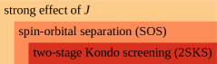
Figure 1: Venn diagram showing various effects of Hund’s coupling $J$. The arguably most intricate effect is two-stage Kondo screening (2SKS): upon decreasing energy, first, orbital fluctuations are dynamically (Kondo-) screened, then spin fluctuations. This phenomenon was dubbed spin-orbital separation (SOS) Stadler et al. (2015), with $T^{\mathrm{K}}_{\mathrm{sp}}\!\ll\!T^{\mathrm{K}}_{\mathrm{orb}}\!\ll\!U,J$. However, SOS can also occur more trivially. In a half filled system at finite $J$, e.g., orbital fluctuations are suppressed at energies below $J$ (or, in systems with a crystal field $\Delta$, at energies below $\Delta$ Kugler et al. (2019)). If, in abuse of notation, one still calls this energy scale $\textrm{``}T^{\mathrm{K}}_{\mathrm{orb}}\textrm{''}$, one then has $T^{\mathrm{K}}_{\mathrm{sp}}\!\ll\!\textrm{``}T^{\mathrm{K}}_{\mathrm{orb}}\textrm{''}\!\sim\!J,\Delta$. Finally, $J$ not only affects low-energy Kondo physics but also (“high-energy”) atomic physics, like orbital occupancies. Thereby, it, e.g., facilitates an orbital-selective Mott phase in systems with broken orbital symmetry de’ Medici (2011) (see also Ref. Kugler and Kotliar (2022)).

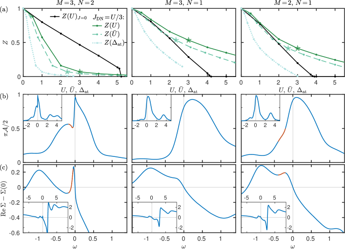
Figure 2: (a) Quasiparticle weight $Z$ as a function of $U$, $\bar{U}$, or $\Delta_{\mathrm{at}}$. The Janus effect ($Z|_{J\neq 0}\!<\!Z|_{J=0}$ for small $U$, $Z|_{J\neq 0}\!>\!Z|_{J=0}$ for large $U$) is strikingly clear for $(M,N)\!=\!(3,2)$ and somewhat discernible for $(M,N)\!=\!(2,1)$ when going from $Z(U)$ to $Z(\bar{U})$. (b) Spectral functions. The red line indicates the orbital-resonance shoulder. (c) Real part of self-energies. The red line indicates the corresponding inverted slope.

Hund’s coupling $J$ can affect interacting systems in various ways. For instance, $J$ changes the energies of atomic configurations and thereby influences their relative probabilities. In both the DN and the HK Hamiltonians, $J$ acts more strongly (with a larger prefactor) on the spin than on the orbital operators squared. Thereby, it naturally induces an asymmetry between the spin and orbital sectors. In the study of Kondo scales $T^{\mathrm{K}}$, indicating below which energies spin and orbital fluctuations are dynamically screened, this asymmetry with $T^{\mathrm{K}}_{\mathrm{sp}}\!\ll\!T^{\mathrm{K}}_{\mathrm{orb}}$ was dubbed spin-orbital separation (SOS) Stadler et al. (2015, 2019). Besides the Kondo screening mechanism, fluctuations can also be quenched more trivially, say, by atomic energy considerations. In a half-filled system at finite $J$, e.g., the atomic ground state is an orbital singlet, and orbital fluctuations are suppressed at energies below the bare parameter $J$. Similarly, in systems with large crystal-field splitting $\Delta$, orbital fluctuations are suppressed at energies below the bare parameter $\Delta$. The various aspects of $J$ mentioned above are illustrated in Fig. 1. In the following, we focus on one particular aspect: the highly nontrivial form of SOS induced by two-stage Kondo screening (2SKS).

How does the effect of $J$, and 2SKS in particular, depend on the number of orbitals $M$ and the occupancy $N$? From an atomic perspective, $J$ splits the manifold of energy eigenstates with two or more electrons, giving preference to the high-spin state. Accordingly, this directly affects the atomic ground state for $N\!\geq\!2$, while it only affects excited states for $N\!=\!1$. Going beyond the atomic picture, early works Yin et al. (2012); Aron and Kotliar (2015) utilized a multiorbital Schrieffer–Wolff transformation. The spin Kondo coupling in a one-orbital system is $J^{\mathrm{K}}_{\mathrm{sp}}\!=\!2V^{2}(\frac{1}{\Delta E_{-}}\!+\!\frac{1}{\Delta E_{+}})$ where $\Delta E_{\pm}\!>\!0$ is the energy difference to the states with charge $\pm 1$ w.r.t. the ground state. In the one-orbital example, these are $\Delta E_{+}\!=\!\epsilon\!+\!U$ and $\Delta E_{+}\!=\!-\epsilon$, whence the well-known result $J^{\mathrm{K}}_{\mathrm{sp}}\!=\!2V^{2}\frac{U}{(\epsilon+U)(-\epsilon)}$ and $J^{\mathrm{K}}_{\mathrm{sp}}\!=\!8V^{2}/U$ at the particle-hole symmetric point $\epsilon\!=\!-U/2$ follows. In multiorbital systems (w.l.o.g. $M\!>\!N$), it was found Yin et al. (2012); Aron and Kotliar (2015) that $J^{\mathrm{K}}_{\mathrm{sp}}\!=\!\frac{2}{M}V^{2}(\frac{1}{\Delta E_{-}}-\frac{M-N}{N+1}\frac{1}{\Delta E_{+}})$. By the negative sign, $J^{\mathrm{K}}_{\mathrm{sp}}$ is reduced, thereby suppressing the spin Kondo temperature. (Note that an integer occupancy is achieved by balancing charge fluctuations to the adjacent sectors, so often times $\Delta E_{-}\!\approx\!\Delta E_{+}$.) Importantly, however, this statement applies to all values of $M$ and $N\!<\!M$. Hence, in contrast to the atomic perspective, it does not give preference to Hund physics in, say, systems with $(M,N)\!=\!(3,2)$ over those with $(M,N)\!=\!(2,1)$.

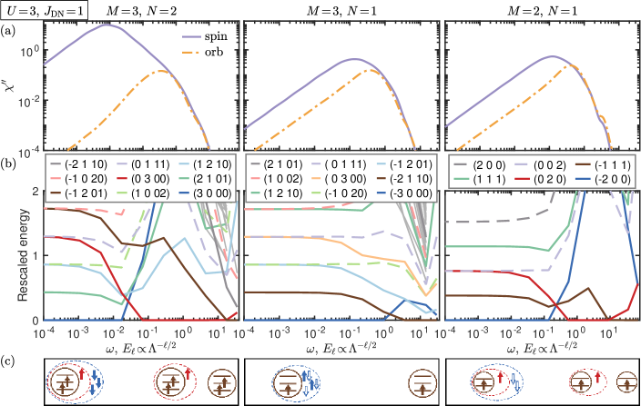
Figure 3: (a) Susceptibilities showing SOS: $\chi^{\prime\prime}_{\mathrm{sp}}$ is peaked at higher frequencies than $\chi^{\prime\prime}_{\mathrm{orb}}$. (b) NRG flow diagrams. The legend gives the charge (w.r.t. half-filling), spin, and orbital quantum numbers. (c) Pictorial representation of the ground states during the flow. The systems at charge one away from half-filling can realize an intermediate orbital-singlet spin-triplet state (red) at the lowest energy and thus experience 2SKS.

III.2 Single-particle properties in orbital-symmetric models

Let us now turn to numerical results. For the orbital-symmetric models, we employ the DN Hamiltonian, but the same behavior is observed for the HK Hamiltonian, see App. A. Figure 2(a) shows how $Z$ depends on the interaction strength in various settings and three filling cases: $(M,N)\!\in\!\{(3,2),(3,1),(2,1)\}$. First, increasing $U$ at $J\!=\!0$ (black lines), one finds a Mott insulator for sufficiently large $U$ in all three cases. Finite $J$ changes the behavior drastically, see the (dark) green line for $Z(U)$ at $J\!=\!U/3$.

The left panel $(M,N)\!=\!(3,2)$ displays the familiar Janus effect de’ Medici et al. (2011); Georges et al. (2013): compared to the black curve, $Z$ at finite $J$ drops down for small $U$ and then flattens again for larger $U$, so that $Z(U)|_{J\neq 0}$ exceeds $Z(U)|_{J=0}$ for $U\!\gtrsim\!5$. The latter property is a rather trivial atomic effect, as $J$ reduces the atomic gap $\Delta_{\mathrm{at}}\!=\!U^{\prime}\!-\!J$ away from half-filling de’ Medici et al. (2011); Georges et al. (2013). Indeed, this effect disappears if replacing $U$ by $\Delta_{\mathrm{at}}$ as the independent variable, and one has $Z(\Delta_{\mathrm{at}})|_{J\neq 0}\!<\!Z(U\!=\!\bar{U}\!=\!\Delta_{\mathrm{at}})|_{J=0}$ throughout. By contrast, the sharp drop of $Z$ at relatively small $U$ is a manifestation of Hund physics, i.e., strong correlations induced by Hund-$J$ at moderate Hubbard-$U$. As explained in Ref. de’ Medici et al. (2011), this is attributed to lifting the degeneracy of the atomic ground state (from 15-fold to 9-fold degenerate Georges et al. (2013)).

In the middle panel, $(M,N)\!=\!(3,1)$, there is no such Janus effect. Instead, finite $J$ increases $Z(U)$ for all $U$ (an effect that is again eliminated by switching from $Z(U)$ to $Z(\Delta_{\mathrm{at}})$). The right panel, $(M,N)\!=\!(2,1)$, also has $Z(U)|_{J\neq 0}\!>\!Z(U)|_{J=0}$. Perhaps, one might say that the initial decrease and subsequent flattening of $Z(U)_{J\neq 0}$ is slightly more pronounced in the $(M,N)\!=\!(2,1)$ than in the $(M,N)\!=\!(3,1)$ case.

In Ref. Ryee et al. (2021), it was argued that $\bar{U}$ instead of $U$ provides a better reference on the horizontal axis. Going from $Z(U)$ to $Z(\bar{U})$ shifts the $Z|_{J\neq 0}$ curve to the left by a relatively small amount (compared to going from $Z(U)$ to $Z(\Delta_{\mathrm{at}})$) proportional to $J$ (and thus $U$), see the dashed line in Fig. 2(a) and Table 1. The qualitative behavior in the left and middle panels of Fig. 2(a) remains basically unchanged. For the right panel, one might now argue that $Z(\bar{U})|_{J\neq 0}$ initially drops to an appreciable extent below $Z(U\!=\!\bar{U})|_{J=0}$ and then crosses through $Z(U\!=\!\bar{U})|_{J=0}$ due to a moderate flattening. In this way, one may say that $J$ slightly increases the correlation strength at $\bar{U}\!\sim\!1$, and, thus, the system for $(M,N)\!=\!(2,1)$ constitutes a weak Hund metal Ryee et al. (2021). However, since the splitting of atomic energy manifolds by $J$ affects only the excited states for $(M,N)\!=\!(2,1)$ (and not the ground state, as for $(M,N)\!=\!(3,2)$), the drop in $Z$ is much smaller for $(M,N)\!=\!(2,1)$ than for $(M,N)\!=\!(3,2)$.

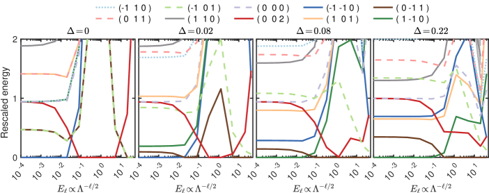
Figure 4: NRG flow diagrams at variable crystal-field splitting $\Delta$. The intermediate spin-triplet ground state (present in regions where the red line reaches zero) is only found for $|\Delta|\!\lesssim\!T^{\mathrm{K}}_{\mathrm{orb}}(\Delta\!=\!0)/2$.

Next, Figs. 2(b) and 2(c) show the spectral function and the real part of the self-energy in each case at $U\!=\!3$ and $J\!=\!1$ (the point indicated by a star in Fig. 2(a)). The insets in Fig. 2(b) display $\mathcal{A}$ on a wide-energy window, while the main plots focus on the quasiparticle peak. An intriguing feature observed in Hund metals is a orbital-resonance shoulder Stadler et al. (2015, 2019); Kugler et al. (2019) in the left part (for $N\!<\!M$) of the quasiparticle peak. Indeed, such a shoulder (marked in red) is very pronounced for $(M,N)\!=\!(3,2)$ and somewhat visible for $(M,N)\!=\!(2,1)$. In $\mathrm{Re}\!\;\Sigma$, this corresponds to an inverted slope or retracted renormalization (marked in red) Iwasawa et al. (2005); Mravlje et al. (2011); Stricker et al. (2014); Wadati et al. (2014); Kugler et al. (2019, 2020); Karp et al. (2020b). The inverted slope is also strikingly clear for $(M,N)\!=\!(3,2)$ and only somewhat discernible for $(M,N)\!=\!(2,1)$. Nevertheless, the fact that both features occur for $(M,N)\!=\!(3,2)$ and (albeit less pronounced) for $(M,N)\!=\!(2,1)$ corroborates the notion of a weak Hund metal in the latter case. Note that they are also found in rather different settings. For instance, as elaborated in Ref. Kugler et al. (2019), they persist when introducing a crystal-field splitting $\Delta$. Upon increasing $\Delta$ and approaching an orbital-selective Mott phase, they eventually change in nature from an orbital resonance (corresponding to 2SKS) to a separate doublon-holon peak (atomic-like). The same behavior occurs for the two-orbital setting with crystal-field splitting analyzed below.

III.3 NRG flow in orbital-symmetric models

We now inspect SOS and 2SKS via the susceptibilities and the NRG flow diagrams in each case. From $\chi^{\prime\prime}_{\mathrm{sp}}$ and $\chi^{\prime\prime}_{\mathrm{orb}}$ in Fig. 3(a), one readily observes SOS Stadler et al. (2016, 2019): the peak of the orbital susceptibility (indicating that orbital fluctuations get screened) occurs at a higher energy than the peak of the spin susceptibility (indicating that spin fluctuations get screened). This phenomenon is very pronounced for $(M,N)\!=\!(3,2)$ and weakly present in the other two cases. Whether 2SKS causes SOS is revealed by the NRG flow.

In Figs. 3(b) and 3(c), we present the NRG flow diagrams (to be read from right to left) and a pictorial representation of the ground state in different parts of the RG flow, following Refs. Stadler et al. (2019); Walter et al. (2020). The legend in Fig. 3(b) gives the U(1) charge (relative to half-filling), SU(2) spin (twice $S^{z}$) and SU($M$) orbital quantum numbers. At the beginning of the flow (i.e., at high energy, to the right in each panel of Fig. 3(b)), the system is fully described by an atomic picture. There, the ground state (brown line) can be represented by $N$ (aligned) spins symmetrically placed in $M$ orbitals. Going to lower energies (leftward in the plots), the effect of the environment (the self-consistently determined bath) comes into play.

The left panel, $(M,N)\!=\!(3,2)$, is our reference system for Hund physics and 2SKS. One clearly observes an extended region of the flow where the lowest-energy state (red line) involves the impurity with an additional bath electron (charge increased by one) that screens the orbital moment (quantum number $00$) and further increases the spin (quantum number $3$). This is part 1 of 2SKS. At the end of the flow (at low energy, to the left of the plot), three more bath electrons subsequently screen the magnetic moment (blue line; charge increased by 3, zero spin and orbital quantum numbers) Stadler et al. (2019); Walter et al. (2020). This is part 2 of 2SKS, yielding the Fermi liquid.

For $(M,N)\!=\!(3,1)$, such a 2SKS is not observed. As the system is further away from half-filling, an intermediate orbital-singlet and spin-tripled state would require the impurity to temporarily bind two bath electrons. Instead, the system directly flows from the atomic state (brown line, one electron in three orbitals) to a fully screened ground state (blue line).

Now, for $(M,N)\!=\!(2,1)$, again one away from half-filling, we do 2SKS: First, the orbital moment of one electron in two orbitals (brown line) is screened by one bath electron. The resulting spin triplet (red line) is then screened by two bath holes, leading to the fully screened Fermi-liquid ground state (blue line). Whether the final screening is achieved by electrons or holes depends on the detailed shape of the particle-hole asymmetric hybridization function at low energies. As before, Hund-metal signatures (here 2SKS) are observed for three and two orbitals at charge one away from half-filling, but much weaker so for $M\!=\!2$ than for $M\!=\!3$.

We end this section with a note of caution. The RG flow in NRG is discrete, owing to the logarithmic discretzation with $\Lambda\!>\!1$. Even–odd oscillations and large $\Lambda$ values needed in multiorbital systems make the RG flow rather coarse. Depending on how the NRG parameters ($\Lambda$, $z$ shifts, etc.) are chosen and how close the putative RG fixed point is to the given RG trajectory, one may or may not explicitly see it. Here, for comparing different filling cases, we chose $\Lambda\!=\!4$ throughout and were indeed able to see the intermediate spin-triplet state.

III.4 NRG flow in two-orbital model with crystal-field splitting

Restricting ourselves from now on to $(M,N)\!=\!(2,1)$, we next incorporate the effect of crystal-field splitting. We stick to the previous setting with a semicircular density of states but allow for a finite $\Delta\!=\!\epsilon_{1}\!-\!\epsilon_{2}$. Since we thereby break orbital symmetry, we also exclusively use the HK Hamiltonian henceforth. As interaction values, we choose $U\!=\!3.1$ and $J\!=\!0.7$ in units of $D\!=\!1$. These are the same values chosen later for the two-orbital model of LaNiO₂ (then in units of eV).

In Ref. Kugler et al. (2019), it was explained how the orbital-resonance shoulder is replaced by a separate peak if $|\Delta|\!\gtrsim\!T^{\mathrm{K}}_{\mathrm{orb}}(\Delta\!=\!0)/2$. Here, we use the same line of reasoning but focus on the NRG flow. Figure 4 shows the flow diagrams for four values of $\Delta$; the legend gives the two U(1) charges per orbital (w.r.t. a half-filled orbital) and the SU(2) spin quantum number (twice $S^{z}$). At the orbital-symmetric point, $\Delta\!=\!0$, the flow is similar to the leftmost panel in Fig. 3(b): It starts from the atomic ground state (degenerate brown and light green lines) and goes through a regime where the lowest-energy state has an additional bath electron screening the orbital momentum and forming a spin triplet (red line). The flow ends at the fully screened Fermi liquid where the ground state has two additional holes (one per orbital) screening the magnetic moment (blue line).

Small $\Delta\!=\!0.02$ breaks the orbital symmetry, and the lines split accordingly, but the same three lowest-energy states in the three regions persist. At larger $\Delta\!=\!0.08$, the lines shift further compared to the previous two cases. Most importantly, the intermediate spin-triplet state (red line) barely touches zero energy and therefore has a much weaker effect during the RG flow. The screening of the magnetic moment, yielding the Fermi-liquid ground state (dark green line) now occurs via an electron in the lower-in-energy orbital (its charge is increased by one). Finally, at very large $\Delta\!=\!0.22$, there is no notion of 2SKS anymore. States involving the orbital higher in energy have shifted away from zero energy, and the standard, one-stage Kondo screening occurs exclusively in the orbital lower in energy (brown line to dark green line).

If one merely looks at the susceptibilities, it might appear that the SOS window has actually increased from $\Delta\!=\!0$ to $\Delta\!=\!0.22$. The reason is that, for large $\Delta$, $\chi^{\prime\prime}_{\mathrm{orb}}$ roughly peaks at $\omega\!\sim\!\Delta$ Kugler et al. (2019). This, however, does not necessarily mean one is “deeper” in the Hund-metal regime. Instead, the mechanism for SOS has changed, from 2SKS to atomic energy considerations. The same is true for the shoulder in the spectral function and the inverted slope in the self-energy. With increasing $\Delta$, both features become more pronounced in the orbital pushed to half-filling (and less pronounced in the other orbital). For large $\Delta$, however, they no longer stem from 2SKS but from doublon-holon subpeaks Kugler et al. (2019).

III.5 Two-orbital model of LaNiO₂

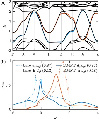
Figure 5: (a) Band structure of LaNiO₂ from DFT (black) and our two-orbital model ($d_{x^{2}-y^{2}}$ in blue and $\textrm{h-}d_{z^{2}}$ in red). (b) Local spectral functions from (a) (bare) and DMFT ($U\!=\!3.1$, $J\!=\!0.7$). The occupancy per orbital is given in brackets.

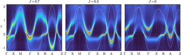
Figure 6: Momentum-resolved spectral function $\mathcal{A}({{\bm{k}},\omega})$ of LaNiO₂ at variable $J$ and fixed $U\!=\!3.1$ (with a broadening of $0.1$ for plotting purposes). At $J\!\lesssim\!0.3$, $n_{z^{2}}$ has decreased sufficiently so that the $\Gamma$ pocket is lifted above $\omega\!=\!0$. White lines show the bare Wannier bands.

We now move on to a material-oriented setting and study the normal state of LaNiO₂. While different models for LaNiO₂ with a variable number of orbitals have been constructed, we here consider a minimal two-orbital model Sakakibara et al. (2020); Hepting et al. (2020); Adhikary et al. (2020); Wan et al. (2021); Kang and Kotliar (2021) at fixed occupancy $N\!=\!1$ (quarter-filling). Evidently, this constitutes a strong simplification compared to more realistic simulations of infinite-layer nickelates and can be seen as a minimal extension beyond a model based on only the $d_{x^{2}-y^{2}}$ orbital. Indeed, our model allows us to investigate to what extent orbital fluctuations and Hund physics in this compound persist when treated in a pure two-orbital description.

Henceforth, our unit of energy is $\mathrm{eV}$ and $J\!\equiv\!J_{\mathrm{HK}}$. We employ the two-orbital model of LaNiO₂ from Ref. Kang and Kotliar (2021) (see their Fig. S16) constructed from the DFT band structure in a small energy window of roughly $[-1.5,2.5]$ w.r.t. the Fermi level. Differently from other models Sakakibara et al. (2020); Hepting et al. (2020); Adhikary et al. (2020); Wan et al. (2021), we thereby choose two Ni-centered Wannier functions Kang and Kotliar (2021). Next to the strongly correlated orbital of mostly Ni $d_{x^{2}-y^{2}}$ character, we have a weakly correlated hybridized orbital of both Ni and La $d_{3z^{2}-r^{2}}$ character ($d_{z^{2}}$ for short), acting as the self-doping band. We label this orbital $\textrm{h-}d_{z^{2}}$ (hybridized $d_{z^{2}}$) to emphasize that it is not equivalent to an orbital of dominant Ni $d_{z^{2}}$ character (as obtained, e.g., from a large energy-window construction). Our model has a sizable crystal-field splitting between the $d_{x^{2}-y^{2}}$ and $\textrm{h-}d_{z^{2}}$ orbital of $\Delta\!\approx\!-0.8$. We will see that, in the quarter-filled two-orbital system, this large $|\Delta|$ leads to a large orbital polarization between the $d_{x^{2}-y^{2}}$ and $\textrm{h-}d_{z^{2}}$ orbital (the former almost half-filled, the latter almost empty), suppressing orbital fluctuations and Hund-metal characteristics.

Figure 5(a) displays the band structure of LaNiO₂ from DFT and from our two-orbital model. The model reproduces the original band structure quantitatively within, say, $[-0.5,1]$, and qualitatively within $[-1,2]$. Statements about LaNiO₂ at larger energies are evidently not captured by the model. We choose $U\!=\!3.1$ and $J\!=\!0.7$, as in the narrow energy-window setting of Ref. Karp et al. (2020a). Figure 5(b) shows the local spectral functions $\mathcal{A}_{\mathrm{loc}}$ from the bare model (dashed lines) and from DMFT (full lines). As can be readily seen, correlations (incorporated via DMFT) change the spectrum sifnificantly. Especially in the $d_{x^{2}-y^{2}}$ orbital, the quasiparticle peak is sharpened and notable Hubbard side bands emerge. We indicate the occupancy per orbital $n_{m}$ in brackets. The orbital polarization ($n_{x^{2}-y^{2}}\!\gg\!n_{z^{2}}$) is slightly decreased by correlations but still sizable. Since the $\textrm{h-}d_{z^{2}}$ orbital is barely occupied, it is much less correlated ($Z_{z^{2}}\!\gg\!Z_{x^{2}-y^{2}}$). The precise quasiparticle weight of the $d_{x^{2}-y^{2}}$ orbital depends on its proximity to half-filling Si et al. (2020). With $n_{x^{2}-y^{2}}\!=\!0.82$, we find $Z_{x^{2}-y^{2}}\!=\!0.29$, consistently with Fig. S1 of Ref. Si et al. (2020) and somewhat similarly to Ref. Karp et al. (2020a) (there, $Z_{x^{2}-y^{2}}\!=\!0.25$ at $n_{x^{2}-y^{2}}\!=\!0.903$ in a three-orbital setting for NdNiO₂ with the same $U$ and $J$ values as used here).

$J$	$n_{x^{2}-y^{2}}$	$Z_{x^{2}-y^{2}}$	$p_{0,0}$	$p_{1,1/2}$	$p_{2,1}$	$p_{2,0}$	$p_{3,1/2}$	$p_{4,0}$
0.7	0.82	0.29	15.5%	69.4%	10.0%	4.7%	0.4%	0
0.3	0.94	0.28	10.7%	78.7%	2.9%	7.6%	0.1%	0
0	0.98	0.27	9.4%	81.3%	0.6%	8.7%	0	0

Table 3: LaNiO₂ results for varying $J$ at $U\!=\!3.1$. Probabilities $p_{N,S^{z}}$ for impurity occupancies at different charge $N$ and spin $S$. Even at $J\!=\!0.7$, the spin triplet state has less weight (10.1%) than in the five-orbital calculation of Ref. Wang et al. (2020a).

We now turn to the effect of Hund’s coupling $J$. At $J\!=\!0$, the large crystal-field splitting would yield an almost depleted $\textrm{h-}d_{z^{2}}$ orbital, whereas large $J$ promotes a large-spin state involving both orbitals. Table 3 confirms this expectation, giving the values for $n_{x^{2}-y^{2}}$ (while $n_{z^{2}}\!=\!1\!-\!n_{x^{2}-y^{2}}$) for $J\!=\!0.7,0.3,0$ at fixed $U\!=\!3.1$. As expected, $Z_{x^{2}-y^{2}}$ is reduced as the orbital approaches half-filling Si et al. (2020). In Fig. 7, showing $\mathcal{A}({{\bm{k}},\omega})$, one can see how the $\Gamma$ pocket is lifted above the Fermi level for sufficiently low $n_{z^{2}}$, realized at $J\!\lesssim\!0.3$. Table 3 also gives the eigenvalues of the impurity density matrix for each symmetry sector (i.e., the valence histogram Shim et al. (2007)). Of particular interest is the weight $p_{2,1}$ of the high-spin multiorbital state. It strongly decreases with decreasing $J$. However, even at large $J\!=\!0.7$, $p_{2,1}\!=\!10.1\%$ is much smaller than the value in Ref. Wang et al. (2020a), treating LaNiO₂ with five correlated orbitals ($25.9\%$ in their Table II; $Z_{x^{2}-y^{2}}\!=\!0.36$ in their Table I is comparable to ours).

Next, we scrutinize to what extent dynamic correlators of the more correlated $d_{x^{2}-y^{2}}$ orbital are affected by $J$. We present in Fig. 7 the spectral functions, self-energies (real part), and spin and orbital susceptibilities for $J\!\in\!\{0.7,0.3,0\}$ at $U\!=\!3.1$. We also include (as a black line) results from a one-shot one-orbital calculation, where we kept $U\!=\!3.1$ and took the hybridization function for the $d_{x^{2}-y^{2}}$ orbital from the two-orbital $J\!=\!0.7$ calculation. For all values of $J$ and even the one-orbital calculation, the low-energy behavior is very similar. This includes the shape of the quasiparticle peak in $\mathcal{A}$, the slope in $\mathrm{Re}\!\;\Sigma$, and the peak position of $\chi^{\prime\prime}_{\mathrm{sp}}$ (as a measure for $T^{\mathrm{K}}_{\mathrm{sp}}$). Note that the peak of $\chi^{\prime\prime}_{\mathrm{orb}}$ occurs at higher energies than that of $\chi^{\prime\prime}_{\mathrm{sp}}$ even at $J\!=\!0$ (trivial SOS due to large $|\Delta|$) and shifts only slightly to higher energies with increasing $J$. This comparison demonstrates that the effect $J$ in our two-orbital model for LaNiO₂ is mostly restricted to the orbital occupancies. Indeed, as a one-orbital calculation with the appropriate input suffices to reproduce the relevant quantities at low energies Karp et al. (2020a), we confirm the interpretation that the low-energy physics of LaNiO₂ is that of a single-band Hubbard model with an appropriate self-doping (provided by other orbitals) Karp et al. (2020a); Kitatani et al. (2020).

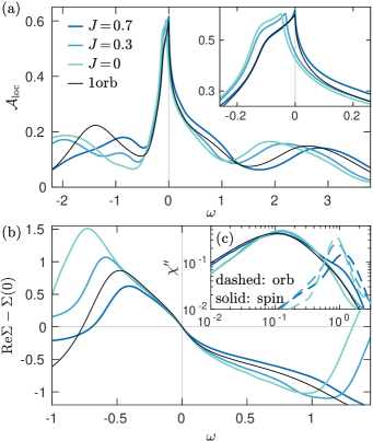
Figure 7: (a) Spectral functions and (b) real part of self-energies of the $d_{x^{2}-y^{2}}$ orbital; (c) susceptibilities. The results stem from variable $J$ in the two-orbital model of LaNiO₂ and from a one-shot one-orbital (1orb) calculation starting from the two-orbital solution at $J\!=\!0.7$.

Finally, Fig. 8 shows the NRG flow diagram of our two-orbital model of LaNiO₂ at $U\!=\!3.1$, $J\!=\!0.7$. The left panel resembles the rightmost panel in Fig. 4 in that the size of the crystal-field splitting prevents 2SKS. As a computational experiment, we add to our model an extra crystal field to achieve $\Delta\!=\!0$, thus compensating the original splitting. The corresponding flow diagram (right panel in Fig. 8) now has an intermediate region with a spin-triplet lowest-energy state that screens the orbital momentum. This confirms that it is indeed the crystal-field splitting (or equivalently the polarization) that suppresses low-energy Hund physics in LaNiO₂.

Figure 8: NRG flow diagram for LaNiO₂ in the original setting $\Delta\!\neq\!0$ and from a computational experiment where we manually set $\Delta\!=\!0$.

IV Conclusion

We studied Hund physics in idealized two- and three-orbital systems and in a two-orbital model of LaNiO₂. Using NRG as DMFT impurity solver allowed us to examine high-resolution real-frequency spectra and the NRG flow from high to low energies. The latter was found to be a uniquely adequate tool to check for 2SKS, the arguably most fascinating mechanism behind the SOS of Kondo scales—a hallmark of Hund metals.

First, we focused on orbital-symmetric models and compared three cases of $N$ electrons in $M$ orbitals: $(M,N)\!\in\!\{(3,2),(3,1),(2,1)\}$. As indications of Hund physics, we examined (i) the Janus effect in $Z(U,J)$, (ii) the SOS of Kondo scales, (iii) 2SKS in the RG flow with an intermediate orbital-singlet spin-triplet state, and (iv) the orbital-resonance shoulder in $\mathcal{A}$ and the corresponding inverted slope in $\mathrm{Re}\!\;\Sigma$ (for orbital-symmetric models). The case $(M,N)\!=\!(3,2)$ is known to prominently feature Hund physics: Since $J$ splits the atomic ground-state manifold, $Z$ and $T^{\mathrm{K}}_{\mathrm{sp}}$ decrease drastically with $J$, enabling (i) a clear Janus effect and (ii) wide SOS. (iii) The RG flow has a wide energy window between $T^{\mathrm{K}}_{\mathrm{sp}}$ and $T^{\mathrm{K}}_{\mathrm{orb}}$ dominated by an orbital-singlet spin-triplet state, and (iv) $\mathcal{A}$ shows a pronounced shoulder ($\mathrm{Re}\!\;\Sigma$ an inverted slope).

Since $J$ does not affect the atomic ground state for $N=1$, properties (i) and (ii) are not very pronounced in the two cases $(M,N)\!\in\!\{(3,1),(2,1)\}$. For $(M,N)\!=\!(3,1)$, one does not observe any signs of properties (iii) and (iv) either. However, for $(M,N)\!=\!(2,1)$, even though the window between $T^{\mathrm{K}}_{\mathrm{sp}}$ and $T^{\mathrm{K}}_{\mathrm{orb}}$ is relatively small (slightly larger than a decade), one can distinguish an orbital-singlet spin-triplet state as the lowest-energy state. Similarly, one can distinguish a weak shoulder in $\mathcal{A}$ (inverted slope in $\mathrm{Re}\!\;\Sigma$). Thereby, we substantiate the notion of a weak Hund metal for $(M,N)\!=\!(2,1)$ Ryee et al. (2021). The RG flow reveals that 2SKS and the intermediate orbital-singlet spin-triplet state formed by binding a bath electron is facilitated by $N\!=\!M\!-\!1$ (i.e., one-charge proximity to half-filling, independent of $N$), while it is unlikely for $N\!=\!M\!-\!2$ (where two bath electrons would be required to form an orbital singlet).

We then studied the effect of a crystal-field splitting $\Delta$ and showed that 2SKS is obviated if $|\Delta|\!\gtrsim\!T^{\mathrm{K}}_{\mathrm{orb}}(\Delta\!=\!0)/2$. In systems with strongly broken orbital symmetry, 2SKS does not go hand in hand with SOS or the shoulder in $\mathcal{A}$ (inverted slope in $\mathrm{Re}\!\;\Sigma$): On the one hand, for large $|\Delta|$, $\chi^{\prime\prime}_{\mathrm{orb}}$ peaks at the bare parameter $|\Delta|$ due to atomic quenching of orbital fluctuations (and not dynamic Kondo screening). On the other hand, the shoulder in $\mathcal{A}$ then changes in nature from an orbital-resonance shoulder to a separate doublon-holon peak Kugler et al. (2019).

An important next step is to elucidate how 2SKS and the intermediate orbital-singlet spin-triplet state are reflected in observables; one candidate are fractional power laws at intermediate frequencies in local susceptibilities Walter et al. (2020); Wang et al. (2020b). Here, our observation of 2SKS in a quarter-filled two-orbital model is helpful as it constitutes a conceptually and numerically simpler setting than the previously known case $(M,N)\!=\!(3,2)$. We thus suggest a similar study as in Refs. Walter et al. (2020); Wang et al. (2020b), using a generalized Kondo model to manually increase the intermediate energy window between $T^{\mathrm{K}}_{\mathrm{sp}}$ and $T^{\mathrm{K}}_{\mathrm{orb}}$, but for $(M,N)\!=\!(2,1)$.

Second, we analyzed a two-orbital model of LaNiO₂, containing the strongly correlated $d_{x^{2}-y^{2}}$ orbital and a weakly correlated hybridized orbital of $d_{z^{2}}$ symmetry (not equivalent to the Ni $d_{z^{2}}$ orbital of a large energy-window construction). Our aim was to study a minimal setting in which to test Hund physics while undoubtedly compromising on the degree of realism. In particular, the frozen charge of one electron in the low-energy two-band window is a significant simplification—it is known that different orbital occupancies in different models lead to variable outcomes on quantities like $Z_{x^{2}-y^{2}}$.

In our quarter-filled two-orbital model, $J$ mainly affects the orbital occupancies while low-energy Hund physics are suppressed by the large $|\Delta|\!\approx\!0.8\,\mathrm{eV}$. This confirms the interpretation that the low-energy physics of LaNiO₂ is that of a single-band Hubbard model with an appropriate self-doping (provided by other orbitals) Karp et al. (2020a); Kitatani et al. (2020). Nevertheless, we showed that multiorbital effects in our two-orbital model can be revived by counteracting the crystal-field splitting, thus reducing the orbital polarization. A first test within DFT showed that positive strain along the $c$ direction at constant volume of the unit cell (thus decreasing $c/a$, where $a\!=\!b$, and $c/a\!\approx\!0.87$ in the pristine structure) decreases the energy splitting between the two orbitals. It would be interesting to realize similar effects in experiment and thereby induce low-energy Hund physics.

Appendix A Comparing quasiparticle weights

Figure 9 shows that $Z$ depends very similarly on $U$ and $J$ for both the DN and the HK interaction Hamiltonians. For the closest connection between both situations, we match the intraorbital interaction $U$ as well as the atomic gap $\Delta_{\mathrm{at}}\!=\!U^{\prime}\!-\!J$. Next to $U\!\equiv\!U_{\mathrm{DN}}\!=\!U_{\mathrm{HK}}$, this leads to the relation

$$U^{\prime}_{\mathrm{DN}}\!-\!J_{\mathrm{DN}}=U^{\prime}_{\mathrm{HK}}\!-\!J_{\mathrm{HK}}\Leftrightarrow U\!-\!2J_{\mathrm{DN}}=U\!-\!3J_{\mathrm{HK}}.$$ (4)

This simplifies to $J_{\mathrm{HK}}\!=\!\frac{2}{3}J_{\mathrm{DN}}$, and $J_{\mathrm{DN}}\!=\!\frac{1}{3}U\Rightarrow J_{\mathrm{HK}}\!=\!\frac{2}{9}U$.

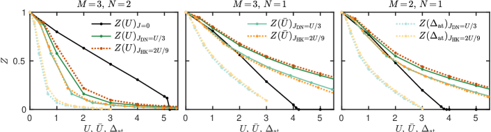
Figure 9: Quasiparticle weight $Z$ as a function of $U$, $\bar{U}$, or $\Delta_{\mathrm{at}}$, analogous to Fig. 2(a), compared between the DN and the HK Hamiltonians. The behavior is qualitatively very similar for both Hamiltonians. Compared as a function of $\bar{U}$ or $\Delta_{\mathrm{at}}$, the results even agree on a quantitative level.

Appendix B Operators and interaction Hamiltonians

In a multiorbital system, we have the (local) charge and spin operators

$$N =\sum_{m\sigma}d^{\dagger}_{m\sigma}d_{m\sigma},\quad{\bm{S}}=\tfrac{1}{2}\sum_{m\sigma\sigma^{\prime}}d^{\dagger}_{m\sigma}{\bm{\sigma}}_{\sigma\sigma^{\prime}}d_{m\sigma^{\prime}},$$ (5)

with the Pauli matrices ${\bm{\sigma}}$. For $M\!=\!3$, specifically, we have

$$T_{a} =\tfrac{1}{2}\sum_{mm^{\prime}\sigma}d^{\dagger}_{m\sigma}\lambda^{a}_{mm^{\prime}}d_{m^{\prime}\sigma},$$ (6)

$$L_{m} =\mathrm{i}\sum_{m^{\prime}m^{\prime\prime}\sigma}\epsilon_{mm^{\prime}m^{\prime\prime}}d^{\dagger}_{m^{\prime}\sigma}d_{m^{\prime\prime}\sigma}$$ (7)

as orbital operators. Here, $T_{a}$ ($a=1,\kern-1.49994pt.\kern-0.50003pt.\kern-0.50003pt.,8$) applies to SU(3) symmetry and uses the Gell-Mann matrices $\lambda^{a}$, while $L_{m}$ ($m=1,\kern-1.49994pt.\kern-0.50003pt.\kern-0.50003pt.,3$) applies to SO(3) symmetry and uses the Levi-Civita symbol $\epsilon_{mm^{\prime}m^{\prime\prime}}$. For $M=2$, one can replace the Gell-Mann matrices by the Pauli matrices for SU(2) orbital symmetry, and one can use $L\equiv L_{3}$ for SO(2) symmetry.

From these operators, we can build the quartic terms

$$N^{2},\quad{\bm{S}}^{2},\quad{\bm{T}}^{2},\quad{\bm{L}}^{2}.$$ (8)

In the $S^{z}$ basis, one often refers to the following interactions as density-density (intraorbital, interorbital opposite-spin, same-spin), spin-flip, and pair-hopping terms, respectively:

$$H^{(1)}_{\mathrm{dd}} =\!\sum_{m}n_{m\uparrow}n_{m\downarrow},\quad H^{(2)}_{\mathrm{dd}}=\!\sum_{m\neq m^{\prime}}n_{m\uparrow}n_{m^{\prime}\downarrow},$$

$$H^{(3)}_{\mathrm{dd}} =\!\!\sum_{m<m^{\prime},\sigma}\!\!\!\!n_{m\sigma}n_{m^{\prime}\sigma},\quad H_{\mathrm{sf}}=-\!\!\sum_{m\neq m^{\prime}}\!d^{\dagger}_{m\uparrow}d_{m\downarrow}d^{\dagger}_{m^{\prime}\downarrow}d_{m^{\prime}\uparrow},$$

$$H_{\mathrm{ph}} =\!\sum_{m\neq m^{\prime}}\!d^{\dagger}_{m\uparrow}d^{\dagger}_{m\downarrow}d_{m^{\prime}\downarrow}d_{m^{\prime}\uparrow}.$$ (9)

Their relation to the terms in Eq. (8), as derived below, is

$$\tfrac{1}{2}N(N\!-\!1)=H^{(1)}_{\mathrm{dd}}+H^{(2)}_{\mathrm{dd}}+H^{(3)}_{\mathrm{dd}},$$ (10a)

$${\bm{S}}^{2}+\tfrac{1}{4}N^{2}-N=-H^{(1)}_{\mathrm{dd}}+H^{(3)}_{\mathrm{dd}}-H_{\mathrm{sf}},$$ (10b)

$${\bm{T}}^{2}+\tfrac{1}{2M}N^{2}-\tfrac{M}{2}N=H^{(1)}_{\mathrm{dd}}-H^{(3)}_{\mathrm{dd}}+H_{\mathrm{sf}},$$ (10c)

$$\tfrac{1}{2}[{\bm{L}}^{2}-(M\!-\!1)N]=-H^{(3)}_{\mathrm{dd}}+H_{\mathrm{sf}}-H_{\mathrm{ph}}.$$ (10d)

Evidently, ${\bm{T}}^{2}$ is linearly dependent on $N^{2}$, $N$, and ${\bm{S}}^{2}$. We abbreviate Eqs. (10b)–(10d) as $\tilde{{\bm{S}}}^{2}$, $\tilde{{\bm{T}}}^{2}$, and $\tfrac{1}{2}\tilde{{\bm{L}}}^{2}$, respectively.

The combinations forming the generalized Kanamori (GK) and the HK Hamiltonians are (cf. Ref. Georges et al. (2013) for $M=3$)

$$H_{\mathrm{GK}} =\frac{3U^{\prime}-U}{2}\tfrac{1}{2}N(N\!-\!1)+(U^{\prime}-U){\bm{S}}^{2}$$

$$\ +(U^{\prime}-U+J)\tfrac{1}{2}{\bm{L}}^{2}+\big{[}\tfrac{1+2M}{4}(U-U^{\prime})+\tfrac{1-M}{2}J\big{]}N$$

$$=U^{\prime}\tfrac{1}{2}N(N\!-\!1)+(U^{\prime}-U)\tilde{{\bm{S}}}^{2}+(U^{\prime}-U+J)\tfrac{1}{2}\tilde{{\bm{L}}}^{2}$$

$$=UH^{(1)}_{\mathrm{dd}}+U^{\prime}H^{(2)}_{\mathrm{dd}}+(U^{\prime}-J)H^{(3)}_{\mathrm{dd}}+JH_{\mathrm{sf}}$$

$$\ +(U-U^{\prime}-J)H_{\mathrm{ph}},$$ (11)

which, for $U^{\prime}=U-2J$, simplifies to

$$H_{\mathrm{HK}} =(U-3J)\tfrac{1}{2}N(N\!-\!1)-2J{\bm{S}}^{2}-J\tfrac{1}{2}{\bm{L}}^{2}+\tfrac{2+M}{2}JN$$

$$=U^{\prime}\tfrac{1}{2}N(N-1)-2J\tilde{{\bm{S}}}^{2}-J\tfrac{1}{2}\tilde{{\bm{L}}}^{2}$$

$$=UH^{(1)}_{\mathrm{dd}}+U^{\prime}H^{(2)}_{\mathrm{dd}}+(U^{\prime}\!-\!J)H^{(3)}_{\mathrm{dd}}+J(H_{\mathrm{sf}}\!+\!H_{\mathrm{ph}}).$$ (12)

The DN Hamiltonian is given by Georges et al. (2013)

$$H_{\mathrm{DN}} =(U-\tfrac{3}{2}J)\tfrac{1}{2}N(N\!-\!1)-J{\bm{S}}^{2}+\tfrac{3}{4}JN$$

$$=(U-J)\tfrac{1}{2}N(N\!-\!1)-J\tilde{{\bm{S}}}^{2}$$

$$=(U-J)\tfrac{1}{2}N(N\!-\!1)-2J\tilde{{\bm{S}}}^{2}-J\tilde{{\bm{T}}}^{2}$$

$$=UH^{(1)}_{\mathrm{dd}}+(U\!-\!J)H^{(2)}_{\mathrm{dd}}+(U\!-\!2J)H^{(3)}_{\mathrm{dd}}+JH_{\mathrm{sf}}.$$ (13)

The second-to-last row is a trivial rewriting, emphasizing the similarity to the HK Hamiltonian with prefactors $-2J$ and $-J$ in front of the spin and orbital operators squared, respectively.

To derive Eqs. (10), we first normal-order the interactions:

$$N^{2} =\sum_{\alpha\alpha^{\prime}}d^{\dagger}_{\alpha}d_{\alpha}d^{\dagger}_{\alpha^{\prime}}d_{\alpha^{\prime}}=\sum_{\alpha\alpha^{\prime}}d^{\dagger}_{\alpha}d^{\dagger}_{\alpha^{\prime}}d_{\alpha^{\prime}}d_{\alpha}+N,$$ (14)

where $\alpha\!=\!(m,\sigma)$. Further, we have

$${\bm{S}}^{2} =\tfrac{1}{4}\sum_{\begin{subarray}{c}m\sigma\sigma^{\prime}\\ \tilde{m}\tilde{\sigma}\tilde{\sigma}^{\prime}\end{subarray}}d^{\dagger}_{m\sigma}d_{m\sigma^{\prime}}d^{\dagger}_{\tilde{m}\tilde{\sigma}}d_{\tilde{m}\tilde{\sigma}^{\prime}}{\bm{\sigma}}_{\sigma\sigma^{\prime}}\cdot{\bm{\sigma}}_{\tilde{\sigma}\tilde{\sigma}^{\prime}}.$$ (15)

Using ${\bm{\sigma}}_{\sigma\sigma^{\prime}}\cdot{\bm{\sigma}}_{\tilde{\sigma}\tilde{\sigma}^{\prime}}=2\delta_{\sigma\tilde{\sigma}^{\prime}}\delta_{\sigma^{\prime}\tilde{\sigma}}-\delta_{\sigma\sigma^{\prime}}\delta_{\tilde{\sigma}\tilde{\sigma}^{\prime}}$, we get

$${\bm{S}}^{2} =\tfrac{1}{2}\sum_{mm^{\prime}\sigma}d^{\dagger}_{m\sigma}d_{m\sigma^{\prime}}d^{\dagger}_{m^{\prime}\sigma^{\prime}}d_{m^{\prime}\sigma}-\tfrac{1}{4}N^{2}.$$ (16)

Then, $d_{m\sigma^{\prime}}d^{\dagger}_{m^{\prime}\sigma^{\prime}}=-d^{\dagger}_{m^{\prime}\sigma^{\prime}}d_{m\sigma^{\prime}}+\delta_{mm^{\prime}}$ yields

$${\bm{S}}^{2}=\tfrac{1}{2}\sum_{mm^{\prime}\sigma\sigma^{\prime}}d^{\dagger}_{m\sigma}d^{\dagger}_{m^{\prime}\sigma^{\prime}}d_{m^{\prime}\sigma}d_{m\sigma^{\prime}}+N-\tfrac{1}{4}N^{2}.$$ (17)

In the case of $\mathrm{SU}(2)$ orbital symmetry, one finds

$${\bm{T}}^{2} \overset{M=2}{=}-\tfrac{1}{2}\sum_{mm^{\prime}\sigma\sigma^{\prime}}d^{\dagger}_{m\sigma}d^{\dagger}_{m^{\prime}\sigma^{\prime}}d_{m^{\prime}\sigma}d_{m\sigma^{\prime}}+N-\tfrac{1}{4}N^{2}$$ (18)

by a simple replacement of $m\!\leftrightarrow\!\sigma$. For $M\!=\!3$, we have

$${\bm{T}}^{2} =\tfrac{1}{4}\sum_{\begin{subarray}{c}mm^{\prime}\sigma\\ \tilde{m}\tilde{m}^{\prime}\tilde{\sigma}\end{subarray}}d^{\dagger}_{m\sigma}d_{m^{\prime}\sigma}d^{\dagger}_{\tilde{m}\tilde{\sigma}}d_{\tilde{m}^{\prime}\tilde{\sigma}}\sum_{a}\lambda_{mm^{\prime}}\lambda_{\tilde{m}\tilde{m}^{\prime}}.$$ (19)

Using $\sum_{a}\lambda_{mm^{\prime}}\lambda_{\tilde{m}\tilde{m}^{\prime}}=2\delta_{m\tilde{m}^{\prime}}\delta_{m^{\prime}\tilde{m}}-\tfrac{2}{3}\delta_{mm^{\prime}}\delta_{\tilde{m}\tilde{m}^{\prime}}$, we get

$${\bm{T}}^{2} =\tfrac{1}{2}\sum_{mm^{\prime}\sigma\sigma^{\prime}}d^{\dagger}_{m\sigma}d_{m^{\prime}\sigma}d^{\dagger}_{m^{\prime}\sigma^{\prime}}d_{m\sigma^{\prime}}-\tfrac{1}{6}N^{2}.$$ (20)

We commute $d_{m^{\prime}\sigma}d^{\dagger}_{m^{\prime}\sigma^{\prime}}=-d^{\dagger}_{m^{\prime}\sigma^{\prime}}d_{m^{\prime}\sigma}+\delta_{\sigma\sigma^{\prime}}$ to obtain

$${\bm{T}}^{2} =-\tfrac{1}{2}\sum_{mm^{\prime}\sigma\sigma^{\prime}}d^{\dagger}_{m\sigma}d^{\dagger}_{m^{\prime}\sigma^{\prime}}d_{m^{\prime}\sigma}d_{m\sigma^{\prime}}+\tfrac{3}{2}N-\tfrac{1}{6}N^{2}.$$ (21)

We can thus summarize both cases $M\!\in\!\{2,3\}$ as

$${\bm{T}}^{2} =-\tfrac{1}{2}\sum_{mm^{\prime}\sigma\sigma^{\prime}}d^{\dagger}_{m\sigma}d^{\dagger}_{m^{\prime}\sigma^{\prime}}d_{m^{\prime}\sigma}d_{m\sigma^{\prime}}+\tfrac{M}{2}N-\tfrac{1}{2M}N^{2}.$$ (22)

For $\mathrm{SO}(M)$ orbital symmetry, we have

$${\bm{L}}^{2} =-\sum_{\begin{subarray}{c}kl\sigma\\ k^{\prime}l^{\prime}\sigma^{\prime}\end{subarray}}\sum_{m}\epsilon_{mkl}\epsilon_{mk^{\prime}l^{\prime}}d^{\dagger}_{k\sigma}d_{l\sigma}d^{\dagger}_{k^{\prime}\sigma^{\prime}}d_{l^{\prime}\sigma^{\prime}},$$ (23)

where $m,k,l,k^{\prime},l^{\prime}\in\{1,2,3\}$ for $M=3$ and $k,l,k^{\prime},l^{\prime}\in\{1,2\}$ while $m=3$ for $M=2$. In both cases, we can use $\sum_{m}\epsilon_{mkl}\epsilon_{mk^{\prime}l^{\prime}}=\delta_{kk^{\prime}}\delta_{ll^{\prime}}-\delta_{kl^{\prime}}\delta_{lk^{\prime}}$ to get

$${\bm{L}}^{2} =\sum_{kl\sigma\sigma^{\prime}}(d^{\dagger}_{k\sigma}d_{l\sigma}d^{\dagger}_{l\sigma^{\prime}}d_{k\sigma^{\prime}}-d^{\dagger}_{k\sigma}d_{l\sigma}d^{\dagger}_{k\sigma^{\prime}}d_{l\sigma^{\prime}}).$$ (24)

Via $d_{l\sigma}d^{\dagger}_{l\sigma^{\prime}}=-d^{\dagger}_{l\sigma^{\prime}}d_{l\sigma}+\delta_{\sigma\sigma^{\prime}}$ and $d_{l\sigma}d^{\dagger}_{k\sigma^{\prime}}=-d^{\dagger}_{k\sigma^{\prime}}d_{l\sigma}+\delta_{kl}\delta_{\sigma\sigma^{\prime}}$, we find

$${\bm{L}}^{2} =\sum_{mm^{\prime}\sigma\sigma^{\prime}}(d^{\dagger}_{m\sigma}d^{\dagger}_{m^{\prime}\sigma^{\prime}}d_{m\sigma^{\prime}}d_{m^{\prime}\sigma}-d^{\dagger}_{m\sigma}d^{\dagger}_{m\sigma^{\prime}}d_{m^{\prime}\sigma^{\prime}}d_{m^{\prime}\sigma})$$

$$\ +(M-1)N.$$ (25)

Now, Eq. (14) is simplified, after dividing $\sum_{mm^{\prime}\sigma\sigma^{\prime}}$ into $\sum_{m=m^{\prime},\sigma\neq\sigma^{\prime}}$, $\sum_{m\neq m^{\prime},\sigma=\sigma^{\prime}}$, and $\sum_{m\neq m^{\prime},\sigma\neq\sigma^{\prime}}$, as

$$\tfrac{1}{2}N(N\!-\!1) =\tfrac{1}{2}\sum_{mm^{\prime}\sigma\sigma^{\prime}}d^{\dagger}_{m\sigma}d^{\dagger}_{m^{\prime}\sigma^{\prime}}d_{m^{\prime}\sigma^{\prime}}d_{m\sigma}$$

$$=H^{(1)}_{\mathrm{dd}}+H^{(2)}_{\mathrm{dd}}+H^{(3)}_{\mathrm{dd}}.$$ (26)

Similarly, Eqs. (17), (22), and (25) give

$$\tilde{{\bm{S}}}^{2} =-\tilde{{\bm{T}}}^{2}=\tfrac{1}{2}\!\!\sum_{mm^{\prime}\sigma\sigma^{\prime}}\!\!d^{\dagger}_{m\sigma}d^{\dagger}_{m^{\prime}\sigma^{\prime}}d_{m^{\prime}\sigma}d_{m\sigma^{\prime}}$$

$$=-H^{(1)}_{\mathrm{dd}}+H^{(3)}_{\mathrm{dd}}-H_{\mathrm{sf}},$$ (27)

$$\tfrac{1}{2}\tilde{{\bm{L}}}^{2} =\tfrac{1}{2}\sum_{mm^{\prime}\sigma\sigma^{\prime}}d^{\dagger}_{m\sigma}(d^{\dagger}_{m^{\prime}\sigma^{\prime}}d_{m\sigma^{\prime}}-d^{\dagger}_{m\sigma^{\prime}}d_{m^{\prime}\sigma^{\prime}})d_{m^{\prime}\sigma}$$

$$=-H^{(3)}_{\mathrm{dd}}+H_{\mathrm{sf}}-H_{\mathrm{ph}}.$$ (28)

Thus, Eqs. (10) are derived. For completeness, we mention that ${\bm{S}}^{2}$ can be decomposed into $\sum_{m}{\bm{S}}_{m}^{2}\!=\!-\tfrac{3}{2}H^{(1)}_{\mathrm{dd}}+\tfrac{3}{4}N$ and $2\sum_{m<m^{\prime}}{\bm{S}}_{m}\cdot{\bm{S}}_{m^{\prime}}\!=\!-\tfrac{1}{2}H^{(2)}_{\mathrm{dd}}+\tfrac{1}{2}H^{(3)}_{\mathrm{dd}}-H_{\mathrm{sf}}$.

References

- Yin et al. (2011) Z. P. Yin, K. Haule, and G. Kotliar, Nat. Mater. 10, 932 (2011).
- Georges et al. (2013) A. Georges, L. de’ Medici, and J. Mravlje, Annu. Rev. Condens. Matter Phys. 4, 137 (2013).
- Jang et al. (2021) B. G. Jang, G. Han, I. Park, D. Kim, Y. Y. Koh, Y. Kim, W. Kyung, H.-D. Kim, C.-M. Cheng, K.-D. Tsuei, K. D. Lee, N. Hur, J. H. Shim, C. Kim, and G. Kotliar, Nat. Commun. 12, (2021).
- (4) I. Park, B. G. Jang, D. W. Kim, J. H. Shim, and G. Kotliar, arXiv:2309.15392 .
- Li et al. (2019) D. Li, K. Lee, B. Y. Wang, M. Osada, S. Crossley, H. R. Lee, Y. Cui, Y. Hikita, and H. Y. Hwang, Nature 572, 624 (2019).
- Georges et al. (1996) A. Georges, G. Kotliar, W. Krauth, and M. J. Rozenberg, Rev. Mod. Phys. 68, 13 (1996).
- Kotliar et al. (2006) G. Kotliar, S. Y. Savrasov, K. Haule, V. S. Oudovenko, O. Parcollet, and C. A. Marianetti, Rev. Mod. Phys. 78, 865 (2006).
- Karp et al. (2020a) J. Karp, A. S. Botana, M. R. Norman, H. Park, M. Zingl, and A. Millis, Phys. Rev. X 10, 021061 (2020a).
- Lechermann (2020a) F. Lechermann, Phys. Rev. B 101, 081110 (2020a).
- Gu et al. (2020) Y. Gu, S. Zhu, X. Wang, J. Hu, and H. Chen, Commun. Phys. 3, (2020).
- Ryee et al. (2020) S. Ryee, H. Yoon, T. J. Kim, M. Y. Jeong, and M. J. Han, Phys. Rev. B 101, 064513 (2020).
- Si et al. (2020) L. Si, W. Xiao, J. Kaufmann, J. M. Tomczak, Y. Lu, Z. Zhong, and K. Held, Phys. Rev. Lett. 124, 166402 (2020).
- Kitatani et al. (2020) M. Kitatani, L. Si, O. Janson, R. Arita, Z. Zhong, and K. Held, npj Quantum Mater. 5, (2020).
- Lechermann (2020b) F. Lechermann, Phys. Rev. X 10, 041002 (2020b).
- Leonov et al. (2020) I. Leonov, S. L. Skornyakov, and S. Y. Savrasov, Phys. Rev. B 101, 241108 (2020).
- Wang et al. (2020a) Y. Wang, C.-J. Kang, H. Miao, and G. Kotliar, Phys. Rev. B 102, 161118 (2020a).
- Kang and Kotliar (2021) C.-J. Kang and G. Kotliar, Phys. Rev. Lett. 126, 127401 (2021).
- Kang et al. (2023) B. Kang, C. Melnick, P. Semon, S. Ryee, M. J. Han, G. Kotliar, and S. Choi, npj Quantum Mater. 8 (2023), 10.1038/s41535-023-00568-5.
- Ryee et al. (2021) S. Ryee, M. J. Han, and S. Choi, Phys. Rev. Lett. 126, 206401 (2021).
- Gull et al. (2011) E. Gull, A. J. Millis, A. I. Lichtenstein, A. N. Rubtsov, M. Troyer, and P. Werner, Rev. Mod. Phys. 83, 349 (2011).
- Choi et al. (2019) S. Choi, P. Semon, B. Kang, A. Kutepov, and G. Kotliar, Comput. Phys. Commun. 244, 277 (2019).
- Bulla et al. (2008) R. Bulla, T. A. Costi, and T. Pruschke, Rev. Mod. Phys. 80, 395 (2008).
- Sakakibara et al. (2020) H. Sakakibara, H. Usui, K. Suzuki, T. Kotani, H. Aoki, and K. Kuroki, Phys. Rev. Lett. 125, 077003 (2020).
- Hepting et al. (2020) M. Hepting, D. Li, C. J. Jia, H. Lu, E. Paris, Y. Tseng, X. Feng, M. Osada, E. Been, Y. Hikita, Y.-D. Chuang, Z. Hussain, K. J. Zhou, A. Nag, M. Garcia-Fernandez, M. Rossi, H. Y. Huang, D. J. Huang, Z. X. Shen, T. Schmitt, H. Y. Hwang, B. Moritz, J. Zaanen, T. P. Devereaux, and W. S. Lee, Nature Materials 19, 381 (2020).
- Adhikary et al. (2020) P. Adhikary, S. Bandyopadhyay, T. Das, I. Dasgupta, and T. Saha-Dasgupta, Phys. Rev. B 102, 100501 (2020).
- Wan et al. (2021) X. Wan, V. Ivanov, G. Resta, I. Leonov, and S. Y. Savrasov, Phys. Rev. B 103, 075123 (2021).
- Stadler et al. (2015) K. M. Stadler, Z. P. Yin, J. von Delft, G. Kotliar, and A. Weichselbaum, Phys. Rev. Lett. 115, 136401 (2015).
- Ryee et al. (2023) S. Ryee, S. Choi, and M. J. Han, Phys. Rev. Res. 5, 033134 (2023).
- Nomura et al. (2019) Y. Nomura, M. Hirayama, T. Tadano, Y. Yoshimoto, K. Nakamura, and R. Arita, Phys. Rev. B 100, 205138 (2019).
- Liu et al. (2020) Z. Liu, Z. Ren, W. Zhu, Z. Wang, and J. Yang, npj Quantum Mater. 5, (2020).
- Kugler et al. (2020) F. B. Kugler, M. Zingl, H. U. R. Strand, S.-S. B. Lee, J. von Delft, and A. Georges, Phys. Rev. Lett. 124, 016401 (2020).
- Peters et al. (2006) R. Peters, T. Pruschke, and F. B. Anders, Phys. Rev. B 74, 245114 (2006).
- Weichselbaum and von Delft (2007) A. Weichselbaum and J. von Delft, Phys. Rev. Lett. 99, 076402 (2007).
- Weichselbaum (2012a) A. Weichselbaum, Ann. Phys. 327, 2972 (2012a).
- Weichselbaum (2012b) A. Weichselbaum, Phys. Rev. B 86, 245124 (2012b).
- Weichselbaum (2020) A. Weichselbaum, Phys. Rev. Research 2, 023385 (2020).
- Lee and Weichselbaum (2016) S.-S. B. Lee and A. Weichselbaum, Phys. Rev. B 94, 235127 (2016).
- Lee et al. (2017) S.-S. B. Lee, J. von Delft, and A. Weichselbaum, Phys. Rev. Lett. 119, 236402 (2017).
- Kugler (2022) F. B. Kugler, Phys. Rev. B 105, 245132 (2022).
- Mitchell et al. (2014) A. K. Mitchell, M. R. Galpin, S. Wilson-Fletcher, D. E. Logan, and R. Bulla, Phys. Rev. B 89, 121105 (2014).
- Stadler et al. (2016) K. M. Stadler, A. K. Mitchell, J. von Delft, and A. Weichselbaum, Phys. Rev. B 93, 235101 (2016).
- Žitko and Pruschke (2009) R. Žitko and T. Pruschke, Phys. Rev. B 79, 085106 (2009).
- Kugler et al. (2019) F. B. Kugler, S.-S. B. Lee, A. Weichselbaum, G. Kotliar, and J. von Delft, Phys. Rev. B 100, 115159 (2019).
- de’ Medici (2011) L. de’ Medici, Phys. Rev. B 83, 205112 (2011).
- Kugler and Kotliar (2022) F. B. Kugler and G. Kotliar, Phys. Rev. Lett. 129, 096403 (2022).
- Stadler et al. (2019) K. M. Stadler, G. Kotliar, A. Weichselbaum, and J. von Delft, Ann. Phys. 405, 365 (2019).
- Yin et al. (2012) Z. P. Yin, K. Haule, and G. Kotliar, Phys. Rev. B 86, 195141 (2012).
- Aron and Kotliar (2015) C. Aron and G. Kotliar, Phys. Rev. B 91, 041110 (2015).
- de’ Medici et al. (2011) L. de’ Medici, J. Mravlje, and A. Georges, Phys. Rev. Lett. 107, 256401 (2011).
- Iwasawa et al. (2005) H. Iwasawa, Y. Aiura, T. Saitoh, I. Hase, S. I. Ikeda, Y. Yoshida, H. Bando, M. Higashiguchi, Y. Miura, X. Y. Cui, K. Shimada, H. Namatame, and M. Taniguchi, Phys. Rev. B 72, 104514 (2005).
- Mravlje et al. (2011) J. Mravlje, M. Aichhorn, T. Miyake, K. Haule, G. Kotliar, and A. Georges, Phys. Rev. Lett. 106, 096401 (2011).
- Stricker et al. (2014) D. Stricker, J. Mravlje, C. Berthod, R. Fittipaldi, A. Vecchione, A. Georges, and D. van der Marel, Phys. Rev. Lett. 113, 087404 (2014).
- Wadati et al. (2014) H. Wadati, J. Mravlje, K. Yoshimatsu, H. Kumigashira, M. Oshima, T. Sugiyama, E. Ikenaga, A. Fujimori, A. Georges, A. Radetinac, K. S. Takahashi, M. Kawasaki, and Y. Tokura, Phys. Rev. B 90, 205131 (2014).
- Karp et al. (2020b) J. Karp, M. Bramberger, M. Grundner, U. Schollwöck, A. J. Millis, and M. Zingl, Phys. Rev. Lett. 125, 166401 (2020b).
- Walter et al. (2020) E. Walter, K. M. Stadler, S.-S. B. Lee, Y. Wang, G. Kotliar, A. Weichselbaum, and J. von Delft, Phys. Rev. X 10, 031052 (2020).
- Shim et al. (2007) J. H. Shim, K. Haule, and G. Kotliar, Nature 446, 513 (2007).
- Wang et al. (2020b) Y. Wang, E. Walter, S.-S. B. Lee, K. M. Stadler, J. von Delft, A. Weichselbaum, and G. Kotliar, Phys. Rev. Lett. 124, 136406 (2020b).