Iterative Preference Learning from Human Feedback: Bridging Theory and Practice for RLHF under KL-Constraint

Abstract

This paper studies the theoretical framework of the alignment process of generative models with Reinforcement Learning from Human Feedback (RLHF). We consider a standard mathematical formulation, the reverse-KL regularized contextual bandit for RLHF. Despite its widespread practical application, a rigorous theoretical analysis of this formulation remains open. We investigate its behavior in three distinct settings—offline, online, and hybrid—and propose efficient algorithms with finite-sample theoretical guarantees.

Moving towards practical applications, our framework, with a robust approximation of the information-theoretical policy improvement oracle, naturally gives rise to several novel RLHF algorithms. This includes an iterative version of the Direct Preference Optimization (DPO) algorithm for online settings, and a multi-step rejection sampling strategy for offline scenarios. Our empirical evaluations on real-world alignment experiment of large language model demonstrate that these proposed methods significantly surpass existing strong baselines, such as DPO and Rejection Sampling Optimization (RSO), showcasing the connections between solid theoretical foundations and their powerful practical implementations.

tcb@breakable

1 Introduction

Reinforcement Learning from Human Feedback (RLHF) (Christiano et al., 2017; Ziegler et al., 2019) has emerged as a powerful paradigm to align modern generative models like Large Language Models (LLMs) and diffusion models with human values and preferences. This approach has shown significant effectiveness in applications such as ChatGPT (OpenAI, 2023), Claude (Anthropic, 2023), Bard (Google, 2023), and LLaMA2 (Touvron et al., 2023), by making the built AI system helpful, harmless, honest and controllable (Ouyang et al., 2022; Bai et al., 2022a).

Despite its effectiveness, RLHF’s implementation often involves ad-hoc practices and extensive algorithmic tuning in the entire pipeline, including preference data collection (it is hard to select representative humans (Bai et al., 2022a), larger language models (Wang et al., 2024) or program compiler (Wang et al., 2023b) to provide feedback), preference/reward modeling (reward misspecification and misgeneralization (Hong et al., 2022; Gao et al., 2023)), and model optimization (instability of training (Choshen et al., 2019) and distribution shift issue (Michaud et al., 2020; Tien et al., 2022)). Meanwhile, the resulting models of RLHF typically suffer from issues like performance degeneration if we impose strong optimization pressure toward an imperfect reward function (Michaud et al., 2020; Tien et al., 2022; Gao et al., 2023), which contains bias and approximation error from the data collection and preference modeling (Gao et al., 2023; Wang et al., 2023d). Casper et al. (2023) also discussed many other challenges of RLHF. Thus, it is important to understand the mathematical principle of the RLHF process, as well as the connections among its different steps, which should be able to motivate future algorithmic design in principle.

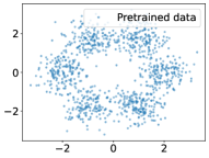
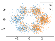
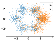
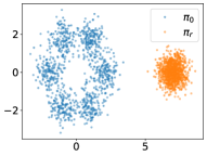
(a) Pretrained $\pi_{0}$	(b) Preferred $\pi_{r}$ ($\eta^{-1}=0.5$)	(c) Preferred $\pi_{r}$ ($\eta^{-1}=1.0$)	(d) Preferred $\pi_{r}$ ($\eta^{-1}=10$)

Figure 1: A two-dimensional illustrating example of human preference in generative modeling. We consider a scenario where the initial data distribution $\pi_{0}$, referred to as “pretrained”, is represented by a multi-modal Gaussian mixture, reflecting real-world data complexities. The “human preference” is expressed as a bias towards the right, as we set $r=[1,0]^{\top}a$. The KL penalty is critical in maintaining the desired behavior of $\pi_{r}$. By varying the values of $\eta$, we demonstrate the impact of KL regularization in (b)-(d). As $\eta$ approaches zero, $\pi_{r}$ increasingly focuses on maximizing rewards, often at the expense of the pretrained data’s structure, leading to a Gibbs distribution that potentially diverges infinitely.

In current RLHF theory, the agent’s objective is to maximize an observed reward function, with the optimal policy typically being deterministic and reward-greedy (Agarwal et al., 2019). However, in practical RLHF applications, merely maximizing the reward function is often insufficient and probably results in overfitting, as the generative model must simultaneously ensure both diversity and high fidelity in its outputs. A deterministic maximizer of the reward tends to compromise on these aspects significantly. For example, the maximizer of the “safety reward” tends to avoid providing answers all the time, which contradicts the LLM’s training objective. The situation worsens due to bias and approximation errors in reward modeling, leading to the critical problem of reward hacking, where the model often repeats superfluous, pleasing yet irrelevant words to appease the reward model (Michaud et al., 2020; Tien et al., 2022; Casper et al., 2023). Thus, it is important to model diversity and high fidelity in the theoretical framework beyond the reward. Notably, the most widely used mathematical objective function for this goal can be regarded as a reverse-KL regularized contextual bandit problem (Ziegler et al., 2019; Wu et al., 2021a; Ouyang et al., 2022; Rafailov et al., 2023; Liu et al., 2023a). The KL regularized contextual bandit additionally imposes a constraint that the optimal policy cannot move too far away from the original policy (i.e. the starting checkpoint of the LLM). A major difference between this objective function from traditional contextual bandit (Langford & Zhang, 2007) is that the optimal policy is stochastic, which is closer to the practical generative models. See an intuitive illustration why such a target is appealing in Figure 1. Despite numerous proposed procedures for this formulation, a rigorous theoretical analysis remains open. This paper provides a theoretical analysis of the regularized contextual bandit problem in both offline and online settings, aiming to inform and motivate practical algorithmic designs. Our contributions are summarized as follows:

• We formally formulate the RLHF process as a reverse-KL regularized contextual bandit problem in RLHF theory, which more accurately reflects real-world alignment practices (Ouyang et al., 2022; Bai et al., 2022a; Rafailov et al., 2023) compared to existing theoretical frameworks. Meanwhile, we deliver a comprehensive theoretical analysis in offline, online, and hybrid settings for the formulated framework, where the three settings are complementary to each other and hold their own values in practical applications;

• We introduce algorithms designed to address this formulated problem, which incorporate new uncertainty estimation or version space construction, and different non-symmetric exploration structures to handle the introduced KL penalty, as well as the challenges of preference learning;

• Moving towards practical applications, we demonstrate that the proposed algorithms can be practically implemented and empirically outperform existing strong baselines like DPO (Rafailov et al., 2023) and RSO (Liu et al., 2023a) in real-world LLM experiments.

1.1 Related Work

There is a rich literature in RLHF and we refer the interested readers to the survey papers like Casper et al. (2023) for a more comprehensive review. We focus on the papers that are most related to our work here.

RLHF has attracted considerable attention in the past few years, especially after its tremendous success in ChatGPT (OpenAI, 2023). We refer interested readers to Wirth et al. (2017); Casper et al. (2023) for a detailed survey but focus on the most related works here. The standard RLHF was popularized by Christiano et al. (2017), which served to direct the attention of the RL community to the preference-based feedback. The most popular and standard RLHF framework is outlined in the InstructGPT paper (Ouyang et al., 2022), Claude (Bai et al., 2022a) and the LLaMA2 report (Touvron et al., 2023) in detail, which typically consists of three steps starting from the pretrained model: supervised finetuning, reward modeling, and reward optimization. The effectiveness of this framework has been showcased by many recent generative models, like ChatGPT (OpenAI, 2023), Bard (Google, 2023), Claude (Anthropic, 2023), and LLaMA2 (Touvron et al., 2023). However, it is also noteworthy to indicate that the RLHF process often leads to degeneration in the performance of generation, commonly referred to as the “alignment tax” in the literature (Askell et al., 2021). This is usually because of the imperfection of the reward model and the model can make use of these imperfections to chase for a high reward. This phenomenon is referred to as the reward hacking (Michaud et al., 2020; Tien et al., 2022). It is also possible to apply RLHF to general generative models, like the diffusion model (Hao et al., 2022; Wu et al., 2023; Lee et al., 2023; Dong et al., 2023). In this work, we use the terminology and analysis of LLMs for better illustration, and defer the study of general generative models to future work.

RLHF algorithms. Proximal Policy Optimization (PPO) (Schulman et al., 2017) is the most well-known algorithm in LLM alignment literature. However, its instability, inefficiency, and sensitivity to hyperparameters (Choshen et al., 2019) and code-level optimizations (Engstrom et al., 2020) present significant challenges in tuning for optimal performance and its tremendous success in Chat-GPT4 (OpenAI, 2023) has not been widely reproduced so far. Additionally, it often necessitates incorporating an extra reward model, a value network (known as a critic), and a reference model, potentially as large as the aligned LLM (Ouyang et al., 2022; Touvron et al., 2023). This imposes a significant demand on GPU memory resources. Thus, researchers have attempted to design alternative approaches for LLM alignment to resolve the aforementioned issues. Dong et al. (2023); Yuan et al. (2023); Touvron et al. (2023); Gulcehre et al. (2023) propose reward ranked finetuning (RAFT) (also known as the iterative finetuning, rejection sampling finetuning) by iteratively learning from the best-of-n policy (Nakano et al., 2021) to maximize the reward, which is a stable baseline with minimal hyper-parameter configuration and was applied to the alignment of LLaMA2 project. There is also a line of work focusing on deriving an algorithm from the KL-regularized formulation (Rafailov et al., 2023; Zhu et al., 2023b; Wang et al., 2023a; Liu et al., 2023a; Li et al., 2023a). Among them, Direct Preference Optimization (DPO) (Rafailov et al., 2023) has emerged as an attractive alternative approach to PPO with notable stability and competitive performance. The innovative idea of DPO is to train the LLMs directly as a reward model based on the offline preference dataset and bypassing the reward modeling. Similar to DPO, there are also other works aiming to optimize the LLMs directly from the preference data, including (Zhao et al., 2023; Azar et al., 2023), and has sparked considerable debate on whether reward modeling, as well as RL, is necessary for alignment. However, while these algorithms are partly inspired by mathematical principles and intuitions, a comprehensive theoretical analysis remains open.

Theoretical study of RLHF. The theoretical understanding of RLHF can be traced back to research on dueling bandits (e.g., Yue et al., 2012; Saha, 2021; Bengs et al., 2021), a simplified setting within the RLHF framework. Recently, many works have focused on the more challenging RLHF problem (also known as the preference-based RL). Xu et al. (2020); Novoseller et al. (2020); Pacchiano et al. (2021) delve into the study of tabular online RLHF, where the state space is finite and small. Moving beyond the tabular setting, Chen et al. (2022) provides the first results for online RLHF with general function approximation, capturing real-world problems with large state spaces. Wang et al. (2023c) presents a reduction-based framework, which can transform some sample-efficient algorithms for standard reward-based RL to efficient algorithms for online RLHF. Further advancements in algorithm designs are introduced by Zhan et al. (2023b); Wu & Sun (2023), encompassing the development of reward-free learning type algorithms and posterior sampling-based algorithms tailored for online RLHF. Initiating exploration into offline RLHF, Zhu et al. (2023a) presents a pessimistic algorithm that is provably efficient for offline RLHF. Additionally, Zhan et al. (2023a) and Li et al. (2023b) extend these investigations into the broader scope of general function approximation settings within offline RLHF. In comparison to these existing studies, our work introduces a new theoretical formulation and goal for RLHF, as well as novel problem settings, such as hybrid RLHF. The new mathematical formulation allows our framework to align more closely with recent advancements in LLMs, and we discuss the connections between our theoretical findings and practical algorithmic designs in Section 5.

Finally, concurrent to this work, Hoang Tran (2024) and Yuan et al. (2024) also consider variants of iterative DPO. We comment on the similarities and differences between our work and theirs as follows. Hoang Tran (2024) focuses on the batch online setting, which will be thoroughly developed in Theorem B.2 (as well as Algorithm 5) in this paper. We notice that Theorem B.2 essentially states that, for exploitation, we should choose the policies (LLMs) around $\pi_{r^{t}}$, i.e., the Gibbs distribution induced by $r^{t}$ (see Section 2 for formal definitions), and for exploration, we should increase the diversity by making two policies more different. In comparison, Hoang Tran (2024) sets the two policies as the best-of-4 policy and worst-of-4 policy induced by the a preference model PairRM-0.4B (Jiang et al., 2023) and $\pi_{r^{t}}$, which may be viewed as a reasonable practical approximation of the exploration-exploitation trade-off presented in Theorem B.2. Meanwhile, the resulting model from Hoang Tran (2024) achieves state-of-the-art (SOTA) performance in the AlpacaEval leaderboard even though the preference oracle is of only 0.4B parameters. This may also partially verify that the sample complexity of alignment depends on the complexity of reward/preference model space, which can be much smaller than that of the generator (also see Theorem B.2 for details). To summarize, the two works are complementary to each other, as Hoang Tran (2024) presents an exciting recipe to illustrate the effectiveness of batch-online iterative DPO, while our work focuses more on the theoretical side. Yuan et al. (2024) also proposes a variant of iterative DPO in the batch online setting but in a self-rewarding manner. The main difference between Yuan et al. (2024) and our work (as well as Hoang Tran (2024)) is that instead of optimizing against an external preference oracle, they adopt a clever idea by using the LLM itself as the reward model to provide preference signal, hence the name “self-rewarding”. We also remark that in addition to the practical algorithmic designs, our work also serves to establish the mathematical foundation of the RLHF, in offline, online, and hybrid settings.

2 Formulation of RLHF

In this section, we present the mathematical framework for the RLHF process, inspired by the standard LLM alignment workflow (Ouyang et al., 2022; Touvron et al., 2023).

Specifically, the LLM can take a prompt, denoted by $x\in\mathcal{X}$, and produce a response, denoted by $a=[w_{1},w_{2},\ldots]$, where $w_{i}$ is the $i$-th token generated by the model. Accordingly, we can take $\mathcal{X}$ as the state space of the contextual bandit and the $\mathcal{A}$ as the action space. Following Ouyang et al. (2022); Zhu et al. (2023a); Rafailov et al. (2023); Liu et al. (2023a), we assume that there exists a ground-truth reward function $r^{*}(x,a):\mathcal{X}\times\mathcal{A}\to[0,1]$ and the preference satisfies the Bradley-Terry model (Bradley & Terry, 1952):

$$\mathbb{P}(a^{1}\succ a^{2}|x,a^{1},a^{2}) =\frac{\exp(r^{*}(x,a^{1}))}{\exp(r^{*}(x,a^{1}))+\exp(r^{*}(x,a^{2}))}$$ (1)

$$=\sigma\big{(}r^{*}(x,a^{1})-r^{*}(x,a^{2})\big{)},$$

where $a^{1}\succ a^{2}$ means that $a^{1}$ is preferred to $a^{2}$, and $\sigma(z)=1/(1+\exp(-z))$ is the sigmoid function. We denote an LLM by a policy $\pi$ that maps $x$ to a distribution over $\mathcal{A}$.

In a typical LLM training pipeline, the tuning process begins with a pretrained LLM, which is subsequently fine-tuned using specialized and instructional data, yielding an initial LLM policy denoted as $\pi_{0}$. We will then align the LLM on RLHF data (prompt set), which we assume is taken from a distribution $x\sim d_{0}$. For preference learning, the way to gather information from the environment is to compare two different actions under the same state. Considering this, we assume that the agent can perform a pair of actions, aligning with precedents in existing literature (Novoseller et al., 2020; Pacchiano et al., 2021). In applications, we want the resulting LLM $\pi$ to be close to $\pi_{0}$, and our goal is to find a policy $\pi$ from some policy class $\Pi$ to maximize

$$J(\pi) =\mathbb{E}_{x\sim d_{0}}\mathbb{E}_{a\sim\pi(\cdot|x)}\left[r^{*}(x,a)+\eta\log\frac{\pi_{0}(a|x)}{\pi(a|x)}\right]$$ (2)

$$=\mathbb{E}_{x\sim d_{0}}\left[\mathbb{E}_{a\sim\pi(\cdot|x)}[r^{*}(x,a)]-\eta D_{\mathrm{KL}}(\pi(\cdot|x)\|\pi_{0}(\cdot|x))\right],$$

where $\eta>0$ is the KL penalty coefficient. This formulation is widely studied in practice (Ziegler et al., 2019; Wu et al., 2021a; Ouyang et al., 2022; Rafailov et al., 2023; Liu et al., 2023a), and our paper aims to study its theoretical property.

Usually, we have a function class $\mathcal{F}$ for approximating the ground truth $r^{*}$. Following Pacchiano et al. (2021); Kong & Yang (2022); Zhu et al. (2023a), we make the following assumption for a clear presentation because it suffices to illustrate our ideas and the algorithmic design in this paper can also apply to the general case. The analysis also readily generalizes to general function class using standard complexity measures in RL theory literature (Russo & Van Roy, 2013; Gentile et al., 2022), which essentially state that there are some low-rank structures in reward model.

Assumption 2.1.

Assume that the reward function is parameterized by $r_{\theta}(x,a)=\left\langle\theta,\phi(x,a)\right\rangle$ for feature extractor $\phi:\mathcal{X}\times\mathcal{A}\to\mathbb{R}^{d}$. We also assume that $r^{*}(x,a)=\left\langle\theta^{*},\phi(x,a)\right\rangle$ for some $\theta^{*}\in\mathbb{R}^{d}$. For regularization, we assume that $\|\phi(x,a)\|\leq 1$ for all possible $(x,a)\in\mathcal{X}\times\mathcal{A}$ and $\|\theta\|\leq B$.

Notation. We use $\|z\|_{\Sigma}$ to denote the induced norm $\sqrt{z^{\top}\Sigma z}$ for some positive-definite matrix. We also define $\phi(x,\pi):=\mathbb{E}_{a\sim\pi(\cdot|x)}\phi(x,a)$ to simplify the presentation. We use $\widetilde{O}$ when we omit the logarithmic factors. A notation table is provided in Table 2 to improve the readability of this paper.

2.1 Maximum Likelihood Estimation and Policy Improvement Oracle

The most common way of reward modeling is Maximum Likelihood Estimation (MLE) (e.g., Ouyang et al., 2022; Bai et al., 2022a; Touvron et al., 2023).

Maximum Likelihood Estimation. A preference dataset $\mathcal{D}$ consists of numerous tuples, such as $(x,a^{1},a^{2},y)$, where $y$ is the preference signal. Specifically, $y=1$ means a preference for $a^{1}\succ a^{2}$, while $y=0$ indicates $a^{1}\prec a^{2}$. Given a dataset $\mathcal{D}=\{(x,a^{1},a^{2},y)\}$, we can write the log-likelihood function of the BT models as follows:

$$\ell_{\mathcal{D}}(\theta) =\sum_{(x,a^{1},a^{2},y)\in\mathcal{D}}\Big{[}y\log\Big{(}\sigma\big{(}r_{\theta}(x,a^{1})-r_{\theta}(x,a^{2})\big{)}\Big{)}$$ (3)

$$\qquad+(1-y)\log\Big{(}\sigma\big{(}r_{\theta}(x,a^{2})-r_{\theta}(x,a^{1})\big{)}\Big{)}\Big{]}.$$

The MLE is $\theta_{\mathrm{MLE}}=\mathop{\mathrm{argmax}}_{\theta\in\Theta(B)}\ell_{\mathcal{D}}(\theta)$ with $\Theta(B)=\{\theta\in\mathbb{R}^{d}:\|\theta\|\leq B\}$. In practice, the MLE is also conducted with the LLMs (Touvron et al., 2023) on the preference dataset. We define the following information-theoretical policy improvement oracle, and defer a discussion on its practical implementations in Section 5.

Definition 2.2 (Policy Improvement Oracle).

For reward function $r:\mathcal{X}\times\mathcal{A}\to\mathbb{R}$ and a reference policy $\pi_{0}$, for all $x\in\mathcal{X}$, we can compute the Gibbs policy (Lemma G.6):

$$\pi_{r}(\cdot|x) :=\mathop{\mathrm{argmax}}_{\pi\in\Pi}\mathbb{E}_{a\sim\pi(\cdot|x)}\Big{[}r(x,a)+\eta\log\frac{\pi_{0}(a|x)}{\pi(a|x)}\Big{]}$$

$$\propto\pi_{0}(\cdot|x)\cdot\exp\big{(}\frac{1}{\eta}r(x,\cdot)\big{)}.$$

Accordingly, we take the policy class as $\Pi:=\big{\{}\pi(\cdot|x)\propto\pi_{0}(\cdot|x)\cdot\exp\big{(}\frac{1}{\eta}\left\langle\theta,\phi(x,\cdot)\right\rangle\big{)}:\theta\in\Theta(B)\big{\}}.$ The goal is to design a sample-efficient algorithm, which finds a policy $\hat{\pi}\in\Pi$ so that the suboptimality $J(\pi)-J(\hat{\pi})<\epsilon$ with the number of samples polynomial in accuracy parameter $1/\epsilon$, feature dimension $d$, and other problem-dependent parameters, where $\pi$ is a comparator policy (e.g. $\pi^{*}$).

2.2 Preliminary

In this section, we present some useful technical tools and lemmas for subsequent analysis.

Value decomposition. We have the following lemma to decompose the value difference.

Lemma 2.3.

Given a comparator policy $\pi$, we can decompose the suboptimality of $\hat{\pi}$ as follows:

$$J(\pi)-J(\hat{\pi})=\mathbb{E}_{x\sim d_{0}}\Big{[}{\mathbb{E}_{\pi}[r^{*}(x,a)-\hat{r}(x,a)]}$$

$$\qquad+{\mathbb{E}_{\hat{\pi}}[\hat{r}(x,a)-r^{*}(x,a)]}+\mathbb{E}_{\pi}[\hat{r}(x,a)]-\mathbb{E}_{\hat{\pi}}[\hat{r}(x,a)]$$

$$\qquad+\eta D_{\mathrm{KL}}(\hat{\pi}(\cdot|x)\|\pi_{0}(\cdot|x))-\eta D_{\mathrm{KL}}(\pi(\cdot|x)\|\pi_{0}(\cdot|x))\Big{]},$$

where $\hat{r}:\mathcal{X}\times\mathcal{A}\to\mathbb{R}$ is arbitrary.

Proof.

The equality can be verified directly by the definition of $J(\cdot)$ in Equation (2) and basic algebra. ∎

Policy improvement error. In standard RL setting, $\hat{\pi}$ is typically taken as a greedy policy of $\hat{r}$, leading to

$$\mathbb{E}_{\pi}[\hat{r}(x,a)]-\mathbb{E}_{\hat{\pi}}[\hat{r}(x,a)]\leq 0.$$

In the KL-constrained case, since the policy cannot be greedy or deterministic, we need to additionally handle the policy improvement error. The following lemma provides such an estimation when our policy is obtained by calling the Oracle 2.2 with $\hat{r}$.

Lemma 2.4 (Policy optimization error).

Suppose that $\pi,\hat{\pi}\in\Pi$ so that $\pi_{0},\pi,\hat{\pi}$ have the same support. If $\hat{\pi}$ is induced by calling Oracle 2.2 with $\hat{r}$, it holds that

$$\mathbb{E}_{x\sim d_{0}}\Big{[}\mathbb{E}_{\pi}[\hat{r}(x,a)]-\mathbb{E}_{\hat{\pi}}[\hat{r}(x,a)]+\eta D_{\mathrm{KL}}(\hat{\pi}\|\pi_{0})-\eta D_{\mathrm{KL}}(\pi\|\pi_{0})\Big{]}$$

$$=-\eta\mathbb{E}_{x\sim d_{0}}D_{\mathrm{KL}}(\pi\|\hat{\pi}).$$

Here $D_{\mathrm{KL}}(\pi\|\pi_{0})$ is short for $D_{\mathrm{KL}}(\pi(\cdot|x)\|\pi_{0}(\cdot|x))$.

We will provide the proof of the lemma in Appendix F. The analysis techniques are most similar to the policy gradient literature since they also consider the soft-max policies (Agarwal et al., 2021; Cai et al., 2020; Zanette et al., 2021b; Zhong & Zhang, 2023). The main difference is that in their iterative choices of policy, for choosing $\pi_{t}$, the reference policy they use is the policy of the last round, i.e., $\pi_{t-1}$, while we always use the SFT-model $\pi_{0}$ as our reference. We note that their algorithms essentially still use the non-KL-regularized reward as the target because though we prevent the policy from moving too far away in each individual step, the cumulative updates makes the reward estimations dominating in the final policy.

Covariance matrix. Given a preference dataset $\mathcal{D}$, a fixed $\lambda>0$, we denote $\Sigma_{\mathcal{D}}$ as the covariance matrix estimation:

$$\lambda I+\sum_{(x,a^{1},a^{2})\in\mathcal{D}}\big{(}\phi(x,a^{1})-\phi(x,a^{2})\big{)}\big{(}\phi(x,a^{1})-\phi(x,a^{2})\big{)}^{\top}.$$

Both the algorithmic design and analysis will be centered on the covariance matrix. For the readers that are not familiar with the eluder-type techniques (or elliptical potential lemma in this case), we provide a brief introduction to the high-level intuition in Appendix A.1.

3 Offline learning

In the offline setting, we aim to learn a good policy from a pre-collected dataset without further interactions with the human. We suppose that we are given an offline preference dataset: $\mathcal{D}_{\mathrm{off}}=\{(x_{i},a_{i}^{1},a_{i}^{2},y_{i})\}_{i=1}^{n_{\mathrm{off}}}.$ We denote $\Sigma_{\mathrm{off}}:=\Sigma_{\mathcal{D}_{\mathrm{off}}}$ for offline setting. To motivate the algorithmic design, we recall Lemma 2.3 and Lemma 2.4 to obtain that

$$J(\pi^{*})-J(\hat{\pi})$$

$$=\mathbb{E}_{x\sim d_{0}}\Big{[}{\mathbb{E}_{\pi}[r^{*}(x,a)-\hat{r}(x,a)]}+{\mathbb{E}_{\hat{\pi}}[\hat{r}(x,a)-r^{*}(x,a)]}$$

$$\qquad-\eta\cdot\mathbb{E}_{x\sim d_{0}}\big{[}D_{\mathrm{KL}}(\pi^{*}(\cdot|x)\|\hat{\pi}(\cdot|x))\Big{]},$$

where $\hat{\pi}$ is induced by calling the Oracle 2.2 with $\hat{r}$. As suggested in the offline learning literature (Jin et al., 2021b; Rashidinejad et al., 2021), the first term can typically controlled by the property of $\mathcal{D}_{\mathrm{off}}$, while the second term is far more challenging to control because both the $\hat{\pi}$ and $\hat{r}$ are estimated from $\mathcal{D}_{\mathrm{off}}$, and hence spuriously correlate with each other. The standard methods to handle such a spurious correlation is to introduce pessimism in the algorithmic designs, which means that we adopt an estimator that is a lower bound of the true value with high probability. Specifically, instead of taking the MLE estimator directly, we penalize the reward estimation by an uncertainty estimator $\hat{r}(x,a)=r_{\mathrm{MLE}}(x,a)-\beta\cdot\Gamma(x,a,\nu,\mathcal{D}_{\mathrm{off}})$ so that $\hat{r}(x,a)-r^{*}(x,a)\leq 0$ for all $(x,a)\in\mathcal{X}\times\mathcal{A}$ and the spuriously correlated term can be eliminated. The construction of the uncertainty bonus is a standard application of concentration inequality, and we defer the details to Appendix C.

In addition to adopting a pessimistic reward estimation, we may also use a modified target that is biased toward pessimism by penalizing the uncertainty as in Equation (4). Here we do not maintain a confidence set but use a modified target that is biased toward pessimism, similar to Xie et al. (2021a); Zhang (2022), which may be easier to approximate in practice (Liu et al., 2023b). Moreover, to handle the additional trade-off between the reward and the KL term, we also incorporate the KL divergence into the policy computation.

The full algorithm is presented in Algorithm 1 and is referred to as the offline Gibbs Sampling from Human Feedback (GSHF) because the output policy is the Gibbs distribution with some reward.

Algorithm 1 Offline GSHF

1:  Input: $\mathcal{D}_{\mathrm{off}}$, $\lambda>0$, $\beta>0$, reference vector $\nu$, and prompt distribution $d_{0}$.

2:  Compute $\theta_{\mathrm{MLE}}$ based on $\mathcal{D}_{\mathrm{off}}$ by maximizing the likelihood given in Equation (3)

3:  Option I: Output $\hat{\pi}$ by constructing expected uncertainty estimator $\Gamma^{e}(\pi,\nu,\mathcal{D}_{\mathrm{off}})$ and solving

$$\hat{\pi} =\mathop{\mathrm{argmax}}_{\pi\in\Pi}\Big{[}\mathbb{E}_{x\sim d_{0},a\sim\pi(\cdot|x)}[r_{\mathrm{MLE}}(x,a)]-\beta\cdot\Gamma^{e}(\pi,\nu,\mathcal{D}_{\mathrm{off}})$$ (4)

$$\qquad-\eta\cdot\mathbb{E}_{x\sim d_{0}}[D_{\mathrm{KL}}(\pi(\cdot|x)\|\pi_{0}(\cdot|x))]\Big{]}.$$

4:  Option II: Output $\hat{\pi}$ by constructing uncertainty estimator $\Gamma(x,a,\nu,\mathcal{D}_{\mathrm{off}})$ and calling Oracle 2.2 with $\hat{r}(x,a)=r_{\mathrm{MLE}}(x,a)-\beta\cdot\Gamma(x,a,\nu,\mathcal{D}_{\mathrm{off}})$.

We also have the theoretical guarantee in Theorem 3.1.

Theorem 3.1.

Under Assumption 2.1, if we set $\beta:=O\big{(}\sqrt{\frac{d+\log(1/\delta)}{\gamma^{2}}+\lambda B^{2}}\big{)}$, for any $\lambda>0$ and comparator policy $\pi\in\Pi$, with probability at least $1-\delta$, the output policy of Algorithm 1 with Option I and $\Gamma^{e}(\pi,\nu,\mathcal{D}_{\mathrm{off}})=\|\mathbb{E}_{x\sim d_{0}}[\phi(x,\pi)-\nu]\|_{\Sigma_{\mathrm{off}}^{-1}}$ satisfies

$$J(\pi)-J(\hat{\pi})\leq 2\beta\cdot\|\mathbb{E}_{x\sim d_{0}}[\phi(x,\pi)]-\nu\|_{\Sigma_{\mathrm{off}}^{-1}},$$

and the output policy of Algorithm 1 with Option II and $\Gamma(x,a,\nu,\mathcal{D}_{\mathrm{off}})=\|\phi(x,a)-\nu\|_{\Sigma_{\mathrm{off}}^{-1}}$ satisfies

$$J(\pi)-J(\hat{\pi}) \leq 2\beta\cdot\mathbb{E}_{x\sim d_{0},a\sim\pi(\cdot|x)}\|\phi(x,a)-\nu\|_{\Sigma_{\mathrm{off}}^{-1}}$$

$$\qquad-\eta\cdot\mathbb{E}_{x\sim d_{0}}\big{[}D_{\mathrm{KL}}(\pi(\cdot|x)\|\hat{\pi}(\cdot|x))\big{]}.$$

We can combine the guarantee with dataset property, usually referred to as the coverage on the comparator policy $\pi$ (Jin et al., 2021b; Xie et al., 2021a), to obtain the concrete bound. See Proposition D.1 for an concrete example. The proof of the theorem is rather standard in offline learning based on the principle of pessimism but with a different analysis to handle the KL and the stochastic policy. We defer the proof of the theorem to Appendix C.

The reference vector $\nu$ in Algorithm 1 is typically set as $\mathbb{E}_{x\sim d_{0}}[\phi(x,\pi_{\mathrm{ref}})]$ for some available $\pi_{\mathrm{ref}}$. As showcased by Zhu et al. (2023a), the subtracted reference vector can serve as a pre-conditioner for a better suboptimality bound. For instance, one typically choice is $\pi_{\mathrm{ref}}=\pi_{0}$ so that $\pi_{0}$ achieves a reward of zero (Ouyang et al., 2022; Gao et al., 2023; Dong et al., 2023).

In comparison, the Option I achieves a sharper bound in the uncertainty bonus because the expectation is inside the norm and by Jensen’s inequality (Lemma G.1) we know that

$$\|\mathbb{E}_{x\sim d_{0}}[\phi(x,\pi)]-\nu\|_{\Sigma_{\mathrm{off}}^{-1}}\leq\mathbb{E}_{x\sim d_{0},a\sim\pi(\cdot|x)}\|\phi(x,a)-\nu\|_{\Sigma_{\mathrm{off}}^{-1}}.$$

Moreover, Option I has a desirable robust improvement property. If we take $\nu=\mathbb{E}_{x\sim d_{0}}[\phi(x,\pi_{\mathrm{ref}})]$, the resulting policy will be better than $\pi_{\mathrm{ref}}$, regardless of the coverage of the $\mathcal{D}_{\mathrm{off}}$ according to Theorem 3.1, which is similar to the original offline RL literature for a robust policy improvement (Bhardwaj et al., 2023). We will also see that the use of a reference policy $\pi_{\mathrm{ref}}$ can also simplify the algorithmic design in subsequent Section 4. However, the main advantage of Option II is that the Oracle 2.2 can be well approximated by some empirical counterpart. We defer a detailed discussion to Section 5.

4 Hybrid Learning with Batch Exploration

Beyond the offline learning, it is also common to query human feedback during the training process. For instance, Bai et al. (2022a); Touvron et al. (2023) typically iterate the RLHF process on a weekly cadence, where the fresh RLHF models are deployed to interact with crowdworkers and to collect new human preference data.

While it is possible to learn from scratch, in many cases, we tend to start with the offline open-source datasets (Touvron et al., 2023; Bai et al., 2023). For instance, in LLaMA2 (Touvron et al., 2023), the authors start with 1500K open-source comparison pairs $\mathcal{D}_{\mathrm{off}}$ and keep $\mathcal{D}_{\mathrm{off}}$ in the data mixture for the entire RLHF process. Motivated by the practical applications, we formulate the process as a batch hybrid framework in this section. It is shown that such a batch online framework can significantly improve the aligned LLMs as evaluated by the humans (Bai et al., 2022a; Touvron et al., 2023). For completeness, we also develop the pure online setting in Appendix B. Mathematically, consider the batch hybrid setting of $T$ batches with a fixed batch size $m$. The agent starts with the offline dataset $\mathcal{D}_{\mathrm{off}}$. At the beginning of each batch $t\in[T]$, An agent updates the policies $\pi_{t}^{1}$ and $\pi_{t}^{2}$. Then, the agent collects $m$ tuples $(x_{t,i},a_{t,i}^{1},a_{t,i}^{2})_{i=1}^{m}$ using the two policies, and the human preference signals $y_{t,i}\in\{0,1\}$ are yielded according to the underlying BT model.

Non-symmetric algorithmic structure. The main technical challenge here is to decide the behavior policy pairs $(\pi_{t}^{1},\pi_{t}^{2})$. Our first idea is to adopt a non-symmetric structure in choosing $\pi_{t}^{1}$ and $\pi_{t}^{2}$. Specifically, we refer the $\pi_{t}^{1}$ as the main agent, which aims to learn a good policy so that the suboptimality gap $J(\pi^{*})-J(\pi_{t}^{1})$ is small. In contrast, the second agent, referred to as the enhancer, seeks to enhance the learning of the main agent by choosing appropriate $\pi_{t}^{2}$. The main advantage of such a non-symmetric structure is that we have a lot of freedoms to choose $\pi_{t}^{2}$ because we do not worry about the sub-optimality incurred by it. Using $\pi_{t}^{2}$ as an intermediate agent in Lemma 2.3, we have

$$J(\pi^{*})-J(\pi_{t}^{1}) \leq\mathbb{E}_{x_{t}\sim d_{0}}\Big{[}\left\langle\theta^{*}-\theta^{t},\phi(x_{t},\pi^{*})-\phi(x_{t},\pi_{t}^{2})\right\rangle\Big{]}$$ (5)

$$\quad+\mathbb{E}_{x_{t}\sim d_{0}}\Big{[}\left\langle\theta^{t}-\theta^{*},\phi(x_{t},\pi^{1}_{t})-\phi(x_{t},\pi_{t}^{2})\right\rangle\Big{]},$$

where we omit the KL error to simplify the discussion. The idea is most related to the hybrid RL theory to use $\mathcal{D}_{\mathrm{off}}$ to handle the term related to $\pi^{*}$ (Song et al., 2022). However, for preference-based learning, one major difference is that the uncertainty is evaluated on the feature difference instead of a single state-action pair, which calls for an appropriate choice of $\pi_{t}^{2}$ to balance the sub-optimality sources. To this end, we introduce the reference policy $\pi_{\mathrm{ref}}$, which satisfies the following two conditions. First, the $\pi_{\mathrm{ref}}$ may serve as the pre-conditioner for the offline coverage similar to Theorem 3.1 to control the first term related to $\pi^{*}$.

Assumption 4.1 (Partial Coverage of Offline Data).

For the linear model, there exists a reference policy $\pi_{\mathrm{ref}}$, a ratio coefficient $\alpha(mT,\mathcal{D}_{\mathrm{off}})\in(0,1)$ and a coverage constant $C_{\mathrm{cov}}>0$ such that

$$(mT)^{1-\alpha(mT,\mathcal{D}_{\mathrm{off}})}\|\mathbb{E}_{x\sim d_{0}}[\phi(x,\pi^{*})-\phi(x,\pi_{\mathrm{ref}})]\|_{(\Sigma_{\mathrm{off}})^{-1}}\leq C_{\mathrm{cov}}.$$

We remark that Assumption 4.1 implicitly assume that $n_{\mathrm{off}}$ is comparable to the total number of online samples $mT$ so that the influence of $\mathcal{D}_{\mathrm{off}}$ will not be dominated by the online data. To provide a more detailed understanding and connection to existing literature, we offer a more nuanced characterization of $\alpha(mT,\mathcal{D}_{\mathrm{off}})$ under standard partial coverage conditions in Appendix D.1. In particular, when $mT\approx n_{\mathrm{off}}$, we show that $\alpha(mT,\mathcal{D}_{\mathrm{off}})\approx 1/2$. It is worth emphasizing that this scenario appears to be realistic for LLMs. For example, in the LLaMA2 project (Touvron et al., 2023), we observe $n_{\mathrm{off}}=1500K$ and $mT=1400K$.

Moreover, to control the second term of Equation (5), we typically invoke the elliptical potential lemma (Lemma G.4). This requires that the reference policy should be available for collecting new data so the analysis target ($\pi_{t}^{1}$ and $\pi_{\mathrm{ref}}$) and the policies used to collect data are identical. We present the complete algorithm in Algorithm 2 and the theoretical guarantee as follows.

Algorithm 2 Hybrid GSHF

1:  Input: $m,\Pi,\mathcal{D}_{\mathrm{off}},\mathcal{D}^{0}=\emptyset$, and $\pi_{\mathrm{ref}}$.

2:  for $t=1,2,\cdots,T$ do

3:     Compute the MLE $r^{t}$ based on $\mathcal{D}_{\mathrm{off}}$ and $\mathcal{D}^{1:t-1}$ with Equation (3).

4:     Compute the policy $\pi_{t}$ by calling the oracle in Assumption 2.2 with $r^{t}$;

5:     Observe $x_{t,i}\sim d_{0}$, sample $a_{t,i}^{1}\sim\pi_{t}$ and $a_{t,i}^{2}\sim\pi_{\mathrm{ref}}$, receive human feedback for all $i\in[m]$, and collect them as $\mathcal{D}^{t}$.

6:  end for

7:  Output: the best model in $\pi_{1:T}$ by a validation set.

Theorem 4.2.

For any $\epsilon>0$, under Assumption 2.1 and  4.1, for Algorithm 2 with $T=\min\{n\in\mathbb{N}^{+}:n\geq d\log(n)\}$ and $\beta=O\big{(}\sqrt{\frac{d\log(T/\delta)}{\gamma^{2}}}\big{)}$, with probability at least $1-3\delta$, there exists a $t_{0}\in[T]$ such that

$$J(\pi^{*})-J(\pi_{t_{0}}) \lesssim\sqrt{\frac{d^{2}}{\gamma^{2}m}}+\beta(mT)^{\alpha(mT,\mathcal{D}_{\mathrm{off}})-1}C_{\mathrm{cov}}$$

$$\qquad-\eta\mathbb{E}_{x_{t_{0}}\sim d_{0}}\big{[}D_{\mathrm{KL}}(\pi^{*}(\cdot|x_{t_{0}})\|\pi_{t_{0}}(\cdot|x_{t_{0}}))\big{]}.$$

The proof is deferred to Appendix D.3.

The advantage of reward modeling. Theorem 4.2 and Theorem B.2 (for the online setting) reveal a key characteristic of reward modeling: the sample complexity is dependent on the complexity of the reward model rather than the generative models. For simple reward functions, such as sentiment or politeness evaluation, the required function class is substantially smaller compared to the generative model. This is corroborated by evidence showing that even compact models like BERT (Devlin et al., 2018) can yield accurate reward assessments. Besides, the reward function can also be recognized as a density ratio estimator, similar to the discriminator in Generative Adversarial Models (Goodfellow et al., 2014). The density ratio estimator can be applied to generative models without explicit likelihood (GAN, Energy-based models). Johnson & Zhang (2019) suggest that the distribution induced by the density ratio estimator is more stable than optimizing the generative model. Meanwhile, the density ratio estimator approximates the functional gradient in probability space, iterative reward modeling provides a provable path towards the target distribution. This may illustrate the advantage of the most popular RLHF framework used by Ouyang et al. (2022); Bai et al. (2022a); Touvron et al. (2023), in contrast to the idea of bypassing reward modeling (Rafailov et al., 2023; Zhao et al., 2023; Azar et al., 2023) and training based only on the offline dataset. In summary, reward learning typically exhibits lower sample dependency and results in a more stable induced distribution compared to that learned directly through generative modeling. Iterative reward modeling approximates the functional gradient in probability space. Furthermore, it can be effectively applied to universal generative models, even those without explicit likelihood (Goodfellow et al., 2014; Grathwohl et al., 2019; Du & Mordatch, 2019).

5 Practical Implementations of GSHF

In this section, we discuss how to practically implement the information-theoretical Algorithm 1 and Algorithm 2.

5.1 Approximate Information-Theoretical Oracle by Existing RLHF Algorithms

The main challenge to apply the theoretical algorithm lies in the Oracle 2.2, which is computationally intractable due to the exponential action space. To design an implementable algorithm, it is critical to approximate $\pi_{r}$ effectively.

In practice, the policy is represented by a deep neural network. In this case, one common choice (Ziegler et al., 2019; Wu et al., 2021a; Ouyang et al., 2022; Bai et al., 2022a) is to use the standard deep RL algorithms like PPO to optimize the regularized reward:

$$\widetilde{r}(x,a)=r(x,a)-\eta\log\frac{\pi_{\theta}(a|x)}{\pi_{0}(a|x)}.$$

However, PPO is significantly less stable and sensitive to implementation as compared to SFT (Choshen et al., 2019; Engstrom et al., 2020). Recently, DPO (Rafailov et al., 2023) attracted significant attention due to its stability and easy implementation. Specifically, DPO chooses to train the LLM as a reward model, by optimizing the following loss:

$$\sum_{(x,a_{c},a_{r})\in\mathcal{D}_{\mathrm{off}}}-\Big{[}\log\sigma\Big{(}\eta\log\frac{\pi_{\theta}(a_{c}|x)}{\pi_{0}(a_{c}|x)}-\eta\log\frac{\pi_{\theta}(a_{r}|x)}{\pi_{0}(a_{r}|x)}\Big{)}\Big{]},$$ (6)

where $a_{c}$, $a_{r}$ is the chosen/rejected response. It is shown that the optimal policy for the DPO loss in Equation (6) is identical to the one for the RLHF objective $\pi_{r}$, with $r$ as the MLE of Equation (3). To summarize, to move toward a practical approach from the theoretical algorithms, we may just replace the Oracle 2.2 with the practical RLHF algorithms (both deep RL methods or non-RL methods). In view of the simplicity and effectiveness of DPO, we will mainly investigate the performance of the proposed GSHF framework with DPO.

5.2 Multi-step Rejection Sampling for Offline Learning

Algorithm 3 Offline GSHF (Practical Implementation)

1:  Input: Offline dataset $\mathcal{D}_{\mathrm{off}}$, KL regularization strength $\eta_{1}>\cdots>\eta_{N}=\eta$.

2:  Compute the reward estimator $\hat{r}(x,a)$ based on $\mathcal{D}_{\mathrm{off}}$.

3:  for $i=1,2,\cdots,N$ do

4:     Denote $\pi^{i}_{\hat{r}}(\cdot|x)\propto\pi_{0}(\cdot|x)\cdot\exp\Big{(}\frac{1}{\eta_{i}}\hat{r}(x,\cdot)\Big{)}$

5:     Sample from $\pi^{i}_{\hat{r}}$, where $\pi^{i}_{\hat{r}}$ is obtained by rejection sampling from $\pi_{i-1}$. Use $\hat{r}$ to label the paired samples. Wrap up the data as $\mathcal{D}^{i}$.

6:     Use DPO with $\mathcal{D}^{i}$ to train $\pi_{i}\approx\pi^{i}_{\hat{r}}$.

7:  end for

8:  Output: Set $\pi=\pi_{N}$

Recently, Liu et al. (2023a) found that the usage of offline datasets typically impedes the effectiveness of DPO-based algorithms. This negative impact is particularly pronounced when there is a disparity between the distribution of offline data and the target distribution. They emphasize the importance of sourcing offline training data from the target distribution. Consequently, they trained a reward model, denoted as $r$, and approximated samples from $\pi_{r}$ using rejection sampling. We provide a brief introduction to rejection sampling in Appendix A.2. In this case, they generate samples from the optimal policy of the underlying BT model associated with $r$ and get $\mathcal{D}_{\mathrm{gen}}=\{(x,a^{1},a^{2},y)\}$. The authors suggested that this is more suitable for DPO training and leads to better performance. The key basis of the success of RSO is that the rejection sampling can well approximate $\pi_{r}$.

However, in practice, the rejection rate can be so large that the sampling is not effective. Given a prompt-response pair $(x,a)$, the rejection rate is $1-\exp(-\eta^{-1}(R(x)-r(x,a)))$, where $R(x)$ is the largest possible reward over all $a\in\mathcal{A}$. For example, given $\eta>0$, if the samples drawn from $\pi_{0}(a|x)$ satisfies $\mathbb{E}_{a\sim\pi_{0}(a|x)}\exp(\eta^{-1}r(x,a))=\exp(-\eta^{-1}(r_{x}-R(x)))$, the expected acceptance rate becomes $\exp(-\frac{r_{x}}{\eta})$, where $r_{x}$ is the reward gap between average sample and the best sample given prompt $x$. Setting $r_{x}=1$ and $\eta=0.1$ yields a notably low acceptance rate of approximately $0.00004$. Essentially, the majority of samples are rejected, necessitating a substantial number of sampled candidates to produce a single accepted comparison pair. In the practical implementation of RSO (Liu et al., 2023a), we typically fix the total budget of candidate responses and the number of samples to be accepted. In this case, due to the low sampling efficiency, the collected samples may not well approximate the target distribution, and train on these samples can lead to inferior performance compared to the original DPO.

To mitigate this issue and to make the algorithm more effective, we propose a multi-step approach to progressively achieve our ultimate target. Instead of using $\pi_{0}$ to approximate $\pi_{0}\exp(\frac{1}{\eta}r)$ directly, we divide the path into several steps by considering a sequence of distributions

$$\Big{\{}\pi_{0},\pi_{0}\exp(\frac{1}{\eta_{1}}r),\cdots,\pi_{0}\exp(\frac{1}{\eta_{N}}r)\Big{\}},$$

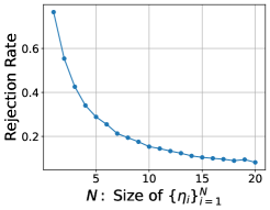
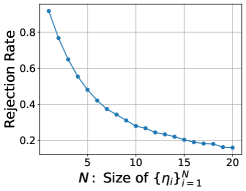
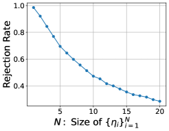
(a) $\eta=0.5$	(b) $\eta=1.0$	(c) $\eta=2.0$

Figure 6: Illustration of the rejection rate by setting $\{\eta_{i}\}_{i=1}^{N}$, where $\eta_{i}=N\eta/i$. The model follows the setting of Figure 1, where we choose Gaussian mixture as $\pi_{0}$ and the preference is mathematically captured by setting $r$ as linearly dependent on $a$, with $r=[1,0]^{\top}a$ and $\eta=1$ for $\pi_{r}$.

where $\eta_{0}=\infty$ (i.e., $\pi_{0}$), $\eta_{N}=\eta$. The high-level intuition is that while approximating $\pi_{r}$ from $\pi_{0}$ is hard, approximating $\pi_{0}\exp(\frac{1}{\eta_{i}}r)$ with $\pi_{0}\exp(\frac{1}{\eta_{i-1}}r)$ is much easier. Therefore, we can do the rejection sampling step by step. Considering the case $\mathbb{E}_{a\sim\pi_{0}(a|x)}\exp(\eta^{-1}r(x,a))=\exp(-\eta^{-1}(r_{x}-R(x)))$, by choosing $N=[r_{x}/\eta]+1$ steps, the acceptance rate at each step becomes an $O(1)$ probability $\exp(-\frac{r_{x}}{\eta([r_{x}/\eta]+1)})>\exp(-1)>0.367$. The acceptance rate can be exponentially increased with the number of steps, i.e., $N$ steps correspond to an $\exp(N)$ increase in the acceptance rate. We also provide a numerical example in the Appendix (Figure 6).

One concern may be on the additional computations introduced by the multi-step approximations. However, in practice, the KL coefficient $\eta$ is also tuned as a hyper-parameter in an outer loop of the proposed framework (Huggingface, 2023) to achieve the best performance. The Algorithm 3 provides us with a sequence of models associated with different $\eta_{i}$, which exactly allows for further model selection via hyper-parameter tuning of $\eta$. In view of this, the Algorithm 3 does not introduce overhead in computation.

5.3 Algorithmic Simplicity and Data Coverage

We note that all the three settings: offline, online (Appendix B), and hybrid learning are complementary to each other and hold their own values. For instance, collecting new and online human feedback can be expensive for most of the developers and in this case, only offline learning is feasible. One appealing choice is to leverage AI feedback (Bai et al., 2022b), which is much cheaper than human feedback. However, for tasks with customized needs or requiring expertise, we may only query feedback from specific users or experts, whose preference is distinct from AI.

Meanwhile, the hybrid learning offers simplicity in algorithmic design, at the cost of demand for a high-quality $\mathcal{D}_{\mathrm{off}}$. In comparison, the online learning starts from scratch, but the choice of the enhancer is challenging because for the neural network, the uncertainty estimators do not admit a closed-form. In practice, we typically resort to heuristic methods (Wu et al., 2021b; Coste et al., 2023) to estimate the uncertainty. As the advantage of a pessimistic MLE in RLHF has been showcased in a large amount of work (e.g., Christiano et al., 2017; Ziegler et al., 2019; Gao et al., 2023; Zhu et al., 2023a; Coste et al., 2023; Shin et al., 2023), we do not leverage pessimism in subsequent experiments but focus on verify the effectiveness of the proposed multi-step approximation approach. For the online setting, the uncertainty estimation seems to be more challenging. We will discuss the potential ways to implement the uncertainty-aware algorithms in Appendix E.3 and defer a comprehensive empirical study to future study.

Algorithm 4 Hybrid GSHF (Practical Implementation)

1:  Input: Offline dataset $\mathcal{D}_{\mathrm{off}}$, KL regularization $\eta>0$, Online iterations $T$, batch size $m$, $\pi_{\mathrm{ref}}$, $\mathcal{D}^{0}=\emptyset$.

2:  for $t=1,2,\cdots,T$ do

3:     Let $r^{t}$ denote the MLE estimator of the likelihood given in Equation (3) based on $\mathcal{D}_{\mathrm{off}}$ and $\mathcal{D}^{1:t-1}$.

4:     Use DPO to train $\pi_{t}$ on $\mathcal{D}_{\mathrm{off}}$ and $\mathcal{D}^{1:t-1}$ so that $\pi_{t}\approx\pi_{r^{t}}(\cdot|x)\propto\pi_{0}(\cdot|x)\cdot\exp\Big{(}\frac{1}{\eta}r^{t}(x,\cdot)\Big{)}$;

5:     Observe $x_{t,i}\sim d_{0}$, sample $a_{t,i}^{1}\sim\pi_{t}$ and $a_{t,i}^{2}\sim\pi_{\mathrm{ref}}$, receive human feedback for all $i\in[m]$, and collect them as $\mathcal{D}^{t}$.

6:  end for

7:  Output: the best model in $\pi_{1:T}$ by a validation set.

6 Experiments

In this section, we verify the effectiveness of the Algorithm 3 and Algorithm 4 by real-world RLHF experiments.

6.1 Experiments Setup

Model, and Task. We use the Open-LLaMA-3B-V2 (Geng & Liu, 2023) as the pretrained model and use the helpful subset of the Anthropic HH-RLHF dataset (Bai et al., 2022a) (see Table 4 for a sample example). We preprocess the dataset to get $103$K training set and $5$K test set, with details in Appendix H.1. We also sample a subset of the UltraFeedback (Cui et al., 2023), consisting of $5$K prompts, as another out-of-distribution (OOD) test set. Meanwhile, the UltraRM-13B (Cui et al., 2023) will be used as the ground truth reward model, also referred to as the gold reward, which is trained on a mixture of UltraFeedback, Anthropic HH-RLHF, and other open-source datasets based on LLaMA2-13B. For all the experiments, we fix the KL penalty in the learning target Equation (2) as $\eta=0.1$.

Offline Data $\mathcal{D}_{\mathrm{off}}$ Generation and Initial Checkpoint. Following Gao et al. (2023); Coste et al. (2023), we use the training prompts to generate responses by an Open-LLaMA-3B-V2 model that is fine-tuned on the preferred responses of the original HH-RLHF dataset. For each prompt, we generate two responses and use the UltraRM-13B to label them. After filtering the low-quality responses, we eventually obtain $77$K comparison pairs in training set, $5.6$K pairs as the validation set. We also set $20$K samples as the “SFT” split to get the RLHF starting checkpoint $\pi_{0}$.

Models	Settings	Gold Reward	Gold Win Rate	GPT4 Eval	OOD Gold Reward	Difference $\Delta\downarrow$	OOD Gold Win Rate	OOD GPT4 Eval
SFT	Offline	$0.27$	-	-	-0.21	0.48	-	-
DPO	Offline	2.15	0.5	0.5	1.71	0.44	0.5	0.5
RSO	Offline	2.25	0.54	0.53	1.89	0.36	0.55	0.52
Offline GSHF	Offline	2.59	0.63	0.57	2.41	0.18	0.64	0.60
Hybrid GSHF	Hybrid	2.67	0.67	0.65	2.46	0.21	0.66	0.59

Table 1: The evaluation results of the models from different RLHF algorithms. The gold rewards are computed on the test split with 5K prompts and the GPT4 evaluations are with 100 randomly sampled test prompts, with the DPO as baseline. We use 5K prompts from the UltraFeedback to compute the OOD reward and $\Delta$ is the difference between the in-domain test reward and the OOD one. We count GPT4 evaluation score as $\text{win}\times 1+\text{tie}\times 0.5$ and provide the details in Appendix H.

Setup of offline learning and hybrid learning. For offline learning, we learn from the offline dataset $\mathcal{D}_{\mathrm{off}}$, and cannot further query human feedback in the training though it is possible to leverage the model itself to generate more responses. For hybrid learning, we start with a subset of $\mathcal{D}_{\mathrm{off}}$, consisting of 25K comparison pairs, and then fix the budget of online human feedback as 52K, leading to a total number of queries consistent with the offline learning for a fair comparison. For all the hybrid algorithms, we will iterate for three steps.

Method, Competitor and Evaluation. In our experiments, we investigate (1) Offline GSHF; (2) Hybrid GSHF; and use (3) SFT on the preferred samples, (4) DPO (Rafailov et al., 2023), (5) RSO (Liu et al., 2023a) as the baselines. The GSHF is implemented by DPO to approximate Oracle 2.2. The representative models of different RLHF methods will be measured by the gold reward of UltraRM-13B and the KL divergence $\mathbb{E}_{x\sim d_{0}}D_{\mathrm{KL}}(\pi(\cdot|x)\|\pi_{0}(\cdot|x))$, which are both evaluated on the split test set.

Stronger DPO Model with Gold RM for Model Selection. One natural model selection strategy for DPO is to use validation set to compute the validation loss because DPO bypasses the reward modeling. Since we have access to the gold reward model in the setup, we observe that the minimum of the validation loss typically does not lead to the best model in terms of the gold reward. Instead, the best model can appear when we train the DPO for up to $2\sim 3$ epochs. This is similar to the observation in Tunstall et al. (2023), where the authors found that overfitting the preference dataset within certain limit does not hurt the model performance (gold reward) and the strongest model was obtained with 3 epochs of DPO training. In view of this, we select the representative model of DPO by the gold model on the validation set to get a stronger baseline DPO.

6.2 Main Results

We present the main results in this subsection and defer implementation details to Appendix H. We report the gold rewards and the GPT4 evaluations compared to the DPO baseline in Table 1. As we can see, DPO, RSO, and GSHF significantly outperform the SFT baseline, and the GSHF algorithms further outperform the stronger baselines including both DPO and RSO in terms of gold reward, and GPT4 evaluations. In particular, the GSHF algorithms tend to be more robust in the face of OOD data, as they achieve a much smaller $\Delta$ compared to other RLHF algorithms.

In addition to the theoretical result provided in this paper, we may also intuitively justify the improvements achieved by the GSHF algorithm (as well as RSO) compared to DPO by noting that they use different data sources for the preference learning thus providing a better coverage of the state-action space. We would like to share some thoughts with more details between the coverage condition and the success of preference learning in Appendix E.

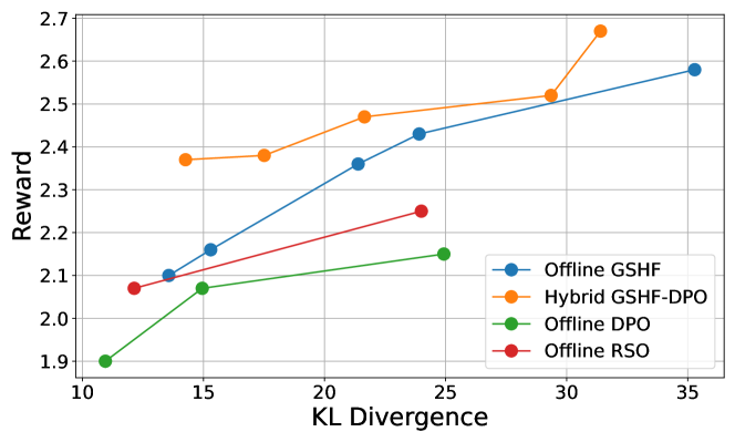
Figure 2: The figure of Reward-KL trade-off. Both the KL divergence and the gold reward are tested on the hand-out test set. The rightest point is the highest gold reward that can be achieved by the RLHF algorithm.

Reward-KL Trade-off. Since all the considered RLHF algorithms (except SFT) share the same KL-constraint reward optimization target in Equation (2), we first investigate the trade-off between the gold reward and the KL divergence achieved by the different RLHF algorithms and plot the curve in Figure 2. As we can see, both the Offline GSHF and the Hybrid GSHF significantly outperform the strong baselines DPO, and RSO by achieving a much higher reward, for a fixed KL level.

The Power of Exploration. We compare different iterations of Hybrid GSHF in Figure 3. For each iteration, we evaluate the models every 400 training steps and plot the representative models. Clearly, the previous iteration is strictly dominated by the subsequent one in terms of the frontier. This demonstrates the significant improvements achieved by further iterating DPO with online data. Notably, compared to offline DPO which uses more offline data than the iteration 1, leveraging online data proves to be far more efficient, as evidenced by the enhanced frontier of the reward-KL trade-off.

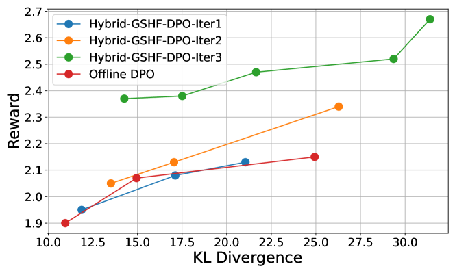
Figure 3: The Reward-KL trade-off curves of different iterations of Hybrid GSHF. The rightest point is the highest gold reward that can be achieved in that round.

Performance Comparison Under Distribution Shift. We investigate the performance of the resulting models from different alignment algorithms under distribution shift. To this end, we sample a subset of the UltraFeedback (Cui et al., 2023), consisting of $5$K prompts, as our out-of-distribution (OOD) test set. The performance results of representative models are detailed in Table 1, and the trade-off between reward and KL divergence on this OOD test set is illustrated in Figure 4. It is observed that all models exhibit a decline in performance compared to the in-domain scenario. In comparison, the Hybrid GSHF and Offline GSHF are more stable in the face of the distribution shift because they achieve a smaller $\Delta$, which is the difference between in-domain and OOD rewards. Regarding the reward-KL trade-off, consistent with in-domain results, the GSHF algorithms outperform the baseline DPO and RSO models in producing a more efficient frontier. In particular, the Hybrid GSHF achieves the best performance, indicating the advantage of online exploration compared to the offline learning.

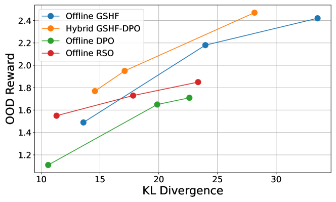
Figure 4: The figure of Reward-KL trade-off on the OOD prompt set from Ultra-Chat. The rightest point is the highest OOD gold reward that can be achieved by the RLHF algorithm.

Performance Comparison Under Different Sampling Temperatures. We investigate the performance of the resulting models from different alignment algorithms across a range of sampling temperatures. We report the test gold reward with respect to the sampling temperature in Figure 5. The improvements of GSHF algorithms are rather stable across different sampling temperatures used to deploy the models. For all the models, a temperature of 0.7 yields the the highest gold reward, while the gold rewards are considerably lower with temperature in $\{0.2,0.5,1.0\}$. An exception is observed with the Offline RSO, which maintains robustness when the temperature is reduced from 1.0 to 0.7. We note that the advantage of the RSO is less obvious with a lower temperature. Conversely, both Offline GSHF and Hybrid GSHF models consistently surpass the baseline DPO and RSO models across various sampling temperatures. Notably, Hybrid GSHF shows more advantages over the Offline GSHF with a lower temperature, potentially indicating the benefits of online exploration.

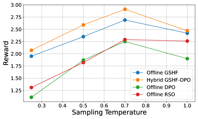
Figure 5: The gold reward with respect to the sampling temperature. The gold reward is tested on the hand-out test set.

Length Bias. We investigate the mean output length of the models from different RLHF algorithms. We observe that as the Hybrid GSHF iterates, the average output lengths increases: from 161 in the first iteration, to 243 in the second, and 263 in the third. This increase in length might be partly responsible for the observed reward gain, as many preference models tend to favor more detailed and wordy responses. In comparison, the average output lengths for DPO, RSO, and Offline GSHF are 241, 275, and 240, respectively. Though there is a trend towards longer responses in later iterations of the Hybrid GSHF model, we notice that the final output length of the Hybrid GSHF model does not significantly exceed that of DPO and RSO. In practice, however, the reward (signal) hacking is the fundamental issue of RLHF (Casper et al., 2023). Therefore, it may be beneficial to integrate additional strategies such as early stopping, replay, and a thorough validation process to ensure the selection of the most effective model during the training process.

7 Conclusion

In this paper, we formulate the real-world RLHF process as a reverse-KL regularized contextual bandit problem. Compared to existing theoretical RLHF frameworks, the proposed framework admits a stochastic optimal policy, that more accurately reflects the dynamics of foundation generative models and aligns closely with current alignment practices (Ouyang et al., 2022; Bai et al., 2022a; Rafailov et al., 2023). We design statistically efficient algorithms in offline, online, and hybrid settings, featuring the standard ideas of pessimism and optimism in the new framework, while also handling the distinct challenges of preference learning as well as the newly introduced KL constraint with distinct algorithmic designs.

The theoretical findings also sheds light on innovative pathways for practical algorithmic development, as we move toward implementations of the information-theoretical algorithms in Section 5. The practical implementations of the proposed algorithms outperform strong baselines like DPO and RSO in real-world alignment of LLMs.

Appendix A Notation Table and Backgrounds

To improve the readability of this paper, we provide a Table 2 for the notations used in this paper. We also provide an introduction to the eluder-type techniques and the rejection sampling for completeness.

Notation	Description
$\left\langle z_{1},z_{2}\right\rangle$	The inner product of two vectors $z_{1}^{\top}z_{2}$.
$\|z\|_{\Sigma}$	The induced norm $\sqrt{z^{\top}\Sigma z}$.
$\mathcal{X},\mathcal{A}$	The state (prompt) space and the action (response) space.
$\phi(x,a),\theta$	The feature map and parameter of the linear parameterization in Assumption 2.1.
$d$	The dimension of the feature vector.
$\pi,\Pi$	Policy and policy class.
$\ell_{\mathcal{D}}$	The log-likelihood of the BT model on $\mathcal{D}$ defined in Equation (3).
$y\in\{0,1\}$	Preference signal.
$J(\pi)$	The KL-regularized target defined in Equation (2).
$\eta$	The coefficient of KL penalty, defined in Equation (2).
$d_{0}$	Distribution of state (prompt).
$B,\gamma$	Regularization constant: $\|\theta\|\leq B,\gamma=1/(2+\exp(-B)+\exp(B))$.
$\Theta(B)$	$\{\theta\in\mathbb{R}^{d}:\|\theta\|\leq B\}$.
$\mathcal{D}_{\mathrm{off}},\mathcal{D}^{t}$	The offline dataset and the dataset collected in online iteration $t$.
$\Sigma_{\mathrm{off}},\Sigma_{t}$	The covariance matrix with $\mathcal{D}_{\mathrm{off}}$ and $\mathcal{D}^{t}$.
$\sigma(\cdot)$	$\sigma(z)=1/(1+\exp(-z))$ is the sigmoid function.
$C_{\mathrm{cov}}(\mathcal{D}_{\mathrm{off}},\pi_{\mathrm{ref}},\alpha)$	The coverage of the offline dataset defined in Definition 4.1.
Rejection Sampling	See Appendix A.2 for an introduction.
Best-of-n Policy	See Appendix A.2 for an introduction.

Table 2: The table of notations used in this paper.

A.1 Covariance Matrix and Generalization

Before we continue to prove the main results of this paper, we would like to briefly illustrate the high-level intuitions why the algorithmic design and analysis are centered on the covariance matrix. Given a preference dataset $\mathcal{D}$, and a fixed $\lambda>0$, we denote $\Sigma_{\mathcal{D}}$ as

$$\Sigma_{\mathcal{D}}:=\lambda I+\sum_{(x,a^{1},a^{2})\in\mathcal{D}}\big{(}\phi(x,a^{1})-\phi(x,a^{2})\big{)}\big{(}\phi(x,a^{1})-\phi(x,a^{2})\big{)}^{\top}.$$

Then, the in-sample error on the observed data in $\mathcal{D}$ is given by

$$\|\theta_{1}-\theta_{2}\|_{\Sigma_{\mathcal{D}}}^{2}=\lambda\|\theta_{1}-\theta_{2}\|^{2}+\sum_{(x,a^{1},a^{2})\in\mathcal{D}}\Big{(}\big{(}r_{\theta_{1}}(x,a^{1})-r_{\theta_{1}}(x,a^{2})\big{)}-\big{(}r_{\theta_{2}}(x,a^{1})-r_{\theta_{2}}(x,a^{2})\big{)}\Big{)}^{2},$$

where we additionally add a regularization term $\lambda\|\theta_{1}-\theta_{2}\|^{2}$. Meanwhile, if we test the hypothesis $(\theta_{1}-\theta_{2})$ on a newly observed data, the out-of-sample error would be given by $|\left\langle\theta_{1}-\theta_{2},\phi(x,a^{1})-\phi(x,a^{2})\right\rangle|.$ The ideal case would be that we can infer the out-of-sample error via the in-sample error, so we look at the ratio between them:

$$\frac{|\left\langle\theta_{1}-\theta_{2},\phi(x,a^{1})-\phi(x,a^{2})\right\rangle|}{\|\theta_{1}-\theta_{2}\|_{\Sigma_{\mathcal{D}}}}\leq\frac{\|\phi(x,a^{1})-\phi(x,a^{2})\|_{\Sigma_{\mathcal{D}}^{-1}}\cdot\|\theta_{1}-\theta_{2}\|_{\Sigma_{\mathcal{D}}}}{\|\theta_{1}-\theta_{2}\|_{\Sigma_{\mathcal{D}}}}=\|\phi(x,a^{1})-\phi(x,a^{2})\|_{\Sigma_{\mathcal{D}}^{-1}},$$

where we take a square root on the in-sample error to keep them being of the same order and use Cauchy-Schwarz inequality (Lemma G.2). Here, the $\|\phi(x,a^{1})-\phi(x,a^{2})\|_{\Sigma_{\mathcal{D}}^{-1}}$ is referred to as the elliptical potential in the literature of linear function approximation (Abbasi-Yadkori et al., 2011). The elliptical potential can be viewed as the uncertainty of $\phi(x,a^{1})-\phi(x,a^{2})$, given the historical samples in $\mathcal{D}$, and can be used to guide our exploration. The complexity of the reward model space is characterized by the following fact:

Lemma A.1 (Elliptical potential is usually small (Hu et al., 2022)).

For a fixed $\lambda>0$ and $\{z_{t}\}_{t=1}^{T}\subset\mathbb{R}^{d}$ with $\|z_{t}\|\leq 1$, we define $Z_{t}=\lambda I+\sum_{s=1}^{t-1}z_{s}z_{s}^{\top}$. Then, for any constant $c>0$, $\|z_{t}\|_{Z_{t}^{-1}}>c$ happens at most $\frac{3d}{\log(1+c^{2})}\log\Big{(}1+\frac{1}{\lambda\log(1+c^{2})}\Big{)}.$

The ratio between the out-of-sample error and the in-sample error in the linear case can be readily generalized to the general function approximation using the variant of eluder dimension considered in Gentile et al. (2022); Zhang (2023); Ye et al. (2023); Agarwal et al. (2023), which essentially states that there is some low-rank structure in the reward model space so the generalization is limited (the elliptical potential cannot be large for too many times). Moreover, if we can effectively estimate the in-sample error from the preference data, by Lemma A.1, we can infer the out-of-sample error safely most of the time. Such an in-sample error estimation is provided in Lemma G.3. Essentially, the eluder-type complexity measures and techniques reduce the learning problem to an online supervised learning (in-sample error estimation and minimization) (Zhong et al., 2022).

A.2 Rejection Sampling

We briefly introduce the rejection sampling in this subsection. We first remark that in the literature, many papers use this terminology to refer best-of-n policy (Touvron et al., 2023), which can be different from the notion of rejection sampling here. Specifically, the best-of-n policy takes a base policy $\pi$ and a reward function $r$ as the input, and output a new policy $\widetilde{\pi}$: for each $x\in\mathcal{X}$, we sample $n$ independent policies from $\pi$ and output the one with the highest reward measured by $r$. In what follows, we introduce the rejection sampling.

Rejection sampling, a widely utilized method in Monte Carlo tasks, is designed to sample from a target distribution using samples from a proposal distribution and a uniform sampler (Neumann, 1951). This technique is applicable when the density ratio between the target distribution $q$ and the proposal distribution $p$ is bounded, satisfying $q(x)/p(x)\leq M$ for all $x\in\mathcal{X}$. In practical implementation, $n$ samples are drawn from the proposal distribution $p$. Each sample, denoted as $x\sim p$, is accepted with a probability $r=\frac{q(x)}{Mp(x)}$. This acceptance is determined by evaluating whether $u<r$, where $u$ is a number drawn from a uniform distribution $U[0,1]$. The accepted samples $\widetilde{x}$ are then representative of the target distribution $q$.

The primary challenge in rejection sampling is its low acceptance rate, particularly problematic for high-dimensional data due to the curse of dimensionality, where the density ratio often scales with $\exp(d)$. This issue persists even in low-dimensional scenarios, as a large density ratio $M$ can drastically reduce acceptance rates. The method is most efficient when $p$ closely approximates $q$, leading to $M\approx 1$.

Appendix B (Batch) Online Learning with Enhancer

In this section, we develop the online framework of the KL-constraint contextual bandit, that is missing in the main paper.

The mathematical formulation of the online learning is almost the same as the hybrid case, except that we now start from scratch instead of the offline dataset. Consider the batch online setting of $T$ batches with fixed batch size $m$. At the beginning of each batch $t\in[T]$, An agent updates the policies $\pi_{t}^{1}$ and $\pi_{t}^{2}$. Then, $m$ prompts $\{x_{t,i}\}_{i=1}^{m}$ are sampled from $d_{0}$. Based on each prompt $x_{t,i}$, two responses $(a_{t,i}^{1},a_{t,i}^{2})$ are generated from two policies $(\pi_{t}^{1},\pi_{t}^{2})$, and a human preference signal $y_{t,i}\in\{0,1\}$ is yielded according to the ground-truth BT model.

B.1 Batch Online Learning

We first consider the case of $m>1$, which leads to a more sparse update of the model. Our goal is also to design a sample-efficient algorithm, which finds a policy $\hat{\pi}$ so that the suboptimality $J(\pi^{*})-J(\hat{\pi})<\epsilon$ with the number of samples polynomial in the accuracy number $1/\epsilon$, feature dimension $d$, and other problem-dependent parameters. In practical applications, it is observed that the diversity of the outputs is critical, and the response pairs $(a^{1}_{t},a^{2}_{t})$ are recommended to be collected by different model variants with different temperature hyper-parameter (Touvron et al., 2023). To understand this choice, we recall the decomposition Lemma 2.3 and Lemma 2.4 to obtain for each batch $t\in[T]$

$$J(\pi^{*})-J(\pi_{t}^{1})$$

$$=\mathbb{E}_{x_{t}\sim d_{0}}\Big{[}{\mathbb{E}_{\pi^{*}}[r^{*}(x_{t},a)-\hat{r}(x_{t},a)]}+{\mathbb{E}_{\pi_{t}^{1}}[\hat{r}(x_{t},a)-r^{*}(x_{t},a)]}-\eta\cdot\mathbb{E}_{x_{t}\sim d_{0}}\big{[}D_{\mathrm{KL}}(\pi^{*}(\cdot|x_{t})\|\pi_{t}^{1}(\cdot|x_{t}))\Big{]}$$

$$=\mathbb{E}_{x_{t}\sim d_{0}}\Big{[}\left\langle\hat{\theta}-\theta^{*},\phi(x_{t},\pi_{t}^{1})-\phi(x_{t},\pi^{*})\right\rangle\Big{]}-\eta\cdot\mathbb{E}_{x_{t}\sim d_{0}}\big{[}D_{\mathrm{KL}}(\pi^{*}(\cdot|x_{t})\|\pi_{t}^{1}(\cdot|x_{t}))\Big{]}.$$ (7)

The main technical challenge is to relate the uncertainty of $\phi(x_{t},\pi_{t}^{1})-\phi(x_{t},\pi^{*})$ (analysis target) to the uncertainty of $\phi(x_{t},\pi_{t}^{1})-\phi(x_{t},\pi_{t}^{2})$ (the pair to collect data). Our algorithmic idea is built on optimism and non-symmetric structures. We present the complete algorithm in Algorithm 5. The main agent $\pi_{t}^{1}$ always takes the policy induced by $r^{t}$ from Oracle 2.2. On the other hand, the second agent $\pi_{t}^{2}$, referred to as the enhancer, seeks to maximize the uncertainty (similar to the practical choice of different model variants and temperature) for the fixed $\pi_{t}^{1}$, thus facilitating the learning of the main agent (similar idea was considered in the study of two-player zero-sum Markov game (Jin et al., 2021a; Huang et al., 2021; Xiong et al., 2022b)). In this case, the uncertainty compared to $\pi^{*}$ is upper bounded by that of $\pi_{t}^{2}$, which is referred to as the principle of optimism in the literature (Auer et al., 2002). Notably, in contrast to the case of Markov game (Jin et al., 2021a; Huang et al., 2021; Xiong et al., 2022b), the enhancer also converges to $\pi^{*}$ in terms of the metric of $J(\pi)$. We borrow the terminology of the main agent and enhancer to stress the non-symmetric algorithmic structure. Moreover, if we just regard the enhancer $\pi_{t}^{2}$ as an auxiliary policy and only care about the performance of $\pi_{t}^{1}$, there is no need to maintain the confidence set $\Pi_{t}$. Due to the realizability: $\pi^{*}\in\Pi$, we can construct $\pi_{t}^{2}$ as the solution of the following unconstrained problem:

$$\pi_{t}^{2}=\mathop{\mathrm{argmax}}_{\pi_{t}^{2}\in\Pi}\sum_{i=1}^{m}\Gamma(x_{t,i},\pi_{t}^{1},\pi_{t}^{2},\mathcal{D}^{1:t-1}),$$ (8)

where the uncertainty bonus will be specified later. Note that in Algorithm 5, we formulate that the agent first observes $m$ prompts and then establishes the enhancer. This is only for simplicity of analysis so that we can estimate the uncertainty and obtain the enhancer by maximizing the estimation. If we consider the standard online contextual bandit, we can first collect $m$ contexts, and estimate the uncertainty based on them. Then, for the next $m$ contexts, we interact with the environment in a strictly sequential manner using the policies determined by the first $m$ contexts. This will only roughly incur a constant factor $2$ in the final sample complexity.

Algorithm 5 Online GSHF with Enhancer

1:  Input: $\Pi,\mathcal{D}^{0}=\emptyset,m\geq 1$.

2:  for $t=1,2,\cdots,T$ do

3:     Observe $m$ independent prompts $\{x_{t,i}\}_{i=1}^{m}\sim d_{0}$;

4:     Compute the MLE-based reward $r^{t}$ based on $\mathcal{D}^{1:t-1}$;

5:     Compute the policy $\pi_{t}^{1}$ by calling the oracle in Assumption 2.2 with $r^{t}$;

6:     Construct the confidence set of the policy as in Lemma B.1;

7:     Compute the enhancer policy $\pi_{t}^{2}$ as in Equation (8);

8:     Independently sample actions $a^{1}_{t,i}\sim\pi_{t}^{1}(\cdot|x_{t,i})$, $a^{2}_{t,i}\sim\pi_{t}^{2}(\cdot|x_{t,i})$ and receive human feedback $y_{t,i}$, and collect $\mathcal{D}^{t}=\{(x_{t,i},a^{1}_{t,i},a^{2}_{t,i},y_{t,i})\}_{i=1}^{m}$

9:  end for

To achieve optimism, we need to maintain a confidence set, that contains the $\pi^{*}$ for all iterations with high probability. The constructions of the confidence set are different compared to the dueling RL (Faury et al., 2020; Pacchiano et al., 2021) due to the reverse-KL regularized contextual bandit formulation, as well as the non-symmetric structure in our algorithm. We summarize the confidence set construction for the online setting in the following lemma.

Lemma B.1 (Confidence set).

For the linear model in Assumption 2.1, given the policy of the main agent $\pi_{t}^{1}$, we consider the following confidence set with $\beta=O\big{(}\sqrt{\frac{d\log(T/\delta)}{\gamma^{2}m}}\big{)}$:

$$\Pi_{t} =\Big{\{}\widetilde{\pi}\in\Pi:\beta\sum_{i=1}^{m}\|\phi(x_{t,i},\widetilde{\pi})-\phi(x_{t,i},\pi_{t}^{1})\|_{\Sigma_{t,m}^{-1}}-\eta\sum_{i=1}^{m}D_{\mathrm{KL}}(\widetilde{\pi}(\cdot|x_{t,i})\|\pi_{t}^{1}(\cdot|x_{t,i}))\geq 0\Big{\}},$$

where we define

$$\Sigma_{t,m}=\lambda I+\frac{1}{m}\sum_{i=1}^{t-1}\sum_{j=1}^{m}(\phi(x_{i,j},a_{i,j}^{1})-\phi(x_{i,j},a_{i,j}^{2}))(\phi(x_{i,j},a_{i,j}^{1})-\phi(x_{i,j},a_{i,j}^{2}))^{\top}.$$

Then, with probability at least $1-\delta$, we know that $\pi^{*}\in\Pi_{t}$ for all $t\in[T]$.

We defer the proof to Appendix B.3. Intuitively, the enhancer aims to maximize the uncertainty of the feature difference, thus facilitating the learning of the main agent. In particular, the largest cost of KL divergence scales with the uncertainty of the difference, demonstrating the trade-off between the two considerations. Since $\pi^{*}\in\Pi_{t}$, we can upper-bound the first term on the right-hand side of Equation (B.1) by $\beta\mathbb{E}_{x_{t}\sim d_{0}}\|\phi(x_{t},\pi_{t}^{1})-\phi(x_{t},\pi_{t}^{2})\|_{\Sigma_{t,m}^{-1}}$, which can be further bounded by elliptical potential lemma. Hence, we can obtain the probably approximately correct (PAC) learning result in the following theorem.

Theorem B.2.

For any $\epsilon>0$, we set the batch size $m=d/(\gamma^{2}\epsilon^{2})$. Under Assumption 2.1 with the uncertainty estimator defined as

$$\Gamma(x,\pi_{t}^{1},\pi_{t}^{2},\mathcal{D}^{1:t-1})=\|\phi(x,\pi_{t}^{1})-\phi(x,\pi_{t}^{2})\|_{\Sigma_{t,m}^{-1}},$$ (9)

with $\beta:=O\big{(}\sqrt{\frac{d\log(T/\delta)}{\gamma^{2}m}}\big{)}$ and $\lambda=\Theta\big{(}d\log(T/\delta)/(m\gamma^{2}B^{2})\big{)}$, after $T=\min\{n\in\mathbb{N}^{+}:n\geq d\log(n)\}$ iterations, we have with probability at least $1-3\delta$, there exists a $t_{0}\in[T]$,

$$J(\pi^{*})-J(\pi^{1}_{t_{0}})\lesssim\epsilon-\eta\cdot\mathbb{E}_{x_{t_{0}}\sim d_{0}}\big{[}D_{\mathrm{KL}}(\pi^{*}(\cdot|x_{t_{0}})\|\pi^{1}_{t_{0}}(\cdot|x_{t_{0}}))\big{]}\Big{)},$$

where the number of collected samples is at most $mT=\widetilde{O}\Big{(}\frac{d^{2}}{\gamma^{2}\epsilon^{2}}\Big{)}.$

Theorem B.2 reveals a key characteristic of reward modeling: the sample complexity is dependent on the complexity of the reward model rather than the generative models. For simple reward functions, such as sentiment or politeness evaluation, the required function class is substantially smaller compared to the generative model. We now present the proof of the theorem.

Proof of Theorem B.2.

Recall the definition of the covariance matrix:

$$\Sigma_{t,m}=\lambda I+\frac{1}{m}\sum_{i=1}^{t-1}\sum_{j=1}^{m}(\phi(x_{i,j},a_{i,j}^{1})-\phi(x_{i,j},a_{i,j}^{2}))(\phi(x_{i,j},a_{i,j}^{1})-\phi(x_{i,j},a_{i,j}^{2}))^{\top}.$$

Then, by invoking Lemma G.3 for $\theta_{t}$ with $\Sigma_{\mathcal{D}}=m\Sigma_{t,m}$ and $\lambda^{\prime}=m\lambda$, we have with probability at least $1-\delta$, for any $t\in[T]$,

$$\|\theta^{t}-\theta^{*}\|_{\Sigma_{t,m}}= \frac{1}{\sqrt{m}}\|\theta^{t}-\theta^{*}\|_{\Sigma_{\mathcal{D}}}$$

$$\leq \frac{C}{\sqrt{m}}\sqrt{\frac{d+\log(T/\delta)}{\gamma^{2}}+m\lambda B^{2}}$$

$$= C\sqrt{\frac{d+\log(T/\delta)}{\gamma^{2}m}+\lambda B^{2}}.$$ (10)

Let

$$\widetilde{\Sigma}_{t}=\lambda I+\sum_{i=1}^{t-1}\mathbb{E}_{x\sim d_{0},a^{1}\sim\pi_{i}^{1},a^{2}\sim\pi_{i}^{2}}\left[(\phi(x_{t},a^{1})-\phi(x_{t},a^{2}))(\phi(x_{t},a^{1})-\phi(x_{t},a^{2}))^{\top}\right].$$

Now, by elliptical potential lemma (Lemma G.4), we have

$$\sum_{t=1}^{T}\log\big{(}1+\mathbb{E}_{x_{t}\sim d_{0}}\|\phi(x_{t},\pi_{t}^{1})-\phi(x_{t},\pi_{t}^{2})\|_{\widetilde{\Sigma}_{t}^{-1}}^{2}\big{)}\leq \sum_{t=1}^{T}\log\big{(}1+\mathbb{E}_{x_{t}\sim d_{0},a^{1}\sim\pi_{t}^{1},a^{2}\sim\pi_{t}^{2}}\|[\phi(x_{t},a^{1})-\phi(x_{t},a^{2})]\|_{\widetilde{\Sigma}_{t}^{-1}}^{2}\big{)}$$

$$\leq \log\frac{\det(\widetilde{\Sigma}_{T})}{\det(\lambda I)}$$

$$\leq d\log(1+TL^{2}/\lambda d):=\gamma_{T}(\lambda).$$

Since each term on the left-hand side is positive, we know that there exists at least a $t_{0}\in[T]$, the value is smaller or equal than the average value:

$$\log\big{(}1+\psi_{t_{0}}^{2}\big{)}\leq\frac{1}{T}\gamma_{T}(\lambda),$$

where we use the short-hand notation $\psi_{t}=\mathbb{E}_{x_{t}\sim d_{0}}\|\phi(x_{t},\pi_{t}^{1})-\phi(x_{t},\pi_{t}^{2})\|_{\widetilde{\Sigma}_{t}^{-1}}$. It is equivalent to

$$\psi_{t_{0}}^{2}\leq\exp\big{(}\frac{\gamma_{T}(\lambda)}{T}\big{)}-1.$$

We now consider the suboptimality at iteration $t_{0}$:

$$J(\pi^{*})-J(\pi^{1}_{t_{0}}) =\mathbb{E}_{x_{t_{0}}\sim d_{0}}\Big{[}\left\langle\theta^{t_{0}}-\theta^{*},\phi(x_{t_{0}},\pi_{t_{0}}^{1})-\phi(x_{t_{0}},\pi^{*})\right\rangle\Big{]}-\eta\mathbb{E}_{x_{t_{0}}\sim d_{0}}\big{[}D_{\mathrm{KL}}(\pi^{*}(\cdot|x_{t_{0}})\|\pi^{1}_{t_{0}}(\cdot|x_{t_{0}}))\big{]}$$

$$\leq\mathbb{E}_{x_{t_{0}}\sim d_{0}}\Big{[}\|\phi(x_{t_{0}},\pi_{t_{0}}^{1})-\phi(x_{t_{0}},\pi^{*})\|_{\Sigma_{t,m}^{-1}}\Big{]}\cdot\|\theta^{t_{0}}-\theta^{*}\|_{\Sigma_{t,m}}-\eta\mathbb{E}_{x_{t_{0}}\sim d_{0}}\big{[}D_{\mathrm{KL}}(\pi^{*}(\cdot|x_{t_{0}})\|\pi^{1}_{t_{0}}(\cdot|x_{t_{0}}))\big{]},$$ (11)

where the inequality uses the Cauchy-Schwarz inequality (Lemma G.2). Then, since the samples $\{x_{t,i}\}_{i=1}^{m}$ are i.i.d and for any $x\in\mathcal{X}$

$$\|\phi(x,\pi_{t_{0}}^{1})-\phi(x_{t_{0}},\pi^{*})\|_{\Sigma_{t,m}^{-1}}\leq\frac{2}{\sqrt{\lambda}},$$

we can use Chernoff bound (Theorem 2.16 of Zhang (2023)) to obtain that with probability at least $1-\delta/2$,

$$\mathbb{E}_{x_{t_{0}}\sim d_{0}}\Big{[}\|\phi(x_{t_{0}},\pi_{t_{0}}^{1})-\phi(x_{t_{0}},\pi^{*})\|_{\Sigma_{t,m}^{-1}}\Big{]}\leq\frac{1}{m}\sum_{i=1}^{m}\|\phi(x_{t,i},\pi_{t_{0}}^{1})-\phi(x_{t,i},\pi^{*})\|_{\Sigma_{t,m}^{-1}}+\sqrt{\frac{\log(2/\delta)}{2m}}.$$

Similarly, we also get with probability at least $1-\delta/2$,

$$\frac{1}{m}\sum_{i=1}^{m}\|\phi(x_{t,i},\pi_{t_{0}}^{1})-\phi(x_{t,i},\pi^{*})\|_{\widetilde{\Sigma}_{t_{0}}^{-1}}\leq\mathbb{E}_{x_{t_{0}}\sim d_{0}}\Big{[}\|\phi(x_{t_{0}},\pi_{t_{0}}^{1})-\phi(x_{t_{0}},\pi^{*})\|_{\widetilde{\Sigma}_{t_{0}}^{-1}}\Big{]}+\sqrt{\frac{\log(2/\delta)}{2m}}$$

We take the two inequalities above back into Equation (B.1) to derive with that probability at least $1-3\delta$,

$$J(\pi^{*})-J(\pi^{1}_{t_{0}})$$

$$\leq\Big{(}\frac{1}{m}\sum_{i=1}^{m}\Big{[}\|\phi(x_{t_{0},i},\pi_{t_{0}}^{1})-\phi(x_{t_{0},i},\pi^{*})\|_{\Sigma_{t_{0},m}^{-1}}\Big{]}+\sqrt{\frac{\log(2/\delta)}{2m}}\Big{)}\cdot\|\theta^{t_{0}}-\theta^{*}\|_{\Sigma_{t_{0},m}}-\eta\mathbb{E}_{x_{t_{0}}\sim d_{0}}\big{[}D_{\mathrm{KL}}(\pi^{*}(\cdot|x_{t_{0}})\|\pi^{1}_{t_{0}}(\cdot|x_{t_{0}}))\big{]}$$

$$\leq\Big{(}\frac{1}{m}\sum_{i=1}^{m}\Big{[}\|\phi(x_{t_{0},i},\pi_{t_{0}}^{1})-\phi(x_{t_{0},i},\pi_{t_{0}}^{2})\|_{\Sigma_{t_{0},m}^{-1}}\Big{]}+\sqrt{\frac{\log(2/\delta)}{2m}}\Big{)}\cdot\|\theta^{t_{0}}-\theta^{*}\|_{\Sigma_{t_{0},m}}-\eta\mathbb{E}_{x_{t_{0}}\sim d_{0}}\big{[}D_{\mathrm{KL}}(\pi^{*}(\cdot|x_{t_{0}})\|\pi^{1}_{t_{0}}(\cdot|x_{t_{0}}))\big{]}$$

$$\leq\Big{(}\frac{\sqrt{3}}{m}\sum_{i=1}^{m}\Big{[}\|\phi(x_{t_{0},i},\pi_{t_{0}}^{1})-\phi(x_{t_{0},i},\pi_{t_{0}}^{2})\|_{\widetilde{\Sigma}_{t_{0}}^{-1}}\Big{]}+\sqrt{\frac{\log(2/\delta)}{2m}}\Big{)}\cdot\|\theta^{t_{0}}-\theta^{*}\|_{\Sigma_{t_{0},m}}-\eta\mathbb{E}_{x_{t_{0}}\sim d_{0}}\big{[}D_{\mathrm{KL}}(\pi^{*}(\cdot|x_{t_{0}})\|\pi^{1}_{t_{0}}(\cdot|x_{t_{0}}))\big{]}$$

$$\leq\Big{(}\sqrt{3}\mathbb{E}_{x_{t_{0}}\sim d_{0}}\Big{[}\|\phi(x_{t_{0}},\pi_{t_{0}}^{1})-\phi(x_{t_{0}},\pi^{*})\|_{\widetilde{\Sigma}_{t_{0}}^{-1}}\Big{]}+2\sqrt{\frac{\log(2/\delta)}{2m}}\Big{)}\cdot\|\theta^{t_{0}}-\theta^{*}\|_{\Sigma_{t_{0},m}}-\eta\mathbb{E}_{x_{t_{0}}\sim d_{0}}\big{[}D_{\mathrm{KL}}(\pi^{*}(\cdot|x_{t_{0}})\|\pi^{1}_{t_{0}}(\cdot|x_{t_{0}}))\big{]}$$

$$\leq C\cdot\Big{(}\sqrt{\exp\big{(}\frac{\gamma_{T}(\lambda)}{T})-1}+2\sqrt{\frac{\log(2/\delta)}{2m}}\Big{)}\sqrt{\frac{d+\log(T/\delta)}{\gamma^{2}m}+\lambda B^{2}}-\eta\mathbb{E}_{x_{t_{0}}\sim d_{0}}\big{[}D_{\mathrm{KL}}(\pi^{*}(\cdot|x_{t_{0}})\|\pi^{1}_{t_{0}}(\cdot|x_{t_{0}}))\big{]},$$ (12)

where the second inequality applies Lemma G.5 with $\lambda=\Omega(d\log(T/\delta)/m)$, and the last inequality uses Equation (B.1). By choosing $T$ satisfying that $T\geq d\log(T)$ and $\lambda=\Theta(d\log(T/\delta)/m\gamma^{2})$, we have

$$J(\pi^{*})-J(\pi^{1}_{t_{0}})=\widetilde{O}\Big{(}\sqrt{\frac{d}{\gamma^{2}m}}-\eta\mathbb{E}_{x_{t_{0}}\sim d_{0}}\big{[}D_{\mathrm{KL}}(\pi^{*}(\cdot|x_{t_{0}})\|\pi^{1}_{t_{0}}(\cdot|x_{t_{0}}))\big{]}\Big{)},$$

which concludes the proof. ∎

B.2 Sequential Online Setting

While we mainly care about finding a good model, with a slightly more involved analysis for the enhancer, we can also derive an upper bound for the average regret as in Pacchiano et al. (2021); Chen et al. (2022):

$$\mathrm{Reg}_{\mathrm{ave}}(T):=\sum_{t=1}^{T}\Big{[}\frac{2J(\pi^{*})-J(\pi_{t}^{1})-J(\pi_{t}^{2})}{2}\Big{]},$$

where we now discuss in the sequential case with $m=1$ in Algorithm 5. We consider two kinds of regrets: (1) cumulative suboptimality for the main policy $\pi_{t}^{1}$ compared to $\pi^{*}$:

$$\mathrm{Reg}(T):=\sum_{t=1}^{T}\big{[}J(\pi^{*})-J(\pi_{t}^{1})\big{]},$$

and (2) the average suboptimality:

$$\mathrm{Reg}_{\mathrm{ave}}(T):=\sum_{t=1}^{T}\big{[}\frac{2J(\pi^{*})-J(\pi_{t}^{1})-J(\pi_{t}^{2})}{2}\big{]}.$$

In this case, our goal is to output a sequence of policy pair $\{\pi_{t}^{1},\pi_{t}^{2}\}_{t=1}^{T}$ so that the regrets $\mathrm{Reg}(T)$ and $\mathrm{Reg}_{\mathrm{ave}}(T)$ are sublinear. To achieve this goal, the enhancer computes its policy by maximizing the uncertainty estimator

$$\pi_{t}^{2}=\mathop{\mathrm{argmax}}_{\pi_{t}^{2}\in\Pi_{t}}\sum_{i=1}^{m}\Gamma(x_{t,i},\pi_{t}^{1},\pi_{t}^{2},\mathcal{D}^{1:t-1}),$$ (13)

where $\mathcal{D}^{1:t-1}=\cup_{s=1}^{t-1}\mathcal{D}^{s}$.

Theorem B.3 (Sequential Online learning).

Under Assumption 2.1 with the uncertainty estimator defined in Equation (9), with $\lambda=\Omega(d\log(T/\delta)/(\gamma^{2}B^{2}))$ and $\beta:=O\big{(}\sqrt{\frac{d\log(T/\delta)}{\gamma^{2}}}\big{)}$, with probability at least $1-2\delta$, the regret of Algorithm 5 with $m=1$ satisfies

$$\mathrm{Reg}_{\mathrm{ave}}(T)\lesssim\sqrt{T\beta^{2}d}-\eta\sum_{t=1}^{T}\mathbb{E}_{x_{t}\sim d_{0}}\big{[}D_{\mathrm{KL}}(\pi^{*}(\cdot|x_{t})\|\pi_{1}^{t}(\cdot|x_{t}))\big{]},$$

which further implies that

$$\mathrm{Reg}(T)\lesssim\sqrt{T\beta^{2}d}-\eta\sum_{t=1}^{T}\mathbb{E}_{x_{t}\sim d_{0}}\big{[}D_{\mathrm{KL}}(\pi^{*}(\cdot|x_{t})\|\pi_{1}^{t}(\cdot|x_{t}))\big{]}.$$

Proof of Theorem B.3.

First, recalling the regret decomposition in Equation (B.1), we deduce that with probability at least $1-\delta$,

$$\sum_{t=1}^{T}\big{[}J(\pi^{*})-J(\pi_{t}^{1})\big{]}$$

$$=\sum_{t=1}^{T}\mathbb{E}_{x_{t}\sim d_{0}}\Big{[}\left\langle\theta^{t}-\theta^{*},\phi(x_{t},\pi_{t}^{1})-\phi(x_{t},\pi^{*})\right\rangle\Big{]}-\eta\sum_{t=1}^{T}\mathbb{E}_{x_{t}\sim d_{0}}\big{[}D_{\mathrm{KL}}(\pi^{*}(\cdot|x_{t})\|\pi_{1}^{t}(\cdot|x_{t}))\big{]}$$

$$\leq\beta\sum_{t=1}^{T}\mathbb{E}_{x_{t}\sim d_{0}}\min\big{\{}1,\|\phi(x_{t},\pi_{t}^{1})-\phi(x_{t},\pi^{*})\|_{\Sigma_{t}^{-1}}\big{\}}-\eta\sum_{t=1}^{T}\mathbb{E}_{x_{t}\sim d_{0}}\big{[}D_{\mathrm{KL}}(\pi^{*}(\cdot|x_{t})\|\pi_{1}^{t}(\cdot|x_{t}))\big{]}$$

$$\leq\beta\sum_{t=1}^{T}\mathbb{E}_{x_{t}\sim d_{0}}\min\big{\{}1,\|\phi(x_{t},\pi_{t}^{1})-\phi(x_{t},\pi_{t}^{2})\|_{\Sigma_{t}^{-1}}\big{\}}-\eta\sum_{t=1}^{T}\mathbb{E}_{x_{t}\sim d_{0}}\big{[}D_{\mathrm{KL}}(\pi^{*}(\cdot|x_{t})\|\pi_{1}^{t}(\cdot|x_{t}))\big{]}$$

$$\leq\beta\sqrt{T\sum_{t=1}^{T}\mathbb{E}_{x_{t}\sim d_{0},(a_{t}^{1},a_{t}^{2})\sim(\pi_{t}^{1},\pi_{t}^{2})}\min\big{\{}1,\|\phi(x_{t},a_{t}^{1})-\phi(x_{t},a_{t}^{2})\|^{2}_{\Sigma_{t}^{-1}}\big{\}}}-\eta\sum_{t=1}^{T}\mathbb{E}_{x_{t}\sim d_{0}}\big{[}D_{\mathrm{KL}}(\pi^{*}(\cdot|x_{t})\|\pi_{1}^{t}(\cdot|x_{t}))\big{]},$$ (14)

where the first inequality uses the Cauchy-Schwarz inequality, Lemma G.3 and reward $r\leq 1$ for any $r\in\mathcal{F}$, the second inequality uses $\pi^{*}\in\Pi_{t}$ according to Lemma B.1, and the last inequality uses the Cauchy-Schwarz inequality and Jensen’s inequality.

Then, we define

$$\bar{\Sigma}_{t}=\sum_{t=1}^{T}\mathbb{E}_{x_{t}\sim d_{0},(a_{t}^{1},a_{t}^{2})\sim(\pi_{t}^{1},\pi_{t}^{2})}[(\phi(x_{t},a_{t}^{1})-\phi(x_{t},a_{t}^{2}))(\phi(x_{t},a_{t}^{1})-\phi(x_{t},a_{t}^{2}))^{\top}]+\lambda I.$$

According to the concentration of the covariance matrix in Lemma G.5, since $\lambda=\Omega(d\log(T/\delta))$, we have with probability at least $1-\delta$, for any $t\in[T]$,

$$\Sigma_{t}^{-1}\preceq 3\bar{\Sigma}_{t}^{-1},$$

which implies that

$$\sum_{t=1}^{T}\mathbb{E}_{x_{t}\sim d_{0},(a_{t}^{1},a_{t}^{2})\sim(\pi_{t}^{1},\pi_{t}^{2})}\min\big{\{}1,\|\phi(x_{t},a_{t}^{1})-\phi(x_{t},a_{t}^{2})\|^{2}_{\Sigma_{t}^{-1}}\big{\}}$$

$$\leq 3\sum_{t=1}^{T}\mathbb{E}_{x_{t}\sim d_{0},(a_{t}^{1},a_{t}^{2})\sim(\pi_{t}^{1},\pi_{t}^{2})}\min\big{\{}1,\|\phi(x_{t},a_{t}^{1})-\phi(x_{t},a_{t}^{2})\|^{2}_{\bar{\Sigma}_{t}^{-1}}\big{\}}$$

$$\leq 6d\log(1+T/d\lambda).$$

By taking the result above back into Equation (B.2), we get with probability at least $1-2\delta$,

$$\sum_{t=1}^{T}\big{[}J(\pi^{*})-J(\pi_{t}^{1})\big{]}\leq\beta\sqrt{T6d\log(1+T/d\lambda)}-\eta\sum_{t=1}^{T}\mathbb{E}_{x_{t}\sim d_{0}}\big{[}D_{\mathrm{KL}}(\pi^{*}(\cdot|x_{t})\|\pi_{1}^{t}(\cdot|x_{t}))\big{]},$$ (15)

where the inequality uses Lemma G.4.

Moreover, to analyze the average regret $\mathrm{Reg}_{\mathrm{ave}}(T)$, we make the following decomposition

$$\sum_{t=1}^{T}J(\pi_{t}^{1})-J(\pi^{2}_{t}) =\sum_{t=1}^{T}\underbrace{\mathbb{E}_{x_{t}\sim d_{0}}\Big{[}{\mathbb{E}_{\pi_{t}^{1}}[r^{*}(x_{t},a)-r^{t}(x_{t},a)]}+{\mathbb{E}_{\pi_{t}^{2}}[r^{t}(x_{t},a)-r^{*}(x_{t},a)]}\Big{]}}_{(\Delta_{t}^{1})}$$

$$\qquad+\sum_{t=1}^{T}\mathbb{E}_{x_{t}\sim d_{0}}\Big{[}\underbrace{\mathbb{E}_{\pi_{t}^{1}}[r^{t}(x_{t},a)]-\mathbb{E}_{\pi_{t}^{2}}[r^{t}(x_{t},a)]+\eta D_{\mathrm{KL}}(\pi_{t}^{2}(\cdot|x_{t})\|\pi_{0}(\cdot|x_{t}))-\eta D_{\mathrm{KL}}(\pi_{t}^{1}(\cdot|x_{t})\|\pi_{0}(\cdot|x_{t}))}_{(\Delta_{t}^{2})}\Big{]}.$$ (16)

For Term $(\Delta_{t}^{1})$, we have

$$(\Delta_{t}^{1}) =\mathbb{E}_{x_{t}\sim d_{0}}[\left\langle\phi(x_{t},\pi_{t}^{1})-\phi(x_{t},\pi_{t}^{2}),\theta^{*}-\theta_{t}\right\rangle]$$

$$\leq\beta\cdot\mathbb{E}_{x_{t}\sim d_{0}}\|\phi(x_{t},\pi_{t}^{1})-\phi(x_{t},\pi_{t}^{2})\|_{\Sigma_{t}^{-1}}$$

We can deal with the Term $(\Delta_{t}^{2})$ by invoking Lemma B.1 with $\pi=\pi_{t}^{2}$ and using the definition of the confidence set:

$$(\Delta_{t}^{2})=\eta D_{\mathrm{KL}}(\pi_{t}^{2}(\cdot|x_{t})\|\pi_{t}^{1}(\cdot|x_{t}))\leq\beta\cdot\|\phi(x_{t},\pi_{t}^{1})-\phi(x_{t},\pi_{t}^{2})\|_{\Sigma_{t}^{-1}}.$$

Combining the above two inequalities and Equation (B.2), we have

$$\sum_{t=1}^{T}J(\pi_{t}^{1})-J(\pi^{2}_{t}) \leq 2\beta\sum_{t=1}^{T}\mathbb{E}_{x_{t}\sim d_{0}}\|\phi(x_{t},\pi_{t}^{1})-\phi(x_{t},\pi_{t}^{2})\|_{\Sigma_{t}^{-1}}$$

$$\leq 2\beta\sum_{t=1}^{T}\mathbb{E}_{x_{t}\sim d_{0},(a_{t}^{1},a_{t}^{2})\sim(\pi_{t}^{1},\pi_{t}^{2})}\|\phi(x_{t},a_{t}^{1})-\phi(x_{t},a_{t}^{2})\|_{\Sigma_{t}^{-1}}$$

$$\leq 2\beta\sqrt{3T\sum_{t=1}^{T}\mathbb{E}_{x_{t}\sim d_{0},(a_{t}^{1},a_{t}^{2})\sim(\pi_{t}^{1},\pi_{t}^{2})}\|\phi(x_{t},a_{t}^{1})-\phi(x_{t},a_{t}^{2})\|^{2}_{\bar{\Sigma}_{t}^{-1}}}$$

$$\lesssim\sqrt{T\beta^{2}d},$$ (17)

where the last inequality uses Lemma G.4. Combining the results of $\mathrm{Reg}(T)$ and the upper bound of $\sum_{t=1}^{T}J(\pi_{t}^{1})-J(\pi^{2}_{t})$ in Equation (B.2), we can obtain the bound for the average regret in the following theorem.

Therefore, by combining the results above and Equation (15), we have

$$\sum_{t=1}^{T}\big{(}2J(\pi^{*})-J(\pi_{t}^{1})-J(\pi_{t}^{2})\big{)} =\sum_{t=1}^{T}2\big{(}J(\pi^{*})-J(\pi_{t}^{1})\big{)}+\big{(}J(\pi_{t}^{1})-J(\pi_{t}^{2})\big{)}$$

$$\lesssim\sqrt{T\beta^{2}d}-\eta\sum_{t=1}^{T}\mathbb{E}_{x_{t}\sim d_{0}}\big{[}D_{\mathrm{KL}}(\pi^{*}(\cdot|x_{t})\|\pi_{1}^{t}(\cdot|x_{t}))\big{]},$$

which concludes the proof. ∎

B.3 Construction of the Confidence Set

Proof of Lemma B.1.

By the definition of the $\pi^{*}$ that $\pi^{*}$ is optimal at every context, for any $\pi_{t}^{1}\in\Pi$ and any $x_{t,i}\in\mathcal{X}$, we have

$$0 \leq\left\langle\theta^{*},\phi(x_{t,i},\pi^{*})-\phi(x_{t,i},\pi_{t}^{1})\right\rangle+\eta D_{\mathrm{KL}}(\pi_{t}^{1}(\cdot|x_{t,i})\|\pi_{0}(\cdot|x_{t,i}))-\eta D_{\mathrm{KL}}(\pi^{*}(\cdot|x_{t,i})\|\pi_{0}(\cdot|x_{t,i}))$$

$$=\underbrace{\left\langle\theta^{*}-\theta_{t},\phi(x_{t,i},\pi^{*})-\phi(x_{t,i},\pi_{t}^{1})\right\rangle}_{\mathrm{Term(i)}}$$

$$\qquad+\underbrace{\left\langle\theta_{t},\phi(x_{t,i},\pi^{*})-\phi(x_{t,i},\pi_{t}^{1})\right\rangle+\eta D_{\mathrm{KL}}(\pi_{t}^{1}(\cdot|x_{t,i})|\pi_{0}(\cdot|x_{t,i}))-\eta D_{\mathrm{KL}}(\pi^{*}(\cdot|x_{t,i})\|\pi_{0}(\cdot|x_{t,i}))}_{\mathrm{Term(ii)}},$$ (18)

For Term (i), by Cauchy-Schwarz inequality and Lemma G.3 with $\Sigma_{\mathcal{D}}=m\Sigma_{t,m}$ and $\lambda^{\prime}=m\lambda$, we have

$$\mathrm{Term(i)}\leq\beta\cdot\|\phi(x_{t,i},\pi^{*})-\phi(x_{t,i},\pi_{t}^{1})\|_{\Sigma_{t,m}^{-1}},$$

where $\beta=O\big{(}\sqrt{\frac{d\log(T/\delta)}{\gamma^{2}m}}\big{)}$ and the additional $\log T$ factor is because of the union bound over the $T$ iterations. Meanwhile, by invoking Lemma 2.4 with $\pi=\pi^{*},~{}\hat{\pi}=\pi_{t}$, we obtain that

$$\mathrm{Term(ii)} =\left\langle\theta_{t},\phi(x_{t,i},\pi^{*})-\phi(x_{t,i},\pi_{t}^{1})\right\rangle+\eta D_{\mathrm{KL}}(\pi_{t}^{1}(\cdot|x_{t,i})\|\pi_{0}(\cdot|x_{t,i}))-\eta D_{\mathrm{KL}}(\pi^{*}(\cdot|x_{t,i})\|\pi_{0}(\cdot|x_{t,i}))$$

$$=\mathbb{E}_{\pi^{*}}[r^{t}(x_{t,i},a)]-\mathbb{E}_{\pi_{t}^{1}}[r^{t}(x_{t,i},a)]+\eta D_{\mathrm{KL}}(\pi_{t}^{1}(\cdot|x_{t,i})\|\pi_{0}(\cdot|x_{t,i}))-\eta D_{\mathrm{KL}}(\pi^{*}(\cdot|x_{t,i})\|\pi_{0}(\cdot|x_{t,i}))$$

$$=-\eta D_{\mathrm{KL}}(\pi^{*}(\cdot|x_{t,i})|\pi_{t}^{1}(\cdot|x_{t,i})).$$

Taking respective upper bounds for Terms (i) and (ii) back into Equation (B.3) and summing over $i\in[m]$, we have

$$\beta\cdot\sum_{i=1}^{m}\|\phi(x_{t,i},\pi^{*})-\phi(x_{t,i},\pi_{t}^{1})\|_{\Sigma_{t,m}^{-1}}-\eta\sum_{i=1}^{m}D_{\mathrm{KL}}(\pi^{*}(\cdot|x_{t,i})|\pi_{t}^{1}(\cdot|x_{t,i}))\geq 0,$$

which implies that $\pi^{*}\in\Pi_{t}$. Therefore, we finish the proof of Lemma B.1. ∎

Appendix C Proof of the Offline Learning

Proof of Theorem 3.1.

We start with Option I. If we set $\hat{r}(x,a)=\left\langle\theta_{\mathrm{MLE}},\phi(x,a)\right\rangle$, and take the policy by

$$\hat{\pi}=\mathop{\mathrm{argmax}}_{\pi\in\Pi}\Big{[}\left\langle\theta_{\mathrm{MLE}},\mathbb{E}_{x\sim d_{0}}\phi(x,\pi)\right\rangle-\beta\cdot\|\mathbb{E}_{x\sim d_{0}}[\phi(x,\pi)-\nu]\|_{\Sigma_{\mathrm{off}}^{-1}}-\eta\cdot\mathbb{E}_{x\sim d_{0}}[D_{\mathrm{KL}}(\pi(\cdot|x)\|\pi_{0}(\cdot|x))]\Big{]}.$$

Then, we have

$$\left\langle\theta_{\mathrm{MLE}},\mathbb{E}_{x\sim d_{0}}\big{[}\phi(x,\pi)-\phi(x,\hat{\pi})\big{]}\right\rangle+\beta\cdot\|\mathbb{E}_{x\sim d_{0}}[\phi(x,\hat{\pi})]-\nu\|_{\Sigma_{\mathrm{off}}^{-1}}-\beta\cdot\|\mathbb{E}_{x\sim d_{0}}[\phi(x,\pi)]-\nu\|_{\Sigma_{\mathrm{off}}^{-1}}$$ (19)

$$\qquad+\eta\cdot\mathbb{E}_{x\sim d_{0}}\big{[}D_{\mathrm{KL}}(\hat{\pi}(\cdot|x)\|\pi_{0}(\cdot|x))-D_{\mathrm{KL}}({\pi}(\cdot|x)\|\pi_{0}(\cdot|x))\big{]}\leq 0.$$

For simplicity, we denote the LHS of Equation (19) as $(\star)$. We plugging this into the estimation of $J(\pi)-J(\hat{\pi})$:

$$J(\pi)-J(\hat{\pi})$$

$$=\mathbb{E}_{x\sim d_{0}}\Big{[}\mathbb{E}_{a\sim\pi(\cdot|x)}\big{[}r^{*}(x,a)+\eta\log\frac{\pi_{0}(a|x)}{\pi(a|x)}\big{]}-\mathbb{E}_{a\sim\hat{\pi}(\cdot|x)}\big{[}r^{*}(x,a)+\eta\log\frac{\pi_{0}(a|x)}{\hat{\pi}(a|x)}\big{]}\Big{]}$$

$$=(\star)+\left\langle\theta^{*}-\theta_{\mathrm{MLE}},\mathbb{E}_{x\sim d_{0}}[\phi(x,\pi)]\right\rangle+\left\langle\theta_{\mathrm{MLE}}-\theta^{*},\mathbb{E}_{x\sim d_{0}}[\phi(x,\hat{\pi})]\right\rangle$$

$$\qquad-\beta\cdot\|\mathbb{E}_{x\sim d_{0}}[\phi(x,\hat{\pi})]-\nu\|_{\Sigma_{\mathrm{off}}^{-1}}+\beta\cdot\|\mathbb{E}_{x\sim d_{0}}[\phi(x,\pi)]-\nu\|_{\Sigma_{\mathrm{off}}^{-1}}$$

$$\leq\left\langle\theta^{*}-\theta_{\mathrm{MLE}},\mathbb{E}_{x\sim d_{0}}[\phi(x,\pi)]-\nu\right\rangle+\left\langle\theta_{\mathrm{MLE}}-\theta^{*},\mathbb{E}_{x\sim d_{0}}[\phi(x,\hat{\pi})]-\nu\right\rangle$$

$$\qquad-\beta\cdot\|\mathbb{E}_{x\sim d_{0}}[\phi(x,\hat{\pi})]-\nu\|_{\Sigma_{\mathrm{off}}^{-1}}+\beta\cdot\|\mathbb{E}_{x\sim d_{0}}[\phi(x,\pi)]-\nu\|_{\Sigma_{\mathrm{off}}^{-1}}$$

$$\leq 2\beta\cdot\|\mathbb{E}_{x\sim d_{0}}[\phi(x,\pi)]-\nu\|_{\Sigma_{\mathrm{off}}^{-1}},$$

where the first inequality is from the Equation (19) and the second inequality uses Cauchy-Schwarz inequality and Lemma G.3.

For Option II, we use the point-wise pessimism:

$$\hat{r}(x,a)=r_{\mathrm{MLE}}(x,a)-\beta\|\phi(x,a)-\nu\|_{\Sigma_{\mathrm{off}}^{-1}}.$$

Then, we call Oracle 2.2 with $\hat{r}$ to get $\hat{\pi}$. By Lemma 2.3, we have

$$J(\pi)-J(\hat{\pi})= \mathbb{E}_{x\sim d_{0}}\Big{[}{\mathbb{E}_{\pi}[r^{*}(x,a)-\hat{r}(x,a)]}+{\mathbb{E}_{\hat{\pi}}[\hat{r}(x,a)-r^{*}(x,a)]}$$

$$\qquad+\mathbb{E}_{\pi}[\hat{r}(x,a)]-\mathbb{E}_{\hat{\pi}}[\hat{r}(x,a)]+\eta D_{\mathrm{KL}}(\hat{\pi}(\cdot|x)\|\pi_{0}(\cdot|x))-\eta D_{\mathrm{KL}}(\pi(\cdot|x)\|\pi_{0}(\cdot|x))\Big{]},$$

Since $\hat{r}$ is obtained from the Oracle 2.2 with $\hat{r}$, it follows from Lemma 2.4:

$$J(\pi)-J(\hat{\pi})$$

$$=\mathbb{E}_{x\sim d_{0}}\Big{[}{\mathbb{E}_{\pi}[r^{*}(x,a)-\hat{r}(x,a)]}+{\mathbb{E}_{\hat{\pi}}[\hat{r}(x,a)-r^{*}(x,a)]}-\eta D_{\mathrm{KL}}(\pi(\cdot|x)\|\hat{\pi}(\cdot|x))\Big{]}$$

$$=\mathbb{E}_{x\sim d_{0},a\sim\pi(\cdot|x)}\big{[}\left\langle\theta^{*}-\theta_{\mathrm{MLE}},\phi(x,a)-\nu\right\rangle+\beta\|\phi(x,a)-\nu\|_{\Sigma_{\mathrm{off}}^{-1}}\big{]}$$

$$\qquad+\mathbb{E}_{x\sim d_{0},a\sim\hat{\pi}(\cdot|x)}\big{[}\left\langle\theta_{\mathrm{MLE}}-\theta^{*},\phi(x,a)-\nu\right\rangle-\beta\|\phi(x,a)-\nu\|_{\Sigma_{\mathrm{off}}^{-1}}\big{]}-\eta\mathbb{E}_{x\sim d_{0}}\big{[}D_{\mathrm{KL}}(\pi(\cdot|x)\|\hat{\pi}(\cdot|x))\big{]}$$

$$\leq 2\beta\mathbb{E}_{x\sim d_{0},a\sim\pi(\cdot|x)}\|\phi(x,a)-\nu\|_{\Sigma_{\mathrm{off}}^{-1}}-\eta\mathbb{E}_{x\sim d_{0}}\big{[}D_{\mathrm{KL}}(\pi(\cdot|x)\|\hat{\pi}(\cdot|x))\big{]},$$

where we use Cauchy-Schwarz inequality in the last inequality.

∎

Appendix D Proof of the Hybrid Setting

D.1 More Discussions on $\alpha(mT,\mathcal{D}_{\mathrm{off}})$

To better elaborate the quantify $\alpha(mT,\mathcal{D}_{\mathrm{off}})$ in Assumption 4.1, we provide the following proposition.

Proposition D.1.

Under Assumption 2.1, assuming that there exists absolute constants $c^{\dagger}$ and $\alpha^{\ddagger}$ such that

$$(mT)^{\alpha^{\ddagger}}/n_{\mathrm{off}}=1,\quad\Sigma_{\mathrm{off}}\succeq B^{2}I+c^{\dagger}\cdot n_{\mathrm{off}}\cdot(\mathbb{E}_{x\sim d_{0}}z)(\mathbb{E}_{x\sim d_{0}}z)^{\top},$$

where $z=\phi(x,\pi^{*})-\phi(x,\pi_{\mathrm{ref}})$. Then, we have $\alpha(mT,\mathcal{D}_{\mathrm{off}})=1-\frac{\alpha^{\ddagger}}{2}+\frac{1}{2\log(mT)}\log\Big{(}\frac{d}{c^{\dagger}C_{\mathrm{cov}}^{2}}\Big{)}.$

The condition of Proposition D.1 is referred to as the single-policy coverage in the literature of offline learning (Jin et al., 2021b; Xie et al., 2021b, a), which is substantially weaker than the uniform coverage condition considered in Xie & Jiang (2021); Yin et al. (2022); Xiong et al. (2022a), which requires $\mathcal{D}_{\mathrm{off}}$ to well cover the entire feature space. In this case, Proposition D.1 states that $\alpha(mT,\mathcal{D}_{\mathrm{off}})$ mainly depends on the ratio between the online data size $mT$ and the offline data size $n_{\mathrm{off}}$. It requires that $n_{\mathrm{off}}$ is comparable to the total number of online samples, which seems to be more realistic for LLMs. For instance, in LLaMA2 project, the $n_{\mathrm{off}}\approx 1.5\times 10^{6}$, while the total number of online data is $1.4\times 10^{6}$. Since $n_{\mathrm{off}}$ and $T$ are of the same order, $\alpha(mT,\mathcal{D}_{\mathrm{off}})$ approximates $1/2$.

Proof of Proposition D.1.

First, we have

$$\left\|\mathbb{E}_{x\sim d_{0}}\left[\phi(x,\pi^{*})-\phi(x,\pi_{\mathrm{ref}})\right]\right\|_{\Sigma_{\mathrm{off}}^{-1}} =\sqrt{\left(\mathbb{E}_{x\sim d_{0}}\left[\phi(x,\pi^{*})-\phi(x,\pi_{\mathrm{ref}})\right]\right)^{\top}\Sigma_{\mathrm{off}}^{-1}\mathbb{E}_{x\sim d_{0}}\left[\phi(x,\pi^{*})-\phi(x,\pi_{\mathrm{ref}})\right)}$$

$$=\sqrt{\mathop{\mathrm{tr}}\left(\mathbb{E}_{x\sim d_{0}}\left[\phi(x,\pi^{*})-\phi(x,\pi_{\mathrm{ref}})\right]\left(\mathbb{E}_{x\sim d_{0}}\left[\phi(x,\pi^{*})-\phi(x,\pi_{\mathrm{ref}})\right]\right)^{\top}\Sigma_{\mathrm{off}}^{-1}\right)},$$

where the last equality uses the property of trace. To facilitate our analysis, we use the notation that $\Sigma^{\ddagger}=\mathbb{E}_{x\sim d_{0}}\left[\phi(x,\pi^{*})-\phi(x,\pi_{\mathrm{ref}})\right]\left(\mathbb{E}_{x\sim d_{0}}\left[\phi(x,\pi^{*})-\phi(x,\pi_{\mathrm{ref}})\right]\right)^{\top}$. Together with the assumption that

$$\Sigma_{\mathrm{off}}\succeq B^{2}I+c^{\dagger}\cdot n_{\mathrm{off}}\cdot\mathbb{E}_{x\sim d_{0}}\left[\phi(x,\pi^{*})-\phi(x,\pi_{\mathrm{ref}})\right]\left(\mathbb{E}_{x\sim d_{0}}\left[\phi(x,\pi^{*})-\phi(x,\pi_{\mathrm{ref}})\right]\right)^{\top},$$

we further have

$$\left\|\mathbb{E}_{x\sim d_{0}}\left[\phi(x,\pi^{*})-\phi(x,\pi_{\mathrm{ref}})\right]\right\|_{\Sigma_{\mathrm{off}}^{-1}} \leq\sqrt{\mathop{\mathrm{tr}}\left(\Sigma^{\ddagger}\left(B^{2}I+c^{\dagger}\cdot n_{\mathrm{off}}\cdot\Sigma^{\ddagger}\right)^{-1}\right)}$$

$$=\sqrt{\sum_{j=1}^{d}\frac{\lambda_{j}}{B^{2}+c^{\dagger}\cdot n_{\mathrm{off}}\cdot\lambda_{j}}},$$

where $\lambda_{j}$ denotes the $j$-th eigenvalue of $\Sigma^{\ddagger}$. It is not difficult to show that $\lambda_{j}\in[0,B^{2}]$, which further implies that

$$\left\|\mathbb{E}_{x\sim d_{0}}\left[\phi(x,\pi^{*})-\phi(x,\pi_{\mathrm{ref}})\right]\right\|_{\Sigma_{\mathrm{off}}^{-1}}\leq\sqrt{\sum_{j=1}^{d}\frac{1}{1+c^{\dagger}\cdot n_{\mathrm{off}}}}\leq\sqrt{\frac{d}{c^{\dagger}\cdot n_{\mathrm{off}}}}.$$

If $(mT)^{\alpha^{\ddagger}}/n_{\mathrm{off}}=1$, we have

$$(mT)^{1-\alpha(T,\mathcal{D}_{\mathrm{off}})}\cdot\|\mathbb{E}_{x\sim d_{0}}[\phi(x,\pi^{*})-\phi(x,\pi_{\mathrm{ref}})]\|_{(\Sigma_{\mathrm{off}})^{-1}}\leq C_{\mathrm{cov}}.$$

with

$$\alpha(mT,\mathcal{D}_{\mathrm{off}})=1-\frac{\alpha^{\ddagger}}{2}+\frac{1}{2\log(mT)}\log\Big{(}\frac{d}{c^{\dagger}C_{\mathrm{cov}}^{2}}\Big{)},$$

which concludes the proof of Proposition D.1. ∎

D.2 Sequential Hybrid Setting

Theorem D.2.

Under Assumption 2.1, let $\lambda=d\log(T/\delta)/(\gamma^{2}B^{2})$ and $\beta:=O\big{(}\sqrt{\frac{d\log(T/\delta)}{\gamma^{2}}}\big{)}$. Under Assumption 4.1, with probability at least $1-2\delta$, the output policy of Algorithm 2 with $m=1$ satisfies

$$\sum_{t=1}^{T}\big{[}J(\pi^{*})-J(\pi_{t}^{1})\big{]} \leq\beta T^{\alpha(T,\mathcal{D}_{\mathrm{off}})}\cdot C_{\mathrm{cov}}+\beta\sqrt{6Td\log(1+T/d\lambda)}-\eta\sum_{t=1}^{T}\mathbb{E}_{x_{t}\sim d_{0}}\big{[}D_{\mathrm{KL}}(\pi_{t}^{1}(\cdot|x_{t})\|\pi^{*}(\cdot|x_{t}))\big{]}.$$

Proof of Theorem D.2.

Define the following covariance matrices:

$$\Sigma_{\mathrm{off}}=\lambda I+\sum_{(x,a^{1},a^{2})\in\mathcal{D}_{\mathrm{off}}}(\phi(x,a^{1})-\phi(x,a^{2}))(\phi(x,a^{1})-\phi(x,a^{2}))^{\top},$$

$$\Sigma_{t}=\Sigma_{\mathrm{off}}+\sum_{i=1}^{t-1}(\phi(x_{i},a_{i}^{1})-\phi(x_{i},a_{i}^{2}))(\phi(x_{i},a_{i}^{1})-\phi(x_{i},a_{i}^{2}))^{\top},$$

$$\bar{\Sigma}_{t}=\Sigma_{\mathrm{off}}+\sum_{i=1}^{t-1}\mathbb{E}_{x\sim d_{0},a^{1}\sim\pi_{t},a^{2}\sim\pi_{\mathrm{ref}}}(\phi(x,a^{1})-\phi(x,a^{2}))(\phi(x,a^{1})-\phi(x,a^{2}))^{\top}.$$

Similar to the proofs of the offline and online setting, we get the following decomposition: with probability at least $1-2\delta$,

$$\sum_{t=1}^{T}\big{[}J(\pi^{*})-J(\pi_{t})\big{]}$$

$$=\sum_{t=1}^{T}\mathbb{E}_{x_{t}\sim d_{0}}\Big{[}{\mathbb{E}_{\pi^{*}}[r^{*}(x,a)-r^{t}(x,a)]}+\mathbb{E}_{\pi_{t}}[r^{t}(x,a)-r^{*}(x,a)]\Big{]}-\eta\sum_{t=1}^{T}\mathbb{E}_{x_{t}\sim d_{0}}\big{[}D_{\mathrm{KL}}(\pi_{t}(\cdot|x_{t})\|\pi^{*}(\cdot|x_{t}))\big{]}$$

$$=\sum_{t=1}^{T}\mathbb{E}_{x_{t}\sim d_{0}}\Big{[}\left\langle\theta^{*}-\theta^{t},\phi(x_{t},\pi^{*})-\phi(x_{t},\pi_{\mathrm{ref}})\right\rangle\Big{]}+\sum_{t=1}^{T}\mathbb{E}_{x_{t}\sim d_{0}}\Big{[}\left\langle\theta^{t}-\theta^{*},\phi(x_{t},\pi_{t})-\phi(x_{t},\pi_{\mathrm{ref}})\right\rangle\Big{]}$$

$$\qquad-\eta\sum_{t=1}^{T}\mathbb{E}_{x_{t}\sim d_{0}}\big{[}D_{\mathrm{KL}}(\pi_{t}(\cdot|x_{t})\|\pi^{*}(\cdot|x_{t}))\big{]}$$

$$\leq\sum_{t=1}^{T}\|\theta^{*}-\theta_{t}\|_{\Sigma_{t}}\cdot\mathbb{E}_{x_{t}\sim d_{0}}\Big{[}\|\phi(x_{t},\pi^{*})-\phi(x_{t},\pi_{\mathrm{ref}})\|_{\Sigma_{t}^{-1}}\Big{]}$$

$$\qquad+\sum_{t=1}^{T}\|\theta^{*}-\theta_{t}\|_{\Sigma_{t}}\cdot\mathbb{E}_{x_{t}\sim d_{0}}\Big{[}\min\big{\{}1,\|\phi(x_{t},\pi_{t})-\phi(x_{t},\pi_{\mathrm{ref}})\|_{\Sigma_{t}^{-1}}\big{\}}\Big{]}-\eta\sum_{t=1}^{T}\mathbb{E}_{x_{t}\sim d_{0}}\big{[}D_{\mathrm{KL}}(\pi_{1}^{t}(\cdot|x_{t})\|\pi^{*}(\cdot|x_{t}))\big{]},$$

$$\leq\underbrace{T\beta\cdot\|\mathbb{E}_{x\sim d_{0}}[\phi(x,\pi^{*})-\phi(x,\pi_{\mathrm{ref}})]\|_{\Sigma_{\mathrm{off}}^{-1}}}_{P_{1}}+\underbrace{\beta\sum_{t=1}^{T}\mathbb{E}_{x_{t}\sim d_{0}}\min\big{\{}1,\|\phi(x_{t},\pi_{t})-\phi(x_{t},\pi_{\mathrm{ref}})\|_{\Sigma_{t}^{-1}}\big{\}}}_{P_{2}}$$

$$\qquad-\eta\sum_{t=1}^{T}\mathbb{E}_{x_{t}\sim d_{0}}\big{[}D_{\mathrm{KL}}(\pi_{1}^{t}(\cdot|x_{t})\|\pi^{*}(\cdot|x_{t}))\big{]},$$

where the first equality holds due to Lemma 2.3 and Lemma 2.4, the first inequality uses the Cauchy-Schwarz inequality, and the last inequality holds due to Lemma G.3 and $\Sigma_{t}\succeq\Sigma_{\mathrm{off}}$. For the term $P_{1}$, according to Assumption 4.1, we get

$$P_{1}= T^{\alpha(T,\mathcal{D}_{\mathrm{off}})}\beta\cdot T^{1-\alpha(T,\mathcal{D}_{\mathrm{off}})}\|\mathbb{E}_{x\sim d_{0}}[\phi(x,\pi^{*})-\phi(x,\pi_{\mathrm{ref}})]\|_{\Sigma_{\mathrm{off}}^{-1}}$$

$$\leq T^{\alpha(T,\mathcal{D}_{\mathrm{off}})}\beta\cdot C_{\mathrm{cov}}.$$

For the term $P_{2}$, we can apply Lemmas G.4 and G.5 to obtain

$$P_{2}\leq \beta\sqrt{3T\sum_{t=1}^{T}\mathbb{E}_{x_{t}\sim d_{0},a^{1}\sim\pi_{t},a^{2}\sim\pi_{\mathrm{ref}}}\min\big{(}\|\phi(x_{t},a^{1})-\phi(x,a^{2})\|^{2}_{\bar{\Sigma}_{t}^{-1}},1\big{)}}$$

$$\leq \beta\sqrt{3T\cdot 2d\log(1+T/d\lambda)}.$$

By taking the upper bound of $P_{1}$ and $P_{2}$ back, we have

$$\sum_{t=1}^{T}\big{[}J(\pi^{*})-J(\pi_{t})\big{]}\leq T^{\alpha(T,\mathcal{D}_{\mathrm{off}})}\beta\cdot C_{\mathrm{cov}}+\beta\sqrt{6Td\log(1+T/d\lambda)}-\eta\sum_{t=1}^{T}\mathbb{E}_{x_{t}\sim d_{0}}\big{[}D_{\mathrm{KL}}(\pi_{1}^{t}(\cdot|x_{t})\|\pi^{*}(\cdot|x_{t}))\big{]}.$$

which concludes the proof. ∎

D.3 Proof of Theorem 4.2

We first restate the Theorem 4.2 for a slightly more general result.

Theorem D.3 (Restatement of Theorem 4.2).

For any $\epsilon>0$, under Assumption 2.1, if $T=\min\{n\in\mathbb{N}^{+}:n\geq d\log(n)\}$, with probability at least $1-3\delta$, there exists a $t_{0}\in[T]$, so that the output policies of Algorithm 2 satisfy

$$J(\pi^{*})-J(\pi_{t_{0}})\lesssim\sqrt{\frac{d}{\gamma^{2}m}}+\beta\cdot\|\mathbb{E}_{x\sim d_{0}}[\phi(x,\pi^{*})-\phi(x,\pi_{\mathrm{ref}})]\|_{\Sigma_{\mathrm{off}}^{-1}}-\eta\mathbb{E}_{x_{t_{0}}\sim d_{0}}\big{[}D_{\mathrm{KL}}(\pi_{t_{0}}^{1}(\cdot|x_{t_{0}})\|\pi^{*}(\cdot|x_{t_{0}}))\big{]},$$

where $\beta:=O\big{(}\sqrt{\frac{d+\log(1/\delta)}{\gamma^{2}}+\lambda B^{2}}\big{)}$, for any $\lambda>0$ that is also used in $\Sigma_{\mathrm{off}}$.

We further suppose that Assumption 4.1 holds and we have $m=\Theta\big{(}\frac{d}{\gamma^{2}\epsilon^{2}}+\frac{1}{T}(\frac{\sqrt{d}C_{\mathrm{cov}}}{\gamma\epsilon})^{1/(1-\alpha(mT,\mathcal{D}_{\mathrm{off}})}\big{)}$. Then, if $\lambda=\Theta(d\log(T/\delta)/(\gamma^{2}B^{2}))$, with probability at least $1-3\delta$, there exists a $t_{0}\in[T]$, so that the output policies of Algorithm 2 satisfy

$$J(\pi^{*})-J(\pi_{t_{0}})\leq\epsilon-\eta\mathbb{E}_{x_{t_{0}}\sim d_{0}}\big{[}D_{\mathrm{KL}}(\pi_{t_{0}}^{1}(\cdot|x_{t_{0}})\|\pi^{*}(\cdot|x_{t_{0}}))\big{]}.$$

Proof of Theorem D.3.

We recall the value decomposition

$$J(\pi^{*})-J(\pi_{t_{0}})$$

$$=\mathbb{E}_{x_{t_{0}}\sim d_{0}}\Big{[}{\mathbb{E}_{\pi^{*}}[r^{*}(x_{t_{0}},a)-\hat{r}(x_{t_{0}},a)]}+{\mathbb{E}_{\pi_{t_{0}}}[\hat{r}(x_{t_{0}},a)-r^{*}(x_{t_{0}},a)]}-\eta\cdot\mathbb{E}_{x_{t_{0}}\sim d_{0}}\big{[}D_{\mathrm{KL}}(\pi^{*}(\cdot|x_{t_{0}})\|\pi_{t_{0}}(\cdot|x_{t_{0}}))\Big{]}$$

$$\leq\underbrace{\mathbb{E}_{x_{t_{0}}\sim d_{0}}\Big{[}\left\langle\theta^{*}-\theta^{t_{0}},\phi(x_{t_{0}},\pi^{*})-\phi(x_{t_{0}},\pi_{\mathrm{ref}})\right\rangle\Big{]}}_{P^{\prime}_{1}}+\underbrace{\mathbb{E}_{x_{t_{0}}\sim d_{0}}\Big{[}\left\langle\theta^{t_{0}}-\theta^{*},\phi(x_{t_{0}},\pi_{t_{0}})-\phi(x_{t_{0}},\pi_{\mathrm{ref}})\right\rangle\Big{]}}_{P^{\prime}_{2}}$$

$$\qquad-\eta\cdot\mathbb{E}_{x_{t_{0}}\sim d_{0}}\big{[}D_{\mathrm{KL}}(\pi^{*}(\cdot|x_{t_{0}})\|\pi_{t_{0}}(\cdot|x_{t_{0}}))\Big{]}.$$

Following the proof of batch online learning (Theorem B.2), we can control the exploration error $P^{\prime}_{2}$ as in Equation (B.1) by fixing $\pi_{t}^{2}$ as $\pi_{\mathrm{ref}}$. We notice that since $\pi_{\mathrm{ref}}$ is directly available to the agent and is used to collect data, we do not need to optimism to relate its uncertainty to the data. Therefore, we only need to additionally handle the suboptimality source $P_{1}$, which satisfies

$$P^{\prime}_{1}\leq\beta\cdot\|\mathbb{E}_{x\sim d_{0}}[\phi(x,\pi^{*})-\phi(x,\pi_{\mathrm{ref}})]\|_{\Sigma_{\mathrm{off}}^{-1}},$$

by Cauchy-Schwarz inequality and Lemma G.3. It follows that

$$J(\pi^{*})-J(\pi_{t_{0}})$$ (20)

$$\leq\Big{(}\sqrt{\exp\big{(}\frac{\gamma_{T}(\lambda)}{T})-1}+2\sqrt{\frac{\log(2/\delta)}{2m}}\Big{)}\cdot C\sqrt{\frac{d+\log(T/\delta)}{\gamma^{2}m}+\lambda B^{2}}$$

$$\qquad+\beta\cdot\|\mathbb{E}_{x\sim d_{0}}[\phi(x,\pi^{*})-\phi(x,\pi_{\mathrm{ref}})]\|_{\Sigma_{\mathrm{off}}^{-1}}-\eta\mathbb{E}_{x_{t_{0}}\sim d_{0}}\big{[}D_{\mathrm{KL}}(\pi^{*}(\cdot|x_{t_{0}})\|\pi_{t_{0}}(\cdot|x_{t_{0}}))\big{]}$$

$$\leq C\sqrt{\frac{d\log(T/\delta)}{\gamma^{2}m}}+\beta\cdot\|\mathbb{E}_{x\sim d_{0}}[\phi(x,\pi^{*})-\phi(x,\pi_{\mathrm{ref}})]\|_{\Sigma_{\mathrm{off}}^{-1}}-\eta\mathbb{E}_{x_{t_{0}}\sim d_{0}}\big{[}D_{\mathrm{KL}}(\pi^{*}(\cdot|x_{t_{0}})\|\pi_{t_{0}}(\cdot|x_{t_{0}}))\big{]},$$

where we use $T\geq d\log(T)$ and $C>0$ is an absolute constant. Now we proceed to suppose that Assumption 4.1 holds. Then, we have

$$\beta\cdot\|\mathbb{E}_{x\sim d_{0}}[\phi(x,\pi^{*})-\phi(x,\pi_{\mathrm{ref}})]\|_{\Sigma_{\mathrm{off}}^{-1}}\leq(mT)^{\alpha(mT,\mathcal{D}_{\mathrm{off}})-1}\beta\cdot C_{\mathrm{cov}}.$$

Plugging this estimation back and combining with the choices of parameters, we conclude the proof of Theorem D.3. ∎

In particular, in Proposition D.1, when $n_{\mathrm{off}}\approx mT$ as in the LLaMA2 project (Touvron et al., 2023), we have $\alpha(mT,\mathcal{D}_{\mathrm{off}})\approx\frac{1}{2}$. In this case, the final sample complexity to find an $\epsilon$-optimal policy is

$$\widetilde{\mathcal{O}}\Big{(}\frac{d^{2}+dC_{\mathrm{cov}}^{2}}{\gamma^{2}\epsilon^{2}}\Big{)},$$

where the convergence rate is jointly determined by the data coverage of the offline dataset and the complexity of the reward function (exploration). We also remark that this may be a conservative guarantee in general because the online data typically also improves the coverage coefficient $C_{\mathrm{cov}}$ along the way of training.

Appendix E Discussion on the Practical Algorithmic Design

In this section, we investigate the connections between the proposed algorithms and the existing practical algorithms in the literature, including Direct Preference Optimization (DPO) (Rafailov et al., 2023) Rejection Sampling Optimization (RSO) (Liu et al., 2023a), and RewArd-ranked FineTuning (RAFT) (Dong et al., 2023).

E.1 Data Coverage and Preference Learning

DPO is a practical algorithm derived from the reverse-KL regularized contextual bandit framework presented in this paper, which skips the reward modeling step with a clever reparameterization technique and directly optimizes the LLMs based on the offline preference data $\mathcal{D}_{\mathrm{off}}$ by the following loss function

$$\mathcal{L}(\theta,\pi_{0},\mathcal{D}_{\mathrm{off}})=-\sum_{(x,a_{c},a_{r})\in\mathcal{D}_{\mathrm{off}}}\Big{[}\log\sigma\Big{(}\eta\log\frac{\pi_{\theta}(a_{c}|x)}{\pi_{0}(a_{c}|x)}-\eta\log\frac{\pi_{\theta}(a_{r}|x)}{\pi_{0}(a_{r}|x)}\Big{)}\Big{]},$$ (21)

where $a_{c}$ is the chosen response and $a_{r}$ is the rejected response. Given $x,a_{c},a_{r}$, fitting the model with the loss in Equation (21) yields a MLE for the preference probability (Lemma E.1) by training the LLM as a reward model. This process, however, necessitates considering the generation distributions of $a^{1}$ and $a^{2}$, which is missing in the original DPO paper. We now discuss the influence of the offline data distribution.

For simplicity, we assume that the data is collected by some behavior policy $\pi_{\mathrm{off}}$. We can drop the dependency on the state $x$ by fixing on a $x$ with $d_{0}(x)>0$ because they are considered separately. Meanwhile, we assume that the size of the offline dataset $|\mathcal{D}_{\mathrm{off}}|$ approaches infinity so we can handle the population loss directly. In this case, given a prompt $x$, the loss function in Equation (6) converges to:

$$\mathcal{L}_{\infty}(\theta,\pi_{0},x)=-\mathbb{E}_{a^{1},a^{2}\sim\pi_{\mathrm{off}}(\cdot|x)}\big{[} p^{*}(a^{1}\succ a^{2}|x,a^{1},a^{2})\log{p^{\theta}(a^{1}\succ a^{2}|x,a^{1},a^{2})}$$

$$+ p^{*}(a^{2}\succ a^{1}|x,a^{1},a^{2})\log{p^{\theta}(a^{2}\succ a^{1}|x,a^{1},a^{2})}\big{]},$$

where $p^{\theta}$ is the preference model associated with $\pi_{\theta}$. Given $x,a^{1},a^{2}$, the following lemma demonstrates that $p^{\theta}=p^{*}$ uniquely minimizes the loss.

Lemma E.1 (Solution of Preference data).

Given $x,a^{1},a^{2}$, we consider the preference learning for

$$p^{*}(a^{1}\succ a^{2}|x)=\frac{1}{1+\exp\Big{(}\eta\log\frac{\pi^{*}(a^{2}|x)}{\pi_{0}(a^{2}|x)}-\eta\log\frac{\pi^{*}(a^{1}|x)}{\pi_{0}(a^{1}|x)}\Big{)}}=\sigma\Big{(}\eta\log\frac{\pi^{*}({a}^{1}|x)}{\pi_{0}({a}^{1}|x)}-\eta\log\frac{\pi^{*}({a}^{2}|x)}{\pi_{0}({a}^{2}|x)}\Big{)},$$

by

$$p^{\theta}(a^{1}\succ a^{2}|x)=\frac{1}{1+\exp\Big{(}\eta\log\frac{\pi^{\theta}(a^{2}|x)}{\pi_{0}(a^{2}|x)}-\eta\log\frac{\pi_{\theta}(a^{1}|x)}{\pi_{0}(a^{1}|x)}\Big{)}}=\sigma\Big{(}\eta\log\frac{\pi^{\theta}({a}^{1}|x)}{\pi_{0}({a}^{1}|x)}-\eta\log\frac{\pi_{\theta}({a}^{2}|x)}{\pi_{0}({a}^{2}|x)}\Big{)}.$$

Consider the population loss (when we have sufficiently many samples),

$$p^{*}(a^{1}\succ a^{2}|x)\log{p^{\theta}(a^{1}\succ a^{2}|x)}+p^{*}(a^{2}\succ a^{1}|x)\log{p^{\theta}(a^{2}\succ a^{1}|x)}.$$

The solution satisfies $\pi_{\theta}({a}^{1}|x)/\pi_{\theta}({a}^{2}|x)=\pi^{*}(a^{1}|x)/\pi^{*}(a^{2}|x)$.

Therefore, if $p^{\theta}$ is the minimizer of the loss, we have $p^{\theta}=p^{*}$ for any $a^{1},a^{2}$ on $\mathrm{support}(\pi_{\mathrm{off}})$. For any $a^{1},a^{2}\in\mathrm{support}(\pi^{*})\cap\mathrm{support}(\pi_{\mathrm{off}})$, we can further obtain that $\frac{\pi_{\theta}(a^{1}|x)}{\pi^{*}(a^{1}|x)}=\frac{\pi_{\theta}(a^{2}|x)}{\pi^{*}(a^{2}|x)}:=C$ (Lemma E.1).

We restrict our attention on $\pi_{\theta}$ with the same support with $\pi^{*}$ (as well as $\pi_{0}$) and fix $a^{2}$ and go over $a^{1}$ to get $\pi_{\theta}(\cdot|x)=C\cdot\pi^{*}(\cdot|x)$ on $\mathrm{support}(\pi_{\mathrm{off}})$. Conversely, for $(x,a)$ pairs where $\pi_{\mathrm{off}}(a|x)=0$, the choice of $p^{\theta}$ (or $\pi^{\theta}$) does not impact the loss function and can be arbitrary. Assume that $\pi_{\theta}=C^{\prime}\pi$ for all $a\in\mathrm{support}(\pi^{*})\setminus\mathrm{support}(\pi_{\mathrm{off}})$, where $\pi(\cdot|x)\in\Delta(\mathcal{A})$ and define

$$\Omega_{x}=\{a\in\mathrm{support}(\pi^{*}):\pi_{\mathrm{off}}(a|x)=0\},$$

as the set of outputs that can be generated by $\pi^{*}$ but not by $\pi_{\mathrm{off}}$. Then the policy $\pi^{\theta}(a|x)\propto(1-\bm{1}_{\Omega_{x}}(a))\pi^{*}(a|x)+\bm{1}_{\Omega_{x}}(a)\pi(a|x)$ minimizes $\mathcal{L}_{\infty}(\theta,\pi_{0},x)$, where $\bm{1}_{\Omega_{x}}(\cdot)$ is the indicator function for ${\Omega_{x}}$ and the normalizing constant $C,C^{\prime}$ satisfy the normalization condition $\mathbb{E}_{\pi_{\theta}(a|x)}1=1$.

Essentially, the dataset used for optimizing loss in Equation (6) imposes constraints via Lemma E.1. For outputs not covered by $\pi_{\mathrm{off}}$, $\pi^{\theta}$ can be an arbitrary solution and only sufficient constraints can lead to convergence to the $\pi^{*}$. Therefore, to ensure that $\pi_{\theta}$ converges to $\pi^{*}$ for every state-action pair $(x,a)$ where $\pi^{*}(a|x)>0$, it is essential to have $|\Omega_{x}|=\emptyset$ or

$$\sup_{a\in\mathcal{A}}\frac{\pi^{*}(a|x)}{\pi_{\mathrm{off}}(a|x)}<\infty,\quad\text{for any }x\in\mathrm{support}(d_{0}),$$

where we use the convention of $0/0=0$.

Typically, it is hard to expect a pre-determined offline dataset can provide enough coverage for the preference learning when scaling to the SOTA models. Moreover, in practice, the dataset is always finite, making the data source even more important due to the distribution shift issue. In other words, although the two distributions have the same support, the density distribution can be largely different. If we take $\pi_{\mathrm{off}}=\pi_{0}$ as suggested by Rafailov et al. (2023), for any point that $\pi^{*}(a|x)>0$, we have

$$\frac{\pi^{*}(a|x)}{\pi_{\mathrm{off}}(a|x)}=\frac{\exp(\frac{1}{\eta}r^{*}(x,a))}{\mathbb{E}_{a^{\prime}\sim\pi_{0}(\cdot|x)}\exp(\frac{1}{\eta}r^{*}(x,a^{\prime}))}\leq\frac{1}{\pi_{0}(a|x)}<\infty.$$

However, since the outpace $\mathcal{A}$ is exponentially large with respect to the sequence length, the ratio of using $\pi_{0}$ can be extremely large in the worst case, which may also lead to an inferior performance in practice, as shown in Liu et al. (2023a). On the other hand, (1) RSO uses rejection sampling to approximately sample data from $\pi_{r}$; (2) Offline GSHF improves RSO by adopting a more efficient multi-approach way to better approximate $\pi_{r}$ given the limited generation budget; (3) Hybrid GSHF uses both the offline dataset and the data from online exploration. These algorithms adopt different data sources for the preference learning thus exploring different parts of the state-action space.The improvements of the GSHF algorithms emphasize the importance of a more efficient data augmentation strategy and further exploration of the state-action space.

E.2 Iterative RLHF Training

The multi-step approximation in Algorithm 3 shares similar spirit with the iterative framework (i.e., the RAFT algorithm) proposed in Dong et al. (2023) and was also considered in Touvron et al. (2023) and Gulcehre et al. (2023). Our multi-step rejection sampling may be viewed as a generalization of that of RAFT, as we illustrate as follows.

RAFT starts from $\pi_{0}$ and aims to learn from the induced best-of-n policy (i.e., for each prompt $x$, we collect $n$ independent responses and output the one with highest reward). By standard concentration inequality, if the reward function is bounded by $M$, the upper bound of the best-of-$n$ policy satisfies

$$\underbrace{\mathbb{E}_{a\sim\pi_{0}}r(x,a)}_{\text{Base policy}}\leq\underbrace{\mathbb{E}_{a_{i}\sim\pi_{0}}\max_{i\in[n]}r(x,a_{i})}_{\text{Best-of-n policy}}\leq\mathbb{E}_{a\sim\pi_{0}(\cdot|x)}r(x,a)+\sqrt{\frac{M^{2}}{2}{\log n}},$$

which increases at a rate of $\sqrt{\log n}$. Therefore, the marginal benefit of increasing $n$ diminishes quickly, which motivates the authors to adopt the iterative framework because the improved base policy will lead to an improved best-of-$n$ policy. In comparison, we decompose the target policies $\pi_{0}\exp\big{(}\frac{1}{\eta_{N}}r\big{)}$ to several steps and we will use the improved policy associated with $\eta_{i}$ as the base policy to approximate that with $\eta_{i+1}$ with rejection sampling. The multi-step rejection sampling is far more efficient compared to using $\pi_{0}$ because the rejection rate is reduced, as we illustrate in Figure 6.

Another major difference is that Dong et al. (2023) only considers reward optimization without the KL constraint from the initial checkpoint. Therefore, they choose to train the model from the checkpoint obtained from the preceding iteration. On the other hand, we always start from the initial model at each iteration.

E.3 Heuristic Uncertainty Estimation and Implementation of Pessimism and Optimism

The uncertainty estimation for LLMs can be challenging due to the extremely large state-action space and a closed-form solution similar to the potential is unavailable in general.

Pessimistic MLE for Reward Modeling. The recent work (Coste et al., 2023) implements the principle of pessimism based on ensemble in two different ways, and demonstrate the effectiveness of them using real-world LLM alignment experiments. Specifically, to create an ensemble, the authors train $5$ independent reward models with different random seeds $\{r_{i}\}_{i=1}^{5}$. First, the authors consider worst-case optimization (Boyd & Vandenberghe, 2004), which gives a pessimistic reward estimation:

$$\hat{r}(x,a)=\min_{i\in[5]}r_{i}(x,a).$$

Second, the authors also consider a soft version of pessimism by penalizing the variance of estimation (Wu et al., 2021b):

$$\hat{r}(x,a)=\bar{r}(x,a)-\lambda\frac{1}{5}\sum_{i=1}^{5}\big{(}r_{i}(x,a)-\bar{r}(x,a)\big{)}^{2},$$

where $\bar{r}(x,a)=\frac{1}{5}\sum_{i=1}^{5}r_{i}(x,a)$ and the $\lambda>0$ is a tuning parameter. It was observed that such a pessimistic RM can largely mitigate the issue of overfitting in RLHF. We refer interested readers to Coste et al. (2023) for details.

Optimistic Policy Selection for Enhancer. In comparison, selecting an appropriate optimistic policy for the enhancer to maximize the uncertainty with respect to the main agent $\pi_{t}^{1}=\pi_{r^{t}}$ is largely less explored in practical applications. The enhancer aims to maximize the uncertainty of the feature difference given in Equation (9). While there are works adopt an optimistic value estimation in practical DRL applications (Ciosek et al., 2019; Bai et al., 2020; Rashid et al., 2020), direct optimism in terms of the policy seems to be far more challenging. Meanwhile, we are in the face of distinct challenges from preference learning. These together call for new ideas for the practical implementations.

Essentially, the results in both hybrid learning and online learning presented in this paper emphasize the importance of sampling strategy for iterative RLHF. Although the optimistic enhancer is not readily available in practice, the theoretical insights behind such a choice of enhancer is that the enhancer should generate response so that the difference between it and that of the main agent is large, compared to the data collected so far, which should at least motivate the future algorithmic design in principle.

Since the advantages of pessimism in offline RLHF has been verified in a large amount of work (e.g., Christiano et al., 2017; Ziegler et al., 2019; Gao et al., 2023; Zhu et al., 2023a; Coste et al., 2023; Shin et al., 2023), we do not leverage pessimism in the experiments of this paper but focus on verify the effectiveness of the proposed multi-step rejection sampling. Moreover, as we cannot find a practical approximation for the optimistic enhancer, we hope that our theoretical insights can motivate future study in this direction to construct reliable and efficient uncertainty estimators for LLMs, especially for the implementation of an optimistic enhancer.

Appendix F Technical Lemma Proofs

Proof of Lemma 2.4.

Since $\hat{\pi}$ is induced by calling Oracle 2.2 with $\hat{r}$, we know that for any $x\in\mathcal{X}$,

$$\hat{\pi}(a|x)=\frac{1}{Z(x)}\pi_{0}(a|x)\cdot\exp\Big{(}\frac{1}{\eta}\cdot\hat{r}(a|x)\Big{)},$$

where $Z(x)=\sum_{a\in\mathcal{A}}\pi_{0}(a|x)\exp(\frac{1}{\eta}\hat{r}(x,a))$ is the normalization constant. We can rewrite the reward function as

$$\hat{r}(x,a)=\eta\log\frac{\hat{\pi}(a|x)}{\pi_{0}(a|x)}+\eta\log Z(x).$$

Plugging this reward reparameterization into the policy optimization error under $\hat{r}$, we have

$$\mathbb{E}_{\pi}[\hat{r}(x,a)]-\mathbb{E}_{\hat{\pi}}[\hat{r}(x,a)]$$

$$=\mathbb{E}_{\pi}\Big{[}\eta\log\frac{\hat{\pi}(a|x)}{\pi_{0}(a|x)}\Big{]}-\mathbb{E}_{\hat{\pi}}\Big{[}\eta\log\frac{\hat{\pi}(a|x)}{\pi_{0}(a|x)}\Big{]}$$

$$=\mathbb{E}_{\pi}\Big{[}\eta\log\frac{\pi(a|x)}{\pi_{0}(a|x)}\Big{]}-\mathbb{E}_{\pi}\Big{[}\eta\log\frac{\pi(a|x)}{\hat{\pi}(a|x)}\Big{]}-\eta\cdot D_{\mathrm{KL}}(\hat{\pi}(\cdot|x)\|\pi_{0}(\cdot|x))$$

$$=\eta\cdot D_{\mathrm{KL}}(\pi(\cdot|x)\|\pi_{0}(\cdot|x))-\eta\cdot D_{\mathrm{KL}}(\pi(\cdot|x)\|\hat{\pi}(\cdot|x))-\eta\cdot D_{\mathrm{KL}}(\hat{\pi}(\cdot|x)\|\pi_{0}(\cdot|x)).$$

Plugging the above equality into the LHS of the Lemma 2.4 completes the proof. ∎

Proof of Lemma E.1.

The loss function can be reformulated as the KL divergence plus a constant term:

$$D_{\mathrm{KL}}(p^{*}\|p^{\theta})-\left[p^{*}(a^{1}\succ a^{2}|x)\log p^{*}(a^{1}\succ a^{2}|x)+p^{*}(a^{2}\succ a^{1}|x)\log p^{*}(a^{2}\succ a^{1}|x)\right].$$

This implies that $p^{*}=p^{\theta}$ is the unique optimal solution for $p^{\theta}$. Moreover, if the condition $\pi_{\theta}({a}^{1}|x)/\pi_{\theta}({a}^{2}|x)=\pi^{*}(a^{1}|x)/\pi^{*}(a^{2}|x)$ is satisfied, the optimality of the solution is assured. ∎

Appendix G Technical Lemmas

Lemma G.1 (Jensen’s Inequality).

Suppose that $\phi(w)$ is a convex function on $\Omega$. Consider $w_{1},\cdots,w_{m}\in\Omega$, and non-negative numbers $\alpha_{1},\cdots,\alpha_{m}\in\mathbb{R}$ so that $\sum_{i=1}^{m}\alpha_{i}=1$. Then,

$$\phi(\sum_{i=1}^{m}\alpha_{i}w_{i})\leq\sum_{i=1}^{m}\alpha_{i}\phi(w_{i}).$$

More generally, let $p$ be a probability measure on $\Omega$, then $\phi(\mathbb{E}_{w\sim p}w)\leq\mathbb{E}_{w\sim p}\phi(w)$. In particular, since $\|\cdot\|$ is convex (by triangle inequality of the norm), we know that

$$\|\mathbb{E}z\|\leq\mathbb{E}\|z\|.$$

Proof.

See Proposition A.9 of Zhang (2023) for a proof. ∎

Lemma G.2 (Cauchy Schwarz Inequality).

For $u,\nu\in\mathbb{R}^{d}$, we have

$$\left\langle u,\nu\right\rangle\leq\|u\|\|\nu\|\leq\frac{1}{2}\|u\|^{2}+\frac{1}{2}\|\nu\|^{2}.$$

In particular, for a positive-definite matrix $\Sigma$, we can take $\left\langle u,\nu\right\rangle=\left\langle\Sigma^{1/2}u,\Sigma^{-1/2}\nu\right\rangle$ to get $\left\langle u,\nu\right\rangle\leq\|u\|_{\Sigma}\|\nu\|_{\Sigma^{-1}}$.

Lemma G.3 (In-sample error of MLE (Faury et al., 2020; Pacchiano et al., 2021; Zhu et al., 2023a)).

For a fixed $\lambda>0$, we denote $\Sigma_{\mathcal{D}}$ as

$$\Sigma_{\mathcal{D}}:=\lambda I+\sum_{(x,a^{1},a^{2})\in\mathcal{D}}\big{(}\phi(x,a^{1})-\phi(x,a^{2})\big{)}\big{(}\phi(x,a^{1})-\phi(x,a^{2})\big{)}^{\top}.$$

Assume that $\|\phi(x,a)\|\leq 1$ for all $(x,a)\in\mathcal{X}\times\mathcal{A}$ and $\|\theta\|\leq B$. Then, it follows that with probability at least $1-\delta$, we have

$$\|\theta_{\mathrm{MLE}}-\theta^{*}\|_{\Sigma_{\mathcal{D}}}\leq C\cdot\sqrt{\frac{d+\log(1/\delta)}{\gamma^{2}}+\lambda B^{2}},$$

where $\gamma=1/(2+\exp(-B)+\exp(B))$.

Lemma G.4 (Elliptical Potential Lemma (Dani et al., 2008; Rusmevichientong & Tsitsiklis, 2010; Abbasi-Yadkori et al., 2011)).

Let $\{x_{i}\}_{i\in[T]}$ be a sequence of vectors in $\mathbb{R}^{d}$ with $\|x_{i}\|_{2}\leq L<\infty$ for all $t\in[T]$. Let $\Lambda_{0}$ be a positive-definite matrix and $\Lambda_{t}=\Lambda_{0}+\sum_{i=1}^{t}x_{i}x_{i}^{\top}$. It holds that

$$\log\Big{(}\frac{\det(\Lambda_{t})}{\Lambda_{0}}\Big{)}\leq\sum_{i=1}^{T}\|x_{i}\|^{2}_{\Lambda_{i-1}^{-1}}.$$

Further, if $\|x_{i}\|_{2}\leq L$ for all $i\in[T]$, then we have

$$\sum_{i=1}^{T}\min\{1,\|x_{i}\|^{2}_{\Lambda_{i-1}^{-1}}\}\leq 2\log\Big{(}\frac{\det(\Lambda_{t})}{\Lambda_{0}}\Big{)}\leq 2d\log\Big{(}\frac{\mathrm{trace}(\Lambda_{0})+nL^{2}}{d\det(\Lambda_{0})^{1/d}}\Big{)}.$$

Finally, if $\lambda_{\min}(\Lambda_{0})\geq\max(1,L^{2})$,

$$\sum_{i=1}^{T}\|x_{i}\|^{2}_{\Lambda_{i-1}^{-1}}\leq 2\log\Big{(}\frac{\det(\Lambda_{t})}{\Lambda_{0}}\Big{)}.$$

Lemma G.5 (Concentration of Inverse Covariance (Zanette et al., 2021a)).

Let $\mu_{i}$ be the conditional distribution of $\phi$ given the sampled $\{\phi_{1},\ldots,\phi_{i-1}\}$. Assume $\|\phi\|_{2}\leq 1$, for any realization of the vector. Define $\Lambda=\sum_{i=1}^{n}\mathbb{E}_{\phi\sim\mu_{i}}[\phi\phi^{\top}]$. If $\lambda=\Omega(d\log(n/\delta))$, then, with probability at least $1-\delta$, for any $n\geq 1$

$$3(\Lambda+\lambda I)^{-1}\succeq\Big{(}\sum_{i=1}^{n}\phi_{i}\phi_{i}^{\top}+\lambda I\Big{)}^{-1}\succeq\frac{3}{5}(\Lambda+\lambda I)^{-1}.$$

Lemma G.6 (Solution of KL-regularized Optimization (Proposition 7.16 and Theorem 15.3 of Zhang (2023))).

Given a loss functional with respect to $\pi(\cdot|x)$, written as

$$\mathbb{E}_{a\sim\pi(\cdot|x)}\Big{[}-r(x,a)-\eta\log\frac{\pi_{0}(a|x)}{\pi(a|x)}\Big{]}=\eta D_{\mathrm{KL}}\Big{(}\pi(a|x)\Big{\|}\pi_{0}(a|x)\exp\Big{(}\frac{1}{\eta}r(x,a)\Big{)}\Big{)},$$

the minimizer of the loss functional is $\pi^{*}(a|x)\propto\pi_{0}(a|x)\exp\Big{(}\frac{1}{\eta}r(x,a)\Big{)}$, also known as Gibbs distribution.

Appendix H More Experiment Details

Model1	Model2		ID			OOD
		Win	Lose	Tie	Win	Lose	Tie
RSO	DPO	36	30	34	25	21	54
Offline GSHF	DPO	37	24	39	35	14	51
Hybrid GSHF	DPO	42	13	45	25	21	54

Table 3: GPT-4 evaluation results on both in-domain (HH-RLHF) and out-of-domain (UltraFeedback (Cui et al., 2023)). The results were evaluated using a random sample of 100 hand-selected prompts, with a temperature setting of $1.0$. To assess the performance, we employed the GPT-4-1106-preview model to compare the effectiveness of two models. In each paired comparison, we conducted two tests to mitigate the influence of input order. GPT-4 responded with Win (W), Lose (L), or Tie (T) for each test.

All the experiments are conducted using 8$\times$A40 (48G) with 600G RAM, and half-precision training (bf16). The implementations are based on open-source packages TRL (von Werra et al., 2020) and LMFlow (Diao et al., 2023), and the code will be publicly available on GitHub in the camera-ready version. The hyper-parameters used in the experiments are compactly provided in Table 7 and Table 8, with details described in the subsequent subsections.

H.1 Implementation Details

Dataset preprocessing. We use the HH-RLHF dataset (Bai et al., 2022a) in our experiments, where each sample of the dartaset consists of a prompt $x$ (chat history between the Human and Assistant), and a chosen response $a_{c}$ and a rejected response $a_{r}$. We provide an example in Table 4 for readers’ reference. We delete the noisy samples (e.g., with the same chosen and rejected responses), and prompts longer than $400$ tokens, and eventually get $108$K prompts, which are divided into $103$K training set and $5$K test set. We also sample a subset of the UltraFeedback (Cui et al., 2023), consisting of $5$K prompts, as another out-of-distribution test set.

Table 4: An example of HH-RLHF dataset: A prompt-response pair with both chosen and rejected samples.

Rejection Sampling. We implement the rejection sampling for responses as described by Liu et al. (2023a). For each prompt, we initially generate a set of $K$ samples. Our objective is to extract preference pairs from these samples. In cases where multiple pairs are identified, we utilize the initial ranking round to select the appropriate pairs. Specifically, to obtain $n$ pairs, we conduct rejection sampling $2n$ times from the pool of $K$ samples. Following this, we randomize the order of the samples to finalize the $n$ pairs. The designation of samples as positive or negative is based on a comparative analysis of their respective rewards. It is important to note that in the context of rejection sampling, the coefficient corresponds to the $\eta$ parameter of the target distribution. Our implementation is grounded in the Python code outlined in Algorithm 1 (Liu et al., 2023a).

Multi-step approximation. We divide the path into three steps with $\eta\in\{0.1,0.3,0.5\}$ and use 25K prompts at each time. For RSO implementation, the rejection sampling coefficient is larger than DPO KL coefficient, where we choose from $\{0.5,1,2,3\}$ for better performance. Liu et al. (2023a) also suggest similar phenomenon in RSO.

Hybrid learning. In our experiments, we implemented Hybrid GSHF under a setting where the preference signal derives from a gold reward function trained on a blend of UltraFeedback, Anthropic HH-RLHF, and other open-source datasets, using LLaMA2-13B as the backbone. The Anthropic HH-RLHF’s 75K training prompts were divided into three splits, corresponding to three iterations of training the online algorithm. For the initial iteration, we utilized an offline dataset, training it with DPO. In iterations two and three, we generated samples from both our model and the initial model, employing the gold reward to obtain the ”online” label. Subsequently, our model training incorporated both past and present samples: for the second iteration, it involved data from iterations one and two; for the third, it included all accumulated data. Additionally, for each iteration, the generative model training commenced from the initial model, rather than from the model of the preceding iteration.

GPT4 Evaluation. We report the detailed GPT4 evaluation results in Table 3, where the model aligned with DPO is taken as the baseline. The test hyper-parameter is provided in Table 7. For GPT4 evaluation, we use the GPT-4-turbo model (gpt-4-1106-preview). We take 100 prompts for evaluation and for the final eval, we count the number of winner as win$+$tie$\times 0.5$.

The prompt is given as

Please act as an impartial judge and evaluate the quality of the responses provided by two AI assistants to the user question displayed below. You should choose the assistant that follows the user’s instructions and answers the user’s question better. Your evaluation should consider factors such as the helpfulness, relevance, accuracy, depth, creativity, and level of detail of their responses. Begin your evaluation by comparing the two responses and provide a short explanation. Avoid any position biases and ensure that the order in which the responses were presented does not influence your decision. Do not allow the length of the responses to influence your evaluation. Do not favor certain names of the assistants. Be as objective as possible. After providing your explanation, output your final verdict by strictly following this format: [[A]] if assistant A is better, [[B]] if assistant B is better, and [[C]] for a tie.

Reward baseline. We mention in passing that we use the test reward of the initial model as the baseline when presenting the absolute values in Table 1 by convention (Gao et al., 2023; Dong et al., 2023).

H.2 Examples

We provide sample outputs of the models from different RLHF algorithms in Table 5 and Table 6.

Table 5: Randomly sampled examples of in-domain prompt from HH-RLHF dataset.

Table 6: Randomly sampled example of OOD prompt from Ultra-Chat.

Table 7: Hyper-parameters for fine-tuning Open-LLaMA-3B-V2. SFT-RLHF means that we finetune the models on the preferred samples. Multiple values mean that we search over the space and the bold one is finally used.

Models	Hyper-parameter	Value
	Learning rate	$1\times 10^{-5}$
	Scheduler	Cosine decay with 0.03 warm-up
SFT-RLHF	Epoch	2
	Batch size	12
	Block size	2048
	Learning rate	$1\times 10^{-6}$
DPO	Batch size	$32$
	KL coefficient	$0.1$
	Max lenght of prompt	$400$
	Learning rate	$\{\mathbf{1\times 10^{-6}},5\times 10^{-6}\}$
	Batch size	$32$
RSO	KL coefficient	$0.1$
	Rejection sampling coefficient	$0.5$
	Rejection sampling candidates and accepted samples	$\{\mathbf{8-2},24-2,24-6\}$
	Offline loop epochs	$3$
	KL path	$\{0.5\to 0.3\to 0.1\}$
Offline GSHF	Learning rate	$1\times 10^{-6}$
	Batch size	$32$
	KL coefficient (3 iters)	$0.5,0.3,0.1$
	Rejection sampling coefficient	$3$
	Rejection sampling candidates and accepted samples	${8-2}$
	Online loop epochs	$3$
	Learning rate	$1\times 10^{-6}$
Hybrid GSHF	Batch size	$32$
	Preference queries of each epoch	$2.5\times 10^{4}$
	KL coefficient	$0.1$

Table 8: Hyper-parameters for auxiliary training.

Models	Hyper-parameter	Value
	Learning rate	$1\times 10^{-5}$
	Scheduler	Cosine decay with 0.03 warm-up
SFT before RLHF	Epoch	1
	Batch size	12
	Block size	2048
	Learning rate	$3\times 10^{-5}$
RM SFT 1.3B	Scheduler	Cosine decay with 0.03 warm-up
	Epoch	2
	Batch size	80
	Block size	2048
	Learning rate	$1\times 10^{-5}$
RM Training 1.3B	Scheduler	Cosine decay with 0.03 warm-up
	Epoch	1
	Batch size	80
	Learning rate	$5\times 10^{-6}$
RM Training 3B	Scheduler	Cosine decay with 0.03 warm-up
	Epoch	1
	Batch size	16
	Temperature	$1.0$
Data generation	Max new token	$400$
	Do sample	True
	Temperature	$1.0$
Test Settings	Max new token	$400$
	Do sample	True

References

- Abbasi-Yadkori et al. (2011) Abbasi-Yadkori, Y., Pál, D., and Szepesvári, C. Improved algorithms for linear stochastic bandits. Advances in neural information processing systems, 24, 2011.
- Agarwal et al. (2019) Agarwal, A., Jiang, N., Kakade, S. M., and Sun, W. Reinforcement learning: Theory and algorithms. CS Dept., UW Seattle, Seattle, WA, USA, Tech. Rep, 32, 2019.
- Agarwal et al. (2021) Agarwal, A., Kakade, S. M., Lee, J. D., and Mahajan, G. On the theory of policy gradient methods: Optimality, approximation, and distribution shift. The Journal of Machine Learning Research, 22(1):4431–4506, 2021.
- Agarwal et al. (2023) Agarwal, A., Jin, Y., and Zhang, T. Vo l: Towards optimal regret in model-free rl with nonlinear function approximation. In The Thirty Sixth Annual Conference on Learning Theory, pp. 987–1063. PMLR, 2023.
- Anthropic (2023) Anthropic. Introducing claude. 2023. URL https://www.anthropic.com/index/introducing-claude.
- Askell et al. (2021) Askell, A., Bai, Y., Chen, A., Drain, D., Ganguli, D., Henighan, T., Jones, A., Joseph, N., Mann, B., DasSarma, N., et al. A general language assistant as a laboratory for alignment. arXiv preprint arXiv:2112.00861, 2021.
- Auer et al. (2002) Auer, P., Cesa-Bianchi, N., and Fischer, P. Finite-time analysis of the multiarmed bandit problem. Machine learning, 47:235–256, 2002.
- Azar et al. (2023) Azar, M. G., Rowland, M., Piot, B., Guo, D., Calandriello, D., Valko, M., and Munos, R. A general theoretical paradigm to understand learning from human preferences. arXiv preprint arXiv:2310.12036, 2023.
- Bai et al. (2020) Bai, C., Wang, L., Liu, P., Wang, Z., Jianye, H., and Zhao, Y. Optimistic exploration with backward bootstrapped bonus for deep reinforcement learning. 2020.
- Bai et al. (2023) Bai, J., Bai, S., Chu, Y., Cui, Z., Dang, K., Deng, X., Fan, Y., Ge, W., Han, Y., Huang, F., et al. Qwen technical report. arXiv preprint arXiv:2309.16609, 2023.
- Bai et al. (2022a) Bai, Y., Jones, A., Ndousse, K., Askell, A., Chen, A., DasSarma, N., Drain, D., Fort, S., Ganguli, D., Henighan, T., et al. Training a helpful and harmless assistant with reinforcement learning from human feedback. arXiv preprint arXiv:2204.05862, 2022a.
- Bai et al. (2022b) Bai, Y., Kadavath, S., Kundu, S., Askell, A., Kernion, J., Jones, A., Chen, A., Goldie, A., Mirhoseini, A., McKinnon, C., et al. Constitutional ai: Harmlessness from ai feedback. arXiv preprint arXiv:2212.08073, 2022b.
- Bengs et al. (2021) Bengs, V., Busa-Fekete, R., El Mesaoudi-Paul, A., and Hüllermeier, E. Preference-based online learning with dueling bandits: A survey. The Journal of Machine Learning Research, 22(1):278–385, 2021.
- Bhardwaj et al. (2023) Bhardwaj, M., Xie, T., Boots, B., Jiang, N., and Cheng, C.-A. Adversarial model for offline reinforcement learning. arXiv preprint arXiv:2302.11048, 2023.
- Boyd & Vandenberghe (2004) Boyd, S. P. and Vandenberghe, L. Convex optimization. Cambridge university press, 2004.
- Bradley & Terry (1952) Bradley, R. A. and Terry, M. E. Rank analysis of incomplete block designs: I. the method of paired comparisons. Biometrika, 39(3/4):324–345, 1952.
- Cai et al. (2020) Cai, Q., Yang, Z., Jin, C., and Wang, Z. Provably efficient exploration in policy optimization. In International Conference on Machine Learning, pp. 1283–1294. PMLR, 2020.
- Casper et al. (2023) Casper, S., Davies, X., Shi, C., Gilbert, T. K., Scheurer, J., Rando, J., Freedman, R., Korbak, T., Lindner, D., Freire, P., et al. Open problems and fundamental limitations of reinforcement learning from human feedback. arXiv preprint arXiv:2307.15217, 2023.
- Chen et al. (2022) Chen, X., Zhong, H., Yang, Z., Wang, Z., and Wang, L. Human-in-the-loop: Provably efficient preference-based reinforcement learning with general function approximation. In International Conference on Machine Learning, pp. 3773–3793. PMLR, 2022.
- Choshen et al. (2019) Choshen, L., Fox, L., Aizenbud, Z., and Abend, O. On the weaknesses of reinforcement learning for neural machine translation. arXiv preprint arXiv:1907.01752, 2019.
- Christiano et al. (2017) Christiano, P. F., Leike, J., Brown, T., Martic, M., Legg, S., and Amodei, D. Deep reinforcement learning from human preferences. Advances in neural information processing systems, 30, 2017.
- Ciosek et al. (2019) Ciosek, K., Vuong, Q., Loftin, R., and Hofmann, K. Better exploration with optimistic actor critic. Advances in Neural Information Processing Systems, 32, 2019.
- Coste et al. (2023) Coste, T., Anwar, U., Kirk, R., and Krueger, D. Reward model ensembles help mitigate overoptimization. arXiv preprint arXiv:2310.02743, 2023.
- Cui et al. (2023) Cui, G., Yuan, L., Ding, N., Yao, G., Zhu, W., Ni, Y., Xie, G., Liu, Z., and Sun, M. Ultrafeedback: Boosting language models with high-quality feedback, 2023.
- Dani et al. (2008) Dani, V., Hayes, T. P., and Kakade, S. M. Stochastic linear optimization under bandit feedback. 2008.
- Devlin et al. (2018) Devlin, J., Chang, M.-W., Lee, K., and Toutanova, K. Bert: Pre-training of deep bidirectional transformers for language understanding. arXiv preprint arXiv:1810.04805, 2018.
- Diao et al. (2023) Diao, S., Pan, R., Dong, H., Shum, K. S., Zhang, J., Xiong, W., and Zhang, T. Lmflow: An extensible toolkit for finetuning and inference of large foundation models. arXiv preprint arXiv:2306.12420, 2023.
- Dong et al. (2023) Dong, H., Xiong, W., Goyal, D., Zhang, Y., Chow, W., Pan, R., Diao, S., Zhang, J., SHUM, K., and Zhang, T. RAFT: Reward ranked finetuning for generative foundation model alignment. Transactions on Machine Learning Research, 2023. ISSN 2835-8856. URL https://openreview.net/forum?id=m7p5O7zblY.
- Du & Mordatch (2019) Du, Y. and Mordatch, I. Implicit generation and modeling with energy based models. Advances in Neural Information Processing Systems, 32, 2019.
- Engstrom et al. (2020) Engstrom, L., Ilyas, A., Santurkar, S., Tsipras, D., Janoos, F., Rudolph, L., and Madry, A. Implementation matters in deep policy gradients: A case study on ppo and trpo. arXiv preprint arXiv:2005.12729, 2020.
- Faury et al. (2020) Faury, L., Abeille, M., Calauzènes, C., and Fercoq, O. Improved optimistic algorithms for logistic bandits. In International Conference on Machine Learning, pp. 3052–3060. PMLR, 2020.
- Gao et al. (2023) Gao, L., Schulman, J., and Hilton, J. Scaling laws for reward model overoptimization. In International Conference on Machine Learning, pp. 10835–10866. PMLR, 2023.
- Geng & Liu (2023) Geng, X. and Liu, H. Openllama: An open reproduction of llama, May 2023. URL https://github.com/openlm-research/open_llama.
- Gentile et al. (2022) Gentile, C., Wang, Z., and Zhang, T. Fast rates in pool-based batch active learning. arXiv preprint arXiv:2202.05448, 2022.
- Goodfellow et al. (2014) Goodfellow, I., Pouget-Abadie, J., Mirza, M., Xu, B., Warde-Farley, D., Ozair, S., Courville, A., and Bengio, Y. Generative adversarial nets. Advances in neural information processing systems, 27, 2014.
- Google (2023) Google. Bard. 2023. URL https://bard.google.com/.
- Grathwohl et al. (2019) Grathwohl, W., Wang, K.-C., Jacobsen, J.-H., Duvenaud, D., Norouzi, M., and Swersky, K. Your classifier is secretly an energy based model and you should treat it like one. arXiv preprint arXiv:1912.03263, 2019.
- Gulcehre et al. (2023) Gulcehre, C., Paine, T. L., Srinivasan, S., Konyushkova, K., Weerts, L., Sharma, A., Siddhant, A., Ahern, A., Wang, M., Gu, C., et al. Reinforced self-training (rest) for language modeling. arXiv preprint arXiv:2308.08998, 2023.
- Hao et al. (2022) Hao, Y., Chi, Z., Dong, L., and Wei, F. Optimizing prompts for text-to-image generation. arXiv preprint arXiv:2212.09611, 2022.
- Hoang Tran (2024) Hoang Tran, Chris Glaze, B. H. Snorkel-mistral-pairrm-dpo. 2024. URL https://huggingface.co/snorkelai/Snorkel-Mistral-PairRM-DPO.
- Hong et al. (2022) Hong, J., Bhatia, K., and Dragan, A. On the sensitivity of reward inference to misspecified human models. arXiv preprint arXiv:2212.04717, 2022.
- Hu et al. (2022) Hu, P., Chen, Y., and Huang, L. Nearly minimax optimal reinforcement learning with linear function approximation. In International Conference on Machine Learning, pp. 8971–9019. PMLR, 2022.
- Huang et al. (2021) Huang, B., Lee, J. D., Wang, Z., and Yang, Z. Towards general function approximation in zero-sum markov games. arXiv preprint arXiv:2107.14702, 2021.
- Huggingface (2023) Huggingface. Preference tuning llms with direct preference optimization methods. Blog, 2023. URL https://huggingface.co/blog/pref-tuning.
- Jiang et al. (2023) Jiang, D., Ren, X., and Lin, B. Y. Llm-blender: Ensembling large language models with pairwise comparison and generative fusion. In Proceedings of the 61th Annual Meeting of the Association for Computational Linguistics (ACL 2023), 2023.
- Jin et al. (2021a) Jin, C., Liu, Q., and Yu, T. The power of exploiter: Provable multi-agent rl in large state spaces. arXiv preprint arXiv:2106.03352, 2021a.
- Jin et al. (2021b) Jin, Y., Yang, Z., and Wang, Z. Is pessimism provably efficient for offline rl? In International Conference on Machine Learning, pp. 5084–5096. PMLR, 2021b.
- Johnson & Zhang (2019) Johnson, R. and Zhang, T. A framework of composite functional gradient methods for generative adversarial models. IEEE transactions on pattern analysis and machine intelligence, 43(1):17–32, 2019.
- Kong & Yang (2022) Kong, D. and Yang, L. Provably feedback-efficient reinforcement learning via active reward learning. Advances in Neural Information Processing Systems, 35:11063–11078, 2022.
- Langford & Zhang (2007) Langford, J. and Zhang, T. The epoch-greedy algorithm for multi-armed bandits with side information. Advances in neural information processing systems, 20, 2007.
- Lee et al. (2023) Lee, K., Liu, H., Ryu, M., Watkins, O., Du, Y., Boutilier, C., Abbeel, P., Ghavamzadeh, M., and Gu, S. S. Aligning text-to-image models using human feedback. arXiv preprint arXiv:2302.12192, 2023.
- Li et al. (2023a) Li, Z., Xu, T., Zhang, Y., Yu, Y., Sun, R., and Luo, Z.-Q. Remax: A simple, effective, and efficient reinforcement learning method for aligning large language models. arXiv e-prints, pp. arXiv–2310, 2023a.
- Li et al. (2023b) Li, Z., Yang, Z., and Wang, M. Reinforcement learning with human feedback: Learning dynamic choices via pessimism. arXiv preprint arXiv:2305.18438, 2023b.
- Liu et al. (2023a) Liu, T., Zhao, Y., Joshi, R., Khalman, M., Saleh, M., Liu, P. J., and Liu, J. Statistical rejection sampling improves preference optimization. arXiv preprint arXiv:2309.06657, 2023a.
- Liu et al. (2023b) Liu, Z., Lu, M., Xiong, W., Zhong, H., Hu, H., Zhang, S., Zheng, S., Yang, Z., and Wang, Z. Maximize to explore: One objective function fusing estimation, planning, and exploration. In Thirty-seventh Conference on Neural Information Processing Systems, 2023b.
- Michaud et al. (2020) Michaud, E. J., Gleave, A., and Russell, S. Understanding learned reward functions. arXiv preprint arXiv:2012.05862, 2020.
- Nakano et al. (2021) Nakano, R., Hilton, J., Balaji, S., Wu, J., Ouyang, L., Kim, C., Hesse, C., Jain, S., Kosaraju, V., Saunders, W., et al. Webgpt: Browser-assisted question-answering with human feedback. arXiv preprint arXiv:2112.09332, 2021.
- Neumann (1951) Neumann, V. Various techniques used in connection with random digits. Notes by GE Forsythe, pp. 36–38, 1951.
- Novoseller et al. (2020) Novoseller, E., Wei, Y., Sui, Y., Yue, Y., and Burdick, J. Dueling posterior sampling for preference-based reinforcement learning. In Conference on Uncertainty in Artificial Intelligence, pp. 1029–1038. PMLR, 2020.
- OpenAI (2023) OpenAI. Gpt-4 technical report. ArXiv, abs/2303.08774, 2023.
- Ouyang et al. (2022) Ouyang, L., Wu, J., Jiang, X., Almeida, D., Wainwright, C., Mishkin, P., Zhang, C., Agarwal, S., Slama, K., Ray, A., et al. Training language models to follow instructions with human feedback. Advances in Neural Information Processing Systems, 35:27730–27744, 2022.
- Pacchiano et al. (2021) Pacchiano, A., Saha, A., and Lee, J. Dueling rl: reinforcement learning with trajectory preferences. arXiv preprint arXiv:2111.04850, 2021.
- Rafailov et al. (2023) Rafailov, R., Sharma, A., Mitchell, E., Ermon, S., Manning, C. D., and Finn, C. Direct preference optimization: Your language model is secretly a reward model. arXiv preprint arXiv:2305.18290, 2023.
- Rashid et al. (2020) Rashid, T., Peng, B., Boehmer, W., and Whiteson, S. Optimistic exploration even with a pessimistic initialisation. arXiv preprint arXiv:2002.12174, 2020.
- Rashidinejad et al. (2021) Rashidinejad, P., Zhu, B., Ma, C., Jiao, J., and Russell, S. Bridging offline reinforcement learning and imitation learning: A tale of pessimism. Advances in Neural Information Processing Systems, 34:11702–11716, 2021.
- Rusmevichientong & Tsitsiklis (2010) Rusmevichientong, P. and Tsitsiklis, J. N. Linearly parameterized bandits. Mathematics of Operations Research, 35(2):395–411, 2010.
- Russo & Van Roy (2013) Russo, D. and Van Roy, B. Eluder dimension and the sample complexity of optimistic exploration. Advances in Neural Information Processing Systems, 26, 2013.
- Saha (2021) Saha, A. Optimal algorithms for stochastic contextual preference bandits. Advances in Neural Information Processing Systems, 34:30050–30062, 2021.
- Schulman et al. (2017) Schulman, J., Wolski, F., Dhariwal, P., Radford, A., and Klimov, O. Proximal policy optimization algorithms. arXiv preprint arXiv:1707.06347, 2017.
- Shin et al. (2023) Shin, D., Dragan, A. D., and Brown, D. S. Benchmarks and algorithms for offline preference-based reward learning. arXiv preprint arXiv:2301.01392, 2023.
- Song et al. (2022) Song, Y., Zhou, Y., Sekhari, A., Bagnell, J. A., Krishnamurthy, A., and Sun, W. Hybrid rl: Using both offline and online data can make rl efficient. arXiv preprint arXiv:2210.06718, 2022.
- Tien et al. (2022) Tien, J., He, J. Z.-Y., Erickson, Z., Dragan, A. D., and Brown, D. S. Causal confusion and reward misidentification in preference-based reward learning. arXiv preprint arXiv:2204.06601, 2022.
- Touvron et al. (2023) Touvron, H., Martin, L., Stone, K., Albert, P., Almahairi, A., Babaei, Y., Bashlykov, N., Batra, S., Bhargava, P., Bhosale, S., et al. Llama 2: Open foundation and fine-tuned chat models. arXiv preprint arXiv:2307.09288, 2023.
- Tunstall et al. (2023) Tunstall, L., Beeching, E., Lambert, N., Rajani, N., Rasul, K., Belkada, Y., Huang, S., von Werra, L., Fourrier, C., Habib, N., et al. Zephyr: Direct distillation of lm alignment. arXiv preprint arXiv:2310.16944, 2023.
- von Werra et al. (2020) von Werra, L., Belkada, Y., Tunstall, L., Beeching, E., Thrush, T., Lambert, N., and Huang, S. Trl: Transformer reinforcement learning. https://github.com/huggingface/trl, 2020.
- Wang et al. (2023a) Wang, C., Jiang, Y., Yang, C., Liu, H., and Chen, Y. Beyond reverse kl: Generalizing direct preference optimization with diverse divergence constraints. arXiv preprint arXiv:2309.16240, 2023a.
- Wang et al. (2023b) Wang, X., Peng, H., Jabbarvand, R., and Ji, H. Leti: Learning to generate from textual interactions. In arxiv, 2023b.
- Wang et al. (2024) Wang, X., Wang, Z., Liu, J., Chen, Y., Yuan, L., Peng, H., and Ji, H. Mint: Multi-turn interactive evaluation for tool-augmented llms with language feedback. In Proc. The Twelfth International Conference on Learning Representations (ICLR2024), 2024.
- Wang et al. (2023c) Wang, Y., Liu, Q., and Jin, C. Is rlhf more difficult than standard rl? arXiv preprint arXiv:2306.14111, 2023c.
- Wang et al. (2023d) Wang, Z., Hou, L., Lu, T., Wu, Y., Li, Y., Yu, H., and Ji, H. Enable language models to implicitly learn self-improvement from data. arXiv preprint arXiv:2310.00898, 2023d.
- Wirth et al. (2017) Wirth, C., Akrour, R., Neumann, G., Fürnkranz, J., et al. A survey of preference-based reinforcement learning methods. Journal of Machine Learning Research, 18(136):1–46, 2017.
- Wu et al. (2021a) Wu, J., Ouyang, L., Ziegler, D. M., Stiennon, N., Lowe, R., Leike, J., and Christiano, P. Recursively summarizing books with human feedback. arXiv preprint arXiv:2109.10862, 2021a.
- Wu & Sun (2023) Wu, R. and Sun, W. Making rl with preference-based feedback efficient via randomization. arXiv preprint arXiv:2310.14554, 2023.
- Wu et al. (2023) Wu, X., Sun, K., Zhu, F., Zhao, R., and Li, H. Better aligning text-to-image models with human preference. arXiv preprint arXiv:2303.14420, 2023.
- Wu et al. (2021b) Wu, Y., Zhai, S., Srivastava, N., Susskind, J., Zhang, J., Salakhutdinov, R., and Goh, H. Uncertainty weighted actor-critic for offline reinforcement learning. arXiv preprint arXiv:2105.08140, 2021b.
- Xie & Jiang (2021) Xie, T. and Jiang, N. Batch value-function approximation with only realizability. In International Conference on Machine Learning, pp. 11404–11413. PMLR, 2021.
- Xie et al. (2021a) Xie, T., Cheng, C.-A., Jiang, N., Mineiro, P., and Agarwal, A. Bellman-consistent pessimism for offline reinforcement learning. Advances in neural information processing systems, 34:6683–6694, 2021a.
- Xie et al. (2021b) Xie, T., Jiang, N., Wang, H., Xiong, C., and Bai, Y. Policy finetuning: Bridging sample-efficient offline and online reinforcement learning. Advances in neural information processing systems, 34:27395–27407, 2021b.
- Xiong et al. (2022a) Xiong, W., Zhong, H., Shi, C., Shen, C., Wang, L., and Zhang, T. Nearly minimax optimal offline reinforcement learning with linear function approximation: Single-agent mdp and markov game. arXiv preprint arXiv:2205.15512, 2022a.
- Xiong et al. (2022b) Xiong, W., Zhong, H., Shi, C., Shen, C., and Zhang, T. A self-play posterior sampling algorithm for zero-sum markov games. In International Conference on Machine Learning, pp. 24496–24523. PMLR, 2022b.
- Xu et al. (2020) Xu, Y., Wang, R., Yang, L., Singh, A., and Dubrawski, A. Preference-based reinforcement learning with finite-time guarantees. Advances in Neural Information Processing Systems, 33:18784–18794, 2020.
- Ye et al. (2023) Ye, C., Xiong, W., Gu, Q., and Zhang, T. Corruption-robust algorithms with uncertainty weighting for nonlinear contextual bandits and markov decision processes. In International Conference on Machine Learning, pp. 39834–39863. PMLR, 2023.
- Yin et al. (2022) Yin, M., Duan, Y., Wang, M., and Wang, Y.-X. Near-optimal offline reinforcement learning with linear representation: Leveraging variance information with pessimism. arXiv preprint arXiv:2203.05804, 2022.
- Yuan et al. (2024) Yuan, W., Pang, R. Y., Cho, K., Sukhbaatar, S., Xu, J., and Weston, J. Self-rewarding language models. arXiv preprint arXiv:2401.10020, 2024.
- Yuan et al. (2023) Yuan, Z., Yuan, H., Tan, C., Wang, W., Huang, S., and Huang, F. Rrhf: Rank responses to align language models with human feedback without tears. arXiv preprint arXiv:2304.05302, 2023.
- Yue et al. (2012) Yue, Y., Broder, J., Kleinberg, R., and Joachims, T. The k-armed dueling bandits problem. Journal of Computer and System Sciences, 78(5):1538–1556, 2012.
- Zanette et al. (2021a) Zanette, A., Cheng, C.-A., and Agarwal, A. Cautiously optimistic policy optimization and exploration with linear function approximation. In Conference on Learning Theory, pp. 4473–4525. PMLR, 2021a.
- Zanette et al. (2021b) Zanette, A., Wainwright, M. J., and Brunskill, E. Provable benefits of actor-critic methods for offline reinforcement learning. Advances in neural information processing systems, 34:13626–13640, 2021b.
- Zhan et al. (2023a) Zhan, W., Uehara, M., Kallus, N., Lee, J. D., and Sun, W. Provable offline reinforcement learning with human feedback. arXiv preprint arXiv:2305.14816, 2023a.
- Zhan et al. (2023b) Zhan, W., Uehara, M., Sun, W., and Lee, J. D. How to query human feedback efficiently in rl? arXiv preprint arXiv:2305.18505, 2023b.
- Zhang (2022) Zhang, T. Feel-good thompson sampling for contextual bandits and reinforcement learning. SIAM Journal on Mathematics of Data Science, 4(2):834–857, 2022.
- Zhang (2023) Zhang, T. Mathematical Analysis of Machine Learning Algorithms. Cambridge University Press, 2023. doi: 10.1017/9781009093057.
- Zhao et al. (2023) Zhao, Y., Joshi, R., Liu, T., Khalman, M., Saleh, M., and Liu, P. J. Slic-hf: Sequence likelihood calibration with human feedback. arXiv preprint arXiv:2305.10425, 2023.
- Zhong & Zhang (2023) Zhong, H. and Zhang, T. A theoretical analysis of optimistic proximal policy optimization in linear markov decision processes. arXiv preprint arXiv:2305.08841, 2023.
- Zhong et al. (2022) Zhong, H., Xiong, W., Zheng, S., Wang, L., Wang, Z., Yang, Z., and Zhang, T. Gec: A unified framework for interactive decision making in mdp, pomdp, and beyond. arXiv preprint arXiv:2211.01962, 2022.
- Zhu et al. (2023a) Zhu, B., Jiao, J., and Jordan, M. I. Principled reinforcement learning with human feedback from pairwise or -wise comparisons. arXiv preprint arXiv:2301.11270, 2023a.
- Zhu et al. (2023b) Zhu, B., Sharma, H., Frujeri, F. V., Dong, S., Zhu, C., Jordan, M. I., and Jiao, J. Fine-tuning language models with advantage-induced policy alignment. arXiv preprint arXiv:2306.02231, 2023b.
- Ziegler et al. (2019) Ziegler, D. M., Stiennon, N., Wu, J., Brown, T. B., Radford, A., Amodei, D., Christiano, P., and Irving, G. Fine-tuning language models from human preferences. arXiv preprint arXiv:1909.08593, 2019.