Round-optimal $n$-Block Broadcast Schedules in Logarithmic Time

Abstract

We give optimally fast $O(\log p)$ time (per processor) algorithms for computing round-optimal broadcast schedules for message-passing parallel computing systems. This affirmatively answers the questions posed in Träff (2022). The problem is to broadcast $n$ indivisible blocks of data from a given root processor to all other processors in a (subgraph of a) fully connected network of $p$ processors with fully bidirectional, one-ported communication capabilities. In this model, $n-1+\lceil\log_{2}p\rceil$ communication rounds are required. Our new algorithms compute for each processor in the network receive and send schedules each of size $\lceil\log_{2}p\rceil$ that determine uniquely in $O(1)$ time for each communication round the new block that the processor will receive, and the already received block it has to send. Schedule computations are done independently per processor without communication. The broadcast communication subgraph is the same, easily computable, directed, $\lceil\log_{2}p\rceil$-regular circulant graph used in Träff (2022) and elsewhere. We show how the schedule computations can be done in optimal time and space of $O(\log p)$, improving significantly over previous results of $O(p\log^{2}p)$ and $O(\log^{3}p)$. The schedule computation and broadcast algorithms are simple to implement, but correctness and complexity are not obvious. All algorithms have been implemented, compared to previous algorithms, and briefly evaluated on a small $36\times 32$ processor-core cluster.

1 Introduction

We again consider the theoretically and practically immensely important broadcasting problem for (subgraphs of) fully connected, one-ported message-passing systems.

The broadcasting problem considered here is the following. In a distributed memory system with $p$ processors, a designated root processor has $n$ indivisible blocks of data that has to be communicated to all other processors in the system. Each processor can in a communication operation send an already known block to some other processor and at the same time receive a(n unknown, new) block from some other processor. Blocks can be sent and received in unit time, where the time unit depends on the size of the blocks which are assumed to all have (roughly) the same size. All processors can communicate simultaneously. Since communication of blocks takes the same time, the complexity of an algorithm for solving the broadcast problem can be stated in terms of the number of communication rounds in which some or all processors are active that are required for the last processor to have received all $n$ blocks from the root. In this fully-connected, one-ported, fully (send-receive) bidirectional $p$ processor system [1, 2], any broadcast algorithm requires $n-1+\lceil\log_{2}p\rceil$ communication rounds. This follows from the observation that broadcasting a single block requires $\lceil\log_{2}p\rceil$ communication rounds in any one-ported system (since the number of processors that know the block can at most double in a communication round). The last block can be sent from the root after $n-1$ communication rounds and $\lceil\log_{2}p\rceil$ final communication rounds are required for this block to reach all other processors. A number of algorithms reach this optimal number of communication rounds with different communication patterns in a fully connected network [2, 3, 5, 12].

The optimal communication round algorithm given in [12] was used to implement the MPI_Bcast operation for the Message-Passing Interface (MPI) [6]. Thus a concrete, implementable solution was given, unfortunately with a much too high schedule computation cost of $O(p\log^{2}p)$ sequential steps which could be amortized through careful precomputation [7]. An advantage of the algorithm compared to other solutions to the broadcast problem is its simple, $\lceil\log_{2}p\rceil$-regular circulant graph communication pattern, where all processors throughout the broadcasting operation operate symmetrically. This makes it possible to use the algorithm for the all-to-all broadcast problem and implement the difficult, irregular MPI_Allgatherv collective more efficiently as was shown recently in [10, 9]. In these papers, a substantial improvement of the schedule computation cost was given, from super-linear to $O(\log^{3}p)$ time steps, thus presenting a practically much more relevant algorithm. However, no adequate correctness proof was presented. The other, major challenge posed in these papers was to get the schedule computation down to $O(\log p)$ time steps. This is optimal, since at least $\lceil\log_{2}p\rceil$ communication rounds are required independently of $n$ in which each processor sends and receives different blocks.

In this paper, we prove the conjecture that correct and round optimal send and receive schedules can be computed in $O(\log p)$ operations per processor (without any communication) by stating and analyzing the corresponding algorithms. The new algorithms use the same circulant graph communication pattern and give rise to the same schedules as those constructed by the previous algorithms of Träff et al. [12, 10, 8, 9]. They are readily implementable, and of great practical relevance.

2 Algorithms

Assume that $n$ indivisible blocks of data have to be distributed, either from a single, designated root processor, or from all processors, to all other processors in a $p$-processor system with processors $r,0\leq r<p$ that each communicate with certain other processors by simultaneously sending and receiving data blocks.

We first show how broadcast from a designated root, $r=0$ (without loss of generality) and all-to-all broadcast for any number of processors $p$ can be done with regular, symmetric communication patterns and explicit send and receive schedules that determine for each communication operation by each processor which block is received and which block is sent. We use these algorithms to formulate the correctness conditions on possible send and receive schedules.

The communication pattern is then described concretely. Based on this we present the two separate, explicit algorithms for the computing receive and send schedules that fulfill the correctness conditions. As will be shown, these computations can be done fast in $O(\log p)$ time per processor, independently of all other processors and with no communication.

In all of the following, we let $p$ denote the number of processors, and take $q=\lceil\log_{2}p\rceil$.

2.1 Broadcast and all-to-all broadcast using schedules

Algorithm 1 The $n$-block broadcast algorithm for processor $r,0\leq r<p$ of data blocks in array buffer. Round $x$ numbers the first round where actual communication takes place. Blocks smaller than $0$ are neither sent nor received, and for blocks larger than $n-1$, block $n-1$ is sent and received instead. Also blocks to the root processor are not sent. This is assumed to be taken care of by the bidirectional $\textsf{Send}()\parallel\textsf{Recv}()$ communication operations.

$\textsc{recvschedule}(r,\mathtt{recvblock[}\mathtt{]})$

$\textsc{sendschedule}(r,\mathtt{sendblock[}\mathtt{]})$

$x\leftarrow(q-(n-1+q)\bmod q)\bmod q$ $\triangleright$ Number of virtual rounds

$i\leftarrow 0$

while $i<x$ do $\triangleright$ Adjust schedule, $x$ virtual rounds already done

     $\mathtt{recvblock}[i]\leftarrow\mathtt{recvblock[}i\mathtt{]}-x+q$

     $\mathtt{sendblock}[i]\leftarrow\mathtt{sendblock[}i\mathtt{]}-x+q$

     $i\leftarrow i+1$

end while

while $i<q$ do

     $\mathtt{recvblock}[i]\leftarrow\mathtt{recvblock[}i\mathtt{]}-x$

     $\mathtt{sendblock}[i]\leftarrow\mathtt{sendblock[}i\mathtt{]}-x$

     $i\leftarrow i+1$

end while

$i\leftarrow x$

while $i<n+q-1+x$ do

     $k\leftarrow i\bmod q$

     $t^{k}\leftarrow(r+\mathtt{skip[}k\mathtt{]})\bmod p$ $\triangleright$ to- and from-processors

     $f^{k}\leftarrow(r-\mathtt{skip[}k\mathtt{]}+p)\bmod p$

     $\textsf{Send}(\mathtt{buffer}[\mathtt{sendblock[}k\mathtt{]}],t^{k})\parallel\textsf{Recv}(\mathtt{buffer}[\mathtt{recvblock[}k\mathtt{]}],f^{k})$

     $\mathtt{sendblock[}k\mathtt{]}\leftarrow\mathtt{sendblock[}k\mathtt{]}+q$

     $\mathtt{recvblock[}k\mathtt{]}\leftarrow\mathtt{recvblock[}k\mathtt{]}+q$

     $i\leftarrow i+1$

end while

Generic algorithms for $n$ block broadcast and all-to-all broadcast communication operations are shown as Algorithm 1 and Algorithm 2 (and were also explained in [10, 9]). Both algorithms are symmetric in the sense that all processes follow the same regular graph communication pattern and do the same communication operations in each round. For the rooted, asymmetric broadcast operation, this is perhaps surprising.

The idea of the algorithms is as follows. The processors communicate in rounds, starting from some round $x$ (to be explained shortly) and ending at $n-1+q+x$ for a total of the required $n-1+q$ communication rounds. For round $i,x\leq i<n-1+q+x$, we take $k=i\bmod q$, such that always $0\leq k<q$. In round $i$, each processor $r,0\leq r<p$ simultaneously sends a block to a to-processor $t^{k}=(r+\mathtt{skip[}k\mathtt{]})\bmod p$ and receives a different block from a from-processor $f^{k}=(r-\mathtt{skip[}k\mathtt{]}+p)\bmod p$, determined by a skip per round $\mathtt{skip[}k\mathtt{]},0\leq k<q$. The blocks that are sent and received are numbered consecutively from $0$ to $n-1$ and stored in a buffer array indexed by the block number. The block that a processor sends in round $i$ is determined by a send schedule array $\mathtt{sendblock[}k\mathtt{]}$ and likewise the block that a processor will receive in round $i$ by a receive schedule array $\mathtt{recvblock[}k\mathtt{]}$. Since the blocks are thus fully determinate, no block indices or other meta-data information is ever communicated by the algorithms. The $\mathtt{sendblock[}\mathtt{]}$ and $\mathtt{recvblock[}\mathtt{]}$ arrays are computed such that blocks are effectively sent from root processor $r=0$ that initially has all $n$ blocks, and such that all $n$ blocks are received and sent further on by all the other processors. The starting round $x$ is chosen such that $(n-1+q+x)\bmod q=0$ and after this last round which is a multiple of $q$, all processors will have received all $n$ blocks. The assumption that processor $r=0$ is the root can be made without loss of generality. Should some other processor $r^{\prime}$ be root, the processors are simply renumbered by subtracting $r^{\prime}$ (modulo $p$) from the processor indices.

The broadcast algorithm is shown as Algorithm 1. Not shown in Algorithm 1 is that no block is ever sent back to the root which already has all the blocks in the first place (so no send operation if $t^{k}=0$), and that non-existent, negatively indexed blocks are never sent nor received (if $\mathtt{sendblock[}k\mathtt{]}<0$ or $\mathtt{recvblock[}k\mathtt{]}<0$ for some $k$, the corresponding send and receive communication is simply ignored). For block indices larger than the last block $n-1$, block $n-1$ is instead sent and received. These cases are assumed to be handled by the concurrent send- and receive operations as indicated by $\textsf{Send}()\parallel\textsf{Recv}()$. The receive and send block schedules $\mathtt{recvblock[}\mathtt{]}$ and $\mathtt{sendblock[}\mathtt{]}$ are computed by the calls to recvschedule() and sendschedule() functions to be derived in Section 2.3 and Section 2.4.

For the algorithm to be correct (in the sense of broadcasting all blocks from processor $r=0$ to all other processors), the following conditions must hold:

1. The block that is received in round $i$ with $k=i\bmod q$ by some processor $r$ must be the block that is sent by the from-processor $f_{r}^{k}$, $\mathtt{recvblock[}k\mathtt{]}_{r}=\mathtt{sendblock[}k\mathtt{]}_{f_{r}^{k}}$. Equivalently,

2. the block that processor $r$ sends in round $i$ with $k=i\bmod q$ must be the block that the to-processor $t_{r}^{k}$ will receive, $\mathtt{sendblock[}k\mathtt{]}_{r}=\mathtt{recvblock[}k\mathtt{]}_{t_{r}^{k}}$.

3. Over any $q$ successive rounds, each processor must receive $q$ different blocks. More concretely, $\bigcup_{k=0}^{q-1}\mathtt{recvblock[}k\mathtt{]}=(\{-1,-2,\ldots,-q\}\setminus\{b-q\})\cup\{b\}$ where $b,0\leq b<q$ is the first actual, non-negative block received by the processor in one of the first $q$ rounds. This block $b$ is called the baseblock for processor $r$.

4. The block that a processor sends in round $i$ with $k=i\bmod q$ must be a block that has been received in some previous round, so either $\mathtt{sendblock[}k\mathtt{]}=\mathtt{recvblock[}j\mathtt{]}$ for some $j,0\leq j<k$, or $\mathtt{sendblock[}k\mathtt{]}=b-q$ where $b\geq 0$ is a first actual, non-negative block received by the processor.

The last correctness condition implies that $\mathtt{sendblock[}0\mathtt{]}=b-q$ for each processor. With receive and send schedules fulfilling these four conditions, it is easy to see that the broadcast algorithm in Algorithm 1 correctly broadcasts the $n$ blocks over the $p$ processors.

Theorem 1.

Let $K,K>0$ be a number of communication phases each consisting of $q$ communication rounds for a total of $Kq$ rounds. Assume that in each round $i,0\leq i<Kq$, each processor $r,0\leq r<p$ receives a block $\mathtt{recvblock[}i\bmod q\mathtt{]}+\lfloor i/q\rfloor q$ and sends a block $\mathtt{sendblock[}i\bmod q\mathtt{]}+\lfloor i/q\rfloor q$ (provided these blocks are non-negative). By the end of the $Kq$ rounds, processor $r$ will have received all blocks $\{0,1,\ldots,(K-1)q-1\}\cup\{b+(K-1)q\}$ where $b$ is the first (non-negative) block received by processor $r$.

Proof.

The proof is by induction on the number of phases. For $K=1$, there are $q$ rounds $i=0,1,\ldots,q-1$ over which each processor will receive its non-negative baseblock $b$; all other receive blocks are negative (Correctness Condition (3)). For $K>1$, in the last phase $K-1$, each processor will receive the blocks $(\{(K-2)q,(K-2)q+1,\ldots,(K-2)q+q-1\}\setminus\{b+(K-2)q\})\cup\{b+(K-1)q\}$ since the set $\bigcup_{k=0}^{q-1}\mathtt{recvblock[}k\mathtt{]}$ contains $q$ different block indices, one of which is positive. The block $b+(K-2)q$ has been received in phase $K-2$ by the induction hypothesis, in its place block $b+(K-1)q$ is received. Therefore, at the end of phase $K-1$ using the induction hypothesis, blocks

$$\{0,1,\ldots,(K-2)q-1\}\cup\{(K-2)q,(K-2)q+1,\ldots,(K-2)q+q-1\}=\{0,1,\ldots,(K-1)q-1\}$$

plus the block $b+(K-1)q$ have been received, as claimed. By Correctness Condition (4), no block is sent that has not been received in a previous round or phase. ∎

In order to broadcast a given number of blocks $n$ in the optimal number of rounds $n-1+q$, we use the smallest number of phases $K$ such that $Kq\geq n-1+q$, and introduce a number of dummy blocks $x=Kq-(n-1+q)$ that do not have to be broadcast. In the $K$ phases, all processors will have received $n+x-1$ blocks $0,1,\ldots,n+x-2$ plus one larger block. We perform $x$ initial, virtual rounds with no communication to handle the $x$ dummy blocks, and broadcast the real blocks in the following $n-1+q$ rounds. This is handled by simply subtracting $x$ from all computed block indices; negative blocks are neither received nor sent. Blocks with index larger than $n-1$ in the last phase are capped to $n-1$.

The symmetric communication pattern where each processor (node) $r$ has incoming (receive) edges $(f_{r}^{k},r)$ and outgoing (send) edges $(r,t^{k}_{r})$ is a circulant graph with skips (jumps) $\mathtt{skip[}k\mathtt{]},k=0,1,\ldots,q-1$. The $q$ skips for the circulant graph are explained and computed in Section 2.2.

Algorithm 2 The $n$-block all-to-all broadcast algorithm for processor $r,0\leq r<p$ for data in the arrays $\mathtt{buffers}[j],0\leq j<p$. The count $x$ is the number of empty first rounds. Blocks smaller than $0$ are neither sent nor received, and for blocks larger than $n-1$, block $n-1$ is sent and received instead.

for $j=0,1,\ldots,p-1$ do

     $r^{\prime}\leftarrow(r-j+p)\bmod p$

     $\textsc{recvschedule}(r^{\prime},\mathtt{recvblocks}[j][])$

end for

for $j=0,1,\ldots,p-1$ do

     for $k=0,1,\ldots,q-1$ do

         $f^{k}\leftarrow(j-\mathtt{skip[}k\mathtt{]}+p)\bmod p$

         $\mathtt{sendblocks}[j][k]\leftarrow\mathtt{recvblocks}[f^{k}][k]$

     end for

end for

$x\leftarrow(q-(n-1+q)\bmod q)\bmod q$ $\triangleright$ Number of virtual rounds

for $j=0,1,\ldots,p-1$ do

     $i\leftarrow 0$

     while $i<x$ do $\triangleright$ Adjust schedules, $x$ virtual rounds already done

         $\mathtt{recvblocks}[j][i]\leftarrow\mathtt{recvblocks}[j][i]-x+q$

         $\mathtt{sendblocks}[j][i]\leftarrow\mathtt{sendblocks}[j][i]-x+q$

         $i\leftarrow i+1$

     end while

     while $i<q$ do

         $\mathtt{recvblocks}[j][i]\leftarrow\mathtt{recvblocks}[j][i]-x$

         $\mathtt{sendblocks}[j][i]\leftarrow\mathtt{sendblocks}[j][i]-x$

         $i\leftarrow i+1$

     end while

end for

$i\leftarrow x$

while $i<n+q-1+x$ do

     $k\leftarrow i\bmod q$

     $t^{k},f^{k}\leftarrow(r+\mathtt{skip[}k\mathtt{]})\bmod p,(r-\mathtt{skip[}k\mathtt{]}+p)\bmod p$ $\triangleright$ to- and from-processors

     $j^{\prime}\leftarrow 0$

     for $j=0,1,\ldots,p-1$ do $\triangleright$ Pack

         if $j\neq t^{k}$ then $\mathtt{tempin}[j^{\prime}],j^{\prime}\leftarrow\mathtt{buffers}[j][\mathtt{sendblocks}[j][k]],j^{\prime}+1$

         end if

         $\mathtt{sendblocks}[j][k]\leftarrow\mathtt{sendblocks}[j][k]+q$

     end for

     $\textsf{Send}(\mathtt{tempin},t^{k})\parallel\textsf{Recv}(\mathtt{tempout},f^{k})$

     $j^{\prime}\leftarrow 0$

     for $j=0,1,\ldots,p-1$ do $\triangleright$ Unpack

         if $j\neq r$ then $\mathtt{buffers}[j][\mathtt{recvblocks}[j][k]],j^{\prime}\leftarrow\mathtt{tempout}[j^{\prime}],j^{\prime}+1$

         end if

         $\mathtt{recvblocks}[j][k]\leftarrow\mathtt{recvblocks}[j][k]+q$

     end for

     $i\leftarrow i+1$

end while

The explicit send and receive schedules can be used for all-to-all broadcast as shown as Algorithm 2. In this problem, each processor has $n$ blocks of data to be broadcast to all other processors. The $n$ blocks for each processor $r$ are as for the broadcast algorithm assumed to be roughly of the same size, but blocks from different processors may be of different size as long as the same number of $n$ blocks are to be broadcast from each processor only. The algorithm can therefore handle the irregular case where different processors have different amounts of data to be broadcast as long as each divides its data into $n$ roughly equal-sized blocks. Due to the fully symmetric, circulant graph communication pattern, this can be done by doing the $p$ broadcasts for all $p$ processors $r,0\leq r<p$ simultaneously, in each communication step combining blocks for all processors into a single message. The blocks for processor $j$ are assumed to be stored in the buffer array $\mathtt{buffers}[j][]$ indexed by block numbers from $0$ to $n-1$. Initially, processor $r$ contributes its $n$ blocks from $\mathtt{buffers}[r][]$. The task is to fill all other blocks $\mathtt{buffers}[j][]$ for $j\neq r$. Each processor $r$ computes a receive schedule $\mathtt{recvblocks}[j]$ for each other processor as root processor $j,0\leq j<p$ which is the receive schedule for $r^{\prime}=(r-j+p)\bmod p$. Note that this indexing is slightly different from the algorithm as stated in [10, 9]. Before each communication operation, blocks for all processors $j,0\leq j<p$ are packed consecutively into a temporary buffer tempin, except the block for the to-processor $t^{k}$ for the communication round. This processor is the root for that block, and already has the corresponding block. After communication, blocks from all processors are unpacked from the temporary buffer tempout into the $\mathtt{buffers}[j][]$ arrays for all $j,0\leq j<p$ except for $j=r$: A processor does not receive blocks that it already has. As in the broadcast algorithm in Algorithm 1, it is assumed that the packing and unpacking will not pack for negative block indices, and that indices larger than $n-1$ are taken as $n-1$. Also packing and unpacking blocks for processors not contributing any data (as can be the case for highly irregular applications of all-to-all broadcast) shall be entirely skipped (not shown in Algorithm 2), so that the total time spent in packing and unpacking per processor over all communication rounds is bounded by the total size of all $\mathtt{buffers}[j][],j\neq t^{k}$ and $\mathtt{buffers}[j][],j\neq r$.

2.2 The communication pattern

Algorithm 3 Computing the skips (jumps) for a $p$-processor circulant graph ($q=\lceil\log_{2}p\rceil$).

$k\leftarrow q$

$\mathtt{skip[}k\mathtt{]}\leftarrow p$

while $k>0$ do

     $k\leftarrow k-1$

     $\mathtt{skip[}k\mathtt{]}\leftarrow\mathtt{skip[}k+1\mathtt{]}-\mathtt{skip[}k+1\mathtt{]}/2$

end while

The skips for the circulant graph communication pattern are computed by repeated halving of $p$ as shown as Algorithm 3. For convenience, we take $\mathtt{skip[}q\mathtt{]}=p$. The algorithm iterates downwards from $k=q-1$, in each iteration dividing the previous $\mathtt{skip[}k+1\mathtt{]}$ by two and rounding up, here expressed by integer floor-division. It can easily be seen (by induction) that $q=\lceil\log_{2}p\rceil$ halving steps are necessary and sufficient to get $\mathtt{skip[}0\mathtt{]}=1$ (the induction hypothesis being that for $2^{q-1}<p\leq 2^{q}$, $q$ halving steps are required). We make a number of observations that are necessary for developing the receive and send schedules in the following.

Observation 1.

For each $k,0\leq k<q$ it holds that $\mathtt{skip[}k\mathtt{]}+\mathtt{skip[}k\mathtt{]}\geq\mathtt{skip[}k+1\mathtt{]}$

This follows directly from the halving scheme of Algorithm 3. If $\mathtt{skip[}k+1\mathtt{]}$ is even, the halving is exact and $\mathtt{skip[}k\mathtt{]}+\mathtt{skip[}k\mathtt{]}=\mathtt{skip[}k+1\mathtt{]}$, and otherwise $\mathtt{skip[}k\mathtt{]}+\mathtt{skip[}k\mathtt{]}=\mathtt{skip[}k+1\mathtt{]}+1>\mathtt{skip[}k+1\mathtt{]}$.

Observation 2.

For any $p$, there are at most two $k,k>1$ such that $\mathtt{skip[}k-2\mathtt{]}+\mathtt{skip[}k-1\mathtt{]}=\mathtt{skip[}k\mathtt{]}$.

For $\mathtt{skip[}2\mathtt{]}=3$, Algorithm 3 gives $\mathtt{skip[}1\mathtt{]}=2$ and $\mathtt{skip[}0\mathtt{]}=1$ for which the observation holds. For $\mathtt{skip[}3\mathtt{]}=5$, Algorithm 3 gives $\mathtt{skip[}2\mathtt{]}=3$ and $\mathtt{skip[}1\mathtt{]}=2$ for which the observation holds. Any $p$ for which $\mathtt{skip[}2\mathtt{]}=3$ or $\mathtt{skip[}3\mathtt{]}=5$ will have this property, and none other. We see that for all $p$, $\mathtt{skip[}0\mathtt{]}=1$ and $\mathtt{skip[}1\mathtt{]}=2$, and that $\mathtt{skip[}2\mathtt{]}\geq 3$, $\mathtt{skip[}3\mathtt{]}\geq 5$ and $\mathtt{skip[}4\mathtt{]}\geq 9$, and therefore $\mathtt{skip[}k-2\mathtt{]}+\mathtt{skip[}k-1\mathtt{]}<\mathtt{skip[}k\mathtt{]}$ for $k>3$ for all $p$.

Observation 3.

For some $p$ and $k>0$, there is an $r,r<\mathtt{skip[}k\mathtt{]}$ with $r+\mathtt{skip[}k\mathtt{]}=\mathtt{skip[}k+1\mathtt{]}$.

If $\mathtt{skip[}k+1\mathtt{]}$ is odd, $r=\mathtt{skip[}k+1\mathtt{]}-\mathtt{skip[}k\mathtt{]}$ fulfills the observation.

Observation 4.

For each $k,0\leq k<q$ it holds that $1+\sum_{i=0}^{k-1}\mathtt{skip[}i\mathtt{]}\geq\mathtt{skip[}k\mathtt{]}$. For each $k,0<k<q$, it holds that $\sum_{i=0}^{k-2}\mathtt{skip[}i\mathtt{]}<\mathtt{skip[}k\mathtt{]}$.

The claims follow easily by induction with the previous observations as induction bases. Namely, $1+\sum_{i=0}^{k-1}\mathtt{skip[}i\mathtt{]}+\mathtt{skip[}k\mathtt{]}\geq\mathtt{skip[}k\mathtt{]}+\mathtt{skip[}k\mathtt{]}\geq\mathtt{skip[}k+1\mathtt{]}$, and $\sum_{i=0}^{k-2}\mathtt{skip[}i\mathtt{]}+\mathtt{skip[}k-1\mathtt{]}<\mathtt{skip[}k-1\mathtt{]}+\mathtt{skip[}k\mathtt{]}\leq\mathtt{skip[}k+1\mathtt{]}$.

Observation 5.

If $\mathtt{skip[}e\mathtt{]}+\mathtt{skip[}k\mathtt{]}<r$ for some $e,0<e<q$ and $k,k<e$, then also $\mathtt{skip[}e-i\mathtt{]}+\mathtt{skip[}k+i\mathtt{]}<r$ for $i=0,1,\ldots,e-k$.

Lemma 1.

For any $r,0\leq r<p$ there is a (possibly empty) sequence $[e_{0},e_{1},\ldots,e_{j-1}]$ of $j,j<q$, different skip indices such that $r=\sum_{i=0}^{j-1}\mathtt{skip[}e_{i}\mathtt{]}$.

We call a (possibly empty) sequence $[e_{0},e_{1},\ldots,e_{j-1}]$ for which $r=\sum_{i=0}^{j-1}\mathtt{skip[}e_{i}\mathtt{]}$ and where $e_{0}<e_{1}<\ldots<e_{j-1}$ a skip sequence for $r$.

Proof.

The proof is by induction on $k$. When $r=0$ the claim holds for the empty sequence. Assuming the claim holds for for any $r,0\leq r<\mathtt{skip[}k\mathtt{]}$, we show that it holds for $0\leq r<\mathtt{skip[}k+1\mathtt{]}$. If already $0\leq r<\mathtt{skip[}k\mathtt{]}$ the claim holds by assumption. If $\mathtt{skip[}k\mathtt{]}\leq r<\mathtt{skip[}k+1\mathtt{]}$, then $0\leq r-\mathtt{skip[}k\mathtt{]}<\mathtt{skip[}k+1\mathtt{]}-\mathtt{skip[}k\mathtt{]}\leq\mathtt{skip[}k\mathtt{]}$ by Observation 1. By the induction hypothesis, there is a sequence of different skips not including $\mathtt{skip[}k\mathtt{]}$ and summing to $r-\mathtt{skip[}k\mathtt{]}$, and $\mathtt{skip[}k\mathtt{]}$ can be appended to this sequence to sum to $r$. ∎

The lemma indicates how to recursively compute in $O(q)$ steps a specific, canonical skip sequence for any $r,0\leq r<p$. By Observation 2 and Observation 3, for some $p$ there may be more than one skip sequence for some $r$; the decomposition of $r$ into a sum of different skips is not unique for all $p$ (actually, the decomposition is unique only when $p$ is a power of $2$). A canonical skip sequence will contain $\mathtt{skip[}k\mathtt{]}$ and not $\mathtt{skip[}k-2\mathtt{]}$ and $\mathtt{skip[}k-1\mathtt{]}$ if $\mathtt{skip[}k-2\mathtt{]}+\mathtt{skip[}k-1\mathtt{]}=\mathtt{skip[}k\mathtt{]}$ (Observation 2), and $\mathtt{skip[}k+1\mathtt{]}$ instead of $\mathtt{skip[}k\mathtt{]}$ if $r+\mathtt{skip[}k\mathtt{]}=\mathtt{skip[}k+1\mathtt{]}$ (Observation 3).

A non-empty skip sequence $[e_{0},e_{1},\ldots,e_{j-1}]$ for $r$ defines a path from processor $0$ to processor $r>0$ as follows. From $0$ to $\mathtt{skip[}e_{0}\mathtt{]}$ through edge $(0,\mathtt{skip[}e_{0}\mathtt{]})$, from $\mathtt{skip[}e_{0}\mathtt{]}$ to $(\mathtt{skip[}e_{0}\mathtt{]}+\mathtt{skip[}e_{1}\mathtt{]})\bmod p$ through edge $(\mathtt{skip[}e_{0}\mathtt{]},(\mathtt{skip[}e_{0}\mathtt{]}+\mathtt{skip[}e_{1}\mathtt{]})\bmod p)$ and so on. The edges on the path to $r$ are $((\sum_{j=0}^{i-1}\mathtt{skip[}e_{i}\mathtt{]})\bmod p),(\sum_{j=0}^{i}\mathtt{skip[}e_{i}\mathtt{]})\bmod p)$ for $i=0,\ldots,j-1$. Note that the skips along the path strictly increase. We will use the terms skip sequence and path interchangeably.

Algorithm 4 Finding the baseblock for processor $r,0\leq r<p$.

1:function baseblock($r$)

2:     $k\leftarrow q$

3:     repeat

4:         $k\leftarrow k-1$

5:         if $\mathtt{skip[}k\mathtt{]}=r$ then return $k$

6:         else if $\mathtt{skip[}k\mathtt{]}<r$ then $r\leftarrow r-\mathtt{skip[}k\mathtt{]}$

7:         end if

8:     until $k=0$

9:     return $q$ $\triangleright$ Only processor $r=0$ will return $q$ as baseblock

10:end function

The canonical skip sequence for an $r,0\leq r<p$ is implicitly computed iteratively by the baseblock() function of Algorithm 4 which explicitly returns the first (smallest) skip index in the canonical skip sequence. This index is called the baseblock for $r$ and is of vital importance for the broadcast schedules. For convenience, we define $q$ to be the baseblock of $r=0$ for which the skip sequence is otherwise empty; for other $r>0$ the baseblock $b$ satisfies $0\leq b<q$ and is a legal skip index.

If we let the root processor $r=0$ send out blocks one after the other (that is, $\mathtt{sendblock[}k\mathtt{]}=k,k=0,1,\ldots,q-1$) on the edges $(0,\mathtt{skip[}k\mathtt{]})$, the canonical skip sequence for any other $r,r>0$ gives a path through which the baseblock $b$ for $r$ can be sent from the root to processor $r$. Processor $r$ will receive its baseblock in communication round $e$ where $e$ is the last, largest skip index in the skip sequence for $r$, therefore $\mathtt{recvblock[}e\mathtt{]}_{r}=b$. In the broadcast schedules that will be used in Algorithm 1 and Algorithm 2, the baseblock $b$ for each processor $r$ is therefore first real, non-negatively indexed block that the processor receives; in each of the following rounds, $r$ will be be receiving new blocks different from the baseblock.

2.3 The receive schedule

Algorithm 5 Computing receive blocks for processor $r,p\leq r<2p$ by depth-first search with removal of accepted blocks.

1:function DFS-blocks($r,r^{\prime},s,e,k,\mathtt{recvblock[}\mathtt{]}$)

2:     if $r^{\prime}\leq r-\mathtt{skip[}k+1\mathtt{]}$ then

3:         while $e\neq-1$ do

4:              if $r^{\prime}+\mathtt{skip[}e\mathtt{]}\leq r-\mathtt{skip[}k\mathtt{]}$ then $\triangleright$ Index $e$ admissible for $k$

5:                  $k\leftarrow\textsc{DFSschedule}(r,r^{\prime}+\mathtt{skip[}e\mathtt{]},s,e,k,\mathtt{recvblock[}\mathtt{]})$

6:                  $\triangleright$ Even if $k$ has changed, admissibility $r^{\prime}+\mathtt{skip[}e\mathtt{]}\leq r-\mathtt{skip[}k\mathtt{]}$ still holds

7:                  if $r^{\prime}\leq r-\mathtt{skip[}k+1\mathtt{]}\wedge s>r^{\prime}+\mathtt{skip[}e\mathtt{]}$ then $\triangleright$ Canonical path found

8:                       $s\leftarrow r^{\prime}+\mathtt{skip[}e\mathtt{]}$

9:                       $\mathtt{recvblock[}k\mathtt{]},k\leftarrow e,k+1$ $\triangleright$ Accept $e$, next $k$

10:                       $\mathtt{next[}\mathtt{prev[}e\mathtt{]}\mathtt{]},\mathtt{prev[}\mathtt{next[}e\mathtt{]}\mathtt{]}\leftarrow\mathtt{next[}e\mathtt{]},\mathtt{prev[}e\mathtt{]}$ $\triangleright$ Remove $e$ by unlinking

11:                  end if

12:              end if

13:              $e\leftarrow\mathtt{next[}e\mathtt{]}$

14:         end while

15:     end if

16:     return $k$

17:end function

We now show how to compute the receive schedule $\mathtt{recvblock[}k\mathtt{]},k=0,\ldots q-1$ for any processor $r,0\leq r<p$ in $O(q)$ operations. More precisely, we compute for any given $r$ the $q$ blocks that $r$ will receive in the $q$ successive communication rounds $k=0,1,\ldots,q-1$ when processor $0$ is the root processor. The basis for the receive schedule computation is to find $q$ paths from the root to $r$ in the form of canonical skip sequences to intermediate processors $r^{\prime},r^{\prime}<r$. For $q$ skips, there are obviously $2^{q}\geq p$ (but $<2p$) canonical skip sequences, so exploring them all (for instance, by depth-first search) will give a linear time (or worse) and not an $O(\log p)$ time algorithm.

Instead, a greedy search through the skip sequences and paths is done by a special backtracking algorithm. The complexity of the computation is reduced by removing the first (smallest) skip index, corresponding to the baseblock for $r^{\prime}$, each time a good canonical skip sequence to some $r^{\prime}<r$ has been found. The first skip index of this $k$th canonical sequence shall be taken as the block sent by the root that eventually arrives at processor $r$ in the $k$th round, $k=0,1,\ldots,q-1$. This will guarantee that there are indeed $q$ different blocks among $\mathtt{recvblock[}k\mathtt{]}$ as required by Correctness Condition (3).

More concretely, the backtrack search finds a canonical skip sequence summing to the $r^{\prime}$ with $r^{\prime}\leq r-\mathtt{skip[}k\mathtt{]}$ that is closest to $r-\mathtt{skip[}k\mathtt{]}$ using only skips that have not been removed from paths closest to $r-\mathtt{skip[}j\mathtt{]}$ for $j<k$ already found. The processor from which $r$ will receive its $k$th block is indeed $r-\mathtt{skip[}k\mathtt{]}$, and therefore it must hold that $r^{\prime}\leq r-\mathtt{skip[}k\mathtt{]}$. This depth-first like search with removal is shown as Algorithm 5. From this $r^{\prime}$, we will show that there is a canonical skip sequence to $r$ consisting of only some skips $j$ for $0\leq j<k$.

The DFS-blocks() function assumes that the (remaining) skip indices are in a doubly linked list in decreasing order. Thus, for skip index $e$, $\mathtt{next[}e\mathtt{]}$ is the next, smaller, remaining skip index. This list is used to try the skips in decreasing order as in Algorithm 4. An index is removed by linking it out of the doubly linked list and can easily be done in $O(1)$ time as shown in Algorithm 5. For each $k,k\geq 0$, the function recursively and greedily searches for a largest $r^{\prime}$ with $r^{\prime}\leq r-\mathtt{skip[}k\mathtt{]}$ similarly to the baseblock computation in Algorithm 4. The last (smallest) skip index $e$ for which this is the case will be taken as the $k$th receive block $\mathtt{recvblock[}k\mathtt{]}$ and removed from the list of skip indices. The corresponding recursive call terminates and the algorithm backtracks to find the receive block for $k+1$. The depth first search greedily increases a found $r^{\prime}$ by the largest remaining $\mathtt{skip[}e\mathtt{]}$ for which $r^{\prime}+\mathtt{skip[}e\mathtt{]}\leq r-\mathtt{skip[}k\mathtt{]}$. In order to ensure that the canonical path from $r^{\prime}$ to $r$ consists of only skip indices $j<k$, $e$ is accepted only if also $r^{\prime}\leq r-\mathtt{skip[}k+1\mathtt{]}$. This means that even when $r^{\prime}+\mathtt{skip[}e\mathtt{]}$ is accepted as the processor closest to $r$, there is still a path from $r^{\prime}$ to $r$ via $\mathtt{skip[}k+1\mathtt{]}$. After the recursive call, skip index $e$ is accepted if the path $r^{\prime}+\mathtt{skip[}e\mathtt{]}$ is not equal to the length of last found path closest to $r-\mathtt{skip[}k\mathtt{]}$. This is necessary to ensure that the path found is canonical; according to Observation 3 and Observation 2 there may be more than one path to $r^{\prime}+\mathtt{skip[}e\mathtt{]}$ and the canonical one has to be chosen. The smallest skip index $e$ extending the path to $r^{\prime}$ fulfilling the conditions is the receive block for round $k$ and is stored in $\mathtt{recvblock[}k\mathtt{]}$.

Algorithm 6 Computing the receive schedule for processor $r,0\leq r<p$.

procedure recvschedule($r,\mathtt{recvblock[}\mathtt{]}$)

     $\triangleright$ Build doubly linked list to scan skips in decreasing order

     for $e=0,\ldots,q$ do

         $\mathtt{next[}e\mathtt{]},\mathtt{prev[}e\mathtt{]}\leftarrow e-1,e+1$

     end for

     $\mathtt{prev[}q\mathtt{]}\leftarrow-1$

     $\mathtt{next[}-1\mathtt{]},\mathtt{prev[}-1\mathtt{]}\leftarrow q,0$

     $b\leftarrow\textsc{baseblock}(r)$

     $\mathtt{next[}\mathtt{prev[}b\mathtt{]}\mathtt{]},\mathtt{prev[}\mathtt{next[}b\mathtt{]}\mathtt{]}\leftarrow\mathtt{next[}b\mathtt{]},\mathtt{prev[}b\mathtt{]}$ $\triangleright$ Remove baseblock index $b$ by unlinking

     DFS-blocks($p+r,0,p+p,q,0,\mathtt{recvblock[}\mathtt{]}$) $\triangleright$ Ensure $q$ blocks

     for $k=0,\ldots,q-1$ do

         if $\mathtt{recvblock[}k\mathtt{]}=q$ then $\mathtt{recvblock[}k\mathtt{]}\leftarrow b$

         else $\mathtt{recvblock[}k\mathtt{]}\leftarrow\mathtt{recvblock[}k\mathtt{]}-q$

         end if

     end for

end procedure

The DFS-blocks() algorithm is now used to compute the receive schedule for a processor $r,0\leq r<p$ as shown in Algorithm 6. In order to avoid problems with $r-\mathtt{skip[}k\mathtt{]}$ becoming negative, we instead compute the sequence of closest $r^{\prime}$ for (virtual) processor $p+r$. The algorithm uses the $q+1$ skips computed by Algorithm 3 (including $\mathtt{skip[}q\mathtt{]}=p$) and searches for canonical paths to $p+r$. In order to exclude the canonical path leading to $r$ itself with baseblock $b$ (as computed by Algorithm 4), $b$ is removed from the list of skip indices before calling DFS-blocks. For the initial call to the recursive procedure, there is no previous path, so both $r^{\prime}=0$ and $s=0$. The search starts from the largest skip index $e$ with $k=0$.

Called this way, upon return the DFS-blocks() function obviously returns $q$ different, positive skip indices in $\mathtt{recvblock[}k\mathtt{]},0\leq k<q$. In Algorithm 1 and Algorithm 2, in the first $q$ communication rounds where $k=0,1,\ldots,q-1$, only the (positive) baseblocks will be received by the processors, while all other blocks are blocks that will be received in the next $q,q+1,\ldots,2q-1$ rounds. Therefore, $q$ is subtracted from the block indices, except for baseblock $q$ in some $\mathtt{recvblock[}k\mathtt{]}$. This block corresponds to the round $k$ where $p+0=\mathtt{skip[}q\mathtt{]}$ is the processor closest to $r-\mathtt{skip[}k\mathtt{]}$ (not using the skip indices removed before round $k$), so this $k$ is the round where $r$ will receive its baseblock from the root. For this $k$, $\mathtt{recvblock[}k\mathtt{]}$ is set to $b$.

Proposition 1.

When called as $\textsc{DFS-blocks}(p+r,0,p+p,q,0,\mathtt{recvblock[}\mathtt{]})$ and a list of skip indices in decreasing order that excludes the baseblock $b$ of $r$, Algorithm 5 computes $q$ different blocks $\{0,1,\ldots,q\}\setminus\{b\}$ in $\mathtt{recvblock[}\mathtt{]}$ in $O(\log p)$ operations.

Proof.

We first prove that a simplified version of Algorithm 5 fulfills the claim and performs $q$ recursive calls. Each recursive call is with a new $r^{\prime}+\mathtt{skip[}e\mathtt{]}$ that is closer to $r-\mathtt{skip[}k\mathtt{]}$. To this end, we say that a skip index $e$ is admissible for $k$ if $r^{\prime}+\mathtt{skip[}e\mathtt{]}\leq r-\mathtt{skip[}k\mathtt{]}$, and for now ignore the further conditions $r^{\prime}\leq r-\mathtt{skip[}k+1\mathtt{]}$ and $s>r^{\prime}+\mathtt{skip[}e\mathtt{]}$ for accepting a skip index to the canonical skip sequence. These conditions are necessary to ensure that a computed skip sequence is indeed canonical as defined by Lemma 1. In the simplified case, each $e$ is removed after the recursive call, and therefore never considered again (in the while loop of some previous recursive call). Each $e$ becomes admissible once for some $k$ (since the DFS-blocks() is called with processor $p+r$ and $\mathtt{skip[}k\mathtt{]}\leq p$), therefore the number of recursive calls is $q$. This claim is justified in Lemma 2.

In the non-simplified version of the algorithm, throughout the recursive calls, $s$ is the sum of the skips on the most recently accepted path. If an admissible skip index $e$ is not accepted because $s=r^{\prime}+\mathtt{skip[}e\mathtt{]}$ (which could be the case if $\mathtt{skip[}k-2\mathtt{]}+\mathtt{skip[}k-1\mathtt{]}=\mathtt{skip[}k\mathtt{]}$, Observation 2, or $r^{\prime}+\mathtt{skip[}k\mathtt{]}=\mathtt{skip[}k+1\mathtt{]}$, Observation 3) another recursive call on $e$ is necessary on some other path. Indeed, $e$ will be admissible in the parent recursive call. In the same way, a recursive call that is terminated because $r^{\prime}>r-\mathtt{skip[}k+1\mathtt{]}$ will have to be repeated. This can happen at most once for each skip index, since also here $e$ will be admissible in the parent recursive call.

Algorithm 5 therefore performs at most $2q$ recursive calls which can be done $O(\log p)$ operations since there are at most $q$ additional while-loop iterations over all calls where skip indices are not admissible. ∎

In order to ensure that one recursive call per skip index $e$ suffices (in the simplified version of Algorithm 5, two in the full version), it needs to be shown that if skip index $e$ is admissible for $k$ before the recursive call, it has not been removed and will still be admissible for a possibly larger $k^{\prime}$ upon return.

Lemma 2.

If skip index $e$ is admissible for $k$ and therefore leading to a recursive DFS-blocks() call on $r^{\prime}+\mathtt{skip[}e\mathtt{]}$, index $e$ will be admissible for the $k^{\prime}\geq k$ returned by the call. By the end of the while-loop of the call, all skip indices $e,\ldots,0$ will have been removed, and $k^{\prime}=e+1$.

Proof.

The proof is by structural induction on the recursive calls to DFS-blocks(). Consider the first recursive call that does not cause a further recursive call (which costs $e-1$ unsuccessful admissibility checks in the loop of the call). By return from this call, $k$ is unchanged and so the skip index $e$ remains admissible since it still holds that $r^{\prime}+\mathtt{skip[}e\mathtt{]}\leq r-\mathtt{skip[}k\mathtt{]}$. Therefore, index $e$ will be taken as $\mathtt{recvblock[}k\mathtt{]}$ and $k$ incremented. Admissibility means that $\mathtt{skip[}e\mathtt{]}+\mathtt{skip[}k\mathtt{]}\leq r-r^{\prime}$. By Observation 5, all smaller $e$ in the remainder of the while-loop will also be admissible, if they cause no further recursive calls. However, if $e>3$, there will be a chain of recursive calls $r^{\prime}+\sum^{e-1}_{i=0}\mathtt{skip[}i\mathtt{]}<r-\mathtt{skip[}1\mathtt{]}$ each of which will be admissible and cause removal of the skip indices $i$ in constant time. Thus, by the end of the while-loop, all skip indices $0,1,\ldots,e$ will have been removed, and $k^{\prime}=e+1$.

Consider now a recursive call on an admissible skip index $e$ that causes further recursive calls, and let $e^{\prime},e>e^{\prime}$ be the skip index of the first such call. Before the recursive call, $r^{\prime}+\mathtt{skip[}e\mathtt{]}+\mathtt{skip[}e^{\prime}\mathtt{]}\leq r-\mathtt{skip[}k\mathtt{]}$. By the induction hypothesis, upon return from this call $e^{\prime}$ will be admissible and removed and return with $k^{\prime}=e^{\prime}+1$. As $e^{\prime}$ was admissible, $r^{\prime}+\mathtt{skip[}e\mathtt{]}+\mathtt{skip[}e^{\prime}\mathtt{]}\leq r-\mathtt{skip[}e^{\prime}\mathtt{]}$, and therefore $r^{\prime}+\mathtt{skip[}e\mathtt{]}\leq r-\mathtt{skip[}^{\prime}e\mathtt{]}-\mathtt{skip[}e^{\prime}\mathtt{]}\leq r-\mathtt{skip[}e^{\prime}+1\mathtt{]}$ since by Observation 1 $\mathtt{skip[}e^{\prime}\mathtt{]}+\mathtt{skip[}e^{\prime}\mathtt{]}\geq\mathtt{skip[}e^{\prime}+1\mathtt{]}$. Therefore $e$ is admissible for $e^{\prime}+1$ upon return from the call on $(r^{\prime}+\mathtt{skip[}e\mathtt{]})+\mathtt{skip[}e^{\prime}\mathtt{]}$ and will be deleted from the list of skip indices. All $e^{\prime\prime}$ with $e>e^{\prime\prime}>e^{\prime}$, $\mathtt{skip[}e^{\prime\prime}\mathtt{]}$ will by Observation 5 likewise be admissible ($\mathtt{skip[}e-i\mathtt{]}+\mathtt{skip[}e^{\prime}+i\mathtt{]}\leq\mathtt{skip[}e\mathtt{]}+\mathtt{skip[}e^{\prime}\mathtt{]}$ for $i=0,1,\ldots e-e^{\prime}$) and removed. Therefore, at the end of the while-loop at the call from $r^{\prime}+\mathtt{skip[}e\mathtt{]}$ it will hold that $k^{\prime}=e+1$. ∎

For the correctness of the receive schedules computed by Algorithm 6, we define for processor $r$ that $\mathtt{sendblock[}k\mathtt{]}_{r}=\mathtt{recvblock[}k\mathtt{]}_{t^{k}_{r}}$ where as in Algorithm 1, $t^{k}_{r}=r+\mathtt{skip[}k\mathtt{]})\bmod p$. With this definition, the first two correctness conditions from Section 2.1 are obviously satisfied. It is also clear from the construction that $\mathtt{recvblock[}\mathtt{]}=\{-1,-2,\ldots,-q\}\setminus\{b-q\}\cup\{b\}$ which means that all $q$ different blocks can be received over $q$ communication rounds. It needs to be shown that a sent block $\mathtt{sendblock[}k\mathtt{]}$ is either the baseblock $b$ or a block that has been received in some earlier round $j,0\leq j<k$.

Proposition 2.

The receive schedule blocks computed by Algorithm 5 for any processor $r$ fulfill the correctness condition that either $\mathtt{sendblock[}k\mathtt{]}=\mathtt{recvblock[}j\mathtt{]}$ for some $j,0\leq j<k$, or $\mathtt{sendblock[}k\mathtt{]}=b-q$ where $b\geq 0$ is the baseblock for processor $r$, $b=\textsc{baseblock(r)}$.

Proof.

We prove that if $\mathtt{recvblock[}k\mathtt{]}\neq b$, then $\mathtt{recvblock[}k\mathtt{]}_{r}=\mathtt{recvblock[}j\mathtt{]}_{r-\mathtt{skip[}k\mathtt{]}}$ for some $j,0\leq j<k$. ∎

We summarize the discussion in the following main theorem that states how to compute the receive schedules for Algorithm 1 and Algorithm 2.

Theorem 2.

A correct receive schedule fulfilling the four correctness conditions from Section 2.1 for a $p$-processor circulant graph with skips computed by Algorithm 3 can be computed in $O(\log p)$ time steps for each processor $r,0\leq r<p$. The receive schedule computation from in Algorithm 6 can readily be implemented.

2.4 The send schedule

The straightforward computation of send schedules from the receive schedules by for processor $r$ setting $\mathtt{sendblock[}k\mathtt{]}_{r}=\mathtt{recvblock[}k\mathtt{]}_{t^{k}_{r}}$ with each $\mathtt{recvblock[}k\mathtt{]}$ computed by Algorithm 6 will take $O(\log^{2}p)$ operations. To reach $O(\log p)$ operations, a different approach is required. For this structural approach, which will be described in the following, it is instructive to first consider the case where $p$ is a power of two, $p=2^{q}$, for which it is well-known how to compute send (and receive) schedules in $O(q)$ operations [4].

Table 1: A send schedule for a power-of-two number of processors, $p=16$, $q=\log_{2}p=4$. The table shows for each processor $r,0\leq r<p$ which block to send (to processor $(r+\mathtt{skip[}k\mathtt{]})\bmod p$) in round $k,k=0,1,2,3$.

$r$:	0	1	2	3	4	5	6	7	8	9	10	11	12	13	14	15
Baseblock $b$ before:	4	0	1	0	2	0	1	0	3	0	1	0	2	0	1	0
Sent in round $k=0$:	4	0	1	0	2	0	1	0	3	0	1	0	2	0	1	0
Sent in round $k=1$:	4	4	1	1	2	2	1	1	3	3	1	1	2	2	2	1
Sent in round $k=2$:	4	4	4	4	2	2	2	2	3	3	3	3	2	2	2	2
Sent in round $k=3$:	4	4	4	4	4	4	4	4	3	3	3	3	3	3	3	3

An example with $p=16$ processors is given in Table 1. We assume that each of the $p$ processors has already received its baseblock $b,0\leq b<q$ (with as before $q=\lceil\log_{2}p\rceil$). The baseblock $b$ for processor $r,0\leq r<p$ is the largest $b$ such that $r\bmod 2^{b}=0$. This is also the baseblock that will be computed by calling $\textsc{baseblock}(r)$ with $\mathtt{skip[}k\mathtt{]}=2^{k},k=0,1,\ldots\log_{2}p$ (as will computed by Algorithm 3 for the power-of-two case). The send schedule will be used to ensure that after $q$ rounds, each processor has received all the $q$ different baseblocks. The (unique) send schedule that ensures this is for processor $r$ to send its own baseblock to processor $(r+\mathtt{skip[}k\mathtt{]})\bmod p)$ in rounds $k=0,\ldots,b$; in rounds $k=b+1,\ldots,q-1$ processor $r$ sends the largest block received so far. Taking $r$ as a binary number, the block corresponding to the next set bit in $r\vee p$ (here $\vee$ denotes bitwise-or) after bit $k-1$ is the block that is sent in round $k$ (in round $k=0$ the block numbered by the first set (least significant) bit is sent).

Another way to arrive at the same pattern is to start from round $k=q-1$ and work downwards to $k=0$. Let initially $r^{\prime}=r$, and let $c$, the block from the previous round. be $q$ (in the example in Table 1, $q=4$). In round $k$, if $r^{\prime}<\mathtt{skip[}k\mathtt{]}$, send $c$ from the previous round, otherwise ($r^{\prime}\geq\mathtt{skip[}k\mathtt{]}$) send $c=k$ and let for the next lower round $r^{\prime}$ be $r^{\prime}-\mathtt{skip[}k\mathtt{]}$.

Algorithm 7 Computing the send schedule for processors $r=0$ (root) and $r,0\leq r<p$.

procedure Sendschedule($r,\mathtt{sendblock[}\mathtt{]}$)

     if $r=0$ then

         for $k=0,\ldots,q-1$ do $\mathtt{sendblock[}k\mathtt{]}\leftarrow k$

         end for

     else

         $b\leftarrow\textsc{baseblock}(r)$

         $r^{\prime},c,e\leftarrow r,b,p$

         for $k=q-1,\ldots,1$ do $\triangleright$ Obvious invariant: $r^{\prime}<e$

              if $r^{\prime}<\mathtt{skip[}k\mathtt{]}$ then

                  $\ldots$ $\triangleright$ Actions for lower $r^{\prime}$ here (shown as Algorithm 8):

                  if $e>\mathtt{skip[}k\mathtt{]}$ then $e\leftarrow\mathtt{skip[}k\mathtt{]}$

                  end if

              else$\triangleright$ Here $r^{\prime}\geq\mathtt{skip[}k\mathtt{]}$

                  $c\leftarrow k-q$

                  $\ldots$ $\triangleright$ Actions for upper $r^{\prime}$ here (shown as Algorithm 9):

                  $r^{\prime},e\leftarrow r^{\prime}-\mathtt{skip[}k\mathtt{]},e-\mathtt{skip[}k\mathtt{]}$

              end if

         end for

         $\mathtt{sendblock[}0\mathtt{]}\leftarrow b-q$

     end if

end procedure

The send schedule computation for arbitrary $p$ (not only powers-of-two) approximates this behavior (and will be exactly identical, when $p$ is a power of two). In the power-of-two case, it will always hold that $0\leq r^{\prime}<\mathtt{skip[}k+1\mathtt{]}$. In round $k$, processor $r$ sends to processor $(r+\mathtt{skip[}k\mathtt{]})\bmod p$, which for $r^{\prime}<\mathtt{skip[}k\mathtt{]}$ is a processor with $\mathtt{skip[}k\mathtt{]}\leq r^{\prime}<\mathtt{skip[}k+1\mathtt{]}$, and for $r^{\prime}\geq\mathtt{skip[}k\mathtt{]}$ a processor with $r^{\prime}$ outside this range. The assumption is that such processors have not received block $c=k$.

The send schedule computation will maintain for processor $r$ when computing its send schedule a virtual processor rank $r^{\prime}$ and and upper bound $e$ with $0\leq r^{\prime}<e$. Starting from round $k=q-1$, $e$ is initially $\mathtt{skip[}q\mathtt{]}=p$ and $r^{\prime}=r$. In each round, the range of processors $r^{\prime}$ is divided into lower part $0\leq r^{\prime}<\mathtt{skip[}k\mathtt{]}$ and upper part $\mathtt{skip[}k\mathtt{]}\leq r^{\prime}<e$ (which may be empty, if $e\leq\mathtt{skip[}k\mathtt{]}$). To maintain the invariant for the next round $k-1$, if $r^{\prime}$ is in the upper part, both $r^{\prime}$ and $e$ are decreased by $\mathtt{skip[}k\mathtt{]}$ at the end of round $k$.

The block to be sent in round $k$ is denoted by $c$ and is initially for $r^{\prime}$ in the lower part the baseblock $b$ for processor $r$, and for $r^{\prime}$ in the upper part $c=k$. This outline is shown as Algorithm 7.

Algorithm 8 The send schedule computation for iteration $k$ for $r^{\prime}<\mathtt{skip[}k\mathtt{]}$ (lower part).

if $e<\mathtt{skip[}k-1\mathtt{]}\vee(k=1\wedge b>0)$ then $\mathtt{sendblock[}k\mathtt{]}\leftarrow c$

else if $r^{\prime}=0\wedge k=2$ then

     if $e=2\wedge\mathtt{skip[}2\mathtt{]}=3$ then

         recvschedule($(r+\mathtt{skip[}k\mathtt{]})\bmod p,\mathtt{block}[]$) $\triangleright$ Violation (1)

         $\mathtt{sendblock[}k\mathtt{]}\leftarrow\mathtt{block}[k]$

     else $\mathtt{sendblock[}k\mathtt{]}\leftarrow c$

     end if

else if $r^{\prime}=0\wedge\mathtt{skip[}k\mathtt{]}=5$ then $\triangleright$ Implies $k=3$

     if $e=3$ then

         recvschedule($(r+\mathtt{skip[}k\mathtt{]})\bmod p,\mathtt{block}[]$) $\triangleright$ Violation (1)

         $\mathtt{sendblock[}k\mathtt{]}\leftarrow\mathtt{block}[k]$

     else $\mathtt{sendblock[}k\mathtt{]}\leftarrow c$

     end if

else if $r^{\prime}+\mathtt{skip[}k\mathtt{]}\geq e$ then

     recvschedule($(r+\mathtt{skip[}k\mathtt{]})\bmod p,\mathtt{block}[]$) $\triangleright$ Violation (2)

     $\mathtt{sendblock[}k\mathtt{]}\leftarrow\mathtt{block}[k]$

else $\mathtt{sendblock[}k\mathtt{]}\leftarrow c$

end if

if $e>\mathtt{skip[}k\mathtt{]}$ then $e\leftarrow\mathtt{skip[}k\mathtt{]}$

end if

If in round $k$, the $r^{\prime}$ for processor $r$ is in the lower part, $r^{\prime}<\mathtt{skip[}k\mathtt{]}$, the processors for which $r^{\prime}+\mathtt{skip[}k\mathtt{]}<e$ have not yet received block $c$, so $c$ is to be sent if $r^{\prime}+\mathtt{skip[}k\mathtt{]}<e$. Otherwise, it is not known which block processor $(r+\mathtt{skip[}k\mathtt{]})\bmod p$ is missing, so in that case the receive block for round $k$ for processor $(r+\mathtt{skip[}k\mathtt{]})\bmod p$ is taken as the block to send. This is called a violation, and if there is more than a constant number of such violations for some processor $r$, a logarithmic number of operations in total cannot be guaranteed. The lower part is shown as Algorithm 8. The algorithm includes some observations that can be made for the case where Observation 2 holds. Also, if $e$ is very small, $e\leq\mathtt{skip[}k-1\mathtt{]}$, processor $(r+\mathtt{skip[}k\mathtt{]})\bmod p$ will not have received $c$ and this block can therefore be sent.

Algorithm 9 The send schedule computation for iteration $k$ for $r^{\prime}\geq\mathtt{skip[}k\mathtt{]}$ (upper part).

if $k=1\vee r^{\prime}>\mathtt{skip[}k\mathtt{]}\vee e-\mathtt{skip[}k\mathtt{]}<\mathtt{skip[}k-1\mathtt{]}$ then $\mathtt{sendblock[}k\mathtt{]}\leftarrow c$

else if $k=2$ then

     if $\mathtt{skip[}2\mathtt{]}=3\wedge e=5$ then $\triangleright$ Violation (1)

         recvschedule($(r+\mathtt{skip[}k\mathtt{]})\bmod p,\mathtt{block}[]$)

         $\mathtt{sendblock[}k\mathtt{]}\leftarrow\mathtt{block}[k]$

     else $\mathtt{sendblock[}k\mathtt{]}\leftarrow c$

     end if

else if $\mathtt{skip[}k\mathtt{]}=5$ then $\triangleright$ Implies $k=3$

     if $e=8$ then $\triangleright$ Violation (1)

         recvschedule($(r+\mathtt{skip[}k\mathtt{]})\bmod p,\mathtt{block}[]$)

         $\mathtt{sendblock[}k\mathtt{]}\leftarrow\mathtt{block}[k]$

     else $\mathtt{sendblock[}k\mathtt{]}\leftarrow c$

     end if

else if $r^{\prime}+\mathtt{skip[}k\mathtt{]}>e$ then $\triangleright$ Violation (3)

     recvschedule($(r+\mathtt{skip[}k\mathtt{]})\bmod p,\mathtt{block}[]$)

     $\mathtt{sendblock[}k\mathtt{]}\leftarrow\mathtt{block}[k]$

else $\mathtt{sendblock[}k\mathtt{]}\leftarrow c$

end if

If instead $r^{\prime}$ is in the upper part for round $k$, then only the processor with $r^{\prime}=\mathtt{skip[}k\mathtt{]}$ may have to use the receive block for processor $(r+\mathtt{skip[}k\mathtt{]})\bmod p$ as the block to send. The upper part is shown as Algorithm 9.

Proposition 3.

Algorithm 7 computes for any $r,0\leq r<p$ a send schedule in $O(\log p)$ operations.

Proof.

The loop performs $q-1$ iterations. Iterations that are not violations take constant time. We will show that there are only a constant number of violations of the form (1-3), namely at most four ($4$). Each violation takes $O(\log p)$ steps by the receive schedule Proposition 1. Therefore, the send schedule computation takes $\Theta(\log p)$ steps.

All violations (1) and (3) for the upper part case where $r^{\prime}\geq\mathtt{skip[}k\mathtt{]}$ for some iteration $k$ can happen at most once, since for all such possible violations it holds that $r^{\prime}=\mathtt{skip[}k\mathtt{]}$ by the first condition (indeed, $\mathtt{sendblock[}k\mathtt{]}=c$ when $r^{\prime}>\mathtt{skip[}k\mathtt{]}$). After the end of an iteration where such a violation (1) or (3) could have happened, $r^{\prime}=0$ for all remaining iterations, thus it will never again hold that $r^{\prime}\geq\mathtt{skip[}k\mathtt{]}$.

We therefore only have to consider violations (1) and (2) for the lower part case where $r^{\prime}\leq\mathtt{skip[}k\mathtt{]}$. Violations (1) can happen only in the two iterations $k=2$ and $k=3$ (and here only for $r^{\prime}=0$). Violation (2) can happen for $k=1$, and $k>2$. This violation happens if $r^{\prime}+\mathtt{skip[}k\mathtt{]}\geq e$. If $r^{\prime}<\mathtt{skip[}k-1\mathtt{]}$ this violation can possibly happen again at iteration $k-1$, if also $r^{\prime}+\mathtt{skip[}k-1\mathtt{]}\geq e^{\prime}$ where $e^{\prime}$ is the upper bound for iteration $k-1$. However, for $e>\mathtt{skip[}k\mathtt{]}$, the upper bound $e^{\prime}$ is $\mathtt{skip[}k\mathtt{]}$, so $r^{\prime}+\mathtt{skip[}k-1\mathtt{]}>\mathtt{skip[}k\mathtt{]}$ can happen only for $r^{\prime}=\mathtt{skip[}k-1\mathtt{]}$ (which is then taken care of in the upper part for iteration $k-1$). Therefore, only the cases where $e\leq\mathtt{skip[}k\mathtt{]}$ have to be considered.

The possibility that a violation of type (2) happens in the iteration $k-2$ ($r^{\prime}$ is in the lower part, then in the upper part, then in the lower part again) can be excluded. In iteration $k-2$ it would then have to hold that $r^{\prime}-\mathtt{skip[}k-1\mathtt{]}\geq e-\mathtt{skip[}k-1\mathtt{]}$ which is per the invariant that $r^{\prime}<e$ is not possible. ∎

Table 2: Receive and send schedule for a non-power-of-two number of processors, $p=17$, $q=\lceil\log_{2}p\rceil=5$. The table shows for each processor $r,0\leq r<p$ the baseblock $b$ and the $\mathtt{recvblock[}k\mathtt{]}$ and $\mathtt{sendblock[}k\mathtt{]}$ schedules for $k=0,1,2,3,4$.

$r$:	0	1	2	3	4	5	6	7	8	9	10	11	12	13	14	15	16
$b$:	5	0	1	2	0	3	0	1	2	4	0	1	2	0	3	0	1
$\mathtt{recvblock[}0\mathtt{]}$:	-4	0	-5	-4	-3	-5	-2	-5	-4	-3	-1	-5	-4	-3	-5	-2	-5
$\mathtt{recvblock[}1\mathtt{]}$:	-5	-4	1	-5	-4	-3	-3	-2	-5	-4	-3	-1	-5	-4	-3	-3	-2
$\mathtt{recvblock[}2\mathtt{]}$:	-2	-2	-2	2	0	-4	-4	-3	-2	-2	-4	-3	-1	-1	-4	-4	-3
$\mathtt{recvblock[}3\mathtt{]}$:	-1	-3	-3	-2	-2	3	0	1	2	-5	-2	-2	-2	-2	-1	-1	-1
$\mathtt{recvblock[}4\mathtt{]}$:	-3	-1	-1	-1	-1	-1	-1	-1	-1	4	0	1	2	0	3	0	1
$\mathtt{sendblock[}0\mathtt{]}$:	0	-5	-4	-3	-5	-2	-5	-4	-3	-1	-5	-4	-3	-5	-2	-5	-4
$\mathtt{sendblock[}1\mathtt{]}$:	1	-5	-4	-3	-3	-2	-5	-4	-3	-1	-5	-4	-3	-3	-2	-5	-4
$\mathtt{sendblock[}2\mathtt{]}$:	2	0	-4	-4	-3	-2	-2	-4	-3	-1	-1	-4	-4	-3	-2	-2	-2
$\mathtt{sendblock[}3\mathtt{]}$:	3	0	1	2	-5	-2	-2	-2	-2	-1	-1	-1	-1	-3	-3	-2	-2
$\mathtt{sendblock[}4\mathtt{]}$:	4	0	1	2	0	3	0	1	-3	-1	-1	-1	-1	-1	-1	-1	-1

Finite, exhaustive proof for $p$ up to some millions shows that the number of violations is indeed at most $4$ (but sometimes $3$), see the discussion in Section 3. Table 2 shows receive and send schedules as computed by the algorithms for $p=17$ processors (not a power of two). There are, for instance, send schedule violations in the sense of Algorithm 8 in round $k=2$ for processor $r=3$ and in round $k=3$ for processor $r=8$.

Proposition 4.

The send schedule computed by Algorithm 7 is correct.

Proof.

It will be shown that $\mathtt{sendblock[}k\mathtt{]}_{r}=\mathtt{recvblock[}k\mathtt{]}_{r+\mathtt{skip[}k\mathtt{]}}$ for $k=0,1,\ldots,q-1$. The first block $\mathtt{sendblock[}0\mathtt{]}=b-q$ is obviously correct. For the cases where there is a violation, $\mathtt{sendblock[}k\mathtt{]}_{r}$ is computed as $\mathtt{recvblock[}k\mathtt{]}_{r+\mathtt{skip[}k\mathtt{]}}$, so also these cases are obviously correct. ∎

3 Empirical Results

Table 3: Timings of old $O(\log^{3}p)$ and new $O(\log p)$ time step receive and send schedule algorithms for different ranges of processors $p$. Receive and send schedules are computed for all processors $0\leq r<p$ for all $p$ in the given ranges. The expected running times are thus bounded by $O(p\log^{3}p)$ (old) and $O(p\log p)$ (new) time, respectively. Times are in seconds and measured with the clock() function. We also estimate the average time spent per processor for computing its send and receive schedules of $\lceil\log_{2}p\rceil$ entries. This is done by measuring for each $p$ the total time for the schedule computation, dividing by $p$ and averaging over all $p$ in the range. These times are in micro seconds.

Range of processors $p$	Total Time (seconds)		Per processor ($\mu$seconds)
	$O(p\log^{3}p)$	$O(p\log p)$	$O(\log^{3}p)$	$O(\log p)$
$[1,17\,000]$	443.8	50.0	2.769	0.334
$[16\,000,33\,000]$	1567.2	152.8	3.763	0.370
$[64,000\,73\,000]$	3206.0	282.6	5.187	0.454
$[131\,000,140\,000]$	7595.0	653.2	6.226	0.534
$[262\,000,267\,000]$	9579.4	726.6	7.242	0.548
$[524\,000,529\,000]$	21580.2	1492.9	8.196	0.566
$[1\,048\,000,1\,050\,000]$	18934.3	1083.8	9.024	0.516
$[2\,097\,000,2\,099\,000]$	44714.9.0	2554.6	10.656	0.608

The algorithms for computing receive and send schedules in $O(\log p)$ time steps have been implemented for use in implementations for MPI_Bcast and MPI_Allgatherv. All implementations are available from the author. To first demonstrate the practical impact of the improvement from $O(\log^{3}p)$ time steps (per processor) which was the bound given in [9, 10] to $O(\log p)$ steps per processor as shown here, we run the two algorithms for different ranges of processors $p$. For each $p$ in range, we compute both receive and send schedules for all processors $r,0\leq r<p$, and thus expect total running times bounded by $O(p\log^{3}p)$ and $O(p\log p)$, respectively. These runtimes in seconds, gathered on a standard workstation with an Intel Xeon E3-1225 CPU at 3.3GHz and measured with the clock() function from the time.h C library, are shown in Table 3. The timings include both the receive and the send schedule computations, but exclude the time for verifying the correctness of the schedules, which has also been performed up to some $p\geq 2M,M=2^{20}$ (and for a range of $100\,000$ processors around $16M$ which took about a week), including verifying the bounds on the number of recursive calls from Proposition 1 and the number of violations from Proposition 3. When receive and send schedules have been computed for all processors $r,0\leq r<p$, verifying the four correctness conditions from Section 2.1 can obviously be done in $O(p\log p)$ time steps. The difference between the old and the new implementations is significant, from close to a factor of 10 to significantly more than a factor of 10. However, the difference is not by a factor of $\log^{2}p$ as would be expected from the derived upper bounds. This is explained by the fact that the old send schedule implementations employ some improvements beyond the trivial computation from the receive schedules which makes the complexity closer to $O(\log^{2}p)$. These improvements were not documented in [9, 10], but can be found in the actual code. The old receive schedule computation from [9, 10] is in $O(\log^{2}p)$, though. We also give a coarse estimate of the time spent per processor by measuring for each $p$ in the given range the time for the schedule computations for all $p$ processors, dividing this by $p$ and averaging over all $p$ in the given range. This is indicative of the overhead for the recvblock() and sendblock() computations in the implementations of Algorithm 1 and Algorithm 2. These times (in microseconds) are listed as columns $O(\log^{3}p)$ and $O(\log p)$, respectively. The difference by a factor of $10$ and more is slowly increasing with $\log_{2}p$.

Preliminary experiments with MPI_Bcast and MPI_Allgatherv implementations following closely Algorithm 1 and Algorithm 2 were given previously in [9, 10] as well, and we for completeness run the same kind of experiments with the new schedule computations. Our system is a small $36\times 32$ processor cluster with 36 dual socket compute nodes, each with two Intel(R) Xeon(R) Gold 6130F 16-core processors. The nodes are interconnected via dual Intel Omnipath interconnects each with a bandwidth of 100 GigaBytes/s. The implementations and benchmarks were compiled with gcc 10.2.1-6 with the -O3 option.

The best number of blocks $n$ leading to the smallest broadcast time is chosen based on a linear cost model. For MPI_Bcast, the size of the blocks is chosen as $F\sqrt{m/\lceil\log p\rceil}$ for a constant $F$ chosen experimentally. For MPI_Allgatherv, the number of blocks to be used is chosen as $\sqrt{m\lceil\log p\rceil}/G$ for another, experimentally determined constant $G$. The constants $F$ and $G$ depend on context, system, and MPI library. Finding a best $n$ in practice is a highly interesting problem outside the scope of this work. Likewise, using the the implementations on clustered, hierarchical systems, for instance as suggested in [11], is likewise open and will be dealt with elsewhere.

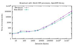
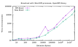
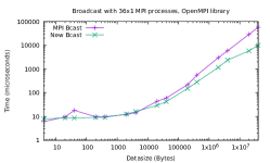
Figure 1: Broadcast results, native versus new, with the OpenMPI 4.1.4 library with $p=36\times 32,p=36\times 4,p=36\times 1$ MPI processes. The constant factor $F$ for the size of the blocks has been chosen as $F=70$. The MPI datatype is MPI_INT.

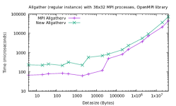
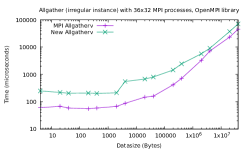
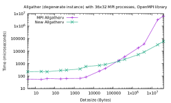
Figure 2: Irregular allgather results, native versus new, with the OpenMPI 4.1.4 library with $p=36\times 32$ MPI processes and different types of input problems (regular, irregular, degenerate). The constant factor $G$ for the number of blocks has been chosen as $G=40$. The MPI datatype is MPI_INT.

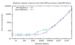
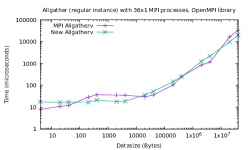
Figure 3: Regular allgather results, native versus new, with the OpenMPI 4.1.4 library with $p=36\times 32,p=36\times 4,p=36\times 1$ MPI processes. The constant factor $G$ for the number of blocks has been chosen as $G=40$. The MPI datatype is MPI_INT.

The results for MPI_Bcast are shown in Figure 1 for the full $36$ nodes of the system and different number of MPI processes per node, namely $32,4$ and $1$. It is noteworthy that the new implementation which assumes homogeneous communication can be significantly faster than the OpenMPI 4.1.4 baseline library implementation even for the $36\times 32$ process case.

The results for MPI_Allgatherv are shown in Figure 2 for $p=36\times 32$ MPI processes and different types of input problems. The regular problem divides the given input size $m$ roughly evenly over the processes in chunks of $m/p$ elements. The irregular problem divides the input in chunks of size roughly $(i\bmod 3)m/p$ for process $i=0,1,\ldots,p-1$. The degenerate problem has one process contribute the full input of size $m$ and all other process no input elements. For the degenerate problem, the performance of the OpenMPI 4.1.4 baseline library indeed degenerates and is a factor of close to 100 slower than the new implementation, where the running time is largely independent of the problem type. The running time of the new MPI_Allgatherv implementation is in the ballpark of MPI_Bcast for the same total problem size. For completeness, Figure 3 gives the running times for the regular problems with fewer MPI processes per node, $p=36\times 4$ and $p=36\times 1$.

4 Summary

We showed that round-optimal broadcast schedules on fully connected, one-ported, fully bidirectional $p$-processor systems can indeed be computed in $O(\log p)$ time steps per processor. This affirmatively answers the long standing open questions posed in [12, 10, 8, 9]. We repeated experiments indicating that the computations are feasible for use in practical implementations of MPI_Bcast and MPI_Allgatherv. A more careful evaluation of these implementations, also in versions that are more suitable to systems with hierarchical, non-homogeneous communication systems is ongoing and should be found elsewhere.

For the full $O(\log p)$-sized schedule computations an overhead of $O(\log p)$ is incurred, but complexity per neighboring processor is only $O(1)$ amortized. Would it be possible to find each send and receive block in $O(1)$ worst-case time? Also interesting is to characterize when the schedules are unique, how many different schedules there are for a given $p$, and for which $\lceil\log_{2}p\rceil$-regular circulant graphs the constructions can work.

References

- [1] Amotz Bar-Noy and Shlomo Kipnis. Broadcasting multiple messages in simultaneous send/receive systems. Discrete Applied Mathematics, 55(2):95–105, 1994.
- [2] Amotz Bar-Noy, Shlomo Kipnis, and Baruch Schieber. Optimal multiple message broadcasting in telephone-like communication systems. Discrete Applied Mathematics, 100(1–2):1–15, 2000.
- [3] Bin Jia. Process cooperation in multiple message broadcast. Parallel Computing, 35(12):572–580, 2009.
- [4] S. Lennart Johnsson and Ching-Tien Ho. Optimum broadcasting and personalized communication in hypercubes. IEEE Transactions on Computers, 38(9):1249–1268, 1989.
- [5] Oh-Heum Kwon and Kyung-Yong Chwa. Multiple message broadcasting in communication networks. Networks, 26:253–261, 1995.
- [6] MPI Forum. MPI: A Message-Passing Interface Standard. Version 4.0, June 9th 2021. www.mpi-forum.org.
- [7] Hubert Ritzdorf and Jesper Larsson Träff. Collective operations in NEC’s high-performance MPI libraries. In 20th International Parallel and Distributed Processing Symposium (IPDPS), page 100, 2006.
- [8] Jesper Larsson Träff. Brief announcement: Fast(er) construction of round-optimal -block broadcast schedules. In 34th ACM Symposium on Parallelism in Algorithms and Architectures (SPAA), pages 143–146. ACM, 2022.
- [9] Jesper Larsson Träff. Fast(er) construction of round-optimal -block broadcast schedules. In IEEE International Conference on Cluster Computing (CLUSTER), pages 142–151. IEEE Computer Society, 2022.
- [10] Jesper Larsson Träff. (Poly)logarithmic time construction of round-optimal -block broadcast schedules for broadcast and irregular allgather in MPI. arXiv:2205.10072, 2022.
- [11] Jesper Larsson Träff and Sascha Hunold. Decomposing MPI collectives for exploiting multi-lane communication. In IEEE International Conference on Cluster Computing (CLUSTER), pages 270–280. IEEE Computer Society, 2020.
- [12] Jesper Larsson Träff and Andreas Ripke. Optimal broadcast for fully connected processor-node networks. Journal of Parallel and Distributed Computing, 68(7):887–901, 2008.