Suppression of polaron self-localization by correlations

Abstract

We investigate self-localization of a polaron in a homogeneous Bose-Einstein condensate in one dimension. This effect, where an impurity is trapped by the deformation that it causes in the surrounding Bose gas, has been first predicted by mean field calculations, but has not been seen in experiments. We study the system in one dimension, where, according to the mean field approximation, the self-localization effect is particularly robust, and present for arbitrarily weak impurity-boson interactions. We address the question whether self-localization is a real effect by developing a variational method which incorporates impurity-boson correlations non-perturbatively and solving the resulting inhomogeneous correlated polaron equations. We find that correlations inhibit self-localization except for very strongly repulsive or attractive impurity-boson interactions. Our prediction for the critical interaction strength for self-localization agrees with a sharp drop of the inverse effective mass to almost zero found in quantum Monte Carlo simulations of polarons in one dimension.

I Introduction

The original Bose polaron problem concerns an electron in a solid which is dressed by small distortions of the crystal lattice and was modelled by Fröhlich Fröhlich (1954). Another type of polaron is formed by an electron or impurity atom in superfluid ⁴He. This problem has long been studiedTabbert et al. (1997) and later extended to molecular impurities and impurity aggregates in ⁴He, which lead to a new type of low-temperature spectroscopy of molecules Toennies and Vilesov (2004); Toennies (2022). More recently, polarons of mobile impurities have been experimentally realized in ultracold Bose gasesCatani et al. (2012); Hu et al. (2016); Jørgensen et al. (2016).

For electrons in ionic solids Landau (1933) and also in superfluid ⁴He Jortner et al. (1965) a mechanism for self-localization, or self-trapping, was proposedEmin (2013). Self-localization implies that, even in the absence of an external trap potential, the impurity probability density $\rho({\bf r}_{0})$ is not uniform but trapped by the distortion of the density of phonons or He atoms created by the impurity itself. In Refs.  Cucchietti and Timmermans, 2006; Kalas and Blume, 2006 based on the mean field (MF) approach self-localization has also been predicted for polarons in a Bose-Einstein condensate. According to Cuccietti et al.Cucchietti and Timmermans (2006) a polaron in a three-dimensional homogeneous Bose gas self-localizes above a critical impurity-boson interaction strength, while below it the polaron ground state is homogeneous. This would imply a phase transition to a translation symmetry breaking ground state. Subsequently, other works have also predicted this effect, e.g. for neutral polarons, again using the MF approximation Sacha and Timmermans (2006); Bruderer et al. (2008); Santamore and Timmermans (2011); Blinova et al. (2013); Li et al. (2013), including finite temperature Boudjemâa (2014), and also with other methods such as path integrals Tempere et al. (2009); Novikov and Ovchinnikov (2010). Also ionic polarons Casteels et al. (2011) and angular polarons Li et al. (2017) have been predicted to self-localize. However, other works have not seen evidence of self-localization in three dimensions Li and Das Sarma (2014); Ardila and Giorgini (2015); Hahn et al. (2018), nor has it been observed experimentally. This raises the question whether self-localization is a methodological artifact or a real effect.

In one dimension the MF approximation predicts a self-trapped polaron regardless of the strength of the impurity-boson interactionBruderer et al. (2008). Exact quantum Monte Carlo simulations Parisi and Giorgini (2017) indeed predict an essentially divergent polaron effective mass above a certain impurity-boson interaction strength, i.e. the polaron becomes immobile, which would be consistent with self-localization for strong interactions. Conversely, Ref. Grusdt et al., 2017 found a finite effective mass for attractive impurity-boson interaction, using the same Monte Carlo method for similar boson-boson interaction strengths but smaller mass ratio. Indirect measurements of Bose polarons in one dimension gave an even lower effective mass Catani et al. (2012).

The goal of this work is to check if the self-localized ground state predicted by the MF approximation is a real effect or an artifact of the uncorrelated Hartree ansatz of MF. To check this, we take a crucial step beyond the Hartree ansatz by incorporating impurity-boson correlations in a non-perturbative way, while treating the weakly interacting Bose background still in the MF approximation, thus omitting boson-boson correlations. We note that the perturbative treatment of correlations (then usually referred to as quantum fluctuations) has been shown to lead to corrections to the density $\rho(x_{0})$ of a self-localized impurity in one dimension Sacha and Timmermans (2006) but still preserves self-localization. In this work we show that with a non-perturbative treatment of impurity-boson correlations impurity self-localization happens only for very strongly attractive or repulsive impurity-boson interactions.

II Theory and Method

The Hamiltonian of one impurity and $N$ bosons in one dimension is given by

$$H =-{\hbar^{2}\over 2M}{\partial^{2}\over\partial x_{0}^{2}}-{\hbar^{2}\over 2m}\sum_{i=1}^{N}{\partial^{2}\over\partial x_{i}^{2}}+\sum_{i=1}^{N}U(x_{0}-x_{i})$$

$$+\lambda_{\text{BB}}\sum_{i<j}\delta(x_{i}-x_{j})$$ (1)

consisting of the kinetic energy of the impurity, the kinetic energy of the bosons, the impurity-boson interaction and the boson-boson interaction. The boson-boson interaction is modelled by a contact potential with strength $\lambda_{\text{BB}}$, which is related to the scattering length $a_{\text{BB}}$ by $\lambda_{\text{BB}}=\frac{-2\hbar^{2}}{a_{\text{BB}}m}$ Bloch (1973); Pitaevskii and Stringari (2003). The impurity-boson interaction is modelled by a finite range potential, for which we choose a Gaussian, $U(x)={U_{0}\over 2\sigma_{U}^{2}}\exp\left[-{x^{2}\over\sigma_{U}^{2}}\right]$, characterized by the strength and width parameters $U_{0}$ and $\sigma_{U}$.

The MF approach is usually derived in a variational formulation, with the Hartree ansatz wave function for one impurity in a bath of $N$ bosons:

$$\Psi_{\rm MF}=\eta(x_{0})\prod\limits_{i=1}^{N}\psi(x_{i}).$$ (2)

This wave function does not account for the correlations caused by the interactions, e.g. the decrease of the probability $|\Psi(x_{0},\dots,x_{i},\dots)|^{2}$ if a boson at $x_{i}$ is close to a repulsive impurity at $x_{0}$. The optimization of $\Psi_{\rm MF}$ leads to one-body equations with effective potentials, the “mean fields”. The uncorrelated MF ansatz (2) can be expected to be a poor approximation of the true many-body wave function if impurity-boson interactions are strong (but our results show it is a poor approximation for weak interaction as well). Therefore, we generalize the ansatz by replacing the boson one-body functions $\psi(x_{i})$ with impurity-boson pair correlation functions $f(x_{0},x_{i})$:

$$\Psi={1\over\Omega^{N/2}}\eta(x_{0})\prod\limits_{i=1}^{N}f(x_{0},x_{i}),$$ (3)

where it turns out to be convenient to introduce a prefactor including the normalization volume $\Omega$. This is a Jastrow-Feenberg ansatz wave function Feenberg (1969) but limited to impurity-boson correlations. We refer to it as the inhomogeneous correlated polaron (inh-CP) ansatz.

If the ground state is assumed homogeneous, i.e. translationally invariant like the Hamiltonian, the ansatz (3) simplifies to

$$\Psi_{\text{hom}}={1\over\Omega^{(N+1)/2}}\prod\limits_{i=1}^{N}f_{\text{hom}}(x_{0}-x_{i}),$$ (4)

which was studied already by Gross Gross (1962). Of course, we cannot make this assumption of translational invariance if we want to study the possible symmetry breaking by self-localization of the impurity. But the homogeneous correlated polaron (hom-CP) ansatz (4) will still be useful: if self-localization is indeed energetically favorable, the energy difference between the inh-CP and the hom-CP result is the energy gained by forming a self-localized ground state.

Our ansatz (3) includes impurity-boson correlations but still treats the (weakly interacting) Bose background in the MF approximation, as it does not include boson-boson correlations. Since we take only one step beyond the MF approach, this allows for a comprehensible comparison between our method and the MF approach. Impurities immersed in a strongly interacting Bose liquid like ⁴He, however, require the inclusion of boson-boson correlations. Optimizing such a full Jastrow-Feenberg ansatz leads to the hypernetted-chain Euler-Lagrange methodKrotscheck (2002); Polls and Mazzanti (2002). The method and its time-dependent generalization have been used extensively to study impurities in ⁴He Krotscheck and Saarela (1993); Krotscheck et al. (1998); Zillich and Whaley (2010).

Before deriving equations for $\eta(x_{0})$ and $f(x_{0},x_{i})$ from the Ritz’ variational principle, we need an expression for the energy functional $E=\langle\Psi|H|\Psi\rangle$, where we assume normalization of the wave function, $\langle\Psi|\Psi\rangle=1$. The 4 terms in the Hamiltonian (1) lead to the following 4 terms in $E$:

$$E =\frac{\hbar^{2}}{2M}\int\!\mathrm{d}\mathbf{x}\,\left({\partial\Psi\over\partial x_{0}}\right)^{2}$$

$$+N\frac{\hbar^{2}}{2m}\int\!\mathrm{d}\mathbf{x}\,\left({\partial\Psi\over\partial x_{1}}\right)^{2}+N\int\!\mathrm{d}\mathbf{x}\ \Psi^{2}\ U(x_{0}-x_{1})$$

$$+\frac{N(N-1)}{2}\int\!\mathrm{d}\mathbf{x}\ \Psi^{2}\ \lambda_{\text{BB}}\ \delta(x_{1}-x_{2}),$$ (5)

where $\mathrm{d}\mathbf{x}=dx_{0}\,dx_{1}\,...\,dx_{N}$, and $\Psi$ is the correlated polaron ansatz (3). Owing to the star-shaped correlation structure, where the impurity is correlated with all bosons but the bosons are not correlated between themselves, most of the $N+1$ integrals in $E$ factorize and yield $\int dx_{1}^{\prime}\,f(x_{0},x_{1}^{\prime})^{2}$. We abbreviate this partially integrated correlation function

$$\bar{f}(x_{0})\equiv\Omega^{-1}\!\int dx_{1}^{\prime}\ f(x_{0},x_{1}^{\prime})^{2}.$$ (6)

We obtain the energy functional

$$E\ = \ \frac{\hbar^{2}}{2M}\ \Biggl{\{}\int\!dx_{0}\,\left(\frac{\partial\eta(x_{0})}{\partial x_{0}}\right)^{2}\bar{f}(x_{0})^{N}-\frac{N}{\Omega}\int\!dx_{0}dx_{1}\,\eta(x_{0})^{2}\,\bar{f}(x_{0})^{N-1}f(x_{0},x_{1})\,\frac{\partial^{2}f(x_{0},x_{1})}{\partial x_{0}^{2}}$$

$$\hskip 29.87547pt-\frac{N(N-1)}{\Omega^{2}}\int\!dx_{0}\,\eta(x_{0})^{2}\,\bar{f}(x_{0})^{N-2}\left[\int\!dx_{1}\,f(x_{0},x_{1})\,\frac{\partial f(x_{0},x_{1})}{\partial x_{0}}\right]^{2}\Biggr{\}}$$

$$+\frac{\hbar^{2}}{2m}\frac{N}{\Omega}\int\!dx_{0}dx_{1}\,\eta(x_{0})^{2}\,\bar{f}(x_{0})^{N-1}\left(\frac{\partial f(x_{0},x_{1})}{\partial x_{1}}\right)^{2}+\frac{N}{\Omega}\int\!dx_{0}dx_{1}\,\eta(x_{0})^{2}\,\bar{f}(x_{0})^{N-1}\,f(x_{0},x_{1})^{2}\,U(x_{0},x_{1})$$

$$+\frac{\lambda_{\text{BB}}}{2}\ \frac{N(N-1)}{\Omega^{2}}\int\!dx_{0}dx_{1}\,\eta(x_{0})^{2}\,\bar{f}(x_{0})^{N-2}\,f(x_{0},x_{1})^{4}.$$ (7)

In a study of self-localization, we are primarily interested in the impurity density $\rho_{\text{I}}(x_{0})$. Without an external trapping potential, the impurity density is constant in the absence of self-localization, $\rho_{\text{I}}(x_{0})={1\over\Omega}$, while in the presence of self-localization $\rho_{\text{I}}(x_{0})$ peaks at a random location $\bar{x}_{0}$ and falls to zero away from $\bar{x}_{0}$. Similarly, the density of the Bose gas $\rho_{\text{B}}(x_{1})$ is constant in the first case, $\rho_{\text{B}}(x_{1})={N\over\Omega}$ , while it has a valley/peak for repulsive/attractive impurity-boson interaction in the latter case. For the correlated polaron ansatz (3), the impurity density is given by

$$\rho_{\text{I}}(x_{0})=\int\!dx_{1}\dots dx_{N}|\Psi|^{2}=\eta(x_{0})^{2}\bar{f}(x_{0})^{N},$$ (8)

and the boson density is given by

$$\rho_{\text{B}}(x_{1}) =N\int\!dx_{0}dx_{2}\dots dx_{N}|\Psi|^{2}$$

$$={N\over\Omega}\int\!dx_{0}\ \eta(x_{0})^{2}\bar{f}(x_{0})^{N-1}f(x_{0},x_{1})^{2},$$ (9)

where normalization of the wave function was assumed.

According to the Ritz’ variational principle the optimal $\eta(x_{0})$ and $f(x_{0},x_{1})$ are obtained from minimizing the energy (7), i.e. setting its functional derivatives with respect to $\eta(x_{0})$ and $f(x_{0},x_{1})$ to zero. To ensure normalization of the wave function we introduce a Lagrange multiplier $\lambda$. Hence, we need to optimize the Lagrangian

$$L=E+\lambda\left\{1-\int dx_{0}\ \eta(x_{0})^{2}\ \bar{f}(x_{0})^{N}\right\}.$$ (10)

The inh-CP equations for the general inhomogeneous case are the coupled Euler-Lagrange equations, formally written as

$$\hskip 8.5359pt\frac{\delta L}{\delta\eta(x_{0})}=0,$$ (11)

$$\frac{\delta L}{\delta f(x_{0},x_{1})}=0.$$ (12)

Their explicit form is derived in appendix A, where we show that in the thermodynamic limit $N\to\infty$ and $\Omega\to\infty$ with $\rho={N\over\Omega}$ fixed, we obtain a 1-body equation for the square root of the impurity density $g(x_{0})=\sqrt{\rho_{\text{I}}(x_{0})}$ and a two-body equation for $\tilde{f}(x_{0},x_{1})\equiv g(x_{0})f(x_{0},x_{1})$:

$$\mu_{\text{I}}\ g(x_{0})= -\frac{\hbar^{2}}{2M}\ \frac{\partial^{2}g(x_{0})}{\partial x_{0}^{2}}+V_{g}(x_{0})\,g(x_{0})$$ (13)

$$\mu_{\text{B}}\ \tilde{f}(x_{0},x_{1})= -\frac{\hbar^{2}}{2M}\frac{\partial^{2}\tilde{f}(x_{0},x_{1})}{\partial{x_{0}}^{2}}-\frac{\hbar^{2}}{2m}\frac{\partial^{2}\tilde{f}(x_{0},x_{1})}{\partial{x_{1}}^{2}}+V_{f}(x_{0},x_{1})\,\tilde{f}(x_{0},x_{1})$$ (14)

with the impurity and boson chemical potential $\mu_{\text{I}}$ and $\mu_{\text{B}}$ and the effective one-body and two-body potentials

$$V_{g}(x_{0}) =\frac{\hbar^{2}}{2M}\rho\int\!dx_{1}^{\prime}\left(\frac{\partial f(x_{0},x_{1}^{\prime})}{\partial x_{0}}\right)^{2}+\frac{\hbar^{2}}{2m}\rho\int\!dx_{1}^{\prime}\left(\frac{\partial f(x_{0},x_{1}^{\prime})}{\partial x_{1}^{\prime}}\right)^{2}+\rho\int\!dx_{1}^{\prime}\,f(x_{0},x_{1}^{\prime})^{2}\,U(x_{0},x_{1}^{\prime})$$

$$+\lambda_{\text{BB}}\frac{\rho^{2}}{2}\int\!dx_{1}^{\prime}\,\Bigl{(}f(x_{0},x_{1}^{\prime})^{4}-2\ f(x_{0},x_{1}^{\prime})^{2}+1\Bigr{)}$$ (15)

$$V_{f}(x_{0},x_{1}) =\frac{\hbar^{2}}{2M}\frac{1}{g(x_{0})}\frac{\partial^{2}g(x_{0})}{\partial x_{0}^{2}}+U(x_{0},x_{1})+\lambda_{\text{BB}}\rho\ \frac{\tilde{f}(x_{0},x_{1})^{2}}{g(x_{0})^{2}}.$$ (16)

We have cast the two coupled inh-CP equations into the form of a one- and a two-body nonlinear Schrödinger equation, respectively, with effective potentials (15) and (16) that depend on $g(x_{0})$ and $\tilde{f}(x_{0},x_{1})$ itself. Similarly to other nonlinear Schrödinger equationsChin and Krotscheck (2005), Eqns. (13) and (14) can be solved self-consistently by imaginary time propagation, where we always start the propagation with self-localized trial states, for example the MF ground state. Details are given in appendix B.

III Results

We present results for the Bose polaron ground state in one dimension for three levels of approximation:

1. solving the full inh-CP equations (13) and (14), derived in this work and based on the ansatz (3);

2. solving the special case of the hom-CP equation, derived in Ref. Gross, 1962, based on the ansatz (4), that precludes self-localization;

3. solving the MF equations, based on the ansatz (2), which according to Ref. Bruderer et al., 2008 always result in self-localization in one dimension.

In all three types of calculations, we use the same Gaussian interaction model. Following Bruderer et al.Bruderer et al. (2008), we measure length in units of the healing length $\xi=\hbar/\sqrt{\lambda_{\text{BB}}\rho m}$ and energy in units of $E_{0}=\lambda_{\text{BB}}\rho$. This leaves us with three dimensionless essential parameters characterizing the Bose polaron system (1): the mass ratio $\alpha=m/M$, the relative interaction strength $\beta=\lambda_{\text{IB}}/\lambda_{\text{BB}}$ and a density parameter $\gamma=1/(\rho\xi)$. $\lambda_{\text{IB}}$ is obtained from the scattering length $a_{\text{IB}}$ via $\lambda_{\text{IB}}=-\hbar/a_{\text{IB}}(1/M+1/m)$, and the scattering length $a_{\text{IB}}$ is obtained from the parameters $U_{0}$ and $\sigma_{U}$ the Gaussian model interaction using the results of Ref. Jeszenszki et al., 2018. We have confirmed the universality of the interaction model, i.e. that our results depend only on $\lambda_{\text{IB}}$ and not on the parameters $U_{0}$ and $\sigma_{U}$ if $\sigma_{U}$ is chosen very small. Too small values for $\sigma_{U}$ would require a very fine discretization and correspondingly high numerical effort. Therefore, we choose $\sigma_{U}=0.1$, where results differ only insignificantly from the universal limit.

We compare results obtained with the inh-CP and the hom-CP equations to ensure numerical consistency, and also to calculate the formation energy (called binding energy in Ref. Cucchietti and Timmermans, 2006) gained from self-localization if we do find self-localized polarons. But the main goal of this work is to compare the inh-CP results and MF results, i.e. results with and without including correlations, to see whether self-localization still occurs when impurity-boson correlations are included in the variational ansatz. We note that both solving the hom-CP equation and solving the MF equations is numerically straightforward and fast since all quantities depend on a single coordinate, unlike $f(x_{0},x_{1})$ in the inh-CP ansatz (3).

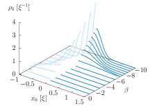
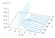
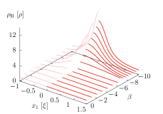
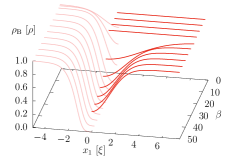
Figure 1: The impurity density $\rho_{\text{I}}(x_{0})$ (top panels) and boson density $\rho_{\text{B}}(x_{1})$ (bottom panels) are shown as functions of $\beta$. The correlated polaron results are depicted on the positive side of the coordinate axis $x_{0}$ or $x_{1}$, while the mean field results are depicted on the negative side. The left and right panels show results for attractive and repulsive impurity-boson interactions, respectively. A constant $\rho_{\text{I}}(x_{0})$ and $\rho_{\text{B}}(x_{1})$ means there is no self-localization for the corresponding value of $\beta$. All results are for $\gamma=0.5$.

In this work we restrict ourselves to equal impurity and boson mass, i.e. $\alpha=1$. The parameter $\gamma$ is related to the gas parameter, $\rho|a_{\text{BB}}|=2/\gamma^{2}$. A small parameter $\gamma$ signifies weak boson-boson interactions (i.e. large $|a_{\text{BB}}|$) and/or high density, while $\gamma\to\infty$ is the strongly correlated Tonks-Girardeau limit Girardeau (1960). We study two cases, $\gamma=0.2$ and $\gamma=0.5$, which both correspond to a weakly interacting Bose gas, where it may be justified to neglect boson-boson correlations as done in the ansatz (3). We vary the relative impurity-boson interaction strength $\beta$ over a wide range from strongly attractive to strongly repulsive.

III.1 Density and localization length

In Fig. 1 we show the impurity density $\rho_{\text{I}}(x_{0})$ (top panels) and the boson density $\rho_{\text{B}}(x_{1})$ (bottom panels) for attractive impurity-boson interactions, $-10\leq\beta<0$, (left panels) and repulsive interaction $0<\beta\leq 50$ (right panels). We show only half of the densities since they are assumed to be symmetric. The darker lines (positive coordinates) are the solutions of the inh-CP equations, while the lighter lines (negative coordinates) are the solutions of the MF equations, calculated also in Ref. Bruderer et al., 2008. All calculations in Fig. 1 are done for $\gamma=0.5$.

The comparison in Fig. 1 demonstrates that incorporating the impurity-boson correlations strongly reduces the tendency towards self-localization. The MF approximation predicts that the polaron self-localizes for all values of $\beta$, where $\rho_{\text{I}}(x_{0})$ and $\rho_{\text{B}}(x_{1})$ becomes narrower for larger $|\beta|$.Bruderer et al. (2008) Conversely, the ground state of the correlated polaron is qualitatively and quantitatively quite different: for a wide $\beta$-range the polaron does not self-localize at all, thus $\rho_{\text{I}}(x_{0})$ and $\rho_{\text{B}}(x_{1})$ are simply constant. It may come as a surprise that especially for weak interactions the MF approximation gives a wrong result regarding the question of self-localization, which demonstrates that in one dimension correlations should never be neglected. Only for sufficiently strong attraction or repulsion, the correlated polaron self-localizes, but both $\rho_{\text{I}}(x_{0})$ and $\rho_{\text{B}}(x_{1})$ are significantly broader than in the MF approximation.

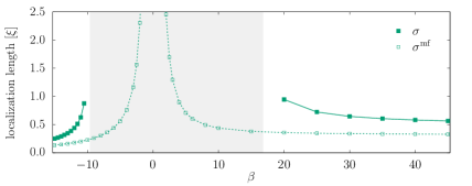
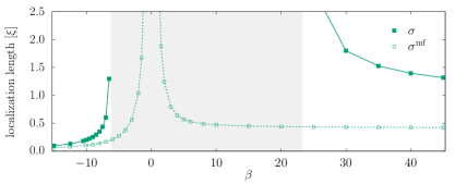
Figure 2: The localization length $\sigma$ of a polaron is plotted as a function of $\beta$ for $\gamma=0.2$ (top panel) and 0.5 (bottom panel). The filled and open symbols are the correlated and mean field results, respectively, the latter agreeing with Ref. Bruderer et al., 2008. The shaded area indicates the range of $\beta$ where no self-localization occurs according to our correlated results.

A localized polaron can be characterized by a localization length $\sigma$, e.g. by fitting a Gaussian $\exp[-x_{0}^{2}/(2\sigma^{2})]/(\sigma\sqrt{2\pi})$ to the impurity densities $\rho_{\text{I}}(x_{0})$ shown in Fig. 1. $\sigma\to\infty$ means the polaron delocalizes. In Fig. 2 we show the localization length $\sigma$ of the correlated polaron (filled squares) and the corresponding $\sigma^{\text{mf}}$ of the MF polaron (open squares) as functions of the relative interaction strength $\beta$ for $\gamma=0.2$ (top) and $\gamma=0.5$ (bottom). Since in all our calculations, including the MF calculations, we use a Gaussian interaction of finite width $\sigma_{U}=0.1$ instead of a contact potential, our results for $\sigma^{\text{mf}}$ deviate slightly from Ref. Bruderer et al., 2008, at most by 10%. Since the MF approximation predicts unconditional self-localization in 1D, $\sigma^{\text{mf}}$ is finite for all $\beta\neq 0$. For the correlated polaron, we get a large range of $\beta$ where the polaron is delocalized, indicated by the grey area. Therefore, $\sigma$ is not only significantly larger than $\sigma^{\text{mf}}$, but it diverges at a critical attractive and repulsive relative interaction strength $\beta_{\text{cr,1}}$ and $\beta_{\text{cr,2}}$, respectively, the value of which depends on $\gamma$. Since a large $\sigma$ requires a large computational domain, approaching the critical $\beta$ becomes numerically expensive and we estimate it by fitting to $a_{1}|\beta-\beta_{\text{cr,1}}|^{c_{1}}$ for the attractive side and $a_{2}|1-\beta_{\text{cr,1}}/\beta|^{c_{2}}$ for the repulsive side (where $\sigma$ seems to saturate at a finite value for large $\beta$). The estimates are tabulated in Tab. 1.

$\gamma$	$\beta_{\text{cr,1}}$	$\beta_{\text{cr,2}}$	$\gamma_{\text{P}}$	$\eta_{\text{cr,2}}$	$\eta_{\text{cr,2}}$
0.2	-9.6	16.8	0.04	-0.38	0.67
0.5	-6.2	23.3	0.25	-1.55	5.82

Table 1: The critical relative interaction strengths $\beta_{\text{cr,1/2}}$ for self-localization, obtained from solving the inh-CP equations. We also tabulate the results expressed in alternative dimensionless units (see text) for better comparison with Ref. Parisi and Giorgini, 2017.

The Bose polaron in one dimension was studied with diffusion Monte Carlo simulations Parisi and Giorgini (2017); Grusdt et al. (2017). The trial wave functions used in that work are translationally invariant, which may mask a self-localization effect. Nonetheless, a relatively sharp increase of the polaron effective mass to a very large value was observed on both the attractive and repulsive side. Parisi et al. Parisi and Giorgini (2017) considered equal masses for impurity and bosons, which allows comparison with the present work. They use the parameters $\gamma_{\text{P}}=\gamma^{2}$ and $\eta=\beta\gamma^{2}$ to characterize boson density/interactions and impurity-boson interactions, respectively. For better comparison Tab. 1 provides the critical interaction strength also in terms of $\gamma_{\text{P}}$ and $\eta$. The closest values of $\gamma_{\text{P}}$ compared to our values are $\gamma^{\text{(MC)}}_{\text{P}}=0.02$ and 0.2. Fig. 4 in Ref. Parisi and Giorgini, 2017 shows that for $\gamma^{\text{(MC)}}_{\text{P}}=0.02$ the inverse effective mass essentially vanishes for $\eta\approx-1$ and for $\eta\approx 1$ for attractive and repulsive interactions, respectively; for $\gamma^{\text{(MC)}}_{\text{P}}=0.2$ the corresponding values are $\eta\approx-2$ and $\eta\approx 10$, however the statistical fluctuations and the logarithmic scale makes it hard to give precise numbers. Considering this uncertainty and our slightly different values for $\gamma_{\text{P}}$, our prediction for the critical interaction strength for a self-localized polaron ground state is consistent with that for an essentially infinite effective mass obtained with diffusion Monte Carlo.

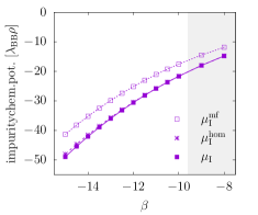
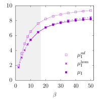
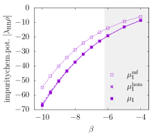
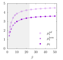
Figure 3: The impurity chemical potential $\mu_{\text{I}}$ (filled squares) from the solution of the inhomogeneous correlated polaron equations is plotted as a function of $\beta$ for $\gamma=0.2$ (top panels) and 0.5 (bottom panels), together with the mean field prediction $\mu_{\text{I}}^{\text{mf}}$ (open squares) and the homogeneous correlated polaron prediction $\mu_{\text{I}}^{\text{hom}}$ (stars). Left and right panels show attractive and repulsive impurity-boson interactions, respectively.

III.2 Chemical potential

Solving the correlated polaron equations (13) and (14) yields not only $g(x_{0})$ and $\tilde{f}(x_{0},x_{1})$ but also the impurity and boson chemical potentials $\mu_{\text{I}}$ and $\mu_{\text{B}}$. For the latter we obtain the trivial result $\mu_{\text{B}}/E_{0}=1$, i.e. the MF approximation of the pure Bose gas, which is not altered by a single impurity in the thermodynamic limit. Slight numerical deviations from unity provide a measure of finite size effects.

The impurity chemical potential $\mu_{\text{I}}$ provides nontrivial information. According to the Ritz’ variational principle, better variational wave functions yield lower energies, closer to the exact ground state energy. This is also true for $\mu_{\text{I}}$, because it is obtained by subtracting the constant $E_{0,N}$ from the ground state energy, see appendix A. Hence, the chemical potential of the correlated impurity must be lower than that of the MF impurity, $\mu_{\text{I}}<\mu_{\text{I}}^{\text{mf}}$. In Fig. 3 we show $\mu_{\text{I}}$ and $\mu_{\text{I}}^{\text{mf}}$ as functions of $\beta$ for $\gamma=0.5$ (top panels) and 0.2 (bottom panels). For all cases, $\mu_{\text{I}}^{\text{mf}}$ is higher than $\mu_{\text{I}}$, as it should be. Furthermore, we expect $\mu_{\text{I}}<0$ for $\beta<0$ and vice versa, which is indeed the case for both $\mu_{\text{I}}$ and $\mu_{\text{I}}^{\text{mf}}$. For attractive impurity-boson interactions, shown in the left panels, $\mu_{\text{I}}$ shows no sign of saturating to a finite value when $\beta$ is decreased to stronger attraction, in fact the slope steepens. For repulsive interactions (right panels), $\mu_{\text{I}}$ does saturate with increasing $\beta$. This is consistent with the behavior of the localization length shown in Fig. 2 for negative and positive $\beta$.

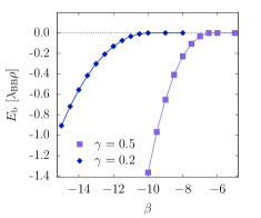
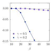
Figure 4: The formation energy $E_{b}=\mu_{\text{I}}-\mu_{\text{I}}^{\text{hom}}$ is plotted as a function of $\beta$, split into attractive and repulsive interaction (left and right panel). Self-localization happens only if $E_{b}<0$.

The comparison between $\mu_{\text{I}}$ and $\mu_{\text{I}}^{\text{mf}}$ serves mainly as a check that we did not converge to an unphysical local energy minimum. More interesting is the comparison of the chemical potentials obtained from the inhomogeneous and the homogeneous polaron equations, $\mu_{\text{I}}$ and $\mu_{\text{I}}^{\text{hom}}$, respectively, because the difference is the formation energy of self-localization, $E_{b}=\mu_{\text{I}}-\mu_{\text{I}}^{\text{hom}}$, i.e. the energy gained by localization. $\mu_{\text{I}}^{\text{hom}}$ is shown in Fig. 3 together with $\mu_{\text{I}}$ and $\mu_{\text{I}}^{\text{mf}}$, but the difference between $\mu_{\text{I}}$ and $\mu_{\text{I}}^{\text{hom}}$ is barely visible. In Fig. 4 we show the formation energy $E_{b}$, which is about two orders of magnitude smaller than $\mu_{\text{I}}$, and its determination without numerical bias is challenging. We note that the smallness of $E_{b}$ relative to $\mu_{\text{I}}$ would render its calculation by Monte Carlo simulation a formidable task.

If $\mu_{\text{I}}=\mu_{\text{I}}^{\text{hom}}$, thus $E_{b}=0$, no energy is gained from self-localization, which therefore does not happen. Indeed, in these cases the inh-CP solver converges to a constant polaron density, $\rho_{\text{I}}=1/\Omega$, with the same correlation function $f(x_{0},x_{1})$ as that of the hom-CP solution, $f^{\text{hom}}(x_{0}-x_{1})$. If $\mu_{\text{I}}<\mu_{\text{I}}^{\text{hom}}$, thus $E_{b}<0$, self-localization lowers the ground state with respect to a homogenous ground state. The critical relative interaction strength $\beta_{\text{cr,1}}$ and $\beta_{\text{cr,2}}$ discussed above is just the point where $E_{b}$ becomes 0.

We illustrate the difference between a homogeneous pair correlation $f(x_{0}-x_{1})$ of a delocalized ground state and the inhomogeneous pair correlation $f(x_{0},x_{1})$ of a self-localized ground state in Fig. 5 for $\gamma=0.5$. The left panel shows $f(x_{0},x_{1})$ for $\beta=-10$ (localized), which has only inversion symmetry. The right panel shows $f(x_{0},x_{1})=f^{\text{hom}}(x_{0}-x_{1})$ for $\beta=-5$ (homogeneous), which has translation symmetry with respect to the center of mass $(x_{0}+x_{1})/2$.

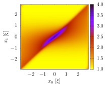
Figure 5: Optimal pair correlation $f(x_{0},x_{1})$ obtained from solving the inhomogeneous correlated polaron equations. For $\beta=-10$ (left panel) the polaron ground state is self-localized and for $\beta=-5$ (right panel) the ground state is homogeneous. The values at the upper left and lower right corners of the computational domain are a result of the periodic boundary conditions.

IV Conclusions

We revisited the self-localization problem of an impurity in a Bose gas, where the mean field (MF) approximation predicted self-localized polaron ground states in 3D,Cucchietti and Timmermans (2006), and later in 2D and 1D Bruderer et al. (2008); in particular in 1D, self-localization was predicted to happen for any strength of the impurity-boson interaction, quantified by the parameter $\beta$. Extending the MF method using the Bogoliubov method to account for quantum fluctuations has proven useful in many instances (dipolar interactions Lima and Pelster (2011), self-bound Bose mixturesPetrov (2015)), but is still only a perturbative expansion. In our work, we incorporate optimized, inhomogeneous impurity-boson correlations in a non-perturbative way and derive inhomogeneous correlated polaron (inh-CP) equations, which we solve numerically for the 1D case. The results of this improved variational ansatz for the ground state wave function shows that the MF approach is not sufficient to study polaron physics in 1D. Impurity-boson correlations suppress the tendency towards self-localization significantly, which happens only for strongly attractive or repulsive impurity-boson interactions. Despite being variational, our results are consistent with the sharp increase of the effective mass of the polaron at a similar critical impurity-boson interaction strength predicted by exact diffusion Monte Carlo simulations Parisi and Giorgini (2017).

In case of the MF approximation, it is straightforward to see why it might predict a spurious self-localization even for weak interactions: without correlations, i.e. using a Hartree ansatz (2), a localized impurity density and accordingly an inhomogeneous Bose density “mimics” the effect of a correlations as the most optimal solution of the Ritz’ variational problem. For example, for repulsive interactions the Bose density is suppressed around the localized impurity, lowering the total energy of a Hartree ansatz. Instead, in a correlated many-body wave function like (3), repulsion causes a correlation hole in the pair distribution function, which does not require self-localization of the polaron. Our method predicts self-localization only for strong impurity-boson interactions, but this is not a rigorous proof that such a breaking of the translational invariance of the Hamiltonian (1) is a real effect rather than a variational artifact. Further refinements beyond the variational wave function (3), such as boson-boson correlations or three body impurity-boson-boson correlations, may push the transition to self-localization to even stronger interactions. However, the above-mentioned consistency with exact Monte Carlo results lends credibility to the correlated polaron ansatz (3) in the regime of weak boson-boson interactions that we studied in this work.

Experimental observation of a possibly self-localized polaron is challenging. The smallness of the formation energy $E_{b}$ would require a low temperature, depending on the magnitude of $|\beta|$, where strongly attractive interactions, $\beta<0$, are clearly favorable according to our results. In higher dimensions, there is no evidence of a sharp increase of the effective mass of a polaron three dimensions, according to quantum Monte Carlo simulationsArdila and Giorgini (2015), but the MF approach Cucchietti and Timmermans (2006) does predict self-localization. Correlations tend to be less important in higher dimensions, and the MF approach usually becomes a better approximation. It will be interesting to see if there is a parameter regime where the correlated polaron ansatz (3) is self-localized in more than one dimension. Furthermore, the inh-CP method can be generalized to time-dependent problems, similarly to the time-dependent hypernetted-chain Euler-Lagrange method Gartner et al. (2023). This allows to calculate the effective mass but also to study nonequilibrium dynamics of polarons after a quench Grusdt et al. (2018), such as an interaction quench of $\beta$.

Our results pertain only to neutral atomic impurities. For dipolar and especially ionic impurities, which interact via long-ranged attractive potentials with the surrounding Bose gas due to induced dipoles, the situation may be different. Ions in BECs can dress themselves with a substantial cloud of bosons Astrakharchik et al. (2021), making ionic polarons a more likely candidate for self-localization.

Appendix A Derivation of the inhomogeneous correlated polaron equations

From the energy (7) and the resulting Lagrangian (10) we derive the inh-CP equations (13) and (14). The first Euler-Lagrange equation (11) becomes, after dividing by $2\bar{f}(x_{0})^{N}$,

$$\lambda\ \eta(x_{0})= -\frac{\hbar^{2}}{2M}\ \Biggl{\{}\frac{\partial^{2}\eta(x_{0})}{\partial x_{0}^{2}}+2\ \frac{N}{\Omega}\ \frac{\partial\eta(x_{0})}{\partial x_{0}}\,\frac{1}{\bar{f}(x_{0})}\int\!dx_{1}^{\prime}\,f(x_{0},x_{1}^{\prime})\,\frac{\partial f(x_{0},x_{1}^{\prime})}{\partial x_{0}}$$

$$\hskip 34.14322pt+\frac{N}{\Omega}\,\frac{\eta(x_{0})}{\bar{f}(x_{0})}\int\!dx_{1}^{\prime}\,f(x_{0},x_{1}^{\prime})\,\frac{\partial^{2}f(x_{0},x_{1}^{\prime})}{\partial x_{0}^{2}}+\frac{N(N-1)}{\Omega^{2}}\,\frac{\eta(x_{0})}{\bar{f}(x_{0})^{2}}\left[\int\!dx_{1}^{\prime}\,f(x_{0},x_{1}^{\prime})\,\frac{\partial f(x_{0},x_{1}^{\prime})}{\partial x_{0}}\right]^{2}\Biggr{\}}$$

$$+\frac{\hbar^{2}}{2m}\frac{N}{\Omega}\,\frac{\eta(x_{0})}{\bar{f}(x_{0})}\int\!dx_{1}^{\prime}\left(\frac{\partial f(x_{0},x_{1}^{\prime})}{\partial x_{1}^{\prime}}\right)^{2}+\frac{N}{\Omega}\,\frac{\eta(x_{0})}{\bar{f}(x_{0})}\int\!dx_{1}^{\prime}\,f(x_{0},x_{1}^{\prime})^{2}\ U(x_{0},x_{1}^{\prime})$$

$$+\frac{\lambda_{\text{BB}}}{2}\ \frac{N(N-1)}{\Omega^{2}}\frac{\eta(x_{0})}{\bar{f}(x_{0})^{2}}\int\,dx_{1}^{\prime}\,f(x_{0},x_{1}^{\prime})^{4}.$$ (17)

Note that, when we multiply this equation by $\eta(x_{0})\ \bar{f}(x_{0})^{N}$ and integrate over $x_{0}$, we obtain $\lambda=E$, i.e. the Lagrange multiplier is indeed the energy.

Using (7) and (10), the second Euler-Lagrange equation (11) becomes, after dividing by $\frac{2N}{\Omega}\bar{f}(x_{0})^{N-1}$,

$$E\ \eta(x_{0})^{2}\ f(x_{0},x_{1})=-\frac{\hbar^{2}}{2M}\ \Biggl{\{}\eta(x_{0})\ \frac{\partial^{2}\eta(x_{0})}{\partial x_{0}^{2}}\ f(x_{0},x_{1})+\eta(x_{0})^{2}\ \frac{\partial^{2}f(x_{0},x_{1})}{\partial x_{0}^{2}}$$

$$\hskip 36.98866pt+2\ \frac{N-1}{\Omega}\,\frac{\eta(x_{0})}{\bar{f}(x_{0})^{-1}}\,\frac{\partial\eta(x_{0})}{\partial x_{0}}\,f(x_{0},x_{1})\int\!dx_{1}^{\prime}\,f(x_{0},x_{1}^{\prime})\,\frac{\partial f(x_{0},x_{1}^{\prime})}{\partial x_{0}}$$

$$\hskip 36.98866pt+\frac{N-1}{\Omega}\,\frac{\eta(x_{0})^{2}}{\bar{f}(x_{0})}\,f(x_{0},x_{1})\int\!dx_{1}^{\prime}\,f(x_{0},x_{1}^{\prime})\ \frac{\partial^{2}f(x_{0},x_{1}^{\prime})}{\partial x_{0}^{2}}$$

$$\hskip 36.98866pt+\frac{(N-1)(N-2)}{\Omega^{2}}\frac{\eta(x_{0})^{2}}{\bar{f}(x_{0})^{2}}\,f(x_{0},x_{1})\left[\int\!dx_{1}^{\prime}\,f(x_{0},x_{1}^{\prime})\,\frac{\partial f(x_{0},x_{1}^{\prime})}{\partial x_{0}}\right]^{2}+2\ \eta(x_{0})\ \frac{\partial\eta(x_{0})}{\partial x_{0}}\ \frac{\partial f(x_{0},x_{1})}{\partial x_{0}}$$

$$\hskip 36.98866pt+2\ \frac{N-1}{\Omega}\frac{\eta(x_{0})^{2}}{\bar{f}(x_{0})}\,\frac{\partial f(x_{0},x_{1})}{\partial x_{0}}\int\!dx_{1}^{\prime}\,f(x_{0},x_{1}^{\prime})\,\frac{\partial f(x_{0},x_{1}^{\prime})}{\partial x_{0}}\Biggr{\}}$$

$$-\frac{\hbar^{2}}{2m}\,\Biggl{\{}\eta(x_{0})^{2}\,\frac{\partial^{2}f(x_{0},x_{1})}{\partial x_{1}^{2}}-\frac{N-1}{\Omega}\,\frac{\eta(x_{0})^{2}}{\bar{f}(x_{0})}\,f(x_{0},x_{1})\int\!dx_{1}^{\prime}\,\left(\frac{\partial f(x_{0},x_{1}^{\prime})}{\partial x_{1}^{\prime}}\right)^{2}\Biggr{\}}$$

$$+\eta(x_{0})^{2}\,f(x_{0},x_{1})\,U(x_{0},x_{1})+\frac{\eta(x_{0})^{2}}{\bar{f}(x_{0})}\,f(x_{0},x_{1})\int\!dx_{1}^{\prime}\,f(x_{0},x_{1}^{\prime})^{2}\,U(x_{0},x_{1}^{\prime})$$

$$+\lambda_{\text{BB}}\frac{N-1}{\Omega}\,\frac{eta(x_{0})^{2}}{\bar{f}(x_{0})}\,f(x_{0},x_{1})^{3}+\frac{\lambda_{\text{BB}}}{2}\frac{(N-1)(N-2)}{\Omega^{2}}\,\frac{\eta(x_{0})^{2}}{\bar{f}(x_{0})^{2}}\,f(x_{0},x_{1})\int\!dx_{1}^{\prime}\,f(x_{0},x_{1}^{\prime})^{4}.$$ (18)

We can simplify this lengthy equation by dividing by $\eta(x_{0})$ and subtracting eq. (17) multiplied by $f(x_{0},x_{1})$,

$$\Delta E\,\eta(x_{0})\,f(x_{0},x_{1})= -\frac{\hbar^{2}}{2M}\,\Biggl{\{}2\,\frac{\partial\eta(x_{0})}{\partial x_{0}}\,\frac{\partial f(x_{0},x_{1})}{\partial x_{0}}+2\frac{N-1}{\Omega}\,\frac{\eta(x_{0})}{\bar{f}(x_{0})}\,\frac{\partial f(x_{0},x_{1})}{\partial x_{0}}\int\!dx_{1}^{\prime}\,f(x_{0},x_{1}^{\prime})\,\frac{\partial f(x_{0},x_{1}^{\prime})}{\partial x_{0}}$$

$$\hskip 36.98866pt+\eta(x_{0})\ \frac{\partial^{2}f(x_{0},x_{1})}{\partial x_{0}^{2}}\Biggr{\}}$$

$$-\frac{\hbar^{2}}{2m}\,\eta(x_{0})\,\frac{\partial^{2}f(x_{0},x_{1})}{\partial x_{1}^{2}}\ +\ \eta(x_{0})\ U(x_{0},x_{1})\ f(x_{0},x_{1})$$

$$+\lambda_{\text{BB}}\frac{N-1}{\Omega}\,\frac{\eta(x_{0})}{\bar{f}(x_{0})}\,f(x_{0},x_{1})^{2}\,f(x_{0},x_{1}),$$ (19)

where we abbreviate

$$\Delta E\equiv -\frac{\hbar^{2}}{2M}\,\Biggl{\{}\frac{2}{\Omega}\,\frac{\partial\eta(x_{0})}{\partial x_{0}}\,\frac{1}{\bar{f}(x_{0})}\int\!dx_{1}^{\prime}\,f(x_{0},x_{1}^{\prime})\,\frac{\partial f(x_{0},x_{1}^{\prime})}{\partial x_{0}}+\frac{1}{\Omega}\,\frac{\eta(x_{0})}{\bar{f}(x_{0})}\int\!dx_{1}^{\prime}\,f(x_{0},x_{1}^{\prime})\,\frac{\partial^{2}f(x_{0},x_{1}^{\prime})}{\partial x_{0}^{2}}$$

$$\hskip 36.98866pt+2\frac{N-1}{\Omega^{2}}\,\frac{\eta(x_{0})}{\bar{f}(x_{0})^{2}}\left[\int\!dx_{1}^{\prime}\,f(x_{0},x_{1}^{\prime})\,\frac{\partial f(x_{0},x_{1}^{\prime})}{\partial x_{0}}\right]^{2}\Biggr{\}}$$

$$+\frac{\hbar^{2}}{2m}\frac{1}{\Omega}\,\frac{\eta(x_{0})}{\bar{f}(x_{0})}\int\!dx_{1}^{\prime}\,\left(\frac{\partial f(x_{0},x_{1}^{\prime})}{\partial x_{1}^{\prime}}\right)^{2}+\frac{1}{\Omega}\,\frac{\eta(x_{0})}{\bar{f}(x_{0})}\int\!dx_{1}^{\prime}\,f(x_{0},x_{1}^{\prime})^{2}\,U(x_{0},x_{1}^{\prime})$$

$$+\lambda_{\text{BB}}\frac{N-1}{\Omega^{2}}\,\frac{\eta(x_{0})}{\bar{f}(x_{0})^{2}}\int\!dx_{1}^{\prime}\,f(x_{0},x_{1}^{\prime})^{4}.$$ (20)

By comparison with eq. (17), we see that $\Delta E$ is actually the difference between the energy $E=E_{1,N}$ of one impurity and $N$ bosons (see eq. (7)) and the energy $E_{1,N-1}$ of one impurity and $N-1$ bosons (see eq. (7) with $N$ decremented by 1). Thus $\Delta E$ is the chemical potential $\mu_{\text{B}}$ of the Bose gas,

$$\Delta E=E-E_{1,N-1}=\mu_{\text{B}}.$$ (21)

In the thermodynamic limit of an impurity in an infinitely large bath of bosons we can simplify the equations (17) and (19) by letting $N\rightarrow\infty$ and $\Omega\rightarrow\infty$, with a constant boson density $\rho=\frac{N}{\Omega}$. This will provide a simple expression for $\bar{f}(x_{0})$, eq. (6). For large separation between the impurity and a boson, $|x_{0}-x_{1}|\rightarrow\infty$, they are not correlated, $f(x_{0},x_{1})\rightarrow 1$. $h(x_{0},x_{1})\equiv f(x_{0},x_{1})^{2}-1$ provides a measure for the correlations in the sense that $h\to 0$ means no correlations. We express $\bar{f}(x_{0})$ in terms of $h$,

$$\bar{f}(x_{0}) =\frac{1}{\Omega}\int\!dx_{1}\left[1+h(x_{0},x_{1})\right]$$

$$=1+\frac{1}{\Omega}\int\!dx_{1}h(x_{0},x_{1})=1+\frac{\rho}{N}\int\!dx_{1}h(x_{0},x_{1}).$$

Clearly, $\bar{f}(x_{0})\rightarrow 1$ in the thermodynamic limit $N\to\infty$, but taken to the power of $N$, we obtain a non-trivial function

$$\bar{f}(x_{0})^{N} =\left[1+\frac{\rho}{N}\int\!dx_{1}h(x_{0},x_{1})\right]^{N}$$

$$\rightarrow\ \exp\left[\rho\int\!dx_{1}h(x_{0},x_{1})\right].$$ (22)

Most of the terms in eqns. (17) and (19) are proportional to $\bar{f}(x_{0})^{-1}$ or $\bar{f}(x_{0})^{-2}$, and one might be tempted to use $\bar{f}(x_{0})\rightarrow 1$ in all of them. However, the last term on the left side of eq. (17) requires closer attention. With $N-1\approx N$ this term can be written as

$$\frac{\lambda_{\text{BB}}}{2}\rho^{2}\,\frac{\eta(x_{0})}{\bar{f}(x_{0})^{2}}\int\!dx_{1}^{\prime}\,f(x_{0},x_{1}^{\prime})^{4}.$$ (23)

Because of $f(x_{0},x_{1})\to 1$ for $|x_{0}-x_{1}|\to\infty$, the integral scales with the volume $\Omega$, and we must include corrections to $\bar{f}(x_{0})^{-2}$ of order $1/\Omega$. We expand $\bar{f}(x_{0})=\Omega^{-1}\int dx_{1}^{\prime}\ f(x_{0},x_{1}^{\prime})^{2}$ in powers of $\Omega^{-1}$ and obtain to first order

$$\bar{f}(x_{0})^{-2}\approx 1-\frac{2}{\Omega}\int dx_{1}^{\prime}\left(f(x_{0},x_{1}^{\prime})^{2}-1\right).$$ (24)

Thus, in the thermodynamic limit, the term (23) becomes

$$\frac{\lambda_{\text{BB}}}{2}\rho^{2}\ \eta(x_{0})\int dx_{1}^{\prime}\ \Bigl{(}f(x_{0},x_{1}^{\prime})^{4}-2\ f(x_{0},x_{1}^{\prime})^{2}+2\Bigr{)},$$ (25)

and Eq. (17) can be written

$$E\,\eta(x_{0})= -\frac{\hbar^{2}}{2M}\,\Biggl{\{}\frac{\partial^{2}\eta(x_{0})}{\partial x_{0}^{2}}+2\rho\,\frac{\partial\eta(x_{0})}{\partial x_{0}}\int\!dx_{1}^{\prime}\,f(x_{0},x_{1}^{\prime})\,\frac{\partial f(x_{0},x_{1}^{\prime})}{\partial x_{0}}+\rho\,\eta(x_{0})\int\!dx_{1}^{\prime}\,f(x_{0},x_{1}^{\prime})\,\frac{\partial^{2}f(x_{0},x_{1}^{\prime})}{\partial x_{0}^{2}}$$

$$\hskip 34.14322pt+\rho^{2}\,\eta(x_{0})\left[\int\!dx_{1}^{\prime}\,f(x_{0},x_{1}^{\prime})\,\frac{\partial f(x_{0},x_{1}^{\prime})}{\partial x_{0}}\right]^{2}\Biggr{\}}$$

$$+\frac{\hbar^{2}}{2m}\rho\ \eta(x_{0})\int dx_{1}^{\prime}\left(\frac{\partial f(x_{0},x_{1}^{\prime})}{\partial x_{1}^{\prime}}\right)^{2}+\rho\,\eta(x_{0})\int\!dx_{1}^{\prime}\,f(x_{0},x_{1}^{\prime})^{2}\,U(x_{0},x_{1}^{\prime})$$

$$+\frac{\lambda_{\text{BB}}}{2}\rho^{2}\,\eta(x_{0})\int\!dx_{1}^{\prime}\,\Bigl{(}f(x_{0},x_{1}^{\prime})^{4}-2\,f(x_{0},x_{1}^{\prime})^{2}+2\Bigr{)}.$$ (26)

Both sides of this equation scale linearly with $N$. Therefore, before taking the thermodynamic limit, we subtract the MF energy of $N$ bosons without impurity $E_{0,N}=\frac{\rho^{2}}{2}\lambda_{\text{BB}}\Omega$ multiplied by $\eta(x_{0})$. With $E\equiv E_{\text{1,N}}$ we can then identify the impurity chemical potential $\mu_{\text{I}}=E_{\text{1,N}}-E_{0,N}$ on the right-hand side of the resulting equation. Furthermore, we introduce the square root $g(x_{0})=\sqrt{\rho_{\text{I}}(x_{0})}$ of the impurity density defined in eq.(8), which in the thermodynamic limit becomes, see eq.(22),

$$\rho_{\text{I}}(x_{0}) =\eta(x_{0})^{2}\bar{f}(x_{0})^{N}$$

$$=\eta(x_{0})^{2}\,\exp\left[\rho\!\int\!dx_{1}^{\prime}\ h(x_{0},x_{1}^{\prime})\right].$$ (27)

This permits to write the one-body inh-CP equation in the final form given in eq. (13).

We use $N-1\approx N$ and $\bar{f}(x_{0})\rightarrow 1$ also in the two-body equation (19),

$$\mu_{\text{B}}\ g(x_{0})\ f(x_{0},x_{1})= -\frac{\hbar^{2}}{2M}\ \frac{1}{g(x_{0})}\ \frac{\partial}{\partial x_{0}}\ g(x_{0})^{2}\ \frac{\partial f(x_{0},x_{1})}{\partial x_{0}}-\frac{\hbar^{2}}{2m}\ g(x_{0})\ \frac{\partial^{2}f(x_{0},x_{1})}{\partial{x_{1}}^{2}}$$

$$+g(x_{0})\ U(x_{0},x_{1})\ f(x_{0},x_{1})+\lambda_{\text{BB}}\rho\ g(x_{0})\ f(x_{0},x_{1})^{2}\ f(x_{0},x_{1}).$$ (28)

The final form (14) is obtained by defining $\tilde{f}(x_{0},x_{1})=g(x_{0})f(x_{0},x_{1})$.

Appendix B Solving the correlated polaron equations

The correlated polaron equations (13) and (14) are coupled nonlinear integro-differential equations for which we seek the solution of lowest energy, according to the Ritz’ variational principle. We need a robust numerical scheme to obtain these solutions.

The one-body inh-CP equation (13) has already the convenient form of a nonlinear Schrödinger equations. But the calculation of $\frac{1}{g(x_{0})}\,\frac{\partial^{2}g(x_{0})}{\partial x_{0}^{2}}$ in the effective potential (30) in the two-body inh-CP eq.(14) can be numerically challenging: if $g(x_{0})$ is self-localized, it decays exponentially for large $x_{0}$. We therefore replace $\frac{1}{g(x_{0})}\,\frac{\partial^{2}g(x_{0})}{\partial x_{0}^{2}}$ using the one-body equation (13) and obtain the alternative two-body equation

$$\left(\mu_{\text{B}}+\mu_{\text{I}}\right)\tilde{f}(x_{0},x_{1})= -\frac{\hbar^{2}}{2M}\ \frac{\partial^{2}\tilde{f}(x_{0},x_{1})}{\partial{x_{0}}^{2}}-\frac{\hbar^{2}}{2m}\ \frac{\partial^{2}\tilde{f}(x_{0},x_{1})}{\partial{x_{1}}^{2}}+\tilde{V}_{f}(x_{0},x_{1})\,\tilde{f}(x_{0},x_{1}),$$ (29)

with the effective two-body potential

$$\tilde{V}_{f}(x_{0},x_{1}) =V_{g}(x_{0})+U(x_{0},x_{1})+\lambda_{\text{BB}}\,\rho\,\frac{\tilde{f}(x_{0},x_{1})^{2}}{g(x_{0})^{2}}.$$ (30)

Note that we still have to divide $\tilde{f}(x_{0},x_{1})$ by $g(x_{0})$ for the calculation of $V_{g}(x_{0})$. This is the price for formulating the two-body equation as nonlinear Schrödinger equation for $\tilde{f}(x_{0},x_{1})$. This division by $g(x_{0})$ can be problematic for localized solutions $g(x_{0})$ if we choose the computation domain too large.

Eqns. (13) and (29) are coupled non-linear one- and two-body Schrödinger equations with effective Hamiltonians $H_{g}=T_{\text{I}}+V_{g}$ and $H_{f}=T_{\text{I}}+T_{\text{B}}+\tilde{V}_{f}$, containing the potentials (15) and (30), respectively. We obtain the ground state by the imaginary time propagation. We initialize $g$ and $f$ at imaginary time $\tau=0$ with localized states, e.g. a MF solution, and then use small time steps $\Delta\tau$ together with the Trotter approximation Trotter (1959) to calculate an approximation of the ground state by performing a large number $M$ of propagation steps until convergence is reached:

$$g(M\Delta\tau)=\left(e^{-V_{g}/2\,\Delta\tau}\ e^{-T_{\text{I}}\,\Delta\tau}\ e^{-V_{g}/2\,\Delta\tau}\right)^{M}g(0)$$ (31)

$$\tilde{f}(M\Delta\tau)=\left(e^{-\tilde{V}_{f}/2\,\Delta\tau}\ e^{-(T_{\text{I}}+T_{\text{B}})\,\Delta\tau}\ e^{-\tilde{V}_{f}/2\,\Delta\tau}\right)^{M}\tilde{f}(0).$$ (32)

In between time steps we have to normalize $g(x_{0})$, which is the square root of the impurity density,

$$\int dx_{0}\ g(x_{0})^{2}=1.$$ (33)

Furthermore, in the thermodynamic limit the impurity and bosons should be uncorrelated for large separation, i.e. $f(x_{0},x_{1})\rightarrow 1$ for $|x_{0}-x_{1}|\rightarrow\infty$. In order to ensure this property, we specifically require

$$f(x_{0}=0,x_{1}\rightarrow\infty)=1.$$ (34)

In summary, we perform the following calculations for each time step $\Delta\tau$ of the imaginary time propagation:

1. calculate $V_{g}$ (15) and $\tilde{V}_{f}$ (30)

2. multiply $f$ by $g$ to get $\tilde{f}$

3. multiply $g$ by $\exp\bigl{(}-V_{g}/2\ \Delta\tau\bigr{)}$

4. calculate the Fourier transform of $g$, multiply $g(k_{0})$ by $\exp\bigl{(}-T_{\text{I}}(k_{0})\Delta\tau\bigr{)}$ and transform back

5. multiply $g$ by $\exp\bigl{(}-V_{g}/2\ \Delta\tau\bigr{)}$

6. normalize $g$ according to eq. (33)

7. multiply $\tilde{f}$ by $\exp\bigl{(}-\tilde{V}_{f}/2\ \Delta\tau\bigr{)}$

8. calculate the Fourier transform of $\tilde{f}$, multiply $\tilde{f}(k_{0},k_{1})$ by $\exp\bigl{(}-T_{\text{I}}(k_{0})\Delta\tau-T_{\text{B}}(k_{1})\Delta\tau\bigr{)}$, and transform back

9. multiply $\tilde{f}$ by $\exp\bigl{(}-\tilde{V}_{f}/2\,\Delta\tau\bigr{)}$

10. divide $\tilde{f}$ by $g$ to get $f$

11. normalize $f$ according to eq. (34).

In step 4 and 8, $T_{\text{I}}(k_{0})=\frac{\hbar^{2}}{2M}k_{0}^{2}$ and $T_{\text{B}}(k_{1})=\frac{\hbar^{2}}{2m}k_{1}^{2}$ are the Fourier transformed kinetic energies.

From the converged result, we calculate the impurity chemical potential $\mu_{\text{I}}$ using the change in normalization by imaginary time propagation: we propagate one time step without normalizing $g(x_{0})$ and obtain $\mu_{\text{I}}$ from

$$\mu_{\text{I}}=-\frac{\ln\left(\int\!dx_{0}\,g(x_{0})^{2}\right)}{2\Delta\tau}.$$ (35)

References

- Fröhlich (1954) H. Fröhlich, Adv. Phys. 3, 325 (1954).
- Tabbert et al. (1997) B. Tabbert, H. Günther, and G. zu Putlitz, J. of Low Temp. Phys. 109, 653 (1997).
- Toennies and Vilesov (2004) J. P. Toennies and A. F. Vilesov, Ang. Chem. Int. ed. 43, 2622 (2004).
- Toennies (2022) J. P. Toennies, in Molecules in Superfluid Helium Nanodroplets, Topics in Applied Physics, Vol. 145, edited by A. Slenczka and J. P. Toennies (Springer, 2022).
- Catani et al. (2012) J. Catani, G. Lamporesi, D. Naik, M. Gring, M. Inguscio, F. Minardi, A. Kantian, and T. Giamarchi, Phys. Rev. A 85, 023623 (2012).
- Hu et al. (2016) M.-G. Hu, M. J. V. de Graaff, D. Kedar, J. P. Corson, E. A. Cornell, and D. S. Jin, Phys. Rev. Lett. 117, 055301 (2016).
- Jørgensen et al. (2016) N. B. Jørgensen, L. Wacke, K. T. Skalmstang, M. M. Parish, J. Levinsen, R. S. Christensen, G. M. Bruun, and J. J. Arlt, Phys. Rev. Lett. 117, 055302 (2016).
- Landau (1933) L. D. Landau, Phys. Z. Sowjet. 3, 664 (1933).
- Jortner et al. (1965) J. Jortner, N. R. Kestner, S. A. Rice, and M. H. Cohen, J. Chem. Phys. 43, 2614 (1965).
- Emin (2013) D. Emin, Polarons (Cambridge University Press, 2013).
- Cucchietti and Timmermans (2006) F. M. Cucchietti and E. Timmermans, Phys. Rev. Lett. 96, 210401 (2006).
- Kalas and Blume (2006) R. M. Kalas and D. Blume, Phys. Rev. A 73, 043608 (2006).
- Sacha and Timmermans (2006) K. Sacha and E. Timmermans, Phys. Rev. A 73, 063604 (2006).
- Bruderer et al. (2008) M. Bruderer, W. Bao, and D. Jaksch, E. Phys. Lett. 82, 30004 (2008).
- Santamore and Timmermans (2011) D. H. Santamore and E. Timmermans, New J. Phys. 13, 103029 (2011).
- Blinova et al. (2013) A. A. Blinova, M. G. Boshier, and E. Timmermans, Phys. Rev. A 88, 053610 (2013).
- Li et al. (2013) J. Li, J. An, and C. S. Ting, Sci. Rep. 3, 3147 (2013).
- Boudjemâa (2014) A. Boudjemâa, Phys. Rev. A 90, 013628 (2014).
- Tempere et al. (2009) J. Tempere, W. Casteels, M. K. Oberthaler, S. Knoop, E. Timmermans, and J. T. Devreese, Phys. Rev. B 80, 184504 (2009).
- Novikov and Ovchinnikov (2010) A. Novikov and M. Ovchinnikov, J. Phys. B: At. Mol. Opt. Phys. 43, 105301 (2010).
- Casteels et al. (2011) W. Casteels, J. Tempere, and J. T. Devreese, J Low Temp Phys 162, 266 (2011).
- Li et al. (2017) X. Li, R. Seiringer, and M. Lemeshko, Phys. Rev. A 95, 033608 (2017).
- Li and Das Sarma (2014) W. Li and S. Das Sarma, Phys. Rev. A 90, 013618 (2014).
- Ardila and Giorgini (2015) L. A. P. Ardila and S. Giorgini, Phys. Rev. A 92, 033612 (2015).
- Hahn et al. (2018) T. Hahn, S. Klimin, J. Tempere, J. T. Devreese, and C. Franchini, Phys. Rev. B 97, 134305 (2018).
- Parisi and Giorgini (2017) L. Parisi and S. Giorgini, Phys. Rev. A 95, 023619 (2017).
- Grusdt et al. (2017) F. Grusdt, G. E. Astrakharchik, and E. Demler, New. J. Phys. 19, 103035 (2017).
- Bloch (1973) F. Bloch, (1973), (private communication).
- Pitaevskii and Stringari (2003) L. P. Pitaevskii and S. Stringari, Bose-Einstein Condensation (Oxford University Press, 2003).
- Feenberg (1969) E. Feenberg, Theory of Quantum Fluids (Academic Press, 1969).
- Gross (1962) E. P. Gross, Ann. Phys. 19, 234 (1962).
- Krotscheck (2002) E. Krotscheck, in Introduction to Modern Methods of Quantum Many–Body Theory and their Applications, Advances in Quantum Many–Body Theory, Vol. 7, edited by A. Fabrocini, S. Fantoni, and E. Krotscheck (World Scientific, Singapore, 2002) pp. 267–330.
- Polls and Mazzanti (2002) A. Polls and F. Mazzanti, in Introduction to Modern Methods of Quantum Many-Body Theory and Their Applications, Series on Advances in Quantum Many Body Theory Vol.7, edited by A. Fabrocini, S. Fantoni, and E. Krotscheck (World Scientific, 2002) p. 49.
- Krotscheck and Saarela (1993) E. Krotscheck and M. Saarela, J. of Low Temp. Phys. 90, 415 (1993).
- Krotscheck et al. (1998) E. Krotscheck, M. Saarela, K. Schörkhuber, and R. Zillich, Phys. Rev. Lett. 80, 4709 (1998).
- Zillich and Whaley (2010) R. E. Zillich and K. B. Whaley, J. Chem. Phys. 132, 174501 (2010).
- Note (1) For numerical reasons, the impurity self-localizes at if at all.
- Chin and Krotscheck (2005) S. A. Chin and E. Krotscheck, Phys. Rev. E 72, 036705 (2005).
- Jeszenszki et al. (2018) P. Jeszenszki, A. Y. Cherny, and J. Brand, Phys. Rev. A 97, 042708 (2018).
- Girardeau (1960) M. Girardeau, J. Math. Phys. 1, 516 (1960).
- Lima and Pelster (2011) A. R. P. Lima and A. Pelster, Phys. Rev. A 84, 041604(R) (2011).
- Petrov (2015) D. S. Petrov, Phys. Rev. Lett. 115, 155302 (2015).
- Gartner et al. (2023) M. Gartner, D. Miesbauer, M. Kobler, J. Freund, G. Carleo, and R. E. Zillich, “Interaction quenches in Bose gases studied with a time-dependent hypernetted-chain Euler-Lagrange method,” (2023), arXiv:2212.07113.
- Grusdt et al. (2018) F. Grusdt, K. Seetharam, Y. Shchadilova, and E. Demler, Phys. Rev. A 97, 033612 (2018).
- Astrakharchik et al. (2021) G. E. Astrakharchik, L. A. P. Ardila, R. Schmidt, K. Jachymski, and A. Negretti, Commun Phys 4, 1 (2021).
- Trotter (1959) H. F. Trotter, Proc. Am. Math. Soc. 10 (1959).