Multi-epoch sampling of the radio star population with the Australian SKA Pathfinder

Abstract

The population of radio-loud stars has to date been studied primarily through either targeted observations of a small number of highly active stars or widefield, single-epoch surveys that cannot easily distinguish stellar emission from background extra-Galactic sources. As a result it has been difficult to constrain population statistics such as the surface density and fraction of the population producing radio emission in a particular variable or spectral class. In this paper we present a sample of 36 radio stars detected in a circular polarisation search of the multi-epoch Variables and Slow Transients (VAST) pilot survey with ASKAP at $887.5\text{\,}\mathrm{MHz}$. Through repeat sampling of the VAST pilot survey footprint we find an upper limit to the duty cycle of M-dwarf radio bursts of $8.5\text{\,}\mathrm{per~{}cent}$, and that at least $10\pm 3$ $\mathrm{per~{}cent}$ of the population should produce radio bursts more luminous than ${10}^{15}\text{\,}\mathrm{erg}\text{\,}{\mathrm{s}}^{-1}\text{\,}{\mathrm{Hz}}^{-1}$. We infer a lower limit on the long-term surface density of such bursts in a shallow $1.25\text{\,}\mathrm{mJy}\text{\,}{\mathrm{PSF}}^{-1}$ sensitivity survey of ${9}^{\thinspace+{11}}_{-{7}}\times 10^{-3}$ $\text{\,}\mathrm{/}\deg^{-2}$ and an instantaneous radio star surface density of $1.7\pm 0.2\times 10^{-3}$ $\text{\,}\deg^{-2}$ on $12\text{\,}\mathrm{min}$ timescales. Based on these rates we anticipate ${\sim}200\pm 50$ new radio star detections per year over the full VAST survey and ${41\,000}^{\thinspace+{10\,000}}_{-{9\,000}}$ in next-generation all-sky surveys with the Square Kilometre Array.

1 INTRODUCTION

A wide variety of stellar systems produce magnetically driven non-thermal radio emission, featuring a high degree of fractional circular polarisation and large brightness temperatures. In analogy to solar radio activity, K- and M-type dwarfs produce slowly varying or “quiescent” emission as well as stochastic bursts associated with magnetic reconnection and space weather (e.g. Villadsen & Hallinan, 2019; Zic et al., 2020). Close-in RS Canum Venaticorum (RS CVn) and Algol binary systems produce both quiescent and bursty emission associated with the coupling of their magnetospheres (e.g. Morris & Mutel, 1988; White & Franciosini, 1995; Toet et al., 2021), which feature strong magnetic fields due to tidally induced rapid rotation of the component stars. Non-thermal emission has also been observed from young stellar objects (YSOs), as magnetic structures connecting the star and proto-planetary disk undergo co-rotation breakdown and reconnect (e.g. Andre, 1996). B- and A-type main-sequence stars are too hot to support a convective zone and hence lack a conventional $\alpha-\Omega$ or $\alpha^{2}$ dynamo mechanism to generate strong magnetic fields; however highly circularly polarised pulses are none the less observed from a small number of strongly magnetic early-type chemically peculiar stars (MCPs) (e.g. Trigilio et al., 2000; Das et al., 2022). See reviews by Güdel (2002) and Matthews (2019) for comprehensive overviews of the radio properties of each of these systems.

In addition to Solar-type radio activity, cool stars are known to produce highly circularly polarised pulses of radio emission analogous to Jupiter’s auroral decametric radiation. These pulses have been observed from early M-dwarfs (e.g. Zic et al., 2019; Bastian et al., 2022) to ultracool dwarfs (e.g. Hallinan et al., 2006; Lynch et al., 2015; Dobie et al., 2023) and brown dwarfs (e.g. Route & Wolszczan, 2012; Williams & Berger, 2015; Kao et al., 2016, 2018; Vedantham et al., 2020b, 2023; Rose et al., 2023) at the end of the main sequence where stellar interiors become fully convective. Auroral pulses are widely believed to be generated by the electron cyclotron maser instability (ECMI; Treumann, 2006), a coherent emission process in which gyro-phase angle bunching of electrons along with a positive gradient in the electron velocity distribution provides free energy to drive the amplification of circularly polarised radio emission. The ECMI operates at the local relativistic cyclotron frequency $\omega_{c}=\frac{eB}{\gamma m_{e}c}$ where $e$ is the elementary charge, $m_{e}$ is the electron mass, $B$ is the magnetic field strength, $\gamma$ is the Lorentz factor, and $c$ is the speed of light. Auroral radio pulses thus offer a direct measurement of the magnetic field strength in the source region, providing insights into the origin and evolution of magnetic fields in cool stars. This information helps to constrain the plausible dynamo mechanisms responsible for generating strong magnetic fields (e.g. Kao et al., 2016), map the configuration of active coronal loops in the magnetosphere (e.g. Lynch et al., 2015), and inform models of the evolution and dissipation of magnetic fields by stellar winds and space weather (e.g. Vidotto et al., 2012).

Most of the previous studies of stellar radio activity have been limited to targeted observations and monitoring campaigns of stars with previously identified indicators of magnetic activity; such as strong radio activity (e.g. Villadsen & Hallinan, 2019), flaring or variability in optical, ultra-violet, and X-ray bands (e.g. White et al., 1989), or the presence of chromospheric emission or absorption lines (e.g. Slee et al., 1987). While these studies are ideal for modeling the complex electrodynamic environments that drive the radio properties of individual systems, the inherent selection bias prevents inference of statistical properties in the unobserved population, such as the burst luminosity and rate distributions, and the fraction of the population producing radio activity. For example White et al. (1989) found a radio-loud fraction of $40\text{\,}\mathrm{per~{}cent}$ in a survey of optical flare stars within $10\text{\,}\mathrm{pc}$ at $6\text{\,}\mathrm{cm}$ and $20\text{\,}\mathrm{cm}$ wavelengths, though this result may over-estimate the radio-loud fraction by ignoring the many late-type stars without optical flare activity that have been discovered to demonstrate similar radio burst phenomena (e.g. Pritchard et al., 2021; Callingham et al., 2021a). Villadsen & Hallinan (2019) surveyed a sample of five active M-dwarfs at $11.4\text{\,}\mathrm{GHz}$ over 13 epochs and detected 22 coherent radio bursts inferring a burst duty cycle of $25\text{\,}\mathrm{per~{}cent}$, though again the behaviour of these highly active targets is difficult to extrapolate to the unobserved population.

A small number of widefield, untargeted searches for radio stars have been conducted, though the high surface density of active galactic nuclei (AGN) typically results in a large number of false-positive matches to foreground stars. Helfand et al. (1999) searched $5000\text{\,}\deg^{2}$ of high Galactic latitude sky to a sensitivity of $0.7\text{\,}\mathrm{mJy}\text{\,}{\mathrm{PSF}}^{-1}$ in the VLA Faint Images of the Radio Sky at Twenty-cm (FIRST; Becker et al., 1995) survey identifying 26 radio stars. Kimball et al. (2009) further explored FIRST identifying 112 matches to spectrally confirmed stars in the Sloan Digital Sky Survey (SDSS; Adelman-McCarthy et al., 2008), though a similar number of matches are estimated due to chance alignment with background radio galaxies. Vedantham et al. (2020a) crossmatched radio sources detected by the LOw-Frequency ARray (LOFAR; van Haarlem et al., 2013) in the LOFAR Two-Metre Sky Survey (LoTSS; Shimwell et al., 2017) with nearby stars in Gaia Data Release 2 (Andrae et al., 2018), discovering an M-dwarf producing coherent, circularly polarised auroral emission at metre wavelengths.

Circular polarisation searches have been demonstrated as an excellent method for unambiguous identification of stellar radio bursts, as the synchrotron emission produced by AGN is typically at most $2\text{\,}\mathrm{per~{}cent}$ circularly polarised (Macquart, 2002), and therefore the false-positive associations that dominate widefield searches in total intensity are negligible in circular polarisation. The first all-sky circular polarisation transient survey was conducted by Lenc et al. (2018) at $200\text{\,}\mathrm{MHz}$ with the Murchison Widefield Array (MWA; Bowman et al., 2013), and resulted in detection of 33 previously known pulsars and two tentative star detections. We previously reported results (Pritchard et al., 2021) from an all-sky circular polarisation search at $887.5\text{\,}\mathrm{MHz}$ with the Australian Square Kilometre Array Pathfinder (ASKAP; Johnston et al., 2008; Hotan et al., 2021) as part of the low-band Rapid ASKAP Continuum Survey (RACS-low; McConnell et al., 2020), with detection of 33 stars including 23 which had not been previously detected. Callingham et al. (2023) conducted a widefield circular polarisation search at $144\text{\,}\mathrm{MHz}$ as part of LoTSS with detection of 37 stars, including a sample of 19 radio loud M-dwarfs (Callingham et al., 2021a) and 14 RS CVn systems (Toet et al., 2021).

Due to the variable nature of stellar radio bursts, population studies are fundamentally limited in single epoch surveys, where a non-detection may either represent a radio quiet star or simply a low burst duty cycle and thus only provide an upper limit on the burst rate of ${\sim}1/T_{\rm obs}$ where $T_{\rm obs}$ is the observing time. Telescopes such as LOFAR, ASKAP, and the MWA have large fields of view enabling widefield single epoch surveys with a significant overlap in sky coverage between individual pointings (e.g. Lenc et al., 2018; Pritchard et al., 2021; Callingham et al., 2021a, 2023; Duchesne et al., 2023), and therefore some variability information is provided for stars detected in these regions. However without dedicated multi-epoch observations these surveys are only able to acquire a small number of repeat samples within a subset of the survey footprint, making it difficult to extrapolate detection rates to the undetected population. In contrast multi-epoch surveys can both directly measure the high end of the burst rate distribution from repeat detection counts, and more strongly constrain the low end through statistical analysis of non-detection rates. These parameters are important inputs to forecasts of the surface density of stellar radio bursts in current and next-generation radio transient surveys.

In this paper we present the results of a multi-epoch circular polarisation search for radio stars across RACS-low and the low-band of the VAST Pilot Survey (VASTP-low; Murphy et al., 2021). In Section 2 we summarise the RACS-low and VASTP-low observations and data processing; in Section 3 we describe our circular polarisation search procedure and candidate selection; in Section 4 we present the radio luminosity and polarisation properties of our sample of detected stars; and in Section 5 we use the subset of stellar detections within the repeat-sampled VASTP-low footprint to derive statistical properties of the radio loud M-dwarf population.

2 OBSERVATIONS AND DATA REDUCTION

2.1 Standard Processing

Table 1: Summary of RACS-low and VASTP-low observing parameters.

Property	Value	Survey
Central Frequency	$887.5\text{\,}\mathrm{MHz}$
Bandwidth	$288\text{\,}\mathrm{MHz}$
Integration Time	$12\text{\,}\mathrm{min}$	VASTP-low
	$15\text{\,}\mathrm{min}$	RACS-low
Median RMS Noise	$240\text{\,}\mathrm{\SIUnitSymbolMicro Jy}\text{\,}{\mathrm{PSF}}^{-1}$	VASTP-low
	$250\text{\,}\mathrm{\SIUnitSymbolMicro Jy}\text{\,}{\mathrm{PSF}}^{-1}$	RACS-low
Polarisation Leakage	$0.6\text{\,}\mathrm{per~{}cent}$ (V positive)	VASTP-low
	$0.7\text{\,}\mathrm{per~{}cent}$ (V negative)	VASTP-low
	$0.5\text{\,}\mathrm{per~{}cent}$ (V positive)	RACS-low
	$0.6\text{\,}\mathrm{per~{}cent}$ (V negative)	RACS-low
Astrometric Accuracy	$\Delta\alpha\cos\delta$ = $-0.19\pm 0.53\text{\,}\arcsec$	VASTP-low
	$\Delta\delta$ = $0.07\pm 0.48\text{\,}\arcsec$	VASTP-low
	$\Delta\alpha\cos\delta$ = $-0.60\pm 0.50\text{\,}\arcsec$	RACS-low
	$\Delta\delta$ = $0.10\pm 0.50\text{\,}\arcsec$	RACS-low
PSF Central Lobe (FWHM)	$B_{\rm min}$ = $11.3\pm 0.6\text{\,}\arcsec$	VASTP-low
	$B_{\rm max}$ = $13.7\pm 4.2\text{\,}\arcsec$	VASTP-low
	$B_{\rm min}$ = $11.8\pm 0.9\text{\,}\arcsec$	RACS-low
	$B_{\rm max}$ = $18.0\pm 4.3\text{\,}\arcsec$	RACS-low

Full details of RACS-low and VASTP-low observations and standard processing are provided in McConnell et al. (2020) and Murphy et al. (2021) respectively, but we summarise them here. Observations from both RACS-low and VASTP-low use a $6\times 6$-beam square footprint with a $66\text{\,}\deg^{2}$ field of view at a central frequency of $887.5\text{\,}\mathrm{MHz}$ with 288 channels each $1\text{\,}\mathrm{MHz}$ wide. RACS-low and VASTP-low observations were acquired with $15\text{\,}\mathrm{min}$ and $12\text{\,}\mathrm{min}$ integrations reaching a median RMS noise $\sigma_{I}$ of $250\text{\,}\mathrm{\SIUnitSymbolMicro Jy}\text{\,}{\mathrm{PSF}}^{-1}$ and $240\text{\,}\mathrm{\SIUnitSymbolMicro Jy}\text{\,}{\mathrm{PSF}}^{-1}$ respectively. The observing parameters are summarised in Table 1, and the temporal and sky coverage of each epoch is listed in Table 2.

Each ASKAP antenna is equipped with a Phased Array Feed (PAF; Hotan et al., 2014; McConnell et al., 2016) which allows the formation of 36 dual linear polarisation beams on the sky. All four cross-correlations are recorded allowing calibration of the frequency-dependent XY phases and full reconstruction of Stokes $I$, $Q$, $U$, and $V$ images. The antenna roll-axis is adjusted throughout each observation to maintain orientation of the linear feeds with respect to the celestial coordinate frame so that no correction for parallactic angle is required, and keeping the beam footprint fixed on the sky. ASKAP data are calibrated and imaged with the ASKAPsoft package (Cornwell et al., 2011; Guzman et al., 2019) which generates full Stokes image products and uses the selavy (Whiting & Humphreys, 2012) source finder package to extract a catalogue of 2D Gaussian source components from the Stokes $I$ images. We determined the signal-to-noise dependent astrometric uncertainty of extracted selavy components following Condon (1997) as

$$\sigma_{\theta}=\frac{2\theta_{m}}{\frac{S_{I}}{\sigma_{I}}\sqrt{8\ln{2}}},$$ (1)

where $\theta_{m}$ is the component major axis and $\sigma_{I}$ is the local RMS noise. We added this uncertainty in quadrature to the astrometric accuracies listed in Table 1 to determine the positional uncertainty of each radio source, with uncertainties of $2\aas@@fstack{\prime\prime}3$ and $3\aas@@fstack{\prime\prime}1$ for a $5\sigma_{I}$ detection in RACS-low and VASTP-low respectively.

2.2 Stokes V Processing

We ran selavy on the Stokes $V$ images with standard ASKAPsoft settings, with two extractions to collect both positive and negative sources. Throughout this paper we adopt the IAU/IEEE convention for Stokes $V$, in which positive and negative Stokes $V$ correspond to right and left handed circular polarisation respectively (Robishaw & Heiles, 2018). We checked that our fluxes are consistent with this convention by comparison to a selection of 25 pulsars reported in Han et al. (1998) and Johnston & Kerr (2018) which are persistently detected with the same circular polarisation handedness at ${\sim}$1\text{\,}\mathrm{GHz}$$. All 25 pulsars are in agreement with our measured polarisation handedness after accounting for the opposite convention used in pulsar astronomy. We also checked the consistency of Stokes $V$ sign across the duration of the pilot survey through the star HR 1099, an RS CVn binary system that is detected in every epoch and maintains a negative Stokes $V$ sign in all detections. This is consistent with the expected polarisation of gyrosynchrotron emission from this system which is left handed below ${\sim}$1.5\text{\,}\mathrm{GHz}$$ (White & Franciosini, 1995).

We characterised the degree of polarisation leakage by crossmatching selavy components in Stokes $I$ with their counterpart in Stokes $V$, requiring each match to have no neighbouring components within $30\text{\,}\arcsec$, Stokes $I$ flux density $S_{I}$ of $>100\text{\,}\mathrm{mJy}\text{\,}{\mathrm{PSF}}^{-1}$, and Stokes $V$ flux density $S_{V}$ greater than $5\sigma_{V}$ where $\sigma_{V}$ is the local Stokes $V$ RMS noise. We removed sources associated with stars and pulsars so that the sampled points are associated with AGN with no intrinsic circular polarisation, and are thus a measurement of the degree of polarisation leakage from Stokes $I$ into Stokes $V$.

Table 2: Observing dates and sky coverage of VASTP-low epochs.

Epoch	Start Date	End Date	Area ($\deg^{2}$)	Fields
0a	2019 Apr 25	2019 May 03	5 131	$113$
1	2019 Aug 27	2019 Aug 28	5 131	$113$
2	2019 Oct 28	2019 Oct 31	4 905	$108$
3x	2019 Oct 29	2019 Oct 29	2 168	$~{}~{}43$
4x	2019 Dec 19	2019 Dec 19	1 672	$~{}~{}34$
5x	2020 Jan 10	2020 Jan 11	3 818	$~{}~{}81$
6x	2020 Jan 11	2020 Jan 12	2 400	$~{}~{}49$
7x	2020 Jan 16	2020 Jan 16	1 666	$~{}~{}33$
8	2020 Jan 11	2020 Feb 01	5 097	$112$
9	2020 Jan 12	2020 Feb 02	5 097	$112$
10x	2020 Jan 17	2020 Feb 01	803	$~{}~{}13$
11x	2020 Jan 18	2020 Feb 02	695	$~{}~{}11$
12	2020 Jan 19	2020 Jun 21	5 100	$112$
13	2020 Aug 28	2020 Aug 30	5 028	$104$
17	2021 Jul 21	2021 Jul 24	5 131	$~{}~{}114^{b}$
19	2021 Aug 20	2021 Aug 24	5 131	$~{}~{}115^{b}$

• Listed values for epoch 0 are for the 113 RACS-low fields within the VASTP-low footprint.

• Epochs 17 and 19 include one and two repeat observations respectively, but have the same total sky coverage as epoch 1.

We made 28 149 leakage measurements from all images within the survey with 7 852 positive and 20 297 negative Stokes $V$ measurements respectively. In Figure 1 we show the fractional circular polarisation of each leakage measurement as a function of angular distance to field centre along with the median leakage in 10 field centre distance bins. The larger count of negative leakage measurements is visible as a bias towards negative Stokes $V$ leakage near to field centre at a level of $\sim$$0.5\text{\,}\mathrm{per~{}cent}$ with very few positive leakage measurements in this range. At distances of greater than $\sim$$3\text{\,}\mathrm{\SIUnitSymbolDegree}$ from field centre both positive and negative leakage begin to increase to a level of $\sim$$1\text{\,}\mathrm{per~{}cent}$ at $\sim$$4\text{\,}\mathrm{\SIUnitSymbolDegree}$ towards the field edges, and $\sim$$3\text{\,}\mathrm{per~{}cent}$ at $\sim$$5\text{\,}\mathrm{\SIUnitSymbolDegree}$ in the corners.

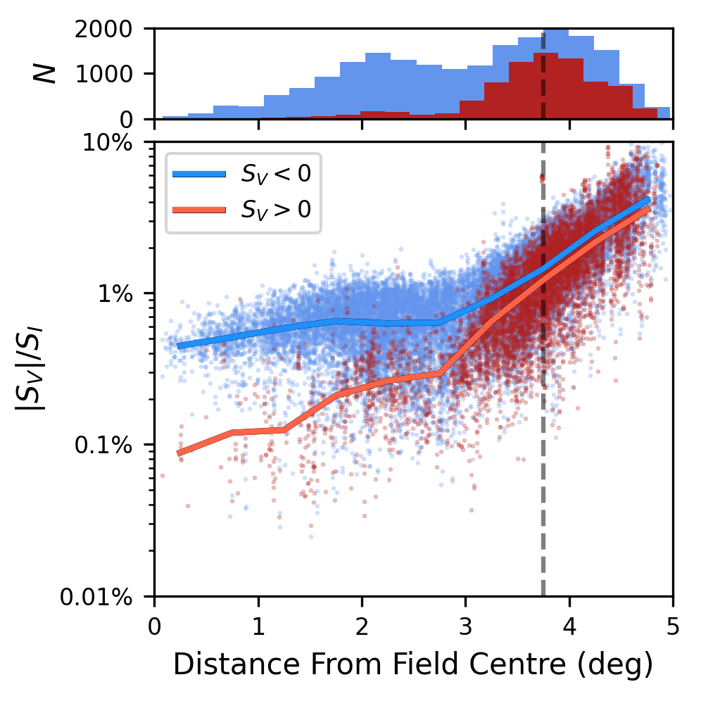
Figure 1: Leakage from Stokes $I$ into $V$ ($|S_{V}|/S_{I}$) as a function of angular distance from field centre. The points represent Stokes $I$-$V$ matches between isolated point sources with $S_{I}>$100\text{\,}\mathrm{mJy}\text{\,}{\mathrm{PSF}}^{-1}$$ with red and blue corresponding to matches with positive and negative Stokes $V$ flux respectively. The histograms show the distribution of positive and negative matches with angular distance with a bias towards negative leakage towards the field centre. The black dashed line indicates a field centre distance of $3.75\text{\,}\mathrm{\SIUnitSymbolDegree}$, within which the positive and negative leakage has median values of $0.6\text{\,}\mathrm{per~{}cent}$ and $-0.7\text{\,}\mathrm{per~{}cent}$ respectively.

We transformed the position of each sample into the image-centred frame to visualise the leakage pattern across the ASKAP field of view. In Figure 2 we show these samples alongside a Gaussian Process regression fit to the data with the position of all star and pulsar detections overlaid. Within the central $3.75\text{\,}\mathrm{\SIUnitSymbolDegree}$ from field centre the leakage has median positive and negative values of $0.6\text{\,}\mathrm{per~{}cent}$ and $-0.7\text{\,}\mathrm{per~{}cent}$. In this region the leakage pattern towards the edge of individual beams overlaps and suppresses the mosaiced leakage, with a small bias towards negative Stokes $V$ caused by imperfect overlap due to uncertainty in the primary beam response pattern. The tile edges have no overlapping beams and a residual leakage pattern is visible alternating between positive and negative Stokes $V$. We note that more recent ASKAP observations such as the mid-band epoch of RACS at $1367.5\text{\,}\mathrm{MHz}$ (RACS-mid; Duchesne et al., 2023) implement widefield leakage corrections that remove both the bias and residual leakage pattern.

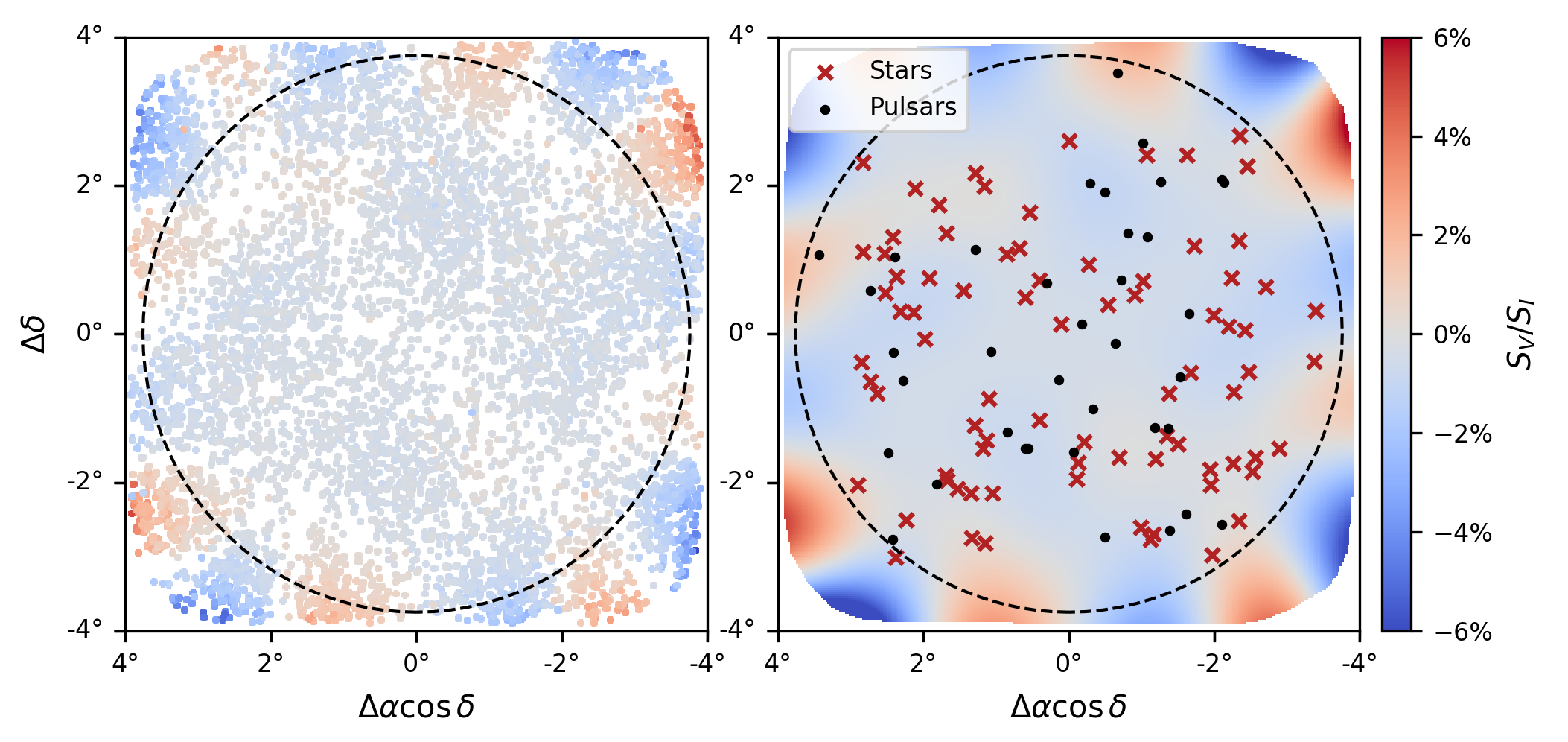
Figure 2: Map of leakage from Stokes $I$ into Stokes $V$ across the ASKAP field of view in VASTP-low. The left panel shows position and leakage of Stokes $I$-$V$ matches in the field-centred frame. The right panel shows a Gaussian Process regression model fit to these measurements, with the positions of all star and pulsar detections overlaid. The black dashed circle indicates an angular distance from the field centre of $3.75\text{\,}\mathrm{\SIUnitSymbolDegree}$.

3 CANDIDATE SEARCH

3.1 Candidate Selection

We generated associations between the extracted Stokes $I$ and $V$ components with a many-to-many crossmatch using a match radius of $6\text{\,}\arcsec$. Many-to-many association allows for one Stokes $I$ component to match to multiple Stokes $V$ components within the match radius (and vice versa), ensuring that all possible $I$-$V$ associations within the match radius are considered at the cost of an increased number of false-positive associations. This choice is made to avoid missing edge cases in which a near neighbour in Stokes $I$ matches on to the Stokes $V$ component and produces a lower $|S_{V}|/S_{I}$ than the correct Stokes $I$ component.

We then crossmatched the $I$-$V$ associations between each epoch to track individual candidates over the duration of the survey. Beginning with an initial epoch $A$ each $I$-$V$ association is assigned a unique association ID. We then generate an initial many-to-many crossmatch of $I$-$V$ associations between epoch $A$ and the subsequent epoch $B$ using the Stokes $I$ coordinates with a $6\text{\,}\arcsec$ match radius.

Many-to-many association across $N_{e}$ epochs results in $\mathcal{O}\left((n_{I}n_{V})^{N_{e}-1}\right)$ total candidates, with $n_{I}$ and $n_{V}$ selavy components within the match radius in Stokes $I$ and $V$ respectively. We de-duplicate these candidates by retaining only the $A$-$B$ associations whose match distance is the minimum of all duplicate candidates such that there is no other copy of an epoch $A$ or $B$ $I$-$V$ association with a closer match, reducing the number of candidates to $\mathcal{O}\left(\max(n_{I},n_{V})\right)$. This step greatly reduces the number of artefacts produced around bright sources, where $I$-$V$ associations between sidelobes shift position between epochs.

We create a running list of candidates for the epoch $A$-$B$ associations including epoch $A$ $I$-$V$ associations with no match in epoch $B$, and also add all epoch $B$ $I$-$V$ associations with no match in epoch $A$, assigning a new association ID. Finally we re-calculate the average Stokes $I$ coordinates of each candidate and use these to perform the next round of epoch-association. Using this procedure we performed association between the 15 epochs of VASTP-low, resulting in a list of $9\,818$ candidates. We then filtered this list to candidates both greater than $5\sigma$ in both Stokes $I$ and $V$ where $\sigma$ is the local RMS noise, and with at least one $I$-$V$ association with fractional circular polarisation $|S_{V}|/S_{I}>$6\text{\,}\mathrm{p}\mathrm{e}\mathrm{r}\mathrm{c}\mathrm{e}\mathrm{n}\mathrm{t}$$, corresponding to $10$ times the median polarisation leakage of Stokes $I$ into $V$ and three times the typical leakage of $\sim$$2\text{\,}\mathrm{per~{}cent}$ in image corners. Our final list contains 1 188 candidates.

3.2 Artefact Rejection

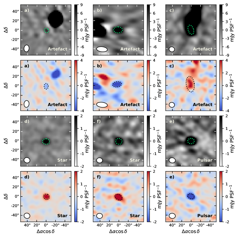
Figure 4: Stokes $I$ (top panel) and $V$ (bottom panel) cutouts of six candidates inspected during classification. The top pair of rows shows candidates rejected due to $I$-$V$ association between either the sidelobes of a bright source (panels a) and b)) or leakage from a multi-component extended source (panel c)). The bottom pair of rows show two identified stars (panels d) and e)) and a pulsar (panel f)) for comparison. The restoring beam is shown as the ellipse in the lower left of each panel, and green and black dotted ellipses trace the shape of the Stokes $I$ and $V$ selavy components in each association respectively.

Through visual inspection of the Stokes $I$ and $V$ images we rejected $I$-$V$ associations with artificially high $|S_{V}|/S_{I}$ caused by imaging artefacts and spurious noise. In Figure 4 we show a selection of example image cutouts of rejected artefacts as well as legitimately polarised sources. These artefacts are typically caused by one of the following situations:

• a match between a low flux component of a multi-component source in Stokes $I$ to leakage of a brighter component in Stokes $V$,

• a match between components of an extended source in Stokes $I$ and leakage in Stokes $V$, indicated by the presence of multiple nearby components and mismatched component shape parameters,

• a match to a spurious noise peak in Stokes $V$, indicated by a combination of low signal to noise ratio of $<6\sigma_{V}$ along with an offset between Stokes $I$ and $V$ position of $>4\arcsec$ and source morphology resembling noise rather than a point source,

• a match between the sidelobes and leakage of a poorly deconvolved bright source.

In total we removed 837 candidates based on these criteria, with the majority caused by matches between the sidelobes of bright sources in Stokes $I$ and their leakage in Stokes $V$ as shown in panels (a) and (b) of Figure 4, or association between leakage from the sub-components of an extended, multi-component source as shown in panel (c). We further removed 296 candidates with $|S_{V}|/S_{I}>0.06$ caused by polarisation leakage towards the image corners, where leakage is less well suppressed than the central region of the image.

3.3 Classification

We classified each of the remaining 54 candidates following the same procedure detailed by Pritchard et al. (2021); using radio and multi-wavelength image cutouts, queries to the SIMBAD and NED databases, and radio lightcurves and spectral energy distributions derived from archival radio data. We identified 85 total detections of 11 known pulsars, including the Large Magellanic Cloud pulsar PSR J0523$-$7125 discovered by Wang et al. (2022), and seven highly circularly polarised transients with no multi-wavelength counterpart, including the Galactic Centre transient J1736$-$3216 discovered by Wang et al. (2021).

We queried SIMBAD and the Gaia Data Release 3 (Gaia DR3; Gaia Collaboration et al., 2022) catalogue for stars within a $3\aas@@fstack{\prime}5$ radius of candidate positions. From this sample we removed sources with parallax over error $\pi/\sigma_{\pi}<10$ and distance $d<$500\text{\,}\mathrm{pc}$$ in order to reject false positive alignments to distant stars in high source density regions such as the Galactic plane. We then applied positional corrections to the radio epoch using Gaia proper motion parameters, identifying 36 matches to stars within the SNR dependent astrometric uncertainty determined by Equation 1.

Combined with the stars detected in our circular polarisation search of RACS-low we have detected a total of 76 radio stars. We quantified the rate of false-positive association between foreground stars and extra-galactic radio sources by offsetting the positions of all 76 stars by $520\text{\,}\mathrm{\SIUnitSymbolArcminute}$ in random directions and crossmatching against SIMBAD and Gaia DR3 with the same selection criteria as above. Ten runs of this procedure resulted in zero matches, suggesting a false-positive rate of less than $0.2\text{\,}\mathrm{per~{}cent}$ and an extremely low probability that any of our detections are due to chance alignment.

Table 3: Count summary of radio stars in RACS-low and VASTP-low. Columns indicate the abbreviated class name, number count of unique stars, total individual detections $N_{d}[I]$ and $N_{d}[V]$ in Stokes $I$ and $V$ respectively, and total observations $N_{o}$ for each variable class of radio star.

Variable Class		Stars	$N_{d}[I]$	$N_{d}[V]$	$N_{o}$
M-dwarfs	(dM)	45	96	65	417
RS CVn / Algol binaries	(IB)	9	52	23	74
Magnetic chemically peculiar	(MCP)	7	17	7	17
Young stellar objects	(YSO)	5	34	7	48
Hot spectroscopic binaries	(HSB)	4	23	4	32
K-dwarfs	(dK)	4	5	5	16
White dwarfs	(WD)	2	2	2	14

4 RADIO PROPERTIES

In our combined circular polarisation searches of RACS-low and VASTP-low we have detected 76 radio stars a total of 229 times in Stokes $I$ and 113 times in Stokes $V$. The majority of detected stars are M-dwarfs (dM) or interacting RS CVn / Algol binary systems (IB), with a small number of K-dwarfs (dK), YSOs, and MCP stars, and two white dwarfs (WD). We summarise the detection counts of each variable class detected in RACS-low and VASTP-low in Table 3, and in Table 4 we list the radio properties of each star.

We detect a higher proportion of dM to IB systems in comparison to radio stars detected in FIRST by Helfand et al. (1999) and LoTSS by Callingham et al. (2023), whose samples are each approximately $50\text{\,}\mathrm{per~{}cent}$ comprised of IB stars. This can be explained by the differences in survey strategy along with the relative timescales of dM and IB radio emission, where dM stars generally feature faint quiescent emission and radio bursts lasting seconds to hours (e.g. Villadsen & Hallinan, 2019), while IB systems typically have brighter, long-duration quiescent emission (e.g. Chiuderi Drago & Klein, 1990). FIRST observations are composed of $165\text{\,}\mathrm{s}$ snapshots co-added to an effective duration of $\sim$$35\text{\,}\mathrm{min}$ while the VASTP-low survey footprint is sampled a median of 14 times in $12\text{\,}\mathrm{min}$ snapshots, increasing the likelihood of detecting M-dwarf bursts. Moreover, FIRST observations covered a narrow bandwidth of $42\text{\,}\mathrm{MHz}$ which may have limited the capability to detect coherent M-dwarf bursts with sharp spectral cutoffs, while the detectability of broadband gyrosynchrotron emission associated with IB systems is less affected by bandwidth. LoTSS images are constructed with an integration time of $8\text{\,}\mathrm{h}$, and the M-dwarfs reported by Callingham et al. (2023) all feature long-duration emission spanning the full observation (Callingham et al., 2021b). Short time-scale bursts are likely to be missed in long integration images due to dilution of the burst flux with lengthy periods in which burst activity is low or absent. Alternatively, the difference in dM and IB detection counts may be explained by a change in the emission characteristics of each source class between the LoTSS frequency of $144\text{\,}\mathrm{MHz}$ and VASTP-low frequency of $887.5\text{\,}\mathrm{MHz}$, though further analysis of the radio stars detected in each band is required to disentangle survey strategy biases from intrinsic changes in the emission physics.

Table 4: Table of radio stars detected in the VASTP-low and RACS-low surveys. Listed columns are stellar name, radio variable and spectral classes, radio coordinates, proper motion parameters $\mu_{\alpha}\cos\delta$ and $\mu_{\delta}$, parallax $\pi$, upper limit to emission region length scale $R_{e}$, $887.5\text{\,}\mathrm{MHz}$ Stokes $I$ peak flux density $S_{I}$, fractional circular polarisation $|S_{V}|/S_{I}$, lower limit to brightness temperature $\log_{10}T_{B}$, radio luminosity $\log_{10}L_{\nu}$, and the number of Stokes $I$ and $V$ detections $N_{d}[I]$ and $N_{d}[V]$, and total number of observations $N_{o}$ of each star over the survey. $S_{I}$, $|S_{V}|/S_{I}$, $T_{B}$, and $L_{\nu}$ are reported as ranges over the detections of each star. A machine-readable version of this table is available online.

Name	Variable Type	Spectral Class	RA	Dec	$\mu_{\alpha}\cos\delta$	$\mu_{\delta}$	$\pi$	$R_{e}$a	$S_{I}$	$|S_{V}|/S_{I}$	$\log_{10}T_{B}$	$\log_{10}L_{\nu}$	$N_{d}[I]$	$N_{d}[V]$	$N_{o}$
					$\mathrm{m}\mathrm{a}\mathrm{s}\mathrm{/}\mathrm{yr}$	$\mathrm{m}\mathrm{a}\mathrm{s}\mathrm{/}\mathrm{yr}$	$\mathrm{m}\mathrm{a}\mathrm{s}$	$R_{\odot}$	$\mathrm{mJy}\text{\,}{\mathrm{PSF}}^{-1}$		$\mathrm{K}$	$\mathrm{erg}\text{\,}{\mathrm{s}}^{-1}\text{\,}{\mathrm{Hz}}^{-1}$
G 131-26	dM	M5V	00:08:53.88	$+$20:50:19.36	$~{}-48.64$	$-260.19$	$~{}~{}~{}55.26\pm 0.76$	$~{}~{}~{}1.0$	$2.78$	$0.57$	$10.3$	$15.0$	1	1	1
1RXS J001650.6-071013	dM	M0	00:16:50.11	$-$07:10:15.19	$~{}~{}~{}~{}39.84$	$~{}~{}~{}~{}~{}9.74$	$~{}~{}~{}14.01\pm 0.06$	$~{}~{}~{}2.3$	$0.85$–$3.07$	$0.19$–$1.00$	$10.3$–$10.9$	$15.7$–$16.3$	8	4	11
CF Tuc	IB	G2/5V+F0	00:53:09.12	$-$74:39:05.75	$~{}~{}~{}243.13$	$~{}~{}~{}~{}21.62$	$~{}~{}~{}11.37\pm 0.03$	$~{}~{}11.3$	$1.31$–$10.98$	$0.06$–$0.62$	$9.3$–$10.2$	$16.1$–$17.0$	10	1	10
CS Cet	dK	K0IV(e)	01:06:48.93	$-$22:51:23.22	$~{}-38.15$	$~{}-81.19$	$~{}~{}~{}10.50\pm 0.06$	$~{}~{}12.3$	$6.32$–$7.30$	$0.37$–$0.39$	$10.0$–$10.1$	$16.8$–$16.9$	2	2	2
BI Cet	IB	G5V	01:22:50.09	$+$00:42:39.60	$-114.59$	$-238.95$	$~{}~{}~{}15.98\pm 0.05$	$~{}~{}~{}4.8$	$1.20$–$3.45$	$0.21$–$0.99$	$9.7$–$10.2$	$15.8$–$16.2$	7	2	9
RX J0143.7-0602	dM	M3.5	01:43:45.14	$-$06:02:40.27	$~{}~{}~{}~{}52.26$	$~{}-27.07$	$~{}~{}~{}46.85\pm 0.07$	$~{}~{}~{}1.2$	$2.89$	$0.56$	$10.4$	$15.2$	1	1	13
WISEA J014358.01-014930.3	dM		01:43:58.02	$-$01:49:28.73	$~{}~{}~{}~{}60.35$	$~{}~{}~{}~{}~{}3.77$	$~{}~{}~{}24.80\pm 0.02$	$~{}~{}~{}1.0$	$1.44$	$0.84$	$10.7$	$15.4$	1	1	12
SDSS J020648.78-061416.3	IB		02:06:48.76	$-$06:14:16.30	$~{}~{}~{}~{}~{}6.13$	$~{}-24.34$	$~{}~{}~{}~{}2.25\pm 0.04$	$~{}~{}~{}4.8$	$1.64$	$0.96$	$11.6$	$17.6$	1	1	21
UPM J0250-0559	dM		02:50:40.29	$-$05:59:50.89	$~{}~{}~{}~{}67.31$	$~{}~{}~{}~{}10.17$	$~{}~{}~{}33.20\pm 0.96$	$~{}~{}~{}1.2$	$2.25$	$0.82$	$10.6$	$15.4$	1	1	24
LP  771-50	dM	M5e	02:56:27.19	$-$16:27:38.53	$~{}~{}~{}212.29$	$~{}-55.25$	$~{}~{}~{}32.56\pm 0.41$	$~{}~{}~{}0.6$	$1.65$	$1.00$	$11.1$	$15.3$	1	1	1
CD-44  1173	dM	K6Ve	03:31:55.73	$-$43:59:14.91	$~{}~{}~{}~{}88.47$	$~{}~{}-3.50$	$~{}~{}~{}22.17\pm 0.03$	$~{}~{}~{}2.5$	$3.87$	$0.88$	$10.5$	$16.0$	1	1	19
HD  22468	IB	K2:Vnk	03:36:47.19	$+$00:35:13.52	$~{}-32.89$	$-161.77$	$~{}~{}~{}33.75\pm 0.09$	$~{}~{}~{}9.1$	$6.92$–$78.17$	$0.03$–$0.54$	$9.3$–$10.3$	$15.9$–$16.9$	13	13	13
RX J0348.9+0110	dK	K3V:/E	03:48:58.83	$+$01:10:54.83	$~{}~{}~{}~{}29.73$	$~{}-22.72$	$~{}~{}~{}~{}9.11\pm 0.33$	$~{}~{}~{}0.9$	$1.42$	$0.93$	$11.8$	$16.3$	1	1	12
HD  24681	YSO	G5V	03:55:20.61	$-$01:43:46.58	$~{}~{}~{}~{}43.33$	$~{}-91.49$	$~{}~{}~{}17.82\pm 0.04$	$~{}~{}~{}2.6$	$1.88$	$0.54$	$10.3$	$15.9$	1	1	13
HD  24916B	dM	M2.5V	03:57:28.66	$-$01:09:27.07	$-209.41$	$-139.73$	$~{}~{}~{}65.49\pm 0.04$	$~{}~{}~{}1.3$	$1.02$	$0.91$	$9.5$	$14.5$	1	1	13
UPM J0409-4435	dM		04:09:32.15	$-$44:35:38.19	$~{}-16.86$	$~{}~{}~{}115.59$	$~{}~{}~{}68.07\pm 0.04$	$~{}~{}~{}0.7$	$1.27$–$2.42$	$0.73$–$1.00$	$10.2$–$10.4$	$14.5$–$14.8$	3	1	23
RX J0419.2-7120	dM		04:19:13.35	$-$71:21:12.05	$~{}-52.92$	$~{}-46.71$	$~{}~{}~{}18.77\pm 0.13$	$~{}~{}~{}1.1$	$1.45$	$0.58$	$10.9$	$15.7$	1	1	1
HD 283750	dK	K2.5Ve	04:36:48.60	$+$27:07:55.01	$~{}~{}~{}232.87$	$-148.14$	$~{}~{}~{}57.10\pm 0.06$	$~{}~{}~{}2.0$	$3.94$	$0.76$	$9.9$	$15.2$	1	1	1
CD-56  1032	dM	M3Ve+M4Ve	04:53:31.02	$-$55:51:35.10	$~{}~{}~{}126.12$	$~{}~{}~{}~{}76.86$	$~{}~{}~{}90.12\pm 0.03$	$~{}~{}~{}1.3$	$0.96$–$12.38$	$0.16$–$0.98$	$9.3$–$10.4$	$14.1$–$15.3$	14	2	23
HD  32595	HSB	B8	05:04:49.06	$+$13:18:32.86	$~{}~{}~{}~{}~{}1.83$	$~{}~{}-5.18$	$~{}~{}~{}~{}3.40\pm 0.28$	$~{}~{}~{}6.5$	$3.36$	$0.62$	$11.2$	$17.5$	1	1	1
V1154 Tau	IB	B5	05:05:37.70	$+$23:03:41.59	$~{}~{}~{}~{}~{}0.27$	$~{}~{}-6.89$	$~{}~{}~{}~{}3.59\pm 0.46$	$~{}~{}~{}8.9$	$2.07$	$0.64$	$10.7$	$17.3$	1	1	1
AB Dor	YSO	K0V	05:28:44.98	$-$65:26:51.35	$~{}~{}~{}~{}29.15$	$~{}~{}~{}164.42$	$~{}~{}~{}65.32\pm 0.14$	$~{}~{}~{}4.5$	$1.83$–$7.73$	$0.16$–$1.00$	$8.7$–$9.4$	$14.7$–$15.3$	29	2	31
HD  36150	MCP	A5III/IV	05:29:41.78	$-$00:48:07.66	$~{}~{}~{}~{}71.34$	$~{}-47.04$	$~{}~{}~{}~{}8.93\pm 0.18$	$~{}~{}~{}8.9$	$1.99$	$1.00$	$9.9$	$16.5$	1	1	1
SCR J0533-4257	dM	M4.5	05:33:28.01	$-$42:57:18.93	$~{}-17.58$	$~{}~{}~{}~{}39.51$	$~{}~{}~{}96.63\pm 0.34$	$~{}~{}~{}1.4$	$0.85$–$6.32$	$0.57$–$1.00$	$9.1$–$10.0$	$14.0$–$14.9$	7	4	12
$[$W60$]$ D43	dM	M	05:35:36.96	$-$67:05:23.00					$1.41$	$0.74$			1	1	10
Ross  614	dM	M4.5V	06:29:24.31	$-$02:49:03.32	$~{}~{}~{}750.14$	$-802.95$	$~{}~{}242.97\pm 0.88$	$~{}~{}~{}0.8$	$2.75$–$3.84$	$0.39$–$0.55$	$9.3$–$9.5$	$13.7$–$13.9$	2	2	2
Gaia DR3 2930889294867085440	WD		07:15:31.16	$-$19:39:53.82	$~{}~{}-6.06$	$~{}~{}~{}~{}16.22$	$~{}~{}~{}~{}5.52\pm 0.21$	$~{}~{}~{}0.03$	$12.39$	$0.43$	$16.0$	$17.7$	1	1	1
alf Gem	HSB	A1V+A2Vm	07:34:35.49	$+$31:53:14.63			$~{}~{}~{}64.12\pm 3.75$	$~{}~{}~{}6.8$	$1.35$	$0.78$	$8.3$	$14.6$	1	1	1
k02 Pup	MCP	B5IV	07:38:49.74	$-$26:48:12.84	$~{}-17.54$	$~{}~{}~{}~{}21.36$	$~{}~{}~{}~{}8.81\pm 0.20$	$~{}~{}~{}5.3$	$2.93$	$0.76$	$10.5$	$16.7$	1	1	1
YZ CMi	dM	M4.0Ve	07:44:39.66	$+$03:33:01.74	$-348.10$	$-445.88$	$~{}~{}167.02\pm 0.06$	$~{}~{}~{}1.1$	$2.66$	$1.00$	$9.3$	$14.1$	1	1	1
HD  67951	MCP	ApSiCr	08:08:23.62	$-$45:47:43.16	$~{}~{}-4.29$	$~{}~{}~{}~{}~{}9.96$	$~{}~{}~{}~{}2.65\pm 0.04$	$~{}~{}~{}1.8$	$3.13$	$0.40$	$12.6$	$17.7$	1	1	1
G  41-14	dM	M3.5V	08:58:56.75	$+$08:28:19.76			$~{}~{}147.66\pm 1.98$	$~{}~{}~{}0.8$	$19.19$	$0.89$	$10.6$	$15.0$	1	1	1
HD  77653	MCP	ApSi	09:01:44.44	$-$52:11:19.82			$~{}~{}~{}~{}8.85\pm 0.42$	$~{}~{}~{}4.7$	$7.06$	$0.67$	$11.0$	$17.0$	1	1	1
WT 2458	dM	M4.5	09:45:57.98	$-$32:53:26.40	$-300.41$	$~{}~{}~{}146.02$	$~{}~{}~{}83.23\pm 0.09$	$~{}~{}~{}0.7$	$1.54$	$0.83$	$10.1$	$14.4$	1	1	1
PM J09551-0819	dM	M1e	09:55:09.49	$-$08:19:23.93	$-135.78$	$~{}~{}-7.16$	$~{}~{}~{}31.49\pm 0.04$	$~{}~{}~{}0.8$	$1.81$	$0.84$	$10.9$	$15.3$	1	1	25
LP  610-59	dM		10:43:37.55	$-$00:48:09.06	$-184.94$	$~{}~{}~{}~{}14.43$	$~{}~{}~{}19.53\pm 0.15$	$~{}~{}~{}0.6$	$2.05$	$0.76$	$11.6$	$15.8$	1	1	24
WISEA J105315.25-085941.5	dM		10:53:15.20	$-$08:59:42.22	$~{}~{}~{}~{}30.96$	$~{}~{}-0.67$	$~{}~{}~{}29.38\pm 0.06$	$~{}~{}~{}1.0$	$1.07$–$3.43$	$0.59$–$0.95$	$10.5$–$11.0$	$15.2$–$15.7$	3	1	11
ksi UMa	IB	F8.5:V+G2V	11:18:10.18	$+$31:31:31.12	$-339.40$	$-607.89$	$~{}~{}114.49\pm 0.43$	$~{}~{}11.3$	$1.49$	$0.68$	$7.4$	$14.1$	1	1	1
WISEA J114020.71-330519.4	dM		11:40:20.68	$-$33:05:19.22	$~{}-62.94$	$~{}-29.30$	$~{}~{}~{}12.94\pm 0.08$	$~{}~{}~{}0.9$	$2.54$	$0.63$	$11.7$	$16.3$	1	1	1

Table 5: Table 4 continued.

Name	Variable Type	Spectral Class	RA	Dec	$\mu_{\alpha}\cos\delta$	$\mu_{\delta}$	$\pi$	$R_{e}$a	$S_{I}$	$|S_{V}|/S_{I}$	$\log_{10}T_{B}$	$\log_{10}L_{\nu}$	$N_{d}[I]$	$N_{d}[V]$	$N_{o}$
					$\mathrm{m}\mathrm{a}\mathrm{s}\mathrm{/}\mathrm{yr}$	$\mathrm{m}\mathrm{a}\mathrm{s}\mathrm{/}\mathrm{yr}$	$\mathrm{m}\mathrm{a}\mathrm{s}$	$R_{\odot}$	$\mathrm{mJy}\text{\,}{\mathrm{PSF}}^{-1}$		$\mathrm{K}$	$\mathrm{erg}\text{\,}{\mathrm{s}}^{-1}\text{\,}{\mathrm{Hz}}^{-1}$
PM J11422-0122	dM	M5e	11:42:12.84	$-$01:22:05.61	$~{}-98.06$	$~{}~{}-4.86$	$~{}~{}~{}54.07\pm 0.66$	$~{}~{}~{}0.3$	$2.31$	$0.41$	$11.3$	$15.0$	1	1	14
HD 105382	MCP	B5V	12:08:05.06	$-$50:39:40.79	$~{}-34.35$	$~{}-11.51$	$~{}~{}~{}~{}9.85\pm 0.32$	$~{}~{}~{}5.0$	$2.28$	$0.59$	$10.4$	$16.4$	1	1	1
WISEA J122501.45-521614.6	dM		12:25:01.37	$-$52:16:14.58	$~{}-30.86$	$~{}-11.29$	$~{}~{}~{}~{}8.14\pm 0.30$	$~{}~{}~{}0.4$	$3.40$	$0.86$	$13.0$	$16.8$	1	1	1
WISEA J123623.17-074508.2	dM		12:36:23.03	$-$07:45:06.81	$~{}-83.14$	$~{}-34.91$	$~{}~{}~{}25.17\pm 0.06$	$~{}~{}~{}0.7$	$2.28$	$0.60$	$11.2$	$15.6$	1	1	10
UCAC4 129-071513	YSO		12:52:22.67	$-$64:18:38.92	$~{}-38.42$	$~{}-14.69$	$~{}~{}~{}~{}9.70\pm 0.06$	$~{}~{}~{}2.0$	$1.38$–$3.36$	$0.84$–$1.00$	$11.0$–$11.4$	$16.2$–$16.6$	2	2	2
HD 115247	HSB	F5V	13:16:02.96	$-$05:40:07.91	$~{}-83.66$	$~{}-40.39$	$~{}~{}~{}~{}8.41\pm 0.06$	$~{}~{}10.4$	$2.23$–$9.87$	$0.06$–$0.53$	$9.9$–$10.5$	$16.6$–$17.2$	20	1	21
BH CVn	IB	A6m	13:34:47.90	$+$37:10:56.77	$~{}~{}~{}~{}85.61$	$~{}~{}-9.71$	$~{}~{}~{}21.67\pm 0.16$	$~{}~{}~{}9.8$	$6.64$–$7.16$	$0.35$–$0.37$	$9.6$–$9.6$	$16.2$–$16.3$	2	2	2
V851 Cen	IB	K0III	13:44:00.95	$-$61:21:58.92	$~{}~{}~{}~{}21.07$	$~{}~{}~{}~{}13.80$	$~{}~{}~{}13.50\pm 0.04$	$~{}~{}10.6$	$7.68$	$0.69$	$10.0$	$16.7$	1	1	1
CU Vir	MCP	ApSi	14:12:15.72	$+$02:24:34.21	$~{}-43.05$	$~{}-26.08$	$~{}~{}~{}13.94\pm 0.26$	$~{}~{}~{}6.3$	$2.17$–$13.83$	$0.16$–$0.64$	$9.9$–$10.7$	$16.1$–$16.9$	11	1	11
HD 124498	dK	K5.5Vkee	14:14:21.74	$-$15:21:17.96	$-128.33$	$-164.99$	$~{}~{}~{}34.53\pm 0.18$	$~{}~{}~{}2.3$	$2.17$	$0.62$	$10.0$	$15.3$	1	1	1
WISEA J141443.13+261639.7	dM		14:14:43.16	$+$26:16:40.45	$~{}~{}~{}~{}55.60$	$~{}~{}-3.50$	$~{}~{}~{}21.26\pm 0.06$	$~{}~{}~{}0.8$	$2.65$–$3.08$	$0.62$–$0.72$	$11.3$–$11.4$	$15.8$–$15.9$	2	2	2
G 165-61	dM	M4.5Ve	14:17:02.04	$+$31:42:44.31			$~{}~{}~{}60.00\pm 2.20$	$~{}~{}~{}0.6$	$2.02$	$0.96$	$10.6$	$14.8$	1	1	1
G 124-43	dM	M4.65	14:27:55.67	$-$00:22:26.29	$-361.50$	$~{}~{}~{}~{}41.64$	$~{}~{}~{}57.08\pm 0.06$	$~{}~{}~{}1.0$	$1.30$–$2.97$	$0.40$–$1.00$	$10.0$–$10.4$	$14.7$–$15.0$	9	5	22
LP  325-68	dM	M4.5Ve	14:37:18.08	$+$26:53:00.87	$-227.64$	$~{}~{}~{}~{}84.35$	$~{}~{}~{}27.29\pm 0.06$	$~{}~{}~{}0.8$	$3.01$	$0.55$	$11.2$	$15.7$	1	1	1
HD 142184	MCP	B2V	15:53:55.82	$-$23:58:41.33	$~{}-13.47$	$~{}-23.97$	$~{}~{}~{}~{}7.08\pm 0.14$	$~{}~{}11.7$	$7.84$	$0.22$	$10.5$	$17.3$	1	1	1
GSS 35	YSO	B3	16:26:34.11	$-$24:23:28.17	$~{}~{}-2.17$	$~{}-23.56$	$~{}~{}~{}~{}8.17\pm 0.11$	$~{}~{}~{}2.5$	$8.18$	$0.23$	$11.7$	$17.2$	1	1	1
EMSR   20	YSO	G7	16:28:32.50	$-$24:22:45.81	$~{}~{}-9.47$	$~{}-28.06$	$~{}~{}~{}~{}7.35\pm 0.06$	$~{}~{}~{}2.4$	$2.24$	$0.72$	$11.3$	$16.7$	1	1	1
CD-38 11343	dM	M3Ve+M4Ve	16:56:48.49	$-$39:05:38.96	$~{}~{}~{}~{}47.00$	$-113.26$	$~{}~{}~{}63.63\pm 0.08$	$~{}~{}~{}1.3$	$7.29$	$0.29$	$10.4$	$15.3$	1	1	1
PM J17021-2740	dM		17:02:07.97	$-$27:40:28.71	$-129.85$	$-220.40$	$~{}~{}~{}41.86\pm 0.09$	$~{}~{}~{}0.9$	$3.99$	$0.68$	$10.9$	$15.4$	1	1	1
Ross  867	dM	M4.5V	17:19:52.68	$+$26:30:09.94	$-226.13$	$~{}~{}~{}355.28$	$~{}~{}~{}92.97\pm 0.06$	$~{}~{}~{}0.9$	$3.79$	$0.67$	$10.2$	$14.7$	1	1	1
G 183-10	dM	M3.5Ve	17:53:00.25	$+$16:54:59.05	$-243.94$	$-240.05$	$~{}~{}~{}44.15\pm 1.02$	$~{}~{}~{}0.8$	$2.09$	$0.51$	$10.6$	$15.1$	1	1	1
2MASS J18040683-1211342	dM		18:04:06.89	$-$12:11:35.71	$~{}-28.06$	$~{}~{}-6.91$	$~{}~{}~{}18.52\pm 0.04$	$~{}~{}~{}0.9$	$2.71$	$0.64$	$11.4$	$16.0$	1	1	1
UCAC3 152-281176	dM	M5	18:45:00.95	$-$14:09:04.59	$~{}~{}~{}~{}47.60$	$~{}-85.72$	$~{}~{}~{}54.97\pm 0.09$	$~{}~{}~{}0.9$	$5.73$	$0.79$	$10.8$	$15.4$	1	1	2
SCR J1928-3634	dM		19:28:33.74	$-$36:34:39.21	$~{}~{}~{}~{}95.72$	$-453.66$	$~{}~{}~{}39.55\pm 0.06$	$~{}~{}~{}0.7$	$2.51$	$0.64$	$10.9$	$15.3$	1	1	1
2MASS J19551247+0045365	WD		19:55:12.45	$+$00:45:36.33	$~{}~{}-2.55$	$~{}-29.55$	$~{}~{}~{}~{}5.85\pm 0.08$	$~{}~{}~{}0.07$	$2.19$	$0.69$	$14.6$	$16.9$	1	1	13
bet Aql B	dM	M3	19:55:18.83	$+$06:24:28.14	$~{}~{}~{}~{}22.62$	$-472.30$	$~{}~{}~{}73.61\pm 0.05$	$~{}~{}~{}1.2$	$2.85$	$0.74$	$9.9$	$14.8$	1	1	1
SCR J2009-0113	dM	M5.0V	20:09:18.16	$-$01:13:45.36	$~{}-43.63$	$-373.73$	$~{}~{}~{}92.52\pm 0.12$	$~{}~{}~{}0.6$	$1.86$–$10.30$	$0.73$–$0.92$	$10.3$–$11.0$	$14.4$–$15.2$	5	5	12
LEHPM 2-783	dM	M6	20:19:49.81	$-$58:16:49.89	$~{}-24.64$	$-340.82$	$~{}~{}~{}61.18\pm 0.10$	$~{}~{}~{}1.0$	$2.43$	$0.81$	$10.2$	$14.9$	1	1	12
2MASS J20390476-4117390	dM		20:39:04.97	$-$41:17:38.95	$~{}~{}~{}~{}58.05$	$~{}-47.38$	$~{}~{}~{}25.63\pm 0.06$	$~{}~{}~{}0.7$	$1.67$	$0.99$	$11.1$	$15.5$	1	1	12
Ross  776	dM	M3.3V	21:16:06.14	$+$29:51:52.37	$~{}~{}~{}204.61$	$~{}~{}~{}~{}24.16$	$~{}~{}~{}49.21\pm 0.24$	$~{}~{}~{}1.3$	$6.44$	$0.50$	$10.6$	$15.5$	1	1	1
UCAC3 89-412162	dM		21:22:17.56	$-$45:46:31.42	$~{}-53.47$	$~{}-34.00$	$~{}~{}~{}31.55\pm 0.04$	$~{}~{}~{}0.8$	$2.31$	$0.87$	$11.0$	$15.4$	1	1	12
HD 210547A	HSB		22:13:00.08	$-$61:58:53.05	$~{}-13.18$	$~{}~{}~{}~{}~{}0.79$	$~{}~{}~{}~{}5.82\pm 0.03$	$~{}~{}~{}5.7$	$1.44$	$0.94$	$10.5$	$16.7$	1	1	9
Wolf 1561 A	dM	M4V	22:17:18.29	$-$08:48:18.13	$-458.51$	$-291.85$	$~{}~{}~{}89.80\pm 0.09$	$~{}~{}~{}0.7$	$1.74$–$1.85$	$0.69$–$1.00$	$10.0$–$10.1$	$14.4$–$14.4$	2	1	14
LAMOST J221747.87-030039.0	dM	M5	22:17:47.86	$-$03:00:38.82	$~{}~{}~{}~{}21.79$	$~{}~{}-9.96$	$~{}~{}~{}~{}6.71\pm 0.08$	$~{}~{}~{}1.3$	$5.50$	$0.77$	$12.2$	$17.2$	1	1	36
UPM J2224-5826	dM		22:24:24.51	$-$58:26:14.13	$~{}-75.71$	$~{}-37.18$	$~{}~{}~{}62.38\pm 0.19$	$~{}~{}~{}1.5$	$4.12$–$5.45$	$0.85$–$1.00$	$10.1$–$10.2$	$15.1$–$15.2$	2	1	20
SCR J2241-6119A	dM		22:41:44.76	$-$61:19:33.18	$~{}~{}~{}150.23$	$~{}-87.90$	$~{}~{}~{}35.19\pm 0.05$	$~{}~{}~{}0.9$	$1.38$–$5.44$	$0.39$–$1.00$	$10.6$–$11.2$	$15.1$–$15.7$	6	4	9
SZ Psc	IB	G5Vp	23:13:23.70	$+$02:40:33.01	$~{}~{}~{}~{}27.03$	$~{}~{}~{}~{}27.33$	$~{}~{}~{}11.10\pm 0.08$	$~{}~{}13.7$	$2.07$–$11.89$	$0.03$–$0.84$	$9.4$–$10.1$	$16.3$–$17.1$	16	1	16

• $R_{e}$ taken as: $3R_{\star}$ for single stars as calculated from Gaia DR3 photometry (Gaia Collaboration et al., 2022) and the inter-binary region for interacting binaries.

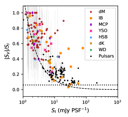
Figure 3: Fractional circular polarisation and flux density phase space, with the radio stars in our sample labelled according to variable class. M-dwarfs (dM) are shown as red stars, K-dwarfs (dK) as brown stars, interacting binaries (IB) as yellow squares, magnetic chemically peculiar (MCP) stars as purple diamonds, young stellar objects (YSO) as fuchsia crosses, hot spectroscopic binaries (HSB) as blue triangles, and white dwarfs (WD) as green hexagons. The dotted line indicates a fractional circular polarisation of $6\text{\,}\mathrm{per~{}cent}$ below which we excluded candidates from initial classification, retaining only the low $|S_{V}|/S_{I}$ detections of previously classified sources. The dashed line indicates a $5\sigma_{V}$ detection threshold where $\sigma_{V}=$0.25\text{\,}\mathrm{mJy}\text{\,}{\mathrm{PSF}}^{-1}$$ is the median RMS noise in Stokes $V$, and represents the average sensitivity limit in fractional polarisation across our survey. Local variations in RMS result in a few detections below this threshold.

In Figure 3 we show the fractional circular polarisation $|S_{V}|/S_{I}$ as a function of Stokes $I$ flux density for all star detections in RACS-low and VASTP-low. We also show detected pulsars that are well separated in this space from the majority of single star detections, having lower $|S_{V}|/S_{I}$ of ${\sim}$1030\text{\,}\mathrm{per~{}cent}$$. This is slightly higher than the fractional circular polarisation of pulsars detected in LoTSS by Callingham et al. (2023), who find most pulsars below the $|S_{V}|/S_{I}\sim$10\text{\,}\mathrm{per~{}cent}$$ level, however this is likely just a selection effect due to the $|S_{V}|/S_{I}\sim$6\text{\,}\mathrm{per~{}cent}$$ limit of our search. For a more complete analysis of known pulsars detected in RACS-low we refer the reader to Anumarlapudi et al. (2023), who find a mean pulsar $|S_{V}|/S_{I}$ of $\sim$5\text{\,}\mathrm{per~{}cent}$$.

In Figure 5 we show the Stokes $I$ radio luminosity distribution of our sample, with M-dwarfs tending to group around $L_{\nu}=${10}^{15}\text{\,}\mathrm{erg}\text{\,}{\mathrm{s}}^{-1}\text{\,}{\mathrm{Hz}}^{-1}$$ while other variable types group around $L_{\nu}=${10}^{16}{10}^{17}\text{\,}\mathrm{erg}\text{\,}{\mathrm{s}}^{-1}\text{\,}{\mathrm{Hz}}^{-1}$$. Radio luminosity is also shown as a function of stellar distance in Figure 6. The hatched region represents flux densities below our $5\sigma$ detection threshold of $1.25\text{\,}\mathrm{mJy}\text{\,}{\mathrm{PSF}}^{-1}$ in Stokes $I$, which preferentially suppresses counts at the low end of the $L_{\nu}$ distribution. The completeness of our sample is further dependent upon fractional circular polarisation, with lower $|S_{V}|/S_{I}$ shifting the detection threshold to higher $L_{\nu}$, indicated by the dashed line at $|S_{V}|/S_{I}=0.5$.

To place constraints on plausible radio emission mechanisms we calculated the brightness temperature

$$T_{B}=\frac{Sc^{2}}{2\pi k_{B}\nu^{2}}\frac{d^{2}}{R_{e}^{2}}$$ (2)

where $k_{B}$ is the Boltzmann constant, $\nu$ is the observing frequency of $887.5\text{\,}\mathrm{MHz}$, $d$ is the stellar distance, and $R_{e}$ is the length scale of the emission region. We have assumed an upper limit of $R_{e}=3R_{\star}$ for each star, and additionally calculate $T_{B}$ for interacting binaries with $R_{e}$ equal to three times the binary separation distance. The true emission region is likely much smaller than these limits, particularly for detections with large $|S_{V}|/S_{I}$ as they require a consistent orientation of the magnetic field within the emission region to produce predominantly right or left handed circular polarisation.

In Figure 7 we show all star detections in a brightness temperature–fractional circular polarisation phase space alongside empirical models of the maximum effective temperature of optically thin gyrosynchrotron emission (Dulk, 1985). Most interacting binary systems feature minimum $T_{B}$ of ${10}^{6}{10}^{10}\text{\,}\mathrm{K}$ and $|S_{V}|/S_{I}<0.8$ and are plausibly driven by gyrosynchrotron emission which is commonly detected from RS CVn systems, though we note that coherent emission from the ECMI is also possible (e.g. Slee et al., 2008; Toet et al., 2021). The majority of other detections including one RS CVn, however, feature minimum $T_{B}$ of order ${10}^{10}{10}^{16}\text{\,}\mathrm{K}$, and as these detections feature high fractional circular polarisation the emission necessarily originates from a compact region in which the magnetic field is nearly uniform. This constraint on the size of the emission region further increases the minimum brightness temperature, and combined with the large fractional circular polarisation makes gyrosynchrotron emission unlikely. These detections are therefore likely driven by a coherent emission process such as the ECMI or plasma emission.

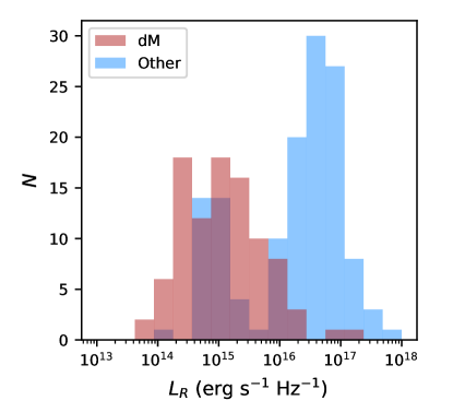
Figure 5: Stokes $I$ radio luminosity distribution of all star detections in RACS-low and VASTP-low. M-dwarfs are shown in red and all other stars are combined and shown in blue, as the sample sizes of individual variable and spectral classes are too low to meaningfully show them separately.

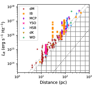
Figure 6: Stokes $I$ radio luminosity of each star detection as a function of distance. The hatched region corresponds to Stokes $I$ flux densities below the $5\sigma$ detection threshold of $1.25\text{\,}\mathrm{mJy}\text{\,}{\mathrm{PSF}}^{-1}$. The dashed line indicates the $5\sigma$ Stokes $V$ detection threshold for $|S_{V}|/S_{I}=0.5$, with lower $|S_{V}|/S_{I}$ shifting the threshold to higher $L_{\nu}$. The dotted line represents the projected $5\sigma$ detection threshold of $22\text{\,}\mathrm{\SIUnitSymbolMicro Jy}\text{\,}{\mathrm{PSF}}^{-1}$ in a $1\text{\,}\mathrm{h}$ observation with SKA-mid (Braun et al., 2019). Repeat detections are visible as vertically aligned points.

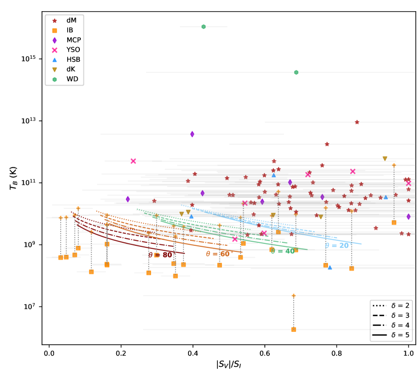
Figure 7: Brightness temperature and fractional circular polarisation phase space, with stars labelled according to variable class (see Figure 3). Vertical dotted lines connect two $T_{B}$ estimates for interacting binary systems, with estimated emission regions of the inter-binary region and stellar disk represented as yellow squares and crosses respectively. Empirical models of the maximum effective temperature of optically thin gyro-synchrotron emission (Dulk, 1985) are shown for a range of electron energy index $\delta$ and viewing angle $\theta$.

5 POPULATION STATISTICS

5.1 Detection Counts

We detected a total of 36 stars within the VASTP-low footprint over 15 epochs. Due to slight variations in the survey footprint between epochs and overlap between neighbouring tiles, each star was observed between 9–36 times with a median of 14 observations. To characterise the repeat detection rates of each star we calculate the detection fraction $DF=N_{d}/N_{o}$ where $N_{o}$ and $N_{d}$ are the respective number of observations and detections of each star. These counts only consider observations in which the local 3-sigma RMS noise is less than the flux density of the weakest detection, removing observations in which the star is located toward the image edges or corners where sensitivity degrades.

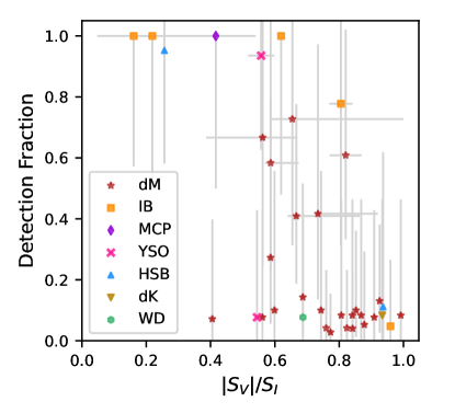
Figure 8: Detection fraction as a function of fractional circular polarisation for our sample of repeat observed stars in the VASTP-low footprint. The $|S_{V}|/S_{I}$ error bars indicate the range of observed fractional circular polarisation for each star, and the detection fraction error bars are derived from $95\text{\,}\mathrm{per~{}cent}$ Poisson confidence intervals on the number of detections. Markers denote the sub-type of variable star (see Figure 3).

In Figure 8 we show the detection fraction as a function of fractional polarisation. Most of the stars with high $DF$ are interacting binaries that feature a quiescent component to the radio emission, along with one YSO (AB Dor) and one MCP star (CU Vir) that are both well-known, persistent radio emitters. We find the majority of highly circularly polarised detections are associated with single detections of M-dwarfs with a median $DF$ of $8.5\text{\,}\mathrm{per~{}cent}$, and take this as an upper limit on the average population detection fraction $\langle DF\rangle$. This upper limit is consistent with previous estimates of the duty cycle of both stochastic radio bursts (Villadsen & Hallinan, 2019) and rotationally modulated auroral emission (Hallinan et al., 2007; Nichols et al., 2012).

5.2 Radio Activity Fraction of the M-Dwarf Population

As we detect new stars in each successive analysed epoch, an upper limit to the detection fraction implies the existence of low burst-rate stars within the population that produce detectable radio bursts but have not been sufficiently sampled to produce a detection. We define a burst to be detectable if it has a radio luminosity sufficient to be detected above our $5\sigma$ detection threshold of $1.25\text{\,}\mathrm{mJy}\text{\,}{\mathrm{PSF}}^{-1}$, which corresponds to a detectability horizon $d_{\rm max}$ for a particular burst radio luminosity. In this section we use the repeat detection rates of stars within the VASTP-low footprint to estimate the size of the detectable population. We limit our analysis to M-dwarfs due to the low sample size of other variable and spectral classes. We further restrict our sample to $d_{\rm max}<$25\text{\,}\mathrm{pc}$$ within which bursts above the typical M-dwarf radio luminosity of ${10}^{15}\text{\,}\mathrm{erg}\text{\,}{\mathrm{s}}^{-1}\text{\,}{\mathrm{Hz}}^{-1}$ are detectable, as our sample becomes increasingly incomplete in radio luminosity at greater distances.

We assume there are $n$ detectable M-dwarfs per unit solid angle, each with a burst rate $\lambda$ sampled from the population distribution $f(\lambda)$ such that $nAf(\lambda)\,\mathrm{d}{\lambda}$ is the number of detectable M-dwarfs with burst rates between $\lambda$ and $\lambda+\,\mathrm{d}{\lambda}$ in a solid angle $A$. For a star with rate $\lambda$ the number of detectable bursts in an epoch of duration $\Delta t$ is $\lambda\Delta t$. Hence the expected number of bursts detected in the epoch from all stars in a solid angle $A$ is

$$N_{d} =\int_{0}^{\infty}nA\lambda\Delta tf(\lambda)\,\mathrm{d}{\lambda}$$ (3)

$$=nA\Delta t\langle\lambda\rangle$$ (4)

where $\langle\lambda\rangle=\int_{0}^{\infty}\lambda f(\lambda)\,\mathrm{d}{\lambda}$ is the average burst rate over the observed stars. The expected number of bursts in $M$ epochs is then

$$\sum_{i=1}^{M}N_{d,i} =n\langle\lambda\rangle\sum_{i=1}^{M}A_{i}\Delta t_{i}$$ (5)

where $A_{i}$ and $\Delta t_{i}$ are the solid angle coverage and observation duration of epoch $i$.

None of our detections show evidence of bursts on timescales shorter than the observation time so we assume each detection represents a single burst, and as our RACS-low detections are all bright enough to be detected in a $12\text{\,}\mathrm{min}$ observation we adopt a common $\Delta t=$12\text{\,}\mathrm{min}$$ for all epochs. The average detection fraction $\langle DF\rangle$ is then an estimate of the average burst rate:

$$\langle\lambda\rangle=\frac{\langle DF\rangle}{\Delta t},$$ (6)

and the total number of detectable M-dwarfs in the VASTP-low footprint of area $A_{S}=$5131\text{\,}\deg^{2}$$ is then, using Equations 5 and 6:

$$\mathcal{N}=nA_{S} =\frac{A_{S}}{{\sum_{i=1}^{M}A_{i}}}\frac{1}{\langle DF\rangle}\sum_{i=1}^{M}N_{d,i}.$$ (7)

Within $25\text{\,}\mathrm{pc}$ we detect 11 M-dwarfs a total of 46 times. Using the solid angle coverage of each epoch listed in Table 2 with Equation 7 we estimate at least $\mathcal{N}=$ ${47}^{\thinspace+{16}}_{-{13}}$ M-dwarfs within the VASTP-low footprint should produce detectable radio bursts, where the uncertainties are derived from a $95\text{\,}\mathrm{per~{}cent}$ Poisson confidence interval on the detection counts. We compare this to the total number of M-dwarfs in this volume from the Fifth Catalogue of Nearby Stars (CNS5; Golovin et al., 2023). This catalogue is statistically complete out to $25\text{\,}\mathrm{pc}$ for spectral types earlier than L8 and contains 471 M-dwarfs within the VASTP-low footprint. Our analysis therefore indicates that at least $10\pm 3$ $\mathrm{per~{}cent}$ of M-dwarfs should produce radio bursts more luminous than ${10}^{13}\text{\,}\mathrm{erg}\text{\,}{\mathrm{s}}^{-1}\text{\,}{\mathrm{Hz}}^{-1}$. Given the footprint area of $5131\text{\,}\deg^{2}$ this estimate corresponds to a surface density of $n=$ ${9}^{\thinspace+{11}}_{-{7}}\times 10^{-3}$ $\text{\,}\mathrm{/}\deg^{-2}$, such that at least one M-dwarf within $25\text{\,}\mathrm{pc}$ should be detectable per $66\text{\,}\deg^{2}$ low-band field.

These results are derived for our sample within $25\text{\,}\mathrm{pc}$, while including the more distant high luminosity bursts we detect twice as many events. Due to incompleteness in the luminosity distribution below ${10}^{15}\text{\,}\mathrm{erg}\text{\,}{\mathrm{s}}^{-1}\text{\,}{\mathrm{Hz}}^{-1}$ and the $DF$ distribution below $DF\sim 0.07$, these values should be interpreted as lower limits. Extending this analysis to future epochs in the full VAST survey will push the $DF$ incompleteness to lower thresholds and allow sampling of stars with lower burst rates, probing the true turnover in the burst rate distribution and providing a more accurate estimate of the surface density and activity fraction of radio loud M-dwarfs.

5.3 Instantaneous Surface Density

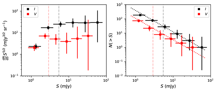
Figure 9: Differential (left) and cumulative (right) source counts for all star detections in RACS-low and VASTP-low, with Stokes $I$ and $V$ shown in black and red respectively. The red dashed line represents the RACS-low $95\text{\,}\mathrm{per~{}cent}$ completeness limit (Hale et al., 2021) which we take as an estimate of the Stokes $V$ completeness limit in our survey, and the black dashed line is the corresponding Stokes $I$ completeness limit for a median fractional polarisation of $50\text{\,}\mathrm{per~{}cent}$. Differential counts are multiplied by a $S^{5/2}$ Euclidean normalisation, and the cumulative counts are shown alongside dotted lines representing a Euclidean source distribution with power law slope of $N(>S)\propto S^{-3/2}$.

In Figure 9 we show the differential and cumulative source counts for all star detections in our sample in Stokes $I$ and $V$, with detections combined into six logarithmically spaced flux density bins between $160\text{\,}\mathrm{mJy}$. Counts in both polarisations are reduced at low flux densities due to incompleteness. RACS-low sources in Stokes $I$ have a $95\text{\,}\mathrm{per~{}cent}$ completeness limit of $2.9\text{\,}\mathrm{mJy}$ (Hale et al., 2021) which we take as an estimate of the $95\text{\,}\mathrm{per~{}cent}$ Stokes $V$ completeness limit, indicated by the dashed red line. The completeness limit in Stokes $I$ varies due to the range of fractional polarisation in our sample, so we show the limit for the median $|S_{V}|/S_{I}$ of $50\text{\,}\mathrm{per~{}cent}$ as the black dashed line. Above these thresholds the source counts are in agreement with a Euclidean source distribution, with flat slope in the normalised differential counts and cumulative counts $N(>S)\propto S^{-3/2}$. This is consistent with expectations as our sample is contained within $\sim$$500\text{\,}\mathrm{pc}$ and therefore any directional bias in counts due to Galactic plane structure is minimal (West et al., 2008).

Between RACS-low and VASTP-low our circular polarisation search has covered a total area of $135\,498\text{\,}\deg^{2}$ and resulted in 229 radio star detections, 96 of which are of M-dwarfs with the majority of detections attributable to coherent radio bursts. This corresponds to an instantaneous radio star detection surface density of $1.7\pm 0.2\times 10^{-3}$ $\text{\,}\deg^{-2}$ on $12\text{\,}\mathrm{min}$ timescales, and ${7.1}^{\thinspace+{1.6}}_{-{1.4}}\times 10^{-4}$ $\text{\,}\deg^{-2}$ considering only M-dwarf detections. The full VAST survey with ASKAP will run with similar observing parameters to VASTP-low with a plan to conduct 5953 $12\text{\,}\mathrm{min}$ observations annually, and should therefore detect ${\sim}200\pm 50$ radio stars including ${\sim}130\pm 40$ M-dwarfs each year. Scaling our measured surface densities to the expected SKA-mid $770\text{\,}\mathrm{MHz}$ 1-hour sensitivity of $4.4\text{\,}\mathrm{\SIUnitSymbolMicro Jy}\text{\,}{\mathrm{PSF}}^{-1}$ (Braun et al., 2019) and accounting for the factor of five increase in integration time, we expect a radio and M-dwarf surface density of $1.2\pm 0.3$ $\text{\,}\deg^{-2}$ and $0.7\pm 0.2$ $\text{\,}\deg^{-2}$ respectively. All-sky surveys with SKA-mid should therefore expect to detect ${41\,000}^{\thinspace+{10\,000}}_{-{9\,000}}$ radio stars, with a ${10}^{15}\text{\,}\mathrm{erg}\text{\,}{\mathrm{s}}^{-1}\text{\,}{\mathrm{Hz}}^{-1}$ completeness horizon of $\sim$$200\text{\,}\mathrm{pc}$ and ${10}^{17}\text{\,}\mathrm{erg}\text{\,}{\mathrm{s}}^{-1}\text{\,}{\mathrm{Hz}}^{-1}$ bursts detectable out to $\sim$$2\text{\,}\mathrm{kpc}$.

6 CONCLUSIONS AND OUTLOOK

As part of the ASKAP pilot survey program we have conducted a multi-epoch circular polarisation search for radio stars. Between RACS-low and VASTP-low we have made 229 detections of a sample of 76 stars, with the majority of detections attributed to coherent M-dwarf radio bursts. Through repeat observations of the VASTP-low survey footprint we constrain the typical duty cycle of radio bursts in the M-dwarf population to less than $8\text{\,}\mathrm{per~{}cent}$, and find that at least $10\pm 3$ $\mathrm{per~{}cent}$ of the population should produce bursts with a radio luminosity greater than ${10}^{13}\text{\,}\mathrm{erg}\text{\,}{\mathrm{s}}^{-1}\text{\,}{\mathrm{Hz}}^{-1}$.

Circular polarisation searches have been well demonstrated as a discovery tool for radio stars, and full ASKAP surveys will produce hundreds of new radio star detections per year helping to build larger statistical samples. The full VAST survey is underway, and with further repeat sampling we will be able to better characterise the rate and luminosity distributions of M-dwarf radio bursts and extend this analysis to other radio star classes. Repeat detections will provide insight into the range of burst parameters in individual stars and their relationship with other stellar activity parameters, such as rapid rotation, chromospheric activity, and multi-wavelength transient behaviour.

These surveys will also provide a large number of candidates for targeted followup with wide-bandwidth, high instantaneous sensitivy instruments such as the Australia Telescope Compact Array (ATCA) and MeerKAT, allowing the phenomenology of their activity to be further characterised with dynamic spectroscopy and polarimetry. Identification of the emission processes responsible for coherent stellar radio bursts will provide important insights into the magnetospheric processes present in these systems, helping to distinguish whether they more resemble the stochastic radio activity observed from the Sun, rotationally modulated pulses driven by auroral current systems, or other magnetospheric processes unobserved in the Solar system.

Data Availability

The ASKAP data analysed in this paper (RACS-low and VASTP-low) can be accessed through the CSIRO ASKAP Science Data Archive (CASDA) under project codes AS110 and AS107.

References

- Adelman-McCarthy et al. (2008) Adelman-McCarthy J. K., et al., 2008, ApJS, 175, 297
- Andrae et al. (2018) Andrae R., et al., 2018, A&A, 616, A8
- Andre (1996) Andre P., 1996, in Taylor A. R., Paredes J. M., eds, ASP Conference Series Vol. 93, Radio Emission from the Stars and the Sun. pp 273–284
- Anumarlapudi et al. (2023) Anumarlapudi A., et al., 2023, ApJ, 956, 28
- Astropy Collaboration et al. (2013) Astropy Collaboration et al., 2013, A&A, 558, A33
- Astropy Collaboration et al. (2018) Astropy Collaboration et al., 2018, AJ, 156, 123
- Bastian et al. (2022) Bastian T., Cotton W., Hallinan G., 2022, ApJ, 935, 99
- Becker et al. (1995) Becker R. H., White R. L., Helfand D. J., 1995, ApJ, 450, 559
- Bowman et al. (2013) Bowman J. D., et al., 2013, PASA, 30, 31
- Braun et al. (2019) Braun R., Bonaldi A., Bourke T., Keane E., Wagg J., 2019, arXiv e-prints
- Callingham et al. (2021a) Callingham J. R., et al., 2021a, Nature Astronomy, 5, 1233
- Callingham et al. (2021b) Callingham J. R., et al., 2021b, A&A, 648, A13
- Callingham et al. (2023) Callingham J. R., et al., 2023, A&A, 670, A124
- Chiuderi Drago & Klein (1990) Chiuderi Drago F., Klein K. L., 1990, Ap&SS, 170, 81
- Condon (1997) Condon J. J., 1997, PASP, 109, 166
- Cornwell et al. (2011) Cornwell T., Humphreys B., Lenc E., Voronkov M., Whiting M., 2011, Technical report, ATNF ASKAP memorandum 27: ASKAP Science Processing, https://www.atnf.csiro.au/projects/askap/ASKAP-SW-0020.pdf. CSIRO, https://www.atnf.csiro.au/projects/askap/ASKAP-SW-0020.pdf
- Das et al. (2022) Das B., et al., 2022, ApJ, 925, 125
- Dobie et al. (2023) Dobie D., et al., 2023, MNRAS, 519, 4684
- Duchesne et al. (2023) Duchesne S. W., et al., 2023, Publ. Astron. Soc. Australia, 40, e034
- Dulk (1985) Dulk G., 1985, ARA&A, 23, 169
- Gaia Collaboration et al. (2022) Gaia Collaboration et al., 2022, arXiv e-prints, p. arXiv:2208.00211
- Golovin et al. (2023) Golovin A., Reffert S., Just A., Jordan S., Vani A., Jahreiß H., 2023, A&A, 670, A19
- Güdel (2002) Güdel M., 2002, ARA&A, 40, 217
- Guzman et al. (2019) Guzman J., et al., 2019, ASKAPsoft: ASKAP science data processor software, astrophysics source code library, record ascl:1912.003
- Hale et al. (2021) Hale C. L., et al., 2021, PASA, 38, e058
- Hallinan et al. (2006) Hallinan G., Antonova A., Doyle J. G., Bourke S., Brisken W. F., Golden A., 2006, ApJ, 653, 690
- Hallinan et al. (2007) Hallinan G., et al., 2007, ApJ, 663, L25
- Han et al. (1998) Han J. L., Manchester R. N., Xu R. X., Qiao G. J., 1998, MNRAS, 300, 373
- Harris et al. (2020) Harris C. R., et al., 2020, Nature, 585, 357
- Helfand et al. (1999) Helfand D. J., Schnee S., Becker R. H., White R. L., McMahon R. G., 1999, AJ, 117, 1568
- Hotan et al. (2014) Hotan A., et al., 2014, PASA, 31, E041
- Hotan et al. (2021) Hotan A., et al., 2021, PASA, 38, e009
- Hunter (2007) Hunter J. D., 2007, Computing In Science & Engineering, 9, 90
- Johnston & Kerr (2018) Johnston S., Kerr M., 2018, MNRAS, 474, 4629
- Johnston et al. (2008) Johnston S., et al., 2008, Experimental Astronomy, 22, 151
- Kao et al. (2016) Kao M. M., Hallinan G., Pineda J. S., Escala I., Burgasser A., Bourke S., Stevenson D., 2016, ApJ, 818, 24
- Kao et al. (2018) Kao M. M., Hallinan G., Pineda J. S., Stevenson D., Burgasser A., 2018, The Astrophysical Journal Supplement Series, 237, 25
- Kimball et al. (2009) Kimball A. E., Knapp G. R., Ivezić E., West A. A., Bochanski J. J., Plotkin R. M., Gordon M. S., 2009, ApJ, 701, 535
- Lenc et al. (2018) Lenc E., Murphy T., Lynch C. R., Kaplan D. L., Zhang S. N., 2018, MNRAS, 478, 2835
- Lynch et al. (2015) Lynch C., Mutel R. L., Güdel M., 2015, ApJ, 802, 106
- Macquart (2002) Macquart J.-P., 2002, PASA, 19, 43
- Matthews (2019) Matthews L. D., 2019, PASP, 131, 016001
- McConnell et al. (2016) McConnell D., et al., 2016, PASA, 33, E042
- McConnell et al. (2020) McConnell D., et al., 2020, PASA, 37, e048
- McKinney (2011) McKinney W., 2011, Python for High Performance and Scientific Computing, 14
- Morris & Mutel (1988) Morris D. H., Mutel R. L., 1988, AJ, 95, 204
- Murphy et al. (2021) Murphy T., et al., 2021, PASA, 38, e054
- Nichols et al. (2012) Nichols J. D., Burleigh M. R., Casewell S. L., Cowley S. W. H., Wynn G. A., Clarke J. T., West A. A., 2012, ApJ, 760, 59
- Pritchard et al. (2021) Pritchard J., et al., 2021, MNRAS, 502, 5438
- Robishaw & Heiles (2018) Robishaw T., Heiles C., 2018, arXiv e-prints, p. arXiv:1806.07391
- Rose et al. (2023) Rose K., et al., 2023, ApJ, 951, L43
- Route & Wolszczan (2012) Route M., Wolszczan A., 2012, ApJ, 747, L22
- Shimwell et al. (2017) Shimwell T., et al., 2017, A&A, 598, A104
- Slee et al. (1987) Slee O. B., Nelson G. J., Stewart R. T., Wright A. E., Innis J. L., Ryan S. G., Vaughan A. E., 1987, MNRAS, 229, 659
- Slee et al. (2008) Slee O. B., Wilson W., Ramsay G., 2008, PASA, 25, 94
- Toet et al. (2021) Toet S. E. B., Vedantham H. K., Callingham J. R., Veken K. C., Shimwell T. W., Zarka P., Röttgering H. J. A., Drabent A., 2021, A&A, 654, A21
- Treumann (2006) Treumann R. A., 2006, A&ARv, 13, 229
- Trigilio et al. (2000) Trigilio C., Leto P., Leone F., Umana G., Buemi C., 2000, A&A, 362, 281
- Van Der Walt et al. (2011) Van Der Walt S., Colbert S. C., Varoquaux G., 2011, Computing in Science & Engineering, 13, 22
- Vedantham et al. (2020a) Vedantham H. K., et al., 2020a, Nature Astronomy, 4, 577
- Vedantham et al. (2020b) Vedantham H. K., et al., 2020b, ApJ, 903, L33
- Vedantham et al. (2023) Vedantham H. K., et al., 2023, arXiv e-prints, p. arXiv:2301.01003
- Vidotto et al. (2012) Vidotto A. A., Fares R., Jardine M., Donati J. F., Opher M., Moutou C., Catala C., Gombosi T. I., 2012, MNRAS, 423, 3285
- Villadsen & Hallinan (2019) Villadsen J., Hallinan G., 2019, ApJ, 871, 214
- Wang et al. (2021) Wang Z., et al., 2021, ApJ, 920, 45
- Wang et al. (2022) Wang Y., et al., 2022, ApJ, 930, 38
- Wes McKinney (2010) Wes McKinney 2010, in Stéfan van der Walt Jarrod Millman eds, Proceedings of the 9th Python in Science Conference. pp 56–61, doi:10.25080/Majora-92bf1922-00a, https://doi.org/10.25080/Majora-92bf1922-00a
- West et al. (2008) West A. A., Hawley S. L., Bochanski J. J., Covey K. R., Reid I. N., Dhital S., Hilton E. J., Masuda M., 2008, AJ, 135, 785
- White & Franciosini (1995) White S. M., Franciosini E., 1995, ApJ, 444, 342
- White et al. (1989) White S. M., Jackson P. D., Kundu M. R., 1989, ApJS, 71, 895
- Whiting & Humphreys (2012) Whiting M., Humphreys B., 2012, PASA, 29, 371
- Williams & Berger (2015) Williams P. K. G., Berger E., 2015, ApJ, 808, 189
- Zic et al. (2019) Zic A., et al., 2019, MNRAS, 488, 559
- Zic et al. (2020) Zic A., et al., 2020, ApJ, 905, 23
- van Haarlem et al. (2013) van Haarlem M. P., et al., 2013, A&A, 556, A2