Predicting depinning dynamics of elastic interfaces by machine learning

Abstract

Predicting the future behaviour of complex systems exhibiting critical-like dynamics is often considered to be an intrinsically hard task. Here, we study the predictability of the depinning dynamics of elastic interfaces in random media driven by a slowly increasing external force, a paradigmatic complex system exhibiting critical avalanche dynamics linked to a continuous non-equilibrium depinning phase transition. To this end, we train a variety of machine learning models to infer the mapping from features of the initial relaxed line shape and the random pinning landscape to predict the sample-dependent staircase-like force-displacement curve that emerges from the depinning process. Even if for a given realization of the quenched random medium the dynamics are in principle deterministic, we find that there is an exponential decay of the predictability with the displacement of the line, quantifying how the system forgets its initial state as it nears the depinning transition from below. Our analysis on how the related displacement scale depends on the system size and the dimensionality of the input descriptor reveals that the onset of the depinning phase transition gives rise to fundamental limits to predictability.

I Introduction

From predicting tipping points in ecosystems by monitoring their loss of resilience [1, 2] to forecasting earthquakes by measuring subtle precursory seismic signals [3], the pursuit of forecasting the future behaviour of complex systems [4, 5] is a fascinating endeavour which, if successful, would be extremely useful. Yet, attempts of this kind have typically resulted in partial success only, and the prediction accuracy of, e.g., the occurrence time and magnitude of the next earthquake within a given region has not reached levels needed to make the predictions to be of much practical utility [6]. While it is qualitatively rather obvious that complex systems are by nature difficult to predict due to the non-linear nature of their collective dynamics, what exactly is the fundamental limiting factor for their predictability in each case is often unclear.

A specific class of complex systems which are important in physics and materials science is given by elastic interfaces in quenched random media driven by an external force. They exhibit a non-equilibrium depinning phase transition between pinned and moving phases at a critical value of the external force [7, 8], emerging from the interplay between quenched disorder of the medium, elasticity of the interface, and an external driving force. Examples include domain walls in ferromagnets [9] and ferroelectrics [10], contact lines in wetting [11], crack fronts in disordered solids [12], and dislocations in crystals [13]. Such systems belong to an even broader class of complex interacting systems driven out of equilibrium by external perturbations which exhibit jerky avalanche dynamics as a response, ranging from earthquakes [14] (as well as their lab-scale counterparts [15]) to materials deformation [16, 17, 18, 19, 20, 21] and fracture [22, 23] to neuronal [24, 25] and financial avalanches [26]. The avalanches typically follow broad, power-law size distributions and obey universal scaling laws [27], in analogy to scale-free features observed at equilibrium continuous phase transitions.

Due to the critical dynamics of the depinning phase transition, manifested as avalanches with a power-law size distribution characterized by power law exponents that derive from the depinning transition critical point, predicting the time-evolution of the interface in the proximity of the critical external force value is expected to be an inherently hard task [28]: The critical avalanches are by nature expected to be always on the edge of stopping while propagating. Therefore, for instance whether a given avalanche will become large or small is expected to be governed by small fluctuations that should be hard if not impossible to predict. Thus, it is typically implicitly assumed that a probabilistic description in terms of avalanche size distributions and related statistical quantities is, at least from a practical perspective, the best possible description of such complex systems.

On the other hand, for zero temperature and for a given realization of the quenched random medium, the dynamics of the interface are deterministic within simple models such as the quenched Edwards-Wilkinson (qEW) equation [29, 30], a paradigmatic model of driven elastic interfaces in random media we study in this work. Hence, given a (coarse-grained) description of the relaxed initial state of the interface as well as that of the quenched random medium, one might expect some degree of predictability of the ensuing depinning dynamics. The key questions then are how good this predictability is, and if perfect predictions cannot be established, what are the factors limiting it?

Here, we address these questions by training machine learning (ML) models to infer the mapping from features of the initial, relaxed line configuration and the quenched random medium to the force-displacement curve characterizing the transient approach towards the depinning transition from below. The quality of predictions produced by the ML models (quantified by the coefficient of determination, $R^{2}$, between predicted and real values) is a useful measure of predictability as the ML models are not biased or limited by human ”physical intuition”. In this work, we employ different ML models ranging from linear regression to neural networks to convolutional neural networks, considering both one and two-dimensional (1D and 2D, respectively) input fields. This approach has parallels to recent studies aiming at predicting the plastic deformation process of crystals subject to applied stresses [31, 32, 33], a complex problem which in the absence of static obstacles to dislocation motion (e.g., precipitates) is controlled by dislocation jamming [34], resulting in an ”extended critical” phase without a well-defined critical point [35, 36]. Here, the physical system we consider exhibits different dynamics that are controlled by the presence of a non-equilibrium phase transition critical point with well-known properties [37], thus potentially allowing for a more clear-cut interpretation of the results concerning predictability. Indeed, a somewhat analogous problem is given by predicting the depinning dynamics of a dislocation pileup in a random quenched pinning potential [38], with the important difference that in the present case the elastic line is moving in a direction perpendicular to the average line orientation, thus always meeting new, previously unseen disorder as it propagates forward.

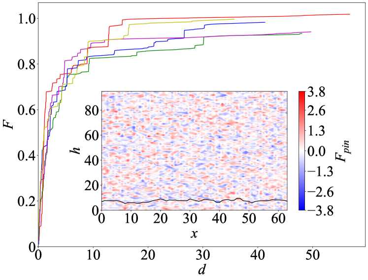
Figure 1: Main figure: Examples of force-displacement curves $F(d)$ for different realizations of the random pinning field $F_{\textrm{pin}}(x,h)$. Inset: An example of the relaxed line profile $h(x)$ (black line) and the corresponding quenched pinning field $F_{\textrm{pin}}(x,h)$ (colored according to the colorbar shown on the right). Our goal in this paper is to study to what extent the individual $F(d)$-curves can be predicted using information shown in the inset (initial line profile and the quenched pinning field).

Our results reveal an exponential decay of the predictability with the average interface displacement $d$, quantified by the coefficient of determination $R^{2}\propto\exp(-d/d_{0})$. The related displacement scale $d_{0}$ is a measure of how quickly the system loses its memory [39] of the initial interface configuration as the interface moves forward. We show that considering 1D input fields, characterizing the shape of the relaxed 1D interface and the pinning landscape only along it, leads to a shorter memory (smaller $d_{0}$) than considering 2D input fields including information of the quenched pinning field also ahead of the relaxed interface. Our main result is an intriguing size effect in the case of the 2D input fields showing that $d_{0}\propto L^{\zeta}$, with $L$ the system size and $\zeta$ the roughness exponent, suggesting that predictability of the interface dynamics is limited by the depinning phase transition the system is approaching from below. Thus, our results provide a novel, quantitative perspective on how predictability of the dynamics of a complex system is limited by the proximity of a continuous non-equilibrium phase transition.

II Methods

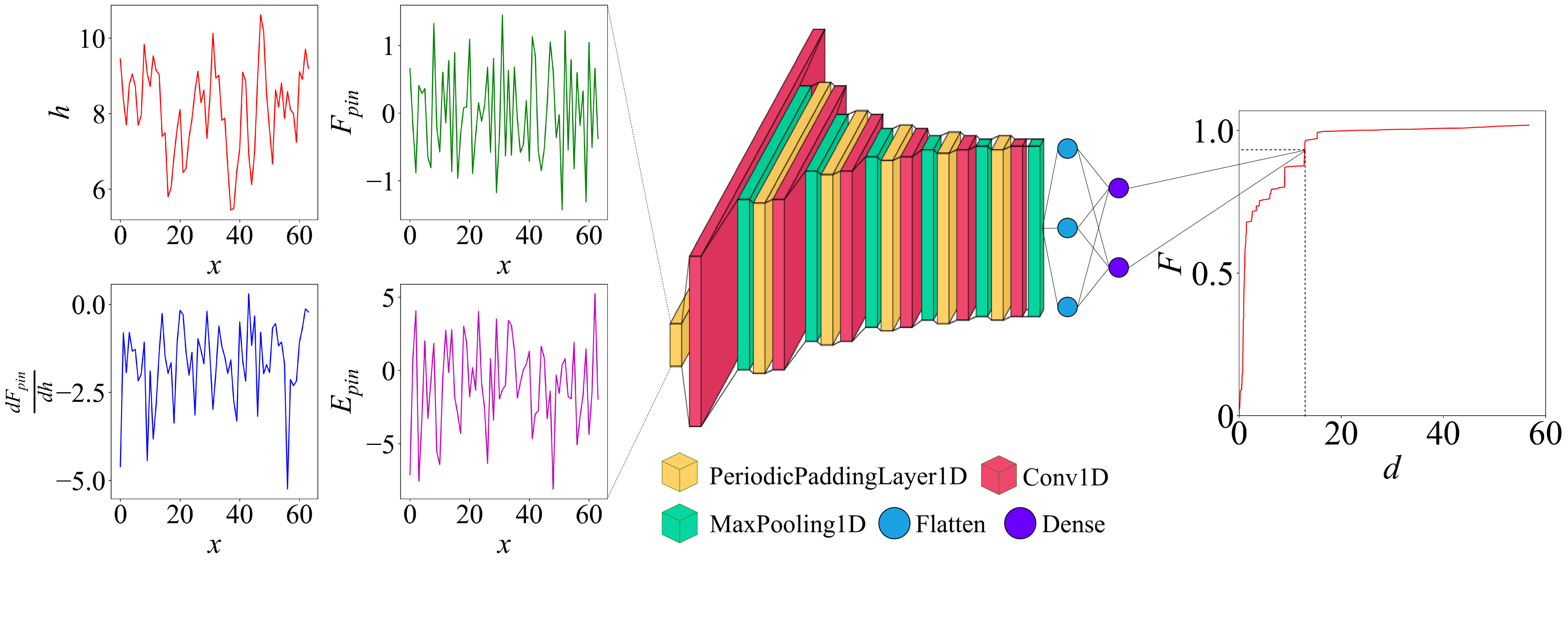
Figure 2: Schematic representation of the 1D CNN. The 1D fields along the relaxed line are fed into the CNN as the input arrays. That input is subsequently passed into padding, convolutional and pooling layers. The size of the array, represented here as its width, is reduced by half at each pooling layer until it is equal to 1. The number of parallel channels, represented by the height of the arrays, corresponds to the number of the convolutional filters. The flatten layer converts the final array of the width 1 into a linear array of the size equal to the number of filters. Finally, the dense layer gives the prediction of $F(d)$ as the output.

II.1 Quenched Edwards-Wilkinson equation

To explore the predictability of the depinning dynamics of elastic interfaces in random media, we consider as an example system the qEW equation, defined by the equations of motion

$$\frac{\partial h_{i}}{\partial t}=\Gamma_{0}\nabla^{2}h_{i}+F_{\textrm{pin}}(i,h_{i})+F$$ (1)

for the continuous variables $h_{i}$, $i=1,...,L$ (with $L$ the system size), which constitute a discretized (along the average elastic line direction) description of the interface $h(x)$. $\Gamma_{0}$ is the stiffness of the interface, $F_{\textrm{pin}}$ is a position-dependent quenched random force (i.e., it is a function of $i$ and $h_{i}$ only), and $F$ is the external driving force. We employ periodic boundary conditions along the line, and discretize the Laplacian by setting $\nabla^{2}h_{i}=h_{i+1}+h_{i-1}-2h_{i}$. The quenched disorder field $F_{\textrm{pin}}(i,h_{i})$ is constructed by first forming a regular discrete grid of size $L\times h_{\mathrm{max}}$ (with $h_{\mathrm{max}}>L$ depending on $L$; $h_{\mathrm{max}}=80$, 128 and 192 for $L=32$, 64 and 128, respectively) with unit spacing, and a random number is drawn from the standard normal distribution $N(0,1)$ to each grid point. Spline interpolation is then employed separately for each $i$ to obtain a continuous disorder field along the direction of interface motion. An example of the resulting disorder field $F_{\textrm{pin}}$ is given in the inset of Fig. 1. In the simulations, Eqs. (1) are integrated numerically using the Euler method, starting from a relaxation stage at $F=0$ from an initial height of $h_{i}=L/8$ for all $i$ (resulting in a rough line profile, see the black line in the inset of Fig. 1 for an example), after which $F$ is ramped up from zero at a slow rate of $\partial F/\partial t=0.0001$, chosen to approximate a quasistatically increasing $F$. The simulation is run until the first interface segment $i$ reaches a height close to but below the maximum allowed height of $h_{i}=h_{\mathrm{max}}$; this also roughly corresponds to the interface reaching the depinning transition at an effective $L$-dependent critical value of the external force, $F=F_{c}(L)$.

Unless stated otherwise, we consider a small system with $L=64$, which is expected to result in significant sample-to-sample variation in the response to external forces quantified by the force-displacement curve $F(d)$, where $d=\langle h_{i}(F)-h_{i}(0)\rangle_{i}$ is the $F$-dependent average interface displacement; our aim is to predict the sample-specific $F(d)$ using information of the initial configuration of the system, described by the relaxed line profile $h_{i}(0)$, $i=1,...,L$, and the quenched pinning landscape, as input. Examples of force-displacement curves $F(d)$ obtained for different realizations of the random pinning force are shown in the main figure of Fig. 1. One can observe the typical random-looking staircase-like shape of the curves, corresponding to a sequence of avalanches of interface propagation [the horizontal segments of $F(d)$, which tend to become larger upon increasing $F$] separated by the vertical segments corresponding to the external force increasing while the interface is pinned by the disorder. Due to the small system size considered, the response $F(d)$ exhibits rather pronounced sample-to-sample variations which we aim at predicting.

To compute the database used to train the ML models, for $L=64$, the simulation procedure described above is repeated for 40000 different random realization of the pinning field $F_{\textrm{pin}}(i,h_{i})$. The database then consists of the 40000 $F(d)$-curves and the corresponding descriptors of the initial relaxed configuration (see below for details on what these are for the different ML models). In order to address the question of how the system size $L$ affects predictability, we also compute two additional databases: 10000 configurations for $L=32$ and 10000 configurations for $L=128$.

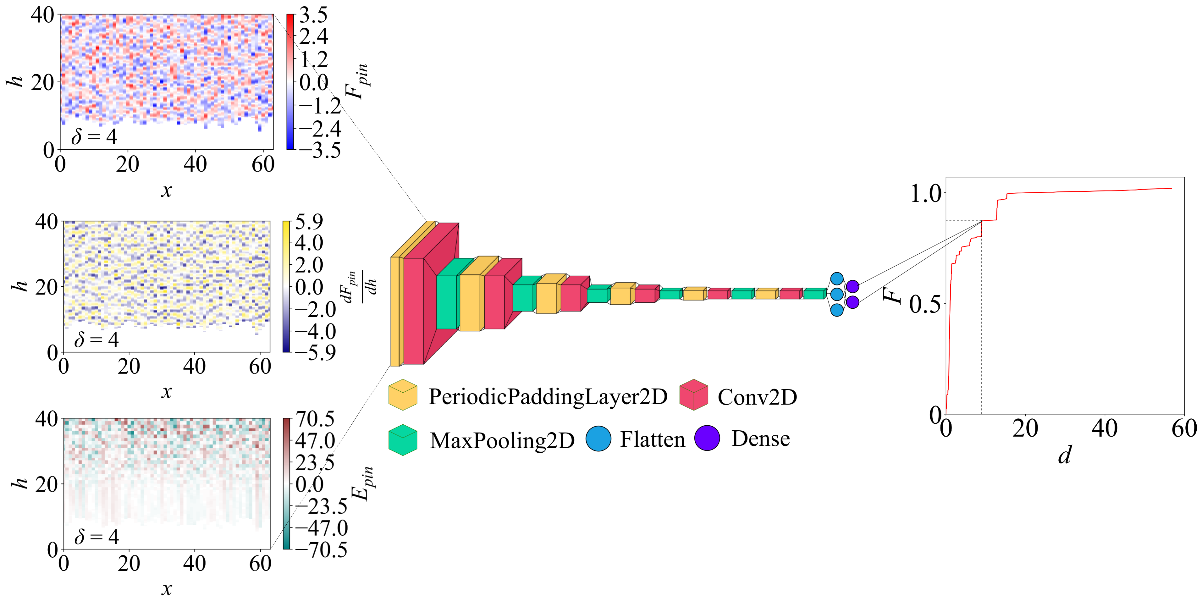
Figure 3: Schematic representation of the 2D CNN. The 2D fields $F_{\mathrm{pin}}$, $\mathrm{d}F_{\mathrm{pin}}/\mathrm{d}h$ and $E_{\mathrm{pin}}$ are fed into the CNN as the input arrays. That input is subsequently passed into padding, convolutional and pooling layers. The size of the array in the two dimensions, represented here as its width and height, is reduced by half at each pooling layer until it is equal to 1$\times$1. The number of parallel channels, represented as the thickness of the arrays, corresponds to the number of the convolutional filters. The flatten layer converts the final array of the size 1$\times$1 into a linear array of the size equal to the number of filters. Finally, the dense layer gives the prediction of $F(d)$ as the output.

II.2 Machine learning models for predictability analysis

To study the predictability of the depinning dynamics, we consider three different ML models: Linear regression (LR), fully connected neural networks (NNs) and convolutional neural networks (CNNs) [40]. Together these cover a broad range of different model types, ranging from linear mappings from user-defined features (LR, see Appendix A) to non-linear mappings without the need for feature engineering by the user (CNN). For LR and NN, the input features used are statistical properties (average, standard deviation, kurtosis, skewness, maximum, and the absolute values of the first and second Fourier coefficients along the interface) of the relaxed line profile $h(x)$, as well as of three 1D profiles measured along the relaxed line profile: the pinning force $F_{\mathrm{pin}}(x)$, its derivative $\mathrm{d}F_{\mathrm{pin}}/\mathrm{d}h(x)$, and the pinning energy $E_{\mathrm{pin}}(x)=-\int_{0}^{h(x)}F_{\mathrm{pin}}\mathrm{d}h$, see Fig. 2 and Appendix A for example profiles.

For the CNN, the input consists of 1D or 2D fields without feature engineering: The 1D fields are the ones from which the statistical features used for LR and NN are extracted (see again Fig. 2 and Appendix A). The 2D fields include information of the pinning field also ahead of the relaxed line profile, i.e., for $h>h(x)$, where $h(x)$ is the relaxed line profile; they are given by $F_{\mathrm{pin}}(x,h)$, $\mathrm{d}F_{\mathrm{pin}}/\mathrm{d}h(x,h)$ and $E_{\mathrm{pin}}(x,h)$, see Fig. 3 and Appendix A for examples. The 2D fields contain zeros below the relaxed line profile, i.e., for $h<h(x)$, and hence the interface between zeros and (mostly) non-zero values contains information of the relaxed line configuration. Thus, overall, the 1D and 2D fields contain information of the same quantities, but the 2D fields (which are given with different resolutions $\delta$) include information of the pinning field also ahead of the relaxed line profile. The resolution of these fields is such that there are always $L$ pixels in the $x$-direction, and $\delta$ (where $\delta$ defines the resolution) pixels per unit displacement in the $h$-direction. For details on the ML models and the input features used, see Appendix A.

III Results

III.1 Feature importance

In order to shed some light on which features fed to the LR and NN models are important in determining the external force value $F(d)$ for a given displacement $d$, we start by considering the linear correlations (quantified by the square of the sample correlation coefficient, $r^{2}$) between the values of the various descriptors and $F(d)$. These are shown in Fig. 4, considering separately the features extracted from $h$, $F_{\mathrm{pin}},\mathrm{d}F_{\mathrm{pin}}/\mathrm{d}h$, and $E_{\mathrm{pin}}=-\int_{0}^{h_{i}}F_{\mathrm{pin}}\mathrm{d}h$, respectively. The general observation is that most of the features are very weakly correlated with $F(d)$, and the $r^{2}$-values for those features that exhibit slightly stronger correlations clearly decay with $d$. One may note that especially for small $d$ the strongest correlations are found for the average values of $\mathrm{d}F_{\mathrm{pin}}/\mathrm{d}h$ and $h$. The former relates to the stability of the relaxed interface configuration, and the latter quantifies the drift of the interface position away from its initial position during relaxation. However, none of the features alone exhibit strong correlations, and hence we proceed to consider their combined effect by employing the ML models.

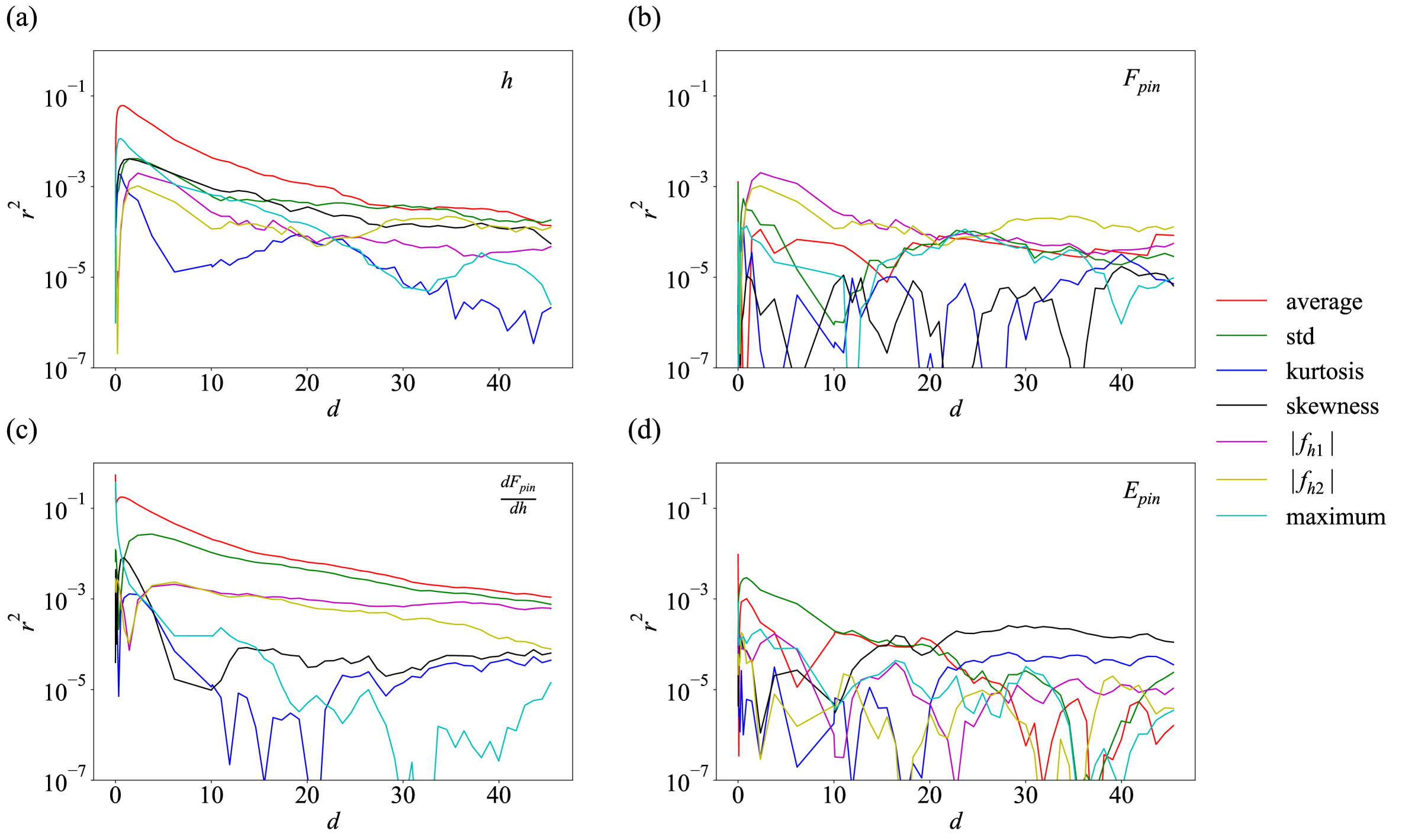
Figure 4: The square of the sample correlation coefficient $r^{2}$ of the different statistical features of the fields fed into the LR and NN models with the external driving force $F(d)$ as the function of the displacement $d$. (a) The relaxed interface profile $h$, (b) the pinning field $F_{\mathrm{pin}}$, (c) the pinning force derivative $\mathrm{d}F_{\mathrm{pin}}/\mathrm{d}h$, and (d) the pinning energy $E_{\mathrm{pin}}$.

III.2 Predictability: 1D fields

To study the overall predictability when all the different features (either 1D or 2D) are used together as input, the ML models introduced above are considered. The predictability is quantified by the coefficient of determination $R^{2}$, defined by

$$R^{2}=1-\frac{\sum_{i=1}^{N}[F_{i}^{\mathrm{true}}(d)-F_{i}^{\mathrm{pred}}(d)]^{2}}{\sum_{i=1}^{N}[F_{i}^{\mathrm{true}}(d)-\langle F_{i}^{\mathrm{true}}(d)\rangle]^{2}},$$ (2)

where $F_{i}^{\mathrm{true}}(d)$ is the true value [i.e., the value obtained from the numerical solution of Eq. (1)] of the force $F(d)$ at a specific displacement $d$ for the $i$th sample, $\langle F_{i}^{\mathrm{true}}(d)\rangle$ is its mean value, $F_{i}^{\mathrm{pred}}(d)$ is the value predicted by the ML model, and $N$ is the total number of samples in the set. $R^{2}=1$ would imply perfect predictability, while $R^{2}=0$ would mean that the model would simply predict the average response for all samples.

We start by considering predictability using the 1D input fields. We find (see Fig. 5 showing the test set $R^{2}$ for LR, NN and 1D CNN) that for $d\gtrapprox 10$ (after the small-$d$ peak for which $R^{2}$ is not much below 1), $R^{2}$ decays roughly exponentially with the displacement $d$,

$$R^{2}(d)=A\mathrm{e}^{-\left(\frac{d}{d_{0}}\right)},$$ (3)

where $d_{0}$ is the characteristic displacement scale of the exponential decay, quantifying how quickly information of the initial configuration is lost (or forgotten) with increasing $d$. For LR with $L1$ regularization, we obtain $d_{0}\approx 11$ (inset of Fig. 5). Perhaps surprisingly, NN and 1D CNN result in worse predictability for large $d$ with smaller $d_{0}$ of the exponential decay ($d_{0}\approx 6$ and $d_{0}\approx 5$ for NN and 1D CNN, respectively, see again the inset of Fig. 5). This suggests that the predictability is limited by the information content of the 1D descriptors so that increasing the complexity of the ML model (by moving from LR to NN and 1D CNN) does not improve the result but rather makes it worse for the finite training database at hand.

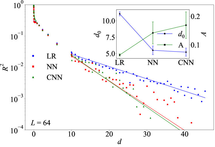
Figure 5: The coefficient of determination $R^{2}$ for the three ML models with the 1D input fields as a function of displacement $d$. Solid lines are exponential fits (Eq. 3). The inset shows the corresponding fitting parameters $d_{0}$ and $A$.

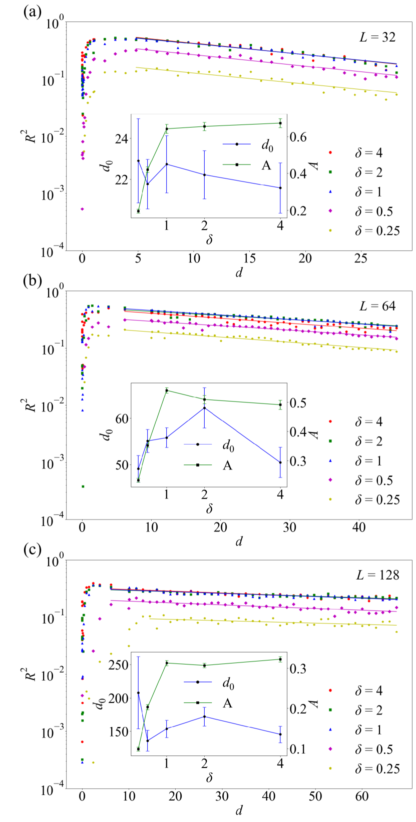
Figure 6: The coefficient of determination $R^{2}$ for the 2D CNN as a function of displacement $d$ for different system sizes $L$ [with $L=32$, 64 and 128 shown in (a), (b), and (c), respectively] and resolutions of the input $\delta$ (symbols). Lines are exponential fits [Eq. (3)]. The insets show the corresponding fitting parameters $d_{0}$ and $A$.

III.3 Predictability: 2D fields

As found above, the 1D descriptors do not contain enough information for good predictability of $F(d)$ for large $d$. This is to be expected as no information of the quenched pinning field above the relaxed interface configuration, something that to a large extent will determine the interface dynamics for $d>0$, is included in them. Therefore, we’ll consider the 2D CNN which is fed a 2D representation of the pinning field $F_{\textrm{pin}}$ ahead of the relaxed interface, together with the corresponding 2D fields of $E_{\mathrm{pin}}$ and $\mathrm{d}F_{\mathrm{pin}}/\mathrm{d}h$ (see again Fig. 3 and Appendix A).

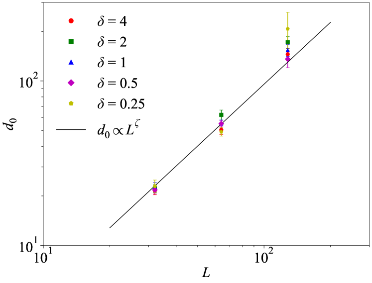
Figure 7: $d_{0}$ for the 2D CNN (from Fig. 6) as the function of the system size $L$ for different resolutions $\delta$ (symbols). Line is a fit of the form of $d_{0}\propto L^{1.25}$ [Eq. (4)].

Fig. 6 shows the resulting test set $R^{2}$ values as a function of $d$ for different resolutions $\delta$ of the pinning field descriptors, now considering three different system sizes $L$ to address the question of possible size effects in predictability. Again, an exponential decay of $R^{2}$ with $d$ [Eq. (3)] is observed for large enough $d$. We note that now $d_{0}$ is significantly larger than in the case of the 1D fields, varying between $d_{0}\approx 21$ and 23 for $L=32$, $d_{0}\approx 50$ and 60 for $L=64$, and $d_{0}\approx 140$ and 210 for $L=128$, respectively, for the different resolutions $\delta$ considered (see the insets of Fig. 6). Moreover, the exponential decay starts from a larger $R^{2}$-value for small $d$ than in the case of the 1D input fields, and hence the large-$d$ predictability (while not great) is now much better than when considering 1D input fields. One may also notice that both $d_{0}$ and the prefactor $A$ depend on $\delta$ (see again the inset of Fig. 6), such that overall the best predictability is obtained for $\delta=1$ or higher. This makes sense as $\delta=1$ matches the resolution (or density) of discrete random numbers from which the continuous $F_{\textrm{pin}}$ field is obtained via spline interpolation. Thus, for $\delta=1$ all the information of $F_{\textrm{pin}}$ is contained in the descriptor, but at the same time the number of pixels is not unnecessarily large so that the 2D CNN remains not too complex, something that helps to avoid overfitting.

The above results show that for the 2D input fields, the CNN predictability and especially the $d_{0}$-value depends on $L$, such that the exponential decay of $R^{2}$ with $d$ is slower for larger $L$. Fig. 7 shows the $d_{0}$-values for different $\delta$ as a function of $L$. The data seems to be, within error bars, consistent with the scaling with the roughness exponent $\zeta\approx 1.25$ [41, 37], i.e.,

$$d_{0}\propto L^{\zeta}.$$ (4)

When approaching the depinning transition from below starting from a flat initial configuration, one expects that the growing roughness $W$ of the interface is linked to its average height (here, the interface displacement $d$) via $W\propto d\propto\xi_{x}^{\zeta}$ (with $\xi_{x}$ the correlation length along the interface), so that the displacement $d^{*}$ at which the saturated roughness is reached at the depinning critical point (as $\xi_{x}\rightarrow L$) scales as $d^{*}\propto L^{\zeta}$. Thus, the observation that $d_{0}\propto L^{\zeta}\propto d^{*}$ [Eq. (4)] suggests that displacements $d$ up to which meaningful prediction can be made (quantified by the $d_{0}$-value) are limited by the displacement corresponding to the saturated roughness at the finite-$L$ depinning threshold. In other words, predictability is limited by the depinning phase transition from a pinned to a moving phase the system is approaching from the pinned phase. Interestingly, this scaling would indicate that since $\zeta>1$, $d_{0}/L\propto L^{\zeta-1}$ would diverge in the thermodynamic limit $L\rightarrow\infty$ for the qEW equation studied here. One may note that the prefactor $A$ has the opposite trend with $L$ (see again the insets of Fig. 6), possibly because larger $L$ implies a more complex CNN with more trainable parameters negatively affecting the learning for a database of a finite size. Notice however that the $L$ dependence of $A$ is much weaker than that of $d_{0}$: in the range of $L$-values considered, $A$ changes by a factor of $\sim 2$, while $d_{0}$ changes by almost an order of magnitude. Assuming that these trends persist for a broader range of $L$-values, this would imply that for a given large enough displacement $d$, $R^{2}$ would be larger in a system with a larger $L$.

IV Discussion and conclusions

To conclude, we have found an exponential decay with the displacement $d$ of the predictability (quantified by the coefficient of determination, $R^{2}$) of the depinning dynamics of elastic interfaces in quenched random media. The amplitude $A$ and the characteristic scale $d_{0}$ of the exponential decay are found to depend on whether the input field is 1D or 2D. The observation that the best result is obtained by using the 2D CNN highlights the crucial role of features of the sample-specific pinning field ahead of the relaxed interface configuration, in addition to the relaxed line profile. The exponential decay of $R^{2}(d)$ can be thought of as a manifestation of the system losing its memory of the initial configuration around the characteristic displacement $d_{0}$. This behaviour is in contrast with findings from analogous studies of other complex avalanching systems including 2D discrete dislocation dynamics (DDD) [31] and dislocation pileups [38], where a non-monotonic dependence of $R^{2}$ on strain has been found. This is likely due to the presence of features that are conserved during the dynamics in those systems (the 1st Fourier coefficient of the geometrically necessary dislocation density in the direction perpendicular to the dislocation motion in 2D DDD [31], and the repeated sampling of the same pinning field by the dislocation pileup with periodic boundary conditions [38]) that are absent in the present case.

Our main result, obtained by studying the size dependence of predictability, reveals that the onset of critical dynamics due to the depinning phase transition the system is approaching from below is the limiting factor for the interface displacements up to which meaningful predictions of its dynamics can be made. It is important to emphasize that this limitation to predictability emerges even in cases such as ours where the interface dynamics, for a given realization of the quenched random medium, is governed by deterministic equations of motion. This provides an interesting perspective to understand the limits of predictability in a broad range of complex systems exhibiting a continuous non-equilibrium phase transition. For the specific case at hand, i.e., the qEW equation, the observed scaling $d_{0}\propto L^{\zeta}$ together with the super-rough nature of the interface ($\zeta\approx 1.25>1$) implies that $d_{0}/L$ increases with $L$. For other elastic interfaces (such as the long-range elastic string [42, 12]) with $\zeta<1$, we hence expect $d_{0}/L$ to decrease with $L$, suggesting that predicting the large-displacement dynamics of long interfaces would be harder than in the present case. Indeed, it would be interesting to extend the present study by testing our ideas in the context of depinning of driven elastic interfaces in random media in higher dimensions (2D elastic membranes in 3D quenched random media [9]) and with other types of elasticity, including long-range and non-linear elasticity (i.e., the Kardar-Parisi-Zhang equation [29] with quenched noise). Moreover, here the initial states have been prepared by relaxation from a flat configuration at $F=0$, but one could also create them by first quasistatically ramping up the force followed by a relaxation at zero force (in analogy with the pre-strained dislocation configurations studied in Ref. [31]), thus allowing one to study possible history dependence of predictability.

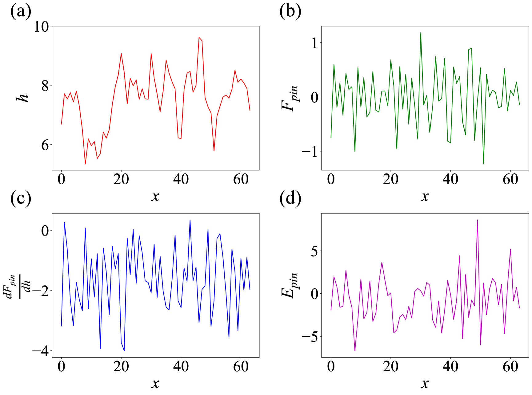
Figure 8: Examples of the 1D fields along the relaxed line configuration: (a) Line profile $h(x)$, (b) pinning force $F_{\mathrm{pin}}$, (c) first derivative of the pinning force field in the direction of interface motion $dF_{\mathrm{pin}}/dh$, and (d) the pinning potential energy $E_{\mathrm{pin}}$.

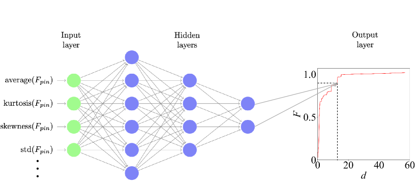
Figure 9: Schematic representation of the architecture of the NN. The statistical features of the 1D fields shown in Fig. 8 are fed as the input shown here as the green circles. They are subsequently passed forward to the hidden layers, whose neurons are represented by the blue circles. Finally, in the output layer the predicted value of $F(d)$ is obtained.

Appendix A: Details of the machine learning models

1 Linear regression

LR is the simplest predictive model utilized in this work. As its name suggests it assumes a linear dependence of the predicted value, in this case $F(d)$, on some input features $x_{i}$, which can be written as

$$F(d)=\sum_{i=1}^{N_{in}}a_{i}x_{i}+b,$$ (5)

where $N_{in}$ is the total number of the input features, while $a_{i}$ and $b$ are the coefficients that need to be fitted.

As the input features for LR various statistical descriptors (average, kurtosis, skewness, standard deviation, etc.) were extracted from the 1D fields along the relaxed line configuration ($h$, $F_{\mathrm{pin}},\mathrm{d}F_{\mathrm{pin}}/\mathrm{d}h$, and the pinning energy $E_{\mathrm{pin}}=-\int_{0}^{h_{i}}F_{\mathrm{pin}}\mathrm{d}h$; examples are shown in Fig. 8). The fitting is done by using the least squares method. In addition, L1 regularization (Lasso), which adds a penalty term to the loss function that is optimized to reduce overfitting, is applied with the factor $\lambda=10^{-3}$. The whole dataset of configurations is split into the training and test set with the ratio 80:20 %.

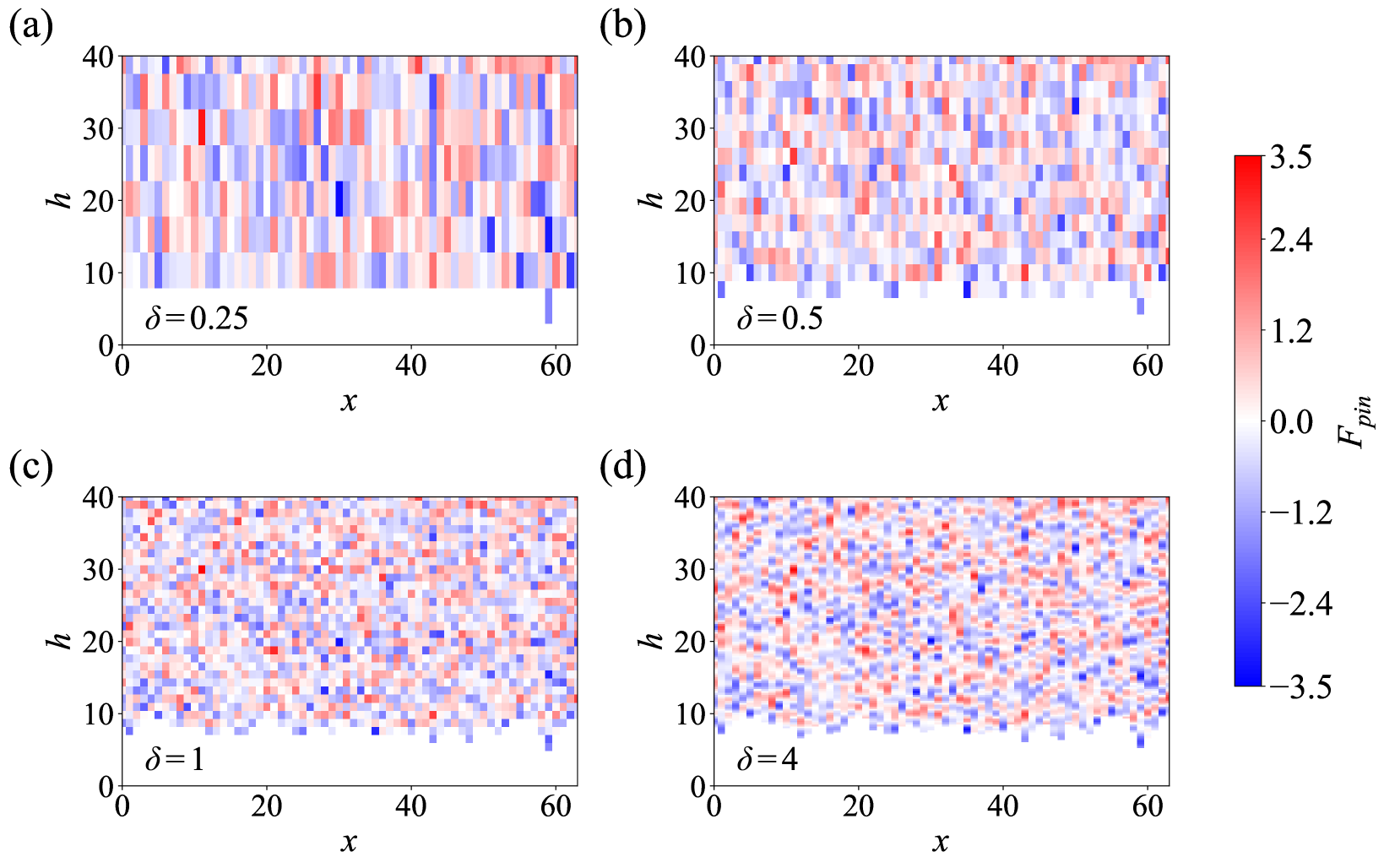
Figure 10: Examples of the two-dimensional fields of the pinning force $F_{\mathrm{pin}}$ above the relaxed line profile for different resolutions $\delta$ in the $h$-direction. (a) $\delta=0.25$, (b) $\delta=0.5$, (c) $\delta=1$, and (d) $\delta=4$.

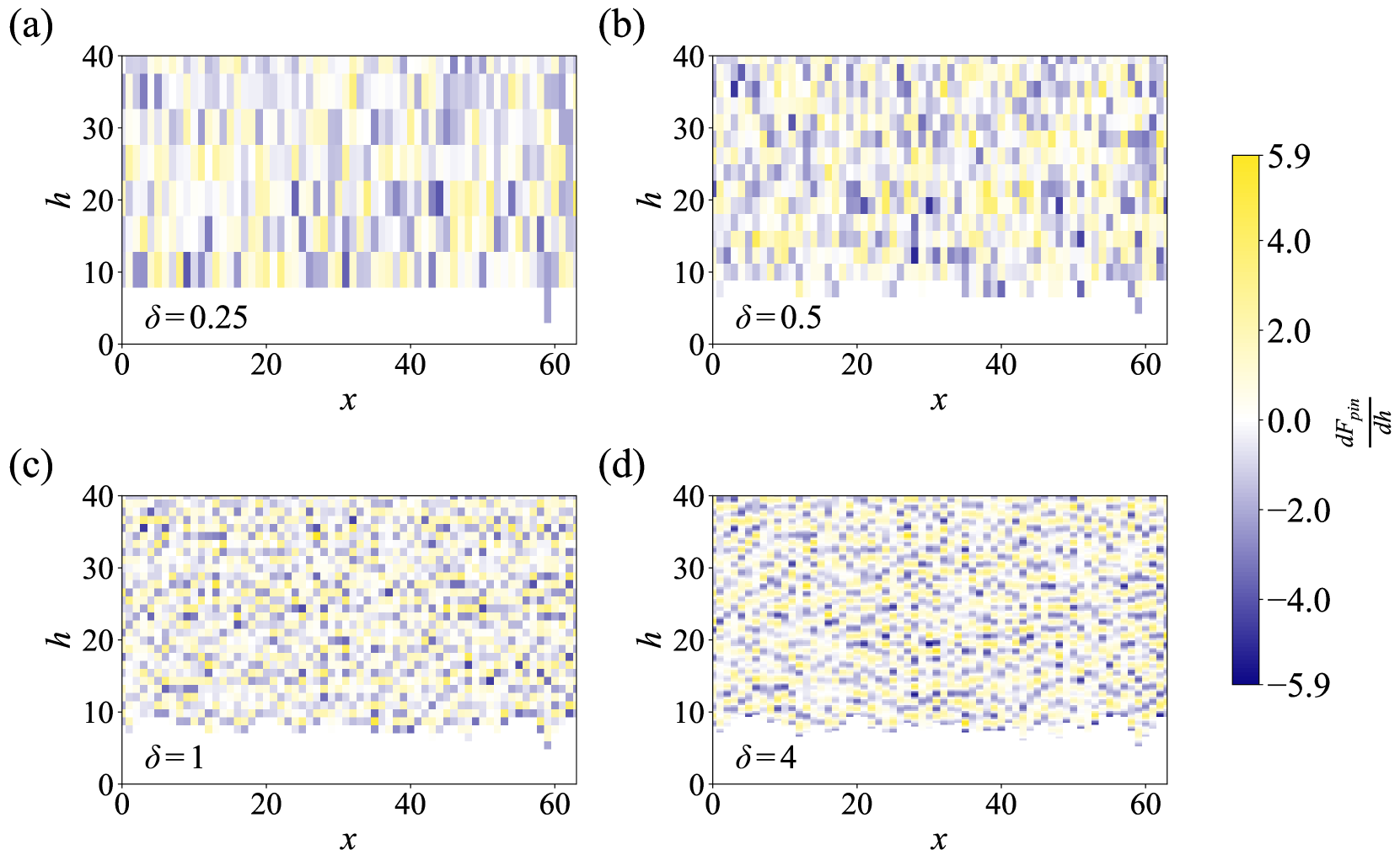
Figure 11: Examples of the two-dimensional fields of the pinning force derivative $\mathrm{d}F_{\mathrm{pin}}/\mathrm{d}h$ above the relaxed line profile for different resolutions $\delta$ in the $h$-direction. (a) $\delta=0.25$, (b) $\delta=0.5$, (c) $\delta=1$, and (d) $\delta=4$.

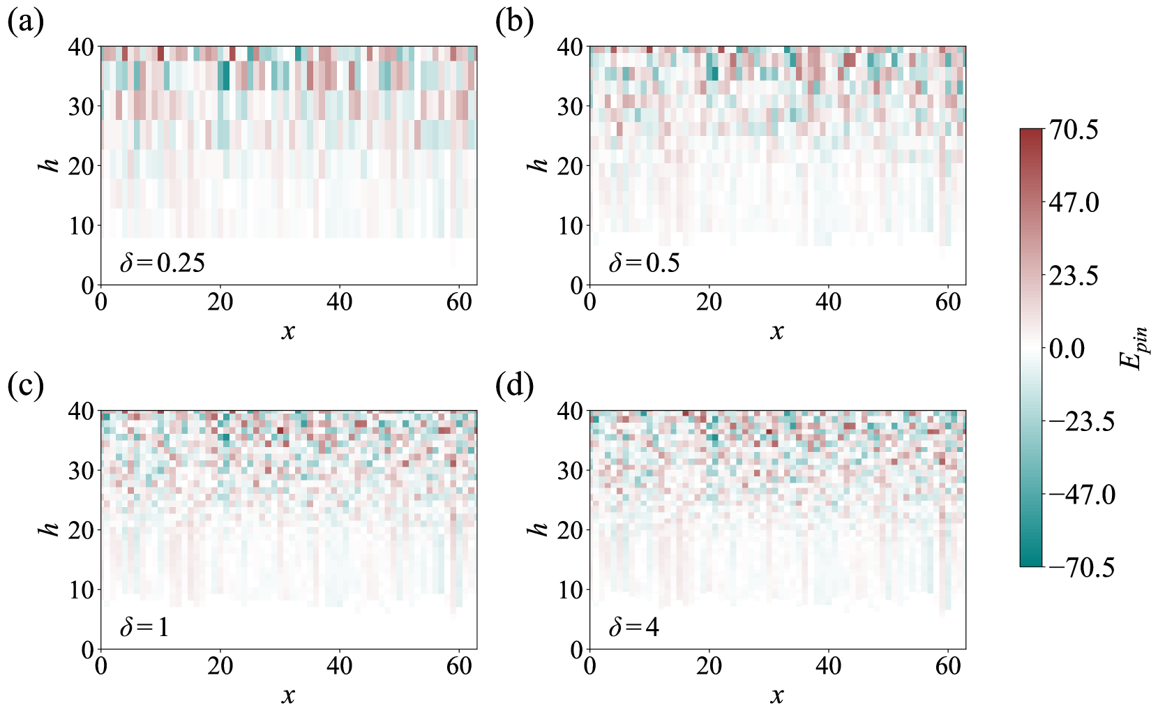
Figure 12: Examples of the two-dimensional fields of the pinning energy $E_{\mathrm{pin}}$ above the relaxed line profile for different resolutions $\delta$ in the $h$-direction. (a) $\delta=0.25$, (b) $\delta=0.5$, (c) $\delta=1$, and (d) $\delta=4$.

2 Fully connected neural network

NN being a more complex model allows to infer a non-linear relation between the input and the output. The architecture of the NN is shown schematically in Fig. 9. It consists of an input layer to which the same statistical features of the 1D input fields as those used above for LR are fed, as well as three hidden layers, and an output layer. The features are passed forward from the input layer to the subsequent hidden layers through activation functions, which are all taken to be rectifiers (ReLu). Each hidden layer consists of a certain number of neurons: Starting from the first hidden layer, the hidden layers contain 64, 16 and 4 neurons, respectively. The value in the output layer, which is the predicted value of $F(d)$, is a linear function of the values of the neurons in the last hidden layer. If one denotes the value of the $m$th neuron in the $n$th layer as $y_{m}^{n}$, then

$$y_{m}^{n}=f_{a}^{n-1}\left(w_{0m}^{n-1}+\sum_{i=1}^{N_{n-1}}w_{im}^{n-1}y_{i}^{n-1}\right),$$ (6)

where $f_{a}^{n-1}$ is the activation function between the $(n-1)$th and the $n$th layer, $N_{n-1}$ is the number of nodes in the $(n-1)$th layer and $w_{im}^{n-1}$ are the trainable parameters of the NN (called weights for $i\neq 0$ and biases for $i=0$). In the present case, if one uses 0 as the index of the input layer, $y_{m}^{0}=x_{m}$, $N_{0}=N_{in}$ and $y_{0}^{4}=F(d)$.

For the training of the NN Adam optimizer is used with the learning rate $\eta=10^{-3}$. The training lasts maximally for 1000 epochs. In addition to the training and the test set also a validation set is used, such that their ratio is 80:10:10%. The role of the validation set is to interrupt the training if its loss function (mean squared error) does not decrease for 10 consecutive epochs. L2 regularization (Ridge) is applied during the training with $\lambda=10^{-3}$.

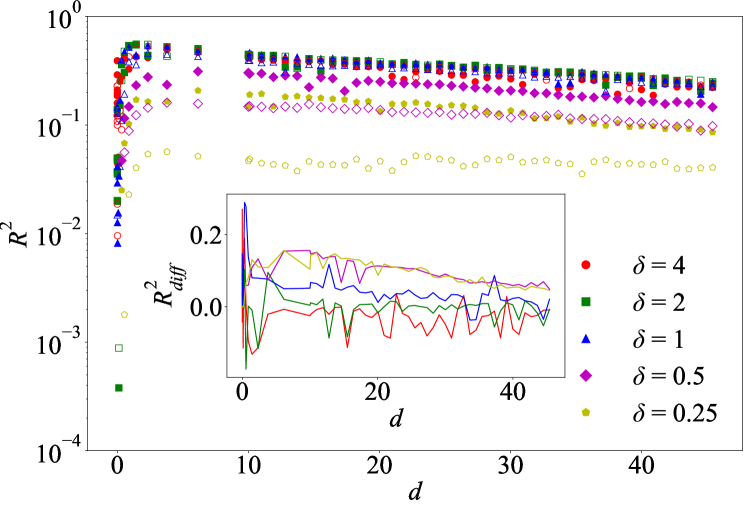
Figure 13: A comparison of $R^{2}$ vs $d$ for $L=64$ considering different resolutions $\delta$ when feeding the 2D CNN either all three fields ($F_{\mathrm{pin}}$, $\mathrm{d}F_{\mathrm{pin}}/\mathrm{d}h$ and $E_{\mathrm{pin}}$; filled symbols) or just the $F_{\mathrm{pin}}$ field (open symbols). The inset shows the difference $R^{2}_{\mathrm{diff}}=R^{2}_{\mathrm{all}}-R^{2}_{F_{\mathrm{pin}}}$ as a function of $d$ for the different $\delta$-values, with the latter indicated by the color according to the legend of the main figure.

3 Convolutional neural network

Unlike LR and NN, the CNN does not utilize the manually defined features but instead takes a pixelized image of some field describing the system as the input. That image is stored in an array of the size corresponding to its resolution and subsequently processed by several repetitions of periodic padding, convolutional and pooling layers. The periodic padding layer extends the size of the array by 2 in each direction according to periodic boundary conditions. This guarantees that the array has the same size after the convolutional layer as it had before the padding layer. Convolutional layers contain convolutional filters, whose parameters act as weights and biases (analogously to the NN) for the values from the previous layer and are adjusted during the training. In each convolutional layer there are 16 filters with the kernel size of 3 and 3$\times$3 for the 1D CNN and 2D CNN, respectively. Max-pooling layers reduce the size of the array by half. Therefore, the total number of the layers is such that the size in one or both of the dimensions is eventually reduced to 1. Behind the last pooling layer a flatten layer is inserted, which converts the array to a linear one and finally a dense layer is added with the linear activation function, which gives a prediction of $F(d)$ as the output.

We consider two types of CNNs to predict the response of the elastic line: (i) A 1D CNN where the input fields are again given by $h$, $F_{\mathrm{pin}},\mathrm{d}F_{\mathrm{pin}}/\mathrm{d}h$, and the pinning energy $E_{\mathrm{pin}}=-\int_{0}^{h_{i}}F_{\mathrm{pin}}\mathrm{d}h$, but instead of manually extracting statistical features from them, the full 1D fields are used as input, see Fig. 2 for a schematic representation of the 1D CNN. (ii) A 2D CNN where two-dimensional maps of $F_{\mathrm{pin}}$, $\mathrm{d}F_{\mathrm{pin}}/\mathrm{d}h$ and $E_{\mathrm{pin}}$ above the relaxed line profile (i.e., in the direction where the line will move once $F$ is increased from zero) are used as input. Below the relaxed line profile, the maps contain zeros, and hence the interface between zeros and (mostly) non-zero values contains information of the relaxed interface configuration. The resolution of these maps is such that there are always $L$ pixels in the $x$-direction, and $\delta$ (where $\delta$ defines the resolution) pixels per unit displacement in the $h$-direction, see Figs. 10, 11, and 12 for examples of these maps with four different resolutions $\delta$. A schematic representation of the 2D CNN is shown in Fig. 3.

As in the case of NN, the Adam optimizer is used for the CNN training with the learning rate $\eta=10^{-3}$ for $L=32$ and $L=64$, and $\eta=10^{-4}$ for $L=128$ (a smaller learning rate was needed for the training to converge for the larger system size). The maximal number of epochs is 1000 and the ratio of the training, test and validation set is again 80:10:10%. L2 regularization is applied with $\lambda=10^{-3}$.

Appendix B: Importance of the 2D input fields

In our 2D CNN analysis, we used three 2D input fields: $F_{\mathrm{pin}}$, $\mathrm{d}F_{\mathrm{pin}}/\mathrm{d}h$ and $E_{\mathrm{pin}}$. Since the latter two are in principle derivable from the first, we address here the question of how much the predictions improve as a result of feeding the 2D CNN these three fields instead of just $F_{\mathrm{pin}}$. Fig. 13 shows the $R^{2}$ vs $d$ curves as predicted by the 2D CNN for the different resolutions $\delta$ in the two cases (three vs one input field). The conclusion is that including all the three fields clearly improves $R^{2}$ for $\delta<1$, and slighly improves it for $\delta=1$ (see the inset of Fig. 13) However, for $\delta>1$, the $R^{2}$-values obtained when using the three input fields are indistinguishable from those obtained for $F_{\mathrm{pin}}$ only within statistical fluctuations. This suggests that the $E_{\mathrm{pin}}$ and $\mathrm{d}F_{\mathrm{pin}}/\mathrm{d}h$ fields are important in determining the $F(d)$ curve, but the CNN is able to figure them out from the $F_{\mathrm{pin}}$ data (by integration and differentiation of $F_{\mathrm{pin}}$, respectively) if $F_{\mathrm{pin}}$ is given with a high enough resolution such that no information of the non-interpolated random forces is lost.

References

- Dai et al. [2012] L. Dai, D. Vorselen, K. S. Korolev, and J. Gore, Generic indicators for loss of resilience before a tipping point leading to population collapse, Science 336, 1175 (2012).
- Scheffer et al. [2001] M. Scheffer, S. Carpenter, J. A. Foley, C. Folke, and B. Walker, Catastrophic shifts in ecosystems, Nature 413, 591 (2001).
- Bletery and Nocquet [2023] Q. Bletery and J.-M. Nocquet, The precursory phase of large earthquakes, Science 381, 297 (2023).
- Vlachas et al. [2022] P. R. Vlachas, G. Arampatzis, C. Uhler, and P. Koumoutsakos, Multiscale simulations of complex systems by learning their effective dynamics, Nature Machine Intelligence 4, 359 (2022).
- Craig et al. [2001] P. S. Craig, M. Goldstein, J. C. Rougier, and A. H. Seheult, Bayesian forecasting for complex systems using computer simulators, Journal of the American Statistical Association 96, 717 (2001).
- Kagan and Jackson [2000] Y. Y. Kagan and D. D. Jackson, Probabilistic forecasting of earthquakes, Geophysical Journal International 143, 438 (2000).
- Chauve et al. [2000] P. Chauve, T. Giamarchi, and P. Le Doussal, Creep and depinning in disordered media, Physical Review B 62, 6241 (2000).
- Nattermann et al. [1992] T. Nattermann, S. Stepanow, L.-H. Tang, and H. Leschhorn, Dynamics of interface depinning in a disordered medium, Journal de Physique II 2, 1483 (1992).
- Zapperi et al. [1998] S. Zapperi, P. Cizeau, G. Durin, and H. E. Stanley, Dynamics of a ferromagnetic domain wall: Avalanches, depinning transition, and the barkhausen effect, Physical Review B 58, 6353 (1998).
- Paruch et al. [2005] P. Paruch, T. Giamarchi, and J.-M. Triscone, Domain wall roughness in epitaxial ferroelectric thin films, Physical Review Letters 94, 197601 (2005).
- Joanny and De Gennes [1984] J. Joanny and P.-G. De Gennes, A model for contact angle hysteresis, Journal of Chemical Physics 81, 552 (1984).
- Laurson et al. [2013] L. Laurson, X. Illa, S. Santucci, K. T. Tallakstad, K. J. Måløy, and M. J. Alava, Evolution of the average avalanche shape with the universality class, Nature Communications 4, 1 (2013).
- Zapperi and Zaiser [2001] S. Zapperi and M. Zaiser, Depinning of a dislocation: the influence of long-range interactions, Materials Science and Engineering: A 309, 348 (2001).
- Richter and Gutenberg [1956] C. Richter and B. Gutenberg, Magnitude and energy of earthquakes, Annals of Geophysics 9, 1 (1956).
- Laurenti et al. [2022] L. Laurenti, E. Tinti, F. Galasso, L. Franco, and C. Marone, Deep learning for laboratory earthquake prediction and autoregressive forecasting of fault zone stress, Earth and Planetary Science Letters 598, 117825 (2022).
- Alava et al. [2014] M. J. Alava, L. Laurson, and S. Zapperi, Crackling noise in plasticity, The European Physical Journal Special Topics 223, 2353 (2014).
- Uchic et al. [2009] M. D. Uchic, P. A. Shade, and D. M. Dimiduk, Plasticity of micrometer-scale single crystals in compression, Annual Review of Materials Research 39, 361 (2009).
- Papanikolaou et al. [2017] S. Papanikolaou, Y. Cui, and N. Ghoniem, Avalanches and plastic flow in crystal plasticity: an overview, Modelling and Simulation in Materials Science and Engineering 26, 013001 (2017).
- Budrikis et al. [2017] Z. Budrikis, D. F. Castellanos, S. Sandfeld, M. Zaiser, and S. Zapperi, Universal features of amorphous plasticity, Nature communications 8, 15928 (2017).
- Mäkinen et al. [2015] T. Mäkinen, A. Miksic, M. Ovaska, and M. J. Alava, Avalanches in wood compression, Physical review letters 115, 055501 (2015).
- Mäkinen et al. [2020] T. Mäkinen, P. Karppinen, M. Ovaska, L. Laurson, and M. J. Alava, Propagating bands of plastic deformation in a metal alloy as critical avalanches, Science Advances 6, eabc7350 (2020).
- Koivisto et al. [2016] J. Koivisto, M. Ovaska, A. Miksic, L. Laurson, and M. J. Alava, Predicting sample lifetimes in creep fracture of heterogeneous materials, Physical Review E 94, 023002 (2016).
- Santucci et al. [2019] S. Santucci, K. T. Tallakstad, L. Angheluta, L. Laurson, R. Toussaint, and K. J. Måløy, Avalanches and extreme value statistics in interfacial crackling dynamics, Philosophical Transactions of the Royal Society A 377, 20170394 (2019).
- Beggs and Plenz [2003] J. M. Beggs and D. Plenz, Neuronal avalanches in neocortical circuits, Journal of neuroscience 23, 11167 (2003).
- Nandi et al. [2022] M. K. Nandi, A. Sarracino, H. J. Herrmann, and L. de Arcangelis, Scaling of avalanche shape and activity power spectrum in neuronal networks, Physical Review E 106, 024304 (2022).
- Biondo et al. [2013] A. E. Biondo, A. Pluchino, A. Rapisarda, and D. Helbing, Reducing financial avalanches by random investments, Physical Review E 88, 062814 (2013).
- Rosso et al. [2009] A. Rosso, P. Le Doussal, and K. J. Wiese, Avalanche-size distribution at the depinning transition: A numerical test of the theory, Physical Review B 80, 144204 (2009).
- Ramos et al. [2009] O. Ramos, E. Altshuler, and K. Måløy, Avalanche prediction in a self-organized pile of beads, Physical review letters 102, 078701 (2009).
- Kardar et al. [1986] M. Kardar, G. Parisi, and Y.-C. Zhang, Dynamic scaling of growing interfaces, Physical Review Letters 56, 889 (1986).
- Le Doussal et al. [2002] P. Le Doussal, K. J. Wiese, and P. Chauve, Two-loop functional renormalization group theory of the depinning transition, Physical Review B 66, 174201 (2002).
- Salmenjoki et al. [2018] H. Salmenjoki, M. J. Alava, and L. Laurson, Machine learning plastic deformation of crystals, Nature communications 9, 5307 (2018).
- Mińkowski et al. [2022] M. Mińkowski, D. Kurunczi-Papp, and L. Laurson, Machine learning reveals strain-rate-dependent predictability of discrete dislocation plasticity, Physical Review Materials 6, 023602 (2022).
- Mińkowski and Laurson [2023] M. Mińkowski and L. Laurson, Predicting elastic and plastic properties of small iron polycrystals by machine learning, Scientific Reports 13, 13977 (2023).
- Miguel et al. [2002] M.-C. Miguel, A. Vespignani, M. Zaiser, and S. Zapperi, Dislocation jamming and andrade creep, Physical review letters 89, 165501 (2002).
- Ispánovity et al. [2014] P. D. Ispánovity, L. Laurson, M. Zaiser, I. Groma, S. Zapperi, and M. J. Alava, Avalanches in 2d dislocation systems: Plastic yielding is not depinning, Physical review letters 112, 235501 (2014).
- Lehtinen et al. [2016] A. Lehtinen, G. Costantini, M. J. Alava, S. Zapperi, and L. Laurson, Glassy features of crystal plasticity, Physical Review B 94, 064101 (2016).
- Kim and Choi [2006] J. M. Kim and H. Choi, Depinning transition of the quenched edwards-wilkinson equation, Journal of the Korean Physical Society 48, 241 (2006).
- Sarvilahti et al. [2020] M. Sarvilahti, A. Skaugen, and L. Laurson, Machine learning depinning of dislocation pileups, APL Materials 8, 101109 (2020).
- Keim et al. [2019] N. C. Keim, J. D. Paulsen, Z. Zeravcic, S. Sastry, and S. R. Nagel, Memory formation in matter, Reviews of Modern Physics 91, 035002 (2019).
- Hastie et al. [2009] T. Hastie, R. Tibshirani, and J. H. Friedman, The elements of statistical learning: data mining, inference, and prediction, Vol. 2 (Springer, 2009).
- Rosso et al. [2007] A. Rosso, P. Le Doussal, and K. J. Wiese, Numerical calculation of the functional renormalization group fixed-point functions at the depinning transition, Physical Review B 75, 220201 (2007).
- Laurson et al. [2010] L. Laurson, S. Santucci, and S. Zapperi, Avalanches and clusters in planar crack front propagation, Physical Review E 81, 046116 (2010).