00footnotetext: Corresponding author. Email address: lin.zhang@stat.ubc.ca

Margin-closed regime-switching multivariate time series models

Lin Zhang1∗  Harry Joe1  Natalia Nolde1
1Department of Statistics, University of British Columbia, Vancouver, BC Canada V6T 1Z4
Abstract

A regime-switching multivariate time series model which is closed under margins is built. The model imposes a restriction on all lower-dimensional sub-processes to follow a regime-switching process sharing the same latent regime sequence and having the same Markov order as the original process. The margin-closed regime-switching model is constructed by considering the multivariate margin-closed Gaussian VAR($k$) dependence as a copula within each regime, and builds dependence between observations in different regimes by requiring the first observation in the new regime to depend on the last observation in the previous regime. The property of closure under margins allows inference on the latent regimes based on lower-dimensional selected sub-processes and estimation of univariate parameters from univariate sub-processes, and enables the use of multi-stage estimation procedure for the model. The parsimonious dependence structure of the model also avoids a large number of parameters under the regime-switching setting. The proposed model is applied to a macroeconomic data set to infer the latent business cycle and compared with the relevant benchmark.

Keywords: Closure under margins, Regime-switching models, Latent regime inference, Multivariate time series, Gaussian copulas

1 Introduction

In this paper we consider the setting in which data are in the form of a multivariate discrete-time time series with observations on $d$ variables. The time series is non-stationary due to latent states, and the state of each regime remains constant over prolonged periods of time. One example for such a setting is the series of multiple macroeconomic indicators whose behavior is influenced by the business cycle. The latent states in this case correspond to economic expansion and recession.

To model this type of time series data and infer the underlying latent regime sequence, we propose a regime-switching model that aims to balance flexibility, interpretability and parsimony in view of high computational costs associated with model fitting. In particular, we allow for flexible modeling of the marginal univariate distributions within each regime. A simple serial dependence construction is suggested for transitions between regimes. Within each regime, the dependence structure of the Gaussian vector autoregressive (VAR) time series model is imposed. But an important contribution to the existing literature includes the restriction of the entire process to be closed under margins. In the context of a stationary VAR model, closure under margins is considered in Zhang et al., (2023). This restriction for the regime-switching model reduces the number of parameters, allows inference on the latent regimes based on lower-dimensional selected sub-processes and estimation of univariate parameters from univariate sub-processes.

There is related literature on regime-switching models with conditional serial dependence within states; see Cheng, (2016), Sola and Driffill, (1994), and Hamilton, (1990). These papers introduce VAR processes with time-varying coefficient matrices. These models do not handle non-Gaussian stationary distributions within regimes. To reduce the number of parameters in these models, Monbet and Ailliot, (2017) propose to adopt penalization of the likelihood to reduce the number of parameters by shrinking estimates for some of them to zero. These papers do not consider the behavior of the model for marginal sub-processes.

The remainder of the paper is organized as follows. Section 2 reviews background on the margin-closed VAR models in preparation for Section 3 which provides details of the proposed margin-closed regime-switching multivariate time series model and its parameterization. Section 4 discusses estimation of the margin-closed regime-switching model and inference for the latent regime sequence. Section 5 presents a simulation study to show the effect of different location shifts and different dependence structures on the model fitting and latent regime inference. Section 6 illustrates the proposed methodology on a macroeconomic data set. Section 7 contains final remarks. The Appendix includes the proof of the closure under margins result in Section 3, as well as several other supplementary derivations.

2 Margin-closed Gaussian VAR model

The main focus of this paper is the proposal of a regime-switching multivariate time series model that is based on a Gaussian stationary VAR time series model within each regime. This section provides the background on the margin-closed Gaussian VAR model and reviews how it can be parameterized; for details, see Zhang et al., (2023).

Let the dimension of the multivariate time series be $d$. For the observed $d$-variate time series, the stationary distribution in each regime need not be Gaussian. Within every regime, each of the $d$ continuous random variables is transformed via the univariate probability integral transform to standard Gaussian. Our assumption is that the joint distribution of all consecutive sequences of the $d$-dimensional random vectors $\mathchoice{\left\{{{{{\bm{Z}_{t}}}}}\right\}}{\{{{{{\bm{Z}_{t}}}}}\}}{\{{{{{\bm{Z}_{t}}}}}\}}{\{{{{{\bm{Z}_{t}}}}}\}}_{t\in\mathbb{N}}$ of these transformed variables is multivariate Gaussian. This approach is used in Biller and Nelson, (2003) and Biller, (2009) to define time series models with non-Gaussian stationary margins.

Let $\mathchoice{\left\{{{{{\bm{Z}_{t}}}}}\right\}}{\{{{{{\bm{Z}_{t}}}}}\}}{\{{{{{\bm{Z}_{t}}}}}\}}{\{{{{{\bm{Z}_{t}}}}}\}}_{t\in\mathbb{N}}$ with $\bm{Z}_{t}=\mathchoice{\left({{{{Z_{1,t},\dots,Z_{d,t}}}}}\right)}{({{{{Z_{1,t},\dots,Z_{d,t}}}}})}{({{{{Z_{1,t},\dots,Z_{d,t}}}}})}{({{{{Z_{1,t},\dots,Z_{d,t}}}}})}^{\top}$ denote a $d$-variate standardized Gaussian time series; i.e., each component $Z_{i,t}$ ($i=1,\ldots,d$) has zero mean and unit variance. Then the Gaussian VAR($k$) time series model has the following stochastic representation:

𝒁t=𝚽1𝒁t1++𝚽k𝒁tk+ϵt,ϵti.i.d.𝒩d(𝟎,𝚺ϵ),\addcontentsline{lla}{section}{\numberline{\string\crtrefnumber{eq:VAR_model}}{e}q:VAR_{m}odel}\bm{Z}_{t}=\bm{\Phi}_{1}\bm{Z}_{t-1}+\cdots+\bm{\Phi}_{k}\bm{Z}_{t-k}+\bm{\epsilon}_{t},\quad\bm{\epsilon}_{t}\overset{\mathrm{i.i.d.}}{\sim}\mathcal{N}_{d}\mathchoice{\left({{{{\bm{0},\bm{\Sigma}_{\bm{\epsilon}}}}}}\right)}{({{{{\bm{0},\bm{\Sigma}_{\bm{\epsilon}}}}}})}{({{{{\bm{0},\bm{\Sigma}_{\bm{\epsilon}}}}}})}{({{{{\bm{0},\bm{\Sigma}_{\bm{\epsilon}}}}}})}, (2)

where $\bm{\Phi}_{1},\ldots,\bm{\Phi}_{k}$ denote $d\times d$ coefficient matrices. Let $I_{d}$ denote the identify matrix of dimension $d$. When the coefficient matrices $\{\bm{\Phi}_{j}:j=1,\dots,k\}$ in Eq. 2 satisfy the stationarity condition that $\mathrm{det}\mathchoice{\left({{{{I_{d}-\bm{\Phi}_{1}z-\cdots-\bm{\Phi}_{k}z^{k}}}}}\right)}{({{{{I_{d}-\bm{\Phi}_{1}z-\cdots-\bm{\Phi}_{k}z^{k}}}}})}{({{{{I_{d}-\bm{\Phi}_{1}z-\cdots-\bm{\Phi}_{k}z^{k}}}}})}{({{{{I_{d}-\bm{\Phi}_{1}z-\cdots-\bm{\Phi}_{k}z^{k}}}}})}\neq 0\ \mbox{for}\ |z|<1$, the VAR($k$) process is characterized by the stationary joint distribution of $(k+1)$ consecutive observations, i.e., the joint distribution of $\mathchoice{\left({{{{\bm{Z}_{t}^{\top},\dots,\bm{Z}_{t-k}^{\top}}}}}\right)}{({{{{\bm{Z}_{t}^{\top},\dots,\bm{Z}_{t-k}^{\top}}}}})}{({{{{\bm{Z}_{t}^{\top},\dots,\bm{Z}_{t-k}^{\top}}}}})}{({{{{\bm{Z}_{t}^{\top},\dots,\bm{Z}_{t-k}^{\top}}}}})}^{\top}$. The VAR($k$) model for $\mathchoice{\left\{{{{{\bm{Z}_{t}}}}}\right\}}{\{{{{{\bm{Z}_{t}}}}}\}}{\{{{{{\bm{Z}_{t}}}}}\}}{\{{{{{\bm{Z}_{t}}}}}\}}_{t\in\mathbb{Z}}$ can be specified by the block Toeplitz correlation matrix $R_{\bm{Z}_{t:(t-k)}}=\operatorname{Corr}\mathchoice{\left({{{{\mathchoice{\left({{{{\bm{Z}_{t}^{\top},\dots,\bm{Z}_{t-k}^{\top}}}}}\right)}{({{{{\bm{Z}_{t}^{\top},\dots,\bm{Z}_{t-k}^{\top}}}}})}{({{{{\bm{Z}_{t}^{\top},\dots,\bm{Z}_{t-k}^{\top}}}}})}{({{{{\bm{Z}_{t}^{\top},\dots,\bm{Z}_{t-k}^{\top}}}}})}^{\top}}}}}\right)}{({{{{\mathchoice{\left({{{{\bm{Z}_{t}^{\top},\dots,\bm{Z}_{t-k}^{\top}}}}}\right)}{({{{{\bm{Z}_{t}^{\top},\dots,\bm{Z}_{t-k}^{\top}}}}})}{({{{{\bm{Z}_{t}^{\top},\dots,\bm{Z}_{t-k}^{\top}}}}})}{({{{{\bm{Z}_{t}^{\top},\dots,\bm{Z}_{t-k}^{\top}}}}})}^{\top}}}}})}{({{{{\mathchoice{\left({{{{\bm{Z}_{t}^{\top},\dots,\bm{Z}_{t-k}^{\top}}}}}\right)}{({{{{\bm{Z}_{t}^{\top},\dots,\bm{Z}_{t-k}^{\top}}}}})}{({{{{\bm{Z}_{t}^{\top},\dots,\bm{Z}_{t-k}^{\top}}}}})}{({{{{\bm{Z}_{t}^{\top},\dots,\bm{Z}_{t-k}^{\top}}}}})}^{\top}}}}})}{({{{{\mathchoice{\left({{{{\bm{Z}_{t}^{\top},\dots,\bm{Z}_{t-k}^{\top}}}}}\right)}{({{{{\bm{Z}_{t}^{\top},\dots,\bm{Z}_{t-k}^{\top}}}}})}{({{{{\bm{Z}_{t}^{\top},\dots,\bm{Z}_{t-k}^{\top}}}}})}{({{{{\bm{Z}_{t}^{\top},\dots,\bm{Z}_{t-k}^{\top}}}}})}^{\top}}}}})}$. The subscript notation $A_{t_{a}:t_{b}}$ used here and subsequently is an abbreviation for $(A_{t_{a}},A_{t_{a}-1},\ldots,A_{t_{b}})$ if $t_{a}>t_{b}$.

A VAR($k$) process is closed under margins with respect to a partition if and only if every sub-process in the partition is also a multivariate VAR($k$) process of lower dimension or a univariate autoregressive AR($k$) process. For example, a trivariate VAR($k$) process $\mathchoice{\left\{{{{{\mathchoice{\left({{{{Z_{1,t},Z_{2,t},Z_{3,t}}}}}\right)}{({{{{Z_{1,t},Z_{2,t},Z_{3,t}}}}})}{({{{{Z_{1,t},Z_{2,t},Z_{3,t}}}}})}{({{{{Z_{1,t},Z_{2,t},Z_{3,t}}}}})}}}}}\right\}}{\{{{{{\mathchoice{\left({{{{Z_{1,t},Z_{2,t},Z_{3,t}}}}}\right)}{({{{{Z_{1,t},Z_{2,t},Z_{3,t}}}}})}{({{{{Z_{1,t},Z_{2,t},Z_{3,t}}}}})}{({{{{Z_{1,t},Z_{2,t},Z_{3,t}}}}})}}}}}\}}{\{{{{{\mathchoice{\left({{{{Z_{1,t},Z_{2,t},Z_{3,t}}}}}\right)}{({{{{Z_{1,t},Z_{2,t},Z_{3,t}}}}})}{({{{{Z_{1,t},Z_{2,t},Z_{3,t}}}}})}{({{{{Z_{1,t},Z_{2,t},Z_{3,t}}}}})}}}}}\}}{\{{{{{\mathchoice{\left({{{{Z_{1,t},Z_{2,t},Z_{3,t}}}}}\right)}{({{{{Z_{1,t},Z_{2,t},Z_{3,t}}}}})}{({{{{Z_{1,t},Z_{2,t},Z_{3,t}}}}})}{({{{{Z_{1,t},Z_{2,t},Z_{3,t}}}}})}}}}}\}}_{t\in\mathbb{Z}}$ is closed under margins with respect to partition $\mathchoice{\left\{{{{{\{1,2\},\{3\}}}}}\right\}}{\{{{{{\{1,2\},\{3\}}}}}\}}{\{{{{{\{1,2\},\{3\}}}}}\}}{\{{{{{\{1,2\},\{3\}}}}}\}}$ if and only if sub-processes $\mathchoice{\left\{{{{{\mathchoice{\left({{{{Z_{1,t},Z_{2,t}}}}}\right)}{({{{{Z_{1,t},Z_{2,t}}}}})}{({{{{Z_{1,t},Z_{2,t}}}}})}{({{{{Z_{1,t},Z_{2,t}}}}})}}}}}\right\}}{\{{{{{\mathchoice{\left({{{{Z_{1,t},Z_{2,t}}}}}\right)}{({{{{Z_{1,t},Z_{2,t}}}}})}{({{{{Z_{1,t},Z_{2,t}}}}})}{({{{{Z_{1,t},Z_{2,t}}}}})}}}}}\}}{\{{{{{\mathchoice{\left({{{{Z_{1,t},Z_{2,t}}}}}\right)}{({{{{Z_{1,t},Z_{2,t}}}}})}{({{{{Z_{1,t},Z_{2,t}}}}})}{({{{{Z_{1,t},Z_{2,t}}}}})}}}}}\}}{\{{{{{\mathchoice{\left({{{{Z_{1,t},Z_{2,t}}}}}\right)}{({{{{Z_{1,t},Z_{2,t}}}}})}{({{{{Z_{1,t},Z_{2,t}}}}})}{({{{{Z_{1,t},Z_{2,t}}}}})}}}}}\}}_{t\in\mathbb{Z}}$ and $\mathchoice{\left\{{{{{\mathchoice{\left({{{{Z_{3,t}}}}}\right)}{({{{{Z_{3,t}}}}})}{({{{{Z_{3,t}}}}})}{({{{{Z_{3,t}}}}})}}}}}\right\}}{\{{{{{\mathchoice{\left({{{{Z_{3,t}}}}}\right)}{({{{{Z_{3,t}}}}})}{({{{{Z_{3,t}}}}})}{({{{{Z_{3,t}}}}})}}}}}\}}{\{{{{{\mathchoice{\left({{{{Z_{3,t}}}}}\right)}{({{{{Z_{3,t}}}}})}{({{{{Z_{3,t}}}}})}{({{{{Z_{3,t}}}}})}}}}}\}}{\{{{{{\mathchoice{\left({{{{Z_{3,t}}}}}\right)}{({{{{Z_{3,t}}}}})}{({{{{Z_{3,t}}}}})}{({{{{Z_{3,t}}}}})}}}}}\}}_{t\in\mathbb{Z}}$ follow a bivariate VAR($k$) model and an AR($k$) model, respectively. A special case of closure under margins is when the number of sub-processes in the partition is exactly the dimension of the original VAR($k$) process; that is, all sub-processes are univariate.

For VAR models, there are several advantages of the subclass with the closure under margins property. First, the marginal models of any sub-process of a multivariate time series can be obtained by extracting the relevant parameters from the correlation matrix parametrization of the VAR model that the original multivariate time series follows. For fitting VAR($k$) models, if all univariate components of the multivariate time series follow AR($k$) models, the AR($k$) models of all univariate components can be fitted first, followed by estimation of the cross-correlation parameters that are contemporaneous or lagged. Intuitively, a VAR($k$) process is closed under margins if all coefficient matrices of the VAR($k$) model are diagonal. Zhang et al., (2023) derived a sufficient condition under which a VAR($k$) model is closed under margins and showed that the coefficient matrices can be non-diagonal. Furthermore, under a certain constraint, the serial correlations of all univariate components and the contemporaneous correlations between the univariate components can characterize a VAR($k$) model that is margin-closed with respect to any partition of the VAR($k$) process, and coefficient matrices in Eq. 2 can be non-diagonal.

More specifically, if all univariate components $\mathchoice{\left\{{{{{Z_{i,t}}}}}\right\}}{\{{{{{Z_{i,t}}}}}\}}{\{{{{{Z_{i,t}}}}}\}}{\{{{{{Z_{i,t}}}}}\}}_{t\in\mathbb{Z}}$ for $i=1,\dots,d$ are AR($k$), the Toeplitz correlation matrix $R_{Z_{i,t:(t-k)}}=\operatorname{Corr}\mathchoice{\left({{{{(Z_{i,t},\dots,Z_{i,t-k})^{\top}}}}}\right)}{({{{{(Z_{i,t},\dots,Z_{i,t-k})^{\top}}}}})}{({{{{(Z_{i,t},\dots,Z_{i,t-k})^{\top}}}}})}{({{{{(Z_{i,t},\dots,Z_{i,t-k})^{\top}}}}})}$ characterizes the serial correlations of $\mathchoice{\left\{{{{{Z_{i,t}}}}}\right\}}{\{{{{{Z_{i,t}}}}}\}}{\{{{{{Z_{i,t}}}}}\}}{\{{{{{Z_{i,t}}}}}\}}_{t\in\mathbb{Z}}$. Then, the correlation matrices $R_{Z_{i,t:(t-k)}}$ for $i=1,\dots,d$, and the contemporaneous correlation matrix $R_{\bm{Z}}=(\operatorname{Corr}\mathchoice{\left({{{{Z_{i,t},Z_{j,t}}}}}\right)}{({{{{Z_{i,t},Z_{j,t}}}}})}{({{{{Z_{i,t},Z_{j,t}}}}})}{({{{{Z_{i,t},Z_{j,t}}}}})})_{1\leq i,j\leq d}$ can parameterize a correlation matrix $R_{\bm{Z}_{t:(t-k)}}$ such that the VAR($k$) process $\mathchoice{\left\{{{{{\bm{Z}_{t}}}}}\right\}}{\{{{{{\bm{Z}_{t}}}}}\}}{\{{{{{\bm{Z}_{t}}}}}\}}{\{{{{{\bm{Z}_{t}}}}}\}}_{t\in\mathbb{Z}}$ is margin-closed with respect to all partitions and its coefficient matrices can all be non-diagonal, under the constraint that $R_{\bm{Z}_{t:(t-k)}}$ is positive definite. The approach to derive $R_{\bm{Z}_{t:(t-k)}}$ from $R_{Z_{i,t:(t-k)}}$ for $i=1,\dots,d$ and $R_{\bm{Z}}$ is given in Appendix A. For details of the derivation, see Zhang et al., (2023).

3 Margin-closed regime-switching time series model

This section introduces a new regime-switching time series model with closure under margins. After each variable in each regime has been transformed via the probability integral transform to have the standard Gaussian distribution, margin-closed stationary Gaussian VAR time series models are assumed for each regime. In order to allow for dependence between observations before and after a regime change, a parsimonious dependence assumption is used for this transition. It is a minor generalization of a regime-switching model that assumes the sequences of observations in different regimes are mutually independent. Section 3.1 specifies the model, and Section 3.2 details on model parameterization and examples.

3.1 Model formulation

Consider a $d$-variate time series $\mathchoice{\left\{{{{{\bm{X}_{t}}}}}\right\}}{\{{{{{\bm{X}_{t}}}}}\}}{\{{{{{\bm{X}_{t}}}}}\}}{\{{{{{\bm{X}_{t}}}}}\}}_{t\in\mathbb{Z}}$, where $\bm{X}_{t}=\mathchoice{\left({{{{X_{1,t},\dots,X_{d,t}}}}}\right)}{({{{{X_{1,t},\dots,X_{d,t}}}}})}{({{{{X_{1,t},\dots,X_{d,t}}}}})}{({{{{X_{1,t},\dots,X_{d,t}}}}})}^{\top}$, and let $\bm{x}_{t}=(x_{1t},\dots,x_{dt})^{\top}$ and $v_{t}$ be the realization of $\bm{X}_{t}$ and $V_{t}$ for $t\in\{1,\dots,T\}$. Let $G$ be the total number of distinct latent regimes with $G\ll T$. Let $V_{t}$ be the random variable specifying the regime at time $t$, and $v_{t}$ be its realization. For a hidden Markov model with latent regimes or discrete states, conditional independence of the past beyond the previous time point is assumed, i.e., for any $t>1$,

[Vt|Vt1=vt1,Vt2=vt1,,V1=v1]=d[Vt|Vt1=vt1].delimited-[]formulae-sequenceconditionalsubscript𝑉𝑡subscript𝑉𝑡1subscript𝑣𝑡1formulae-sequencesubscript𝑉𝑡2subscript𝑣𝑡1subscript𝑉1subscript𝑣1ddelimited-[]conditionalsubscript𝑉𝑡subscript𝑉𝑡1subscript𝑣𝑡1\addcontentsline{lla}{section}{\numberline{\string\crtrefnumber{eq:v_hmm}}{e}q:v_{h}mm}\mathchoice{\left[{{{{V_{t}|V_{t-1}=v_{t-1},V_{t-2}=v_{t-1},\dots,V_{1}=v_{1}}}}}\right]}{[{{{{V_{t}|V_{t-1}=v_{t-1},V_{t-2}=v_{t-1},\dots,V_{1}=v_{1}}}}}]}{[{{{{V_{t}|V_{t-1}=v_{t-1},V_{t-2}=v_{t-1},\dots,V_{1}=v_{1}}}}}]}{[{{{{V_{t}|V_{t-1}=v_{t-1},V_{t-2}=v_{t-1},\dots,V_{1}=v_{1}}}}}]}\overset{\mathrm{d}}{=}\mathchoice{\left[{{{{V_{t}|V_{t-1}=v_{t-1}}}}}\right]}{[{{{{V_{t}|V_{t-1}=v_{t-1}}}}}]}{[{{{{V_{t}|V_{t-1}=v_{t-1}}}}}]}{[{{{{V_{t}|V_{t-1}=v_{t-1}}}}}]}. (3)

Let $\bm{p}_{V}$ denote the $G$-dimensional vector with the initial probability mass function of $V_{1}$, where the $g$-th element of $\bm{p}_{V}$ is equal to $\mathbb{P}(V_{1}=g)$ for $g\in\mathchoice{\left\{{{{{1,\dots,G}}}}\right\}}{\{{{{{1,\dots,G}}}}\}}{\{{{{{1,\dots,G}}}}\}}{\{{{{{1,\dots,G}}}}\}}$. Let $M_{V}$ be the $G\times G$ transition matrix of conditional probabilities. Let $\bm{\theta}_{V}=\{\bm{p}_{V},M_{V}\}$ denote the parameters of the hidden Markov model. The process $\mathchoice{\left\{{{{{\bm{X}_{t}}}}}\right\}}{\{{{{{\bm{X}_{t}}}}}\}}{\{{{{{\bm{X}_{t}}}}}\}}{\{{{{{\bm{X}_{t}}}}}\}}_{t\in\mathbb{Z}}$ is assumed to be strictly stationary within each regime. Specifically, if the regime is $g\in\{1,\ldots,G\}$ for $t_{1}<t<t_{2}$, then $\{\bm{X}_{t}:t_{1}\leq t<t_{2},V_{t_{1}}=\cdots=V_{t_{2}-1}=g\}$ is stationary with multivariate joint distribution $F_{\bm{X},g}$ having univariate margins $F_{i,g}$ for the $i$-th variable, $i\in\{1,\ldots,d\}$. Let $\bm{Y}_{t}=(Y_{1,t},\ldots,Y_{d,t})^{\top}$ with $Y_{i,t}$ obtained after probability integral transforms:

Yi,t=Φ1(Fi,g(Xi,t))=:ai,g(Xi,t),1id,for eachtsuch thatVt=g,Y_{i,t}=\Phi^{-1}\mathchoice{\left({{{{F_{i,g}\mathchoice{\left({{{{X_{i,t}}}}}\right)}{({{{{X_{i,t}}}}})}{({{{{X_{i,t}}}}})}{({{{{X_{i,t}}}}})}}}}}\right)}{({{{{F_{i,g}\mathchoice{\left({{{{X_{i,t}}}}}\right)}{({{{{X_{i,t}}}}})}{({{{{X_{i,t}}}}})}{({{{{X_{i,t}}}}})}}}}})}{({{{{F_{i,g}\mathchoice{\left({{{{X_{i,t}}}}}\right)}{({{{{X_{i,t}}}}})}{({{{{X_{i,t}}}}})}{({{{{X_{i,t}}}}})}}}}})}{({{{{F_{i,g}\mathchoice{\left({{{{X_{i,t}}}}}\right)}{({{{{X_{i,t}}}}})}{({{{{X_{i,t}}}}})}{({{{{X_{i,t}}}}})}}}}})}=:a_{i,g}\mathchoice{\left({{{{X_{i,t}}}}}\right)}{({{{{X_{i,t}}}}})}{({{{{X_{i,t}}}}})}{({{{{X_{i,t}}}}})},\quad 1\leq i\leq d,\quad\mbox{for each}\ t\ \mbox{such that}\ V_{t}=g,\addcontentsline{lla}{section}{\numberline{\string\crtrefnumber{eq:PIT}}{e}q:PIT} (4)

where $\Phi$ is the standard Gaussian cumulative distribution function (CDF). $\mathchoice{\left\{{{{{\bm{Y}_{t}}}}}\right\}}{\{{{{{\bm{Y}_{t}}}}}\}}{\{{{{{\bm{Y}_{t}}}}}\}}{\{{{{{\bm{Y}_{t}}}}}\}}_{t\in\mathbb{Z}}$ can be regarded as a marginally transformed multivariate time series with $Y_{i,t}\sim\mathcal{N}(0,1)$.

Next, we give a definition of our regime-switching model.

Definition 3.1.

(Regime-switching multivariate Gaussian time series model). $\mathchoice{\left\{{{{{\bm{Y}_{t},V_{t}}}}}\right\}}{\{{{{{\bm{Y}_{t},V_{t}}}}}\}}{\{{{{{\bm{Y}_{t},V_{t}}}}}\}}{\{{{{{\bm{Y}_{t},V_{t}}}}}\}}_{t\in\mathbb{Z}}$ satisfies the following conditions:

Condition 1. $\mathchoice{\left\{{{{{V_{t}}}}}\right\}}{\{{{{{V_{t}}}}}\}}{\{{{{{V_{t}}}}}\}}{\{{{{{V_{t}}}}}\}}_{t\in\mathbb{Z}}$ is a Markov process, i.e., it satisfies Eq. 3. $\mathchoice{\left\{{{{{\bm{Y}_{t}}}}}\right\}}{\{{{{{\bm{Y}_{t}}}}}\}}{\{{{{{\bm{Y}_{t}}}}}\}}{\{{{{{\bm{Y}_{t}}}}}\}}_{t\in\mathbb{Z}}$ is a $d$-dimensional discrete-time Gaussian process with $Y_{i,t}\sim\mathcal{N}(0,1)$ for all $1\leq i\leq d$ and $t\in\mathbb{Z}$.

Condition 2. If $V_{t_{1}}=\cdots=V_{t_{2}-1}=g$ for $g\in\mathchoice{\left\{{{{{1,\dots,G}}}}\right\}}{\{{{{{1,\dots,G}}}}\}}{\{{{{{1,\dots,G}}}}\}}{\{{{{{1,\dots,G}}}}\}}$, then $\mathchoice{\left\{{{{{Y_{i,t}}}}}\right\}}{\{{{{{Y_{i,t}}}}}\}}{\{{{{{Y_{i,t}}}}}\}}{\{{{{{Y_{i,t}}}}}\}}_{t_{1}\leq t<t_{2}}$ follows an AR model with Markov order $k_{i,g}$ for $1\leq i\leq d$, and $\mathchoice{\left\{{{{{\bm{Y}_{t}}}}}\right\}}{\{{{{{\bm{Y}_{t}}}}}\}}{\{{{{{\bm{Y}_{t}}}}}\}}{\{{{{{\bm{Y}_{t}}}}}\}}_{t_{1}\leq t<t_{2}}$ follows a margin-closed $d$-dimensional VAR($k_{g}$) model with Markov order $k_{g}=\max_{1\leq i\leq d}k_{i,g}$.

Condition 3. When regime transitions from $g$ to $g^{\prime}$ at time $t=t^{*}$, i.e., $g=V_{t^{*}-1}\neq V_{t^{*}}=g^{\prime}$, the following three assumptions are satisfied:

  1. (a)

    The covariance matrix of last observation in one regime with the first observation in the next regime is:

    Cov(𝒀t,𝒀t1)=PR𝒀,g,VtVt1=g,formulae-sequenceCovsubscript𝒀superscript𝑡subscript𝒀superscript𝑡1𝑃subscript𝑅𝒀𝑔subscript𝑉superscript𝑡subscript𝑉superscript𝑡1𝑔\operatorname{Cov}\mathchoice{\left({{{{\bm{Y}_{t^{*}},\bm{Y}_{t^{*}-1}}}}}\right)}{({{{{\bm{Y}_{t^{*}},\bm{Y}_{t^{*}-1}}}}})}{({{{{\bm{Y}_{t^{*}},\bm{Y}_{t^{*}-1}}}}})}{({{{{\bm{Y}_{t^{*}},\bm{Y}_{t^{*}-1}}}}})}=PR_{\bm{Y},g},\quad V_{t^{*}}\neq V_{t^{*}-1}=g,\addcontentsline{lla}{section}{\numberline{\string\crtrefnumber{eq:condition1}}{e}q:condition1} (5)

    where $R_{\bm{Y},g}=\operatorname{Corr}\mathchoice{\left({{{{\bm{Y}_{t}|V_{t}=g}}}}\right)}{({{{{\bm{Y}_{t}|V_{t}=g}}}})}{({{{{\bm{Y}_{t}|V_{t}=g}}}})}{({{{{\bm{Y}_{t}|V_{t}=g}}}})}$, $P=\operatorname{diag}\mathchoice{\left({{{{\rho_{1},\dots,\rho_{d}}}}}\right)}{({{{{\rho_{1},\dots,\rho_{d}}}}})}{({{{{\rho_{1},\dots,\rho_{d}}}}})}{({{{{\rho_{1},\dots,\rho_{d}}}}})}$ for $\rho_{i}\in(-1,1)$ for $1\leq i\leq d$.

  2. (b)

    The first observation in each regime is conditionally independent of all but the last observation in the previous regime given the last observation in the previous regime:

    [𝒀t𝒀t1]|𝒀t1,1,VtVt1,formulae-sequenceconditionaldelimited-[]bottomsubscript𝒀superscript𝑡subscript𝒀superscript𝑡1subscript𝒀superscript𝑡1for-all1subscript𝑉superscript𝑡subscript𝑉superscript𝑡1\mathchoice{\left[{{{{\bm{Y}_{t^{*}}\bot\bm{Y}_{t^{*}-\ell-1}}}}}\right]}{[{{{{\bm{Y}_{t^{*}}\bot\bm{Y}_{t^{*}-\ell-1}}}}}]}{[{{{{\bm{Y}_{t^{*}}\bot\bm{Y}_{t^{*}-\ell-1}}}}}]}{[{{{{\bm{Y}_{t^{*}}\bot\bm{Y}_{t^{*}-\ell-1}}}}}]}\big{|}\bm{Y}_{t^{*}-1},\ \forall\ \ell\geq 1,\quad V_{t^{*}}\neq V_{t^{*}-1},\addcontentsline{lla}{section}{\numberline{\string\crtrefnumber{eq:condition2}}{e}q:condition2} (6)
  3. (c)

    Observations in different regimes are independent except at the regime change point:

    𝒀t+~𝒀t,,~1,VtVt1.formulae-sequencebottomsubscript𝒀superscript𝑡~subscript𝒀superscript𝑡for-all~1subscript𝑉superscript𝑡subscript𝑉superscript𝑡1\bm{Y}_{t^{*}+\tilde{\ell}}\bot\bm{Y}_{t^{*}-\ell},\ \forall\ \ell,\tilde{\ell}\geq 1,\quad V_{t^{*}}\neq V_{t^{*}-1}.\addcontentsline{lla}{section}{\numberline{\string\crtrefnumber{eq:condition3}}{e}q:condition3} (7)

Condition 3 specifies a parsimonious dependence assumption with only $d$ extra parameters to handle transitions between regimes. If $P$ is such that $\rho_{1}=\cdots=\rho_{d}=0$, under the constraint of closure under margins, the model reduces to the simplest case of complete independence between observations in different regime periods. Assumption (a) in Eq. 5 means that at a change point from time $t^{*}-1$ to $t^{*}$, the $d$ extra parameters $\rho_{1},\dots,\rho_{d}$ such that $\operatorname{Cov}\mathchoice{\left({{{{Y_{i,t^{*}},Y_{j,t^{*}-1}\big{|}V_{t^{*}}\neq V_{t^{*}-1}}}}}\right)}{({{{{Y_{i,t^{*}},Y_{j,t^{*}-1}\big{|}V_{t^{*}}\neq V_{t^{*}-1}}}}})}{({{{{Y_{i,t^{*}},Y_{j,t^{*}-1}\big{|}V_{t^{*}}\neq V_{t^{*}-1}}}}})}{({{{{Y_{i,t^{*}},Y_{j,t^{*}-1}\big{|}V_{t^{*}}\neq V_{t^{*}-1}}}}})}=\rho_{j}\operatorname{Cov}\mathchoice{\left({{{{Y_{i,t},Y_{j,t}|V_{t}=V_{t^{*}-1}}}}}\right)}{({{{{Y_{i,t},Y_{j,t}|V_{t}=V_{t^{*}-1}}}}})}{({{{{Y_{i,t},Y_{j,t}|V_{t}=V_{t^{*}-1}}}}})}{({{{{Y_{i,t},Y_{j,t}|V_{t}=V_{t^{*}-1}}}}})}$. For simplicity, these parameters do not depend on the actual states in the regime change, i.e., they are the same for regime $g$ to regime $g^{\prime}$, or regime $g^{\prime}$ to regime $g$. For observations before time $t^{*}-1$, Assumption (b) in Eq. 6 indicates conditional independence between values of the process before time $t^{*}-1$ and at time $t^{*}$. Assumption (c) in Eq. 7 further assumes that all observations after time $t^{*}$ are independent of observations before time $t^{*}-1$. The three assumptions under Condition 3 above simplify the correlation structure at the time of regime switching by requiring that the first observation in the new regime only depends on the last observation in the previous regime, and other observations in the new regime are independent of the observations before regime switching.

In Definition 3.1, note that (i) a univariate AR($k^{\prime}$) time series is AR($k$) with $k^{\prime}<k$ if in the linear representation, the coefficients for lags $k^{\prime}+1$ to $k$ are 0 and the partial autocorrelations of lags $k^{\prime}+1$ to $k$ are 0; and (ii) a VAR($k^{\prime}$) time series is VAR($k$) with $k^{\prime}<k$ if in the linear representation Eq. 2, the coefficient matrices for lags $k^{\prime}+1$ to $k$ are zero matrices. The following proposition shows that the process $\mathchoice{\left\{{{{{\bm{Y}_{t}}}}}\right\}}{\{{{{{\bm{Y}_{t}}}}}\}}{\{{{{{\bm{Y}_{t}}}}}\}}{\{{{{{\bm{Y}_{t}}}}}\}}_{t\in\mathbb{Z}}$ specified in Definition 3.1, although non-stationary due to the changes of the regimes, is in fact still Markov of order $k$ and is closed under margins.

Proposition 3.2.

If $\mathchoice{\left\{{{{{\bm{Y}_{t},V_{t}}}}}\right\}}{\{{{{{\bm{Y}_{t},V_{t}}}}}\}}{\{{{{{\bm{Y}_{t},V_{t}}}}}\}}{\{{{{{\bm{Y}_{t},V_{t}}}}}\}}_{t\in\mathbb{Z}}$ satisfies Definition 3.1, then $\mathchoice{\left\{{{{{\bm{Y}_{t}}}}}\right\}}{\{{{{{\bm{Y}_{t}}}}}\}}{\{{{{{\bm{Y}_{t}}}}}\}}{\{{{{{\bm{Y}_{t}}}}}\}}_{t\in\mathbb{Z}}$ is Markov of order $k=\max_{1\leq g\leq G}k_{g}+1$ and is closed under margins, i.e., $\mathchoice{\left\{{{{{Y_{i,t}}}}}\right\}}{\{{{{{Y_{i,t}}}}}\}}{\{{{{{Y_{i,t}}}}}\}}{\{{{{{Y_{i,t}}}}}\}}_{t\in\mathbb{Z}}$ is Markov of order $k$ for any $1\leq i\leq d$, and $\mathchoice{\left\{{{{{\bm{Y}_{I,t}}}}}\right\}}{\{{{{{\bm{Y}_{I,t}}}}}\}}{\{{{{{\bm{Y}_{I,t}}}}}\}}{\{{{{{\bm{Y}_{I,t}}}}}\}}_{t\in\mathbb{Z}}$ is Markov of order $k$ where $\bm{Y}_{I,t}=(Y_{i_{1},t},\ldots,Y_{i_{m},t})^{\top}$ with $I=\mathchoice{\left\{{{{{i_{1},\ldots,i_{m}}}}}\right\}}{\{{{{{i_{1},\ldots,i_{m}}}}}\}}{\{{{{{i_{1},\ldots,i_{m}}}}}\}}{\{{{{{i_{1},\ldots,i_{m}}}}}\}}$ being a subset of $\{1,\ldots,d\}$ with cardinality at least 2.

The proof is given in Appendix B.

Since $\mathchoice{\left\{{{{{\bm{Y}_{t},V_{t}}}}}\right\}}{\{{{{{\bm{Y}_{t},V_{t}}}}}\}}{\{{{{{\bm{Y}_{t},V_{t}}}}}\}}{\{{{{{\bm{Y}_{t},V_{t}}}}}\}}_{t\in\mathbb{Z}}$ is a discrete-time Gaussian process, there is a linear stochastic representation for $Y_{t}$ as a function of $Y_{t-1},\ldots,Y_{t-k}$ that depends on the states $V_{t},\ldots,V_{t-k}$. Example 3.3 below presents a concrete case to illustrate the parameters in a model satisfying Definition 3.1 and to show some resulting stochastic representations.

3.2 Model parameterization

In this section, details are provided for a parameterization of the regime-switching model in Definition 3.1, and an example is given to illustrate calculation of correlation matrices and derivation of stochastic representations for this time series model.

Consider the case that the process stays in the same regime from time $t_{1}$ until $t_{2}-1$; i.e., $V_{t_{1}}=\cdots=V_{t_{2}-1}=g$ for some $g\in\mathchoice{\left\{{{{{1,\dots,G}}}}\right\}}{\{{{{{1,\dots,G}}}}\}}{\{{{{{1,\dots,G}}}}\}}{\{{{{{1,\dots,G}}}}\}}$. Since $\mathchoice{\left\{{{{{\bm{Y}_{t}}}}}\right\}}{\{{{{{\bm{Y}_{t}}}}}\}}{\{{{{{\bm{Y}_{t}}}}}\}}{\{{{{{\bm{Y}_{t}}}}}\}}_{t_{1}\leq t<t_{2}}$ is a VAR($k_{g}$) process with $k_{g}<k$, let

$\displaystyle R_{g}=\operatorname{Corr}\mathchoice{\left({{{{\bigl{(}\bm{Y}_{t}^{\top},\dots,\bm{Y}_{t-k}^{\top}\bigr{)}^{\top}\bigm{|}V_{t}=\cdots=V_{t-k}=g}}}}\right)}{({{{{\bigl{(}\bm{Y}_{t}^{\top},\dots,\bm{Y}_{t-k}^{\top}\bigr{)}^{\top}\bigm{|}V_{t}=\cdots=V_{t-k}=g}}}})}{({{{{\bigl{(}\bm{Y}_{t}^{\top},\dots,\bm{Y}_{t-k}^{\top}\bigr{)}^{\top}\bigm{|}V_{t}=\cdots=V_{t-k}=g}}}})}{({{{{\bigl{(}\bm{Y}_{t}^{\top},\dots,\bm{Y}_{t-k}^{\top}\bigr{)}^{\top}\bigm{|}V_{t}=\cdots=V_{t-k}=g}}}})}$ (8)

denote the $(k+1)d$-dimensional block Toeplitz correlation matrix for regime $g$. Let the $(k+1)$-dimensional Toeplitz correlation matrix of the univariate components in regime $g$ be

$\displaystyle R_{i,g}=\operatorname{Corr}\mathchoice{\left({{{{\bigl{(}Y_{i,t},\dots,Y_{i,t-k}\bigr{)}^{\top}|V_{t}=\cdots=V_{t-k}=g}}}}\right)}{({{{{\bigl{(}Y_{i,t},\dots,Y_{i,t-k}\bigr{)}^{\top}|V_{t}=\cdots=V_{t-k}=g}}}})}{({{{{\bigl{(}Y_{i,t},\dots,Y_{i,t-k}\bigr{)}^{\top}|V_{t}=\cdots=V_{t-k}=g}}}})}{({{{{\bigl{(}Y_{i,t},\dots,Y_{i,t-k}\bigr{)}^{\top}|V_{t}=\cdots=V_{t-k}=g}}}})}\ \mbox{for}\ 1\leq i\leq d,$ (9)

and let $R_{\bm{Y},g}=\operatorname{Corr}\mathchoice{\left({{{{\bm{Y}_{t}|V_{t}=g}}}}\right)}{({{{{\bm{Y}_{t}|V_{t}=g}}}})}{({{{{\bm{Y}_{t}|V_{t}=g}}}})}{({{{{\bm{Y}_{t}|V_{t}=g}}}})}$ be the $d$-dimensional contemporaneous cross-sectional correlation matrix. Note that $R_{i,g}$ can be extracted from $R_{g}$ via the rows/columns indexed by $(i,i+d,\ldots,i+kd)$. With closure under margins, $\mathchoice{\left\{{{{{Y_{i,t}:V_{t}=g}}}}\right\}}{\{{{{{Y_{i,t}:V_{t}=g}}}}\}}{\{{{{{Y_{i,t}:V_{t}=g}}}}\}}{\{{{{{Y_{i,t}:V_{t}=g}}}}\}}$ is an AR($k_{i,g}$) process, and $R_{i,g}$ can be parameterized by the partial autocorrelations $\alpha_{i,\ell,g}\in(-1,1)$ of lag $\ell\in\{1,\ldots,k\}$, where

$\displaystyle\alpha_{i,\ell,g}=\operatorname{Corr}\mathchoice{\left({{{{Y_{i,t},Y_{i,t-\ell}|Y_{i,t-1},\dots,Y_{i,t-\ell+1}}}}}\right)}{({{{{Y_{i,t},Y_{i,t-\ell}|Y_{i,t-1},\dots,Y_{i,t-\ell+1}}}}})}{({{{{Y_{i,t},Y_{i,t-\ell}|Y_{i,t-1},\dots,Y_{i,t-\ell+1}}}}})}{({{{{Y_{i,t},Y_{i,t-\ell}|Y_{i,t-1},\dots,Y_{i,t-\ell+1}}}}})}\ \mbox{for}\ 1<\ell\leq k,\quad V_{t}=\cdots=V_{t-\ell}=g.$ (10)

Note that $\alpha_{i,\ell,g}=0$ for $k_{i,g}<\ell\leq k$. The entries of matrix $R_{\bm{Y},g}$ are denoted by $\rho_{i,j,g}\in(-1,1)$ in the $i$-th row and $j$-th column for $1\leq i<j\leq d$, and the matrix is constrained to be positive definite. Then, for a margin-closed VAR process in regime $g$, matrix $R_{g}$ can be parameterized by

$$\mathchoice{\left({{{{\alpha_{i,1,g},\dots,\alpha_{i,k_{i,g},g}}}}}\right)}{({{{{\alpha_{i,1,g},\dots,\alpha_{i,k_{i,g},g}}}}})}{({{{{\alpha_{i,1,g},\dots,\alpha_{i,k_{i,g},g}}}}})}{({{{{\alpha_{i,1,g},\dots,\alpha_{i,k_{i,g},g}}}}})}\in(-1,1)^{k_{i,g}+1}\ \mbox{and}\ \rho_{i,j,g}\in(-1,1),\ \mbox{for }\ 1\leq i<j\leq d,$$

with the constraint that $R_{g}$ is positive definite.

For dependence between consecutive observations at the times of regime switches, the $d$ extra parameters $\rho_{1},\dots,\rho_{d}$ are adopted; see  Eq. 5.

Since Proposition 3.2 shows that $\mathchoice{\left\{{{{{\bm{Y}_{t}}}}}\right\}}{\{{{{{\bm{Y}_{t}}}}}\}}{\{{{{{\bm{Y}_{t}}}}}\}}{\{{{{{\bm{Y}_{t}}}}}\}}_{t\in\mathbb{Z}}$ is Markov of order $k$, the likelihood of a realized time series $\mathchoice{\left\{{{{{\bm{y}_{t}:t=1,\ldots,T}}}}\right\}}{\{{{{{\bm{y}_{t}:t=1,\ldots,T}}}}\}}{\{{{{{\bm{y}_{t}:t=1,\ldots,T}}}}\}}{\{{{{{\bm{y}_{t}:t=1,\ldots,T}}}}\}}$ is a product of conditional densities $f_{\bm{Y}_{t}|\bm{Y}_{t-1},\ldots,\bm{Y}_{t-k}}(\bm{y}_{t}|\bm{y}_{t-1},\ldots,\bm{y}_{t-k})$ and only the joint distributions of $k+1$ consecutive values of $\mathchoice{\left\{{{{{\bm{Y}_{t}}}}}\right\}}{\{{{{{\bm{Y}_{t}}}}}\}}{\{{{{{\bm{Y}_{t}}}}}\}}{\{{{{{\bm{Y}_{t}}}}}\}}_{t\in\mathbb{Z}}$ are needed. Next we provide an expression for the correlation matrix of $\mathchoice{\left({{{{\bm{Y}_{t}^{\top},\dots,\bm{Y}_{t-k}^{\top}}}}}\right)}{({{{{\bm{Y}_{t}^{\top},\dots,\bm{Y}_{t-k}^{\top}}}}})}{({{{{\bm{Y}_{t}^{\top},\dots,\bm{Y}_{t-k}^{\top}}}}})}{({{{{\bm{Y}_{t}^{\top},\dots,\bm{Y}_{t-k}^{\top}}}}})}^{\top}$ that depends on the latent regimes $V_{t},\ldots,V_{t-k}$. Let $R_{\bm{Y}_{t:(t-k)}|V_{t:(t-k)}=v_{t:(t-k)}}$ denote the correlation matrix of $\mathchoice{\left({{{{\bm{Y}_{t}^{\top},\dots,\bm{Y}_{t-k}^{\top}}}}}\right)}{({{{{\bm{Y}_{t}^{\top},\dots,\bm{Y}_{t-k}^{\top}}}}})}{({{{{\bm{Y}_{t}^{\top},\dots,\bm{Y}_{t-k}^{\top}}}}})}{({{{{\bm{Y}_{t}^{\top},\dots,\bm{Y}_{t-k}^{\top}}}}})}^{\top}$ given $V_{t}=v_{t},\dots,V_{t-k}=v_{t-k}$. Let $\bm{\Sigma}_{h_{1},h_{2},g}$ denote the sub-matrix of first $h_{1}\times d$ rows and $h_{2}\times d$ columns of $R_{g}$ for $1\leq h_{1},h_{2}\leq k+1$, i.e., $\bm{\Sigma}_{h_{1},h_{2},g}$ is the correlation matrix between $\mathchoice{\left({{{{\bm{Y}_{t}^{\top},\dots,\bm{Y}_{t-h_{1}}^{\top}}}}}\right)}{({{{{\bm{Y}_{t}^{\top},\dots,\bm{Y}_{t-h_{1}}^{\top}}}}})}{({{{{\bm{Y}_{t}^{\top},\dots,\bm{Y}_{t-h_{1}}^{\top}}}}})}{({{{{\bm{Y}_{t}^{\top},\dots,\bm{Y}_{t-h_{1}}^{\top}}}}})}^{\top}$ and $\mathchoice{\left({{{{\bm{Y}_{t}^{\top},\dots,\bm{Y}_{t-h_{2}}^{\top}}}}}\right)}{({{{{\bm{Y}_{t}^{\top},\dots,\bm{Y}_{t-h_{2}}^{\top}}}}})}{({{{{\bm{Y}_{t}^{\top},\dots,\bm{Y}_{t-h_{2}}^{\top}}}}})}{({{{{\bm{Y}_{t}^{\top},\dots,\bm{Y}_{t-h_{2}}^{\top}}}}})}^{\top}$ given $V_{t}=\cdots=V_{t-\max(h_{1},h_{2})}=g$. Let $S\in\{0,\dots,k\}$ denote the number of regime switches from time points $t-k$ to $t$ with the $s$-th switch occurring at time $t_{s}$. For $S=0$, regime does not switch in the time period $t-k$ to $t$ and $R_{\bm{Y}_{t:(t-k)}}=R_{g}$ for regime $g$. For $S>0$, the time interval between $t-k$ to $t$ can be partitioned into $S+1$ periods such that the latent regime within a specific period is constant. More specifically, the $S+1$ periods are discretized by time points $t_{1},\dots,t_{S}$ with:

$$\begin{gathered}v_{t_{S}}=\cdots=v_{t}=g_{S+1},\\ v_{t_{S-1}}=\cdots=v_{t_{S}-1}=g_{S}\neq v_{t_{S}},\\ \vdots\\ v_{t-k}=\cdots=v_{t_{1}-1}=g_{1}\neq v_{t_{1}}.\end{gathered}$$ (11)

for some $t-k<t_{1}<t_{2}<\cdots<t_{S}\leq t$, where $g_{s}$ is the regime of the $s$-th period. Let $t_{0}=t-k$, $t_{S+1}=t+1$, and define $e_{s}=t_{s}-t_{s-1}$ for $1\leq s\leq S+1$. Let $\bm{\Omega}_{s}$ be the $e_{s+1}d\times e_{s}d$ covariance matrix between $\mathchoice{\left({{{{\bm{Y}_{t_{s}}^{\top},\dots,\bm{Y}_{t_{s+1}-1}^{\top}}}}}\right)}{({{{{\bm{Y}_{t_{s}}^{\top},\dots,\bm{Y}_{t_{s+1}-1}^{\top}}}}})}{({{{{\bm{Y}_{t_{s}}^{\top},\dots,\bm{Y}_{t_{s+1}-1}^{\top}}}}})}{({{{{\bm{Y}_{t_{s}}^{\top},\dots,\bm{Y}_{t_{s+1}-1}^{\top}}}}})}^{\top}$ and $\mathchoice{\left({{{{\bm{Y}_{t_{s-1}}^{\top},\dots,\bm{Y}_{t_{s}-1}^{\top}}}}}\right)}{({{{{\bm{Y}_{t_{s-1}}^{\top},\dots,\bm{Y}_{t_{s}-1}^{\top}}}}})}{({{{{\bm{Y}_{t_{s-1}}^{\top},\dots,\bm{Y}_{t_{s}-1}^{\top}}}}})}{({{{{\bm{Y}_{t_{s-1}}^{\top},\dots,\bm{Y}_{t_{s}-1}^{\top}}}}})}^{\top}$ for $1\leq s\leq S$. From Eq. 7, $\operatorname{Cov}(\bm{Y}_{t_{s}-\ell},\bm{Y}_{t_{s}+\tilde{\ell}})=\bm{0}$ for $\ell,\tilde{\ell}\geq 1$. From Eq. 5, $\operatorname{Cov}(\bm{Y}_{t_{s}},\bm{Y}_{t_{s}-1})=PR_{\bm{Y},g_{s}}=P\operatorname{Cov}(\bm{Y}_{t_{s}-1},\bm{Y}_{t_{s}-1})$. From Eq. 6, $\bm{Y}_{t_{s}}\perp\bm{Y}_{t_{s}-1-\ell}\mid\bm{Y}_{t_{s}-1}$ for $1\leq\ell<t_{s}-t_{s-1}$ implies that

$$\bm{0}=\operatorname{Cov}(\bm{Y}_{t_{s}},\bm{Y}_{t_{s}-1-\ell})-\operatorname{Cov}(\bm{Y}_{t_{s}},\bm{Y}_{t_{s}-1})[\operatorname{Cov}(\bm{Y}_{t_{s}-1},\bm{Y}_{t_{s}-1})]^{-1}\operatorname{Cov}(\bm{Y}_{t_{s}-1},\bm{Y}_{t_{s}-1-\ell})$$

so that

$$\operatorname{Cov}(\bm{Y}_{t_{s}},\bm{Y}_{t_{s}-1-\ell})=P\operatorname{Cov}(\bm{Y}_{t_{s}-1},\bm{Y}_{t_{s}-1})[\operatorname{Cov}(\bm{Y}_{t_{s}-1},\bm{Y}_{t_{s}-1})]^{-1}\operatorname{Cov}(\bm{Y}_{t_{s}-1},\bm{Y}_{t_{s}-1-\ell})\\ =P\operatorname{Cov}(\bm{Y}_{t_{s}-1},\bm{Y}_{t_{s}-1-\ell}).$$ (12)

Combining the $e_{s}=t_{s}-t_{s-1}$ terms with $P$ leads to $\bm{\Omega}_{s}=\mathchoice{\left({{{{\bm{0},\dots,\bm{0},(P\bm{\Sigma}_{1,e_{s},g_{s}})^{\top}}}}}\right)}{({{{{\bm{0},\dots,\bm{0},(P\bm{\Sigma}_{1,e_{s},g_{s}})^{\top}}}}})}{({{{{\bm{0},\dots,\bm{0},(P\bm{\Sigma}_{1,e_{s},g_{s}})^{\top}}}}})}{({{{{\bm{0},\dots,\bm{0},(P\bm{\Sigma}_{1,e_{s},g_{s}})^{\top}}}}})}^{\top}$. Then, the $(k+1)d\times(k+1)d$ correlation matrix $R_{\bm{Y}_{t:(t-k)}}$ can be written as

$$\ignorespaces\ignorespaces R_{\bm{Y}_{t:(t-k)}|V_{t:(t-k)}=v_{t:(t-k)}}=\begin{pmatrix}\bm{\Sigma}_{e_{S+1},e_{S+1},g_{S+1}}&\bm{\Omega}_{S}&&&\\ \bm{\Omega}_{S}^{\top}&\bm{\Sigma}_{e_{S},e_{S},g_{S}}&\bm{\Omega}_{S-1}&&\\ &\bm{\Omega}_{S-1}^{\top}&\bm{\Sigma}_{e_{S-1},e_{S-1},g_{S-2}}&\rotatebox{13.0}{$\ddots$}&\\ &&\rotatebox{13.0}{$\ddots$}&\rotatebox{13.0}{$\ddots$}&\bm{\Omega}_{1}\\ &&&\bm{\Omega}_{1}^{\top}&\bm{\Sigma}_{e_{1},e_{1},g_{1}}\end{pmatrix},$$ (13)

where blocks not shown consist of 0’s. With diagonals of the transition matrix $M_{V}$ close to 1, corresponding to rare regime switches, and small Markov order $k$, the main use of LABEL:eq:R_Y would be with $S=1$; i.e., a single regime switch between times $t-k$ and $t$.

Notice that $R_{\bm{Y}_{t:(t-k)}|V_{t:(t-k)}=v_{t:(t-k)}}$ only depends on the realizations of latent regimes $v_{t},\dots,v_{t-k}$, and positive definiteness of $R_{\bm{Y}_{t:(t-k)}|V_{t:(t-k)}=v_{t:(t-k)}}$ for any $(v_{t},\dots,v_{t-k})\in\mathchoice{\left\{{{{{1,\dots,G}}}}\right\}}{\{{{{{1,\dots,G}}}}\}}{\{{{{{1,\dots,G}}}}\}}{\{{{{{1,\dots,G}}}}\}}^{k+1}$ should be guaranteed through constraining the parameter set. In the special case when $\rho_{1}=\cdots=\rho_{d}=0$, $\bm{\Omega}_{1},\dots,\bm{\Omega}_{S}$ are all zero matrices and $R_{\bm{Y}_{t:(t-k)}|V_{t:(t-k)}=v_{t:(t-k)}}$ reduces to a diagonal block matrix, corresponding to the assumption that observations in different regime periods are independent.

An advantage of a margin-closed model is that the closure under margins property leads to a parsimonious dependence structure. It can be seen that the margin-closed regime-switching model with zero-mean Gaussian margins in each regime has only $G(kd+d(d+1)/2)+G(G-1)$ parameters. In comparison, the $d$-dimensional zero-mean Markov Switching Vector Autoregressive (MSVAR) model (see Cheng, (2016), Sola and Driffill, (1994), and Hamilton, (1990)) with $G$ regimes has $G(kd^{2}+d(d+1)/2)+G(G-1)$ parameters.

The following example illustrates a case of a 2-dimensional regime-switching time series model with Markov order 3.

Example 3.3.

Consider the case of a bivariate time series model with two regimes. Part 1 shows how to derive correlation matrices for values of the process within a given regime, whereas Part 2 focuses on the correlation structure for values of the process before and after a regime switch. The matrices shown below have rounding to two decimal places.

Part 1. For univariate subprocesses, suppose $k_{1,1}=k_{1,2}=1$ for variable 1 and $k_{2,1}=k_{2,2}=2$ for variable 2; i.e, the Markov order of the two univariate subprocesses is 1 and 2, respectively, for both regimes. From Proposition 3.2, the Markov order for the entire process is $k=1+\max_{i,g}k_{i,g}=3$.

Suppose the values of partial autocorrelations $\alpha_{i,\ell,g}$ and cross-sectional correlations $\rho_{i,j,g}$ between subprocesses are as follows:
parameters for regime 1: $\alpha_{1,1,1}=0.8$ $\alpha_{2,1,1}=0.6,\alpha_{2,2,1}=0.5$ $\rho_{1,2,1}=0.7$;
parameters for regime 2: $\alpha_{1,1,2}=0.7$ $\alpha_{2,1,2}=0.4,\alpha_{2,2,2}=0.8$ $\rho_{1,2,2}=0.2$;
parameters for both regimes at regime switching: $\rho_{1}=0.25,\rho_{2}=0.35$.

The partial autocorrelations for lags $\ell>k_{i,g}$ are 0; i.e.,

$\displaystyle\alpha_{1,2,1}=\alpha_{1,3,1}=\alpha_{2,3,1}=0\quad\mbox{and}\quad\alpha_{1,2,2}=\alpha_{1,3,2}=\alpha_{2,3,2}=0.$ (14)

We first calculate correlation matrices $R_{1,g}$, $R_{2,g}$ and $R_{\bm{Y},g}$, which are then used to derive $R_{g}$ for $g=1,2$. Let $\bm{Y}_{i,t:(t-3)}=\mathchoice{\left({{{{Y_{i,t},Y_{i,t-1},Y_{i,t-2},Y_{i,t-3}}}}}\right)}{({{{{Y_{i,t},Y_{i,t-1},Y_{i,t-2},Y_{i,t-3}}}}})}{({{{{Y_{i,t},Y_{i,t-1},Y_{i,t-2},Y_{i,t-3}}}}})}{({{{{Y_{i,t},Y_{i,t-1},Y_{i,t-2},Y_{i,t-3}}}}})}^{\top}$ for $i=1,2$, and $\bm{Y}_{t:(t-3)}=\mathchoice{\left({{{{\bm{Y}_{t}^{\top},\bm{Y}_{t-1}^{\top},\bm{Y}_{t-2}^{\top},\bm{Y}_{t-3}^{\top}}}}}\right)}{({{{{\bm{Y}_{t}^{\top},\bm{Y}_{t-1}^{\top},\bm{Y}_{t-2}^{\top},\bm{Y}_{t-3}^{\top}}}}})}{({{{{\bm{Y}_{t}^{\top},\bm{Y}_{t-1}^{\top},\bm{Y}_{t-2}^{\top},\bm{Y}_{t-3}^{\top}}}}})}{({{{{\bm{Y}_{t}^{\top},\bm{Y}_{t-1}^{\top},\bm{Y}_{t-2}^{\top},\bm{Y}_{t-3}^{\top}}}}})}^{\top}$.

As a Toeplitz correlation matrix of an AR(1) process, $R_{1,1}$ can be obtained from the partial autocorrelations $\alpha_{1,1,1}=0.8,\alpha_{1,2,1}=\alpha_{1,3,1}=0$, leading to:

$\displaystyle R_{1,1}$ $\displaystyle=\operatorname{Cov}\mathchoice{\left({{{{\bm{Y}_{1,t:(t-3)},\bm{Y}_{1,t:(t-3)}\big{|}V_{t}=\cdots=V_{t-3}=1}}}}\right)}{({{{{\bm{Y}_{1,t:(t-3)},\bm{Y}_{1,t:(t-3)}\big{|}V_{t}=\cdots=V_{t-3}=1}}}})}{({{{{\bm{Y}_{1,t:(t-3)},\bm{Y}_{1,t:(t-3)}\big{|}V_{t}=\cdots=V_{t-3}=1}}}})}{({{{{\bm{Y}_{1,t:(t-3)},\bm{Y}_{1,t:(t-3)}\big{|}V_{t}=\cdots=V_{t-3}=1}}}})}=\begin{pmatrix}1.00&0.80&0.64&0.51\\ 0.80&1.00&0.80&0.64\\ 0.64&0.80&1.00&0.80\\ 0.51&0.64&0.80&1.00\end{pmatrix}.$ (15)

As a Toeplitz correlation matrix of an AR(2) process, $R_{2,1}$ is obtained from $\alpha_{2,1,1}=0.6$, $\alpha_{2,2,1}=0.5$, $\alpha_{2,3,1}=0$, leading to:

$\displaystyle R_{2,1}$ $\displaystyle=\operatorname{Cov}\mathchoice{\left({{{{\bm{Y}_{2,t:(t-3)},\bm{Y}_{2,t:(t-3)}\big{|}V_{t}=\cdots=V_{t-3}=1}}}}\right)}{({{{{\bm{Y}_{2,t:(t-3)},\bm{Y}_{2,t:(t-3)}\big{|}V_{t}=\cdots=V_{t-3}=1}}}})}{({{{{\bm{Y}_{2,t:(t-3)},\bm{Y}_{2,t:(t-3)}\big{|}V_{t}=\cdots=V_{t-3}=1}}}})}{({{{{\bm{Y}_{2,t:(t-3)},\bm{Y}_{2,t:(t-3)}\big{|}V_{t}=\cdots=V_{t-3}=1}}}})}=\begin{pmatrix}1.00&0.60&0.68&0.50\\ 0.60&1.00&0.60&0.68\\ 0.68&0.60&1.00&0.60\\ 0.50&0.68&0.60&1.00\end{pmatrix}.$ (16)

The contemporaneous correlation matrix $R_{\bm{Y},1}$ has only one parameter, $\rho_{1,2,1}=0.7$:

$\displaystyle R_{\bm{Y},1}=\operatorname{Cov}\mathchoice{\left({{{{\bm{Y}_{t}|V_{t}=1}}}}\right)}{({{{{\bm{Y}_{t}|V_{t}=1}}}})}{({{{{\bm{Y}_{t}|V_{t}=1}}}})}{({{{{\bm{Y}_{t}|V_{t}=1}}}})}=\begin{pmatrix}1&\rho_{1,2,1}\\ \rho_{1,2,1}&1\end{pmatrix}=\begin{pmatrix}1.00&0.70\\ 0.70&1.00\end{pmatrix}.$ (17)

Then, $R_{1}$, with inclusion of cross-correlations, can be derived using $R_{1,1}$ (in columns 1,3,5,7), $R_{2,1}$ (in columns 2,4,6,8), and $R_{\bm{Y},1}$ ($2\times 2$ diagonal blocks):

$\displaystyle R_{1}$ $\displaystyle=\operatorname{Cov}\mathchoice{\left({{{{\bm{Y}_{t:(t-3)},\bm{Y}_{t:(t-3)}\big{|}V_{t}=\cdots=V_{t-3}=1}}}}\right)}{({{{{\bm{Y}_{t:(t-3)},\bm{Y}_{t:(t-3)}\big{|}V_{t}=\cdots=V_{t-3}=1}}}})}{({{{{\bm{Y}_{t:(t-3)},\bm{Y}_{t:(t-3)}\big{|}V_{t}=\cdots=V_{t-3}=1}}}})}{({{{{\bm{Y}_{t:(t-3)},\bm{Y}_{t:(t-3)}\big{|}V_{t}=\cdots=V_{t-3}=1}}}})}=\begin{pmatrix}1.00&0.70&0.80&0.49&0.64&0.50&0.51&0.39\\ 0.70&1.00&0.56&0.60&0.45&0.68&0.36&0.50\\ 0.80&0.56&1.00&0.70&0.80&0.49&0.64&0.50\\ 0.49&0.60&0.70&1.00&0.56&0.60&0.45&0.68\\ 0.64&0.45&0.80&0.56&1.00&0.70&0.80&0.49\\ 0.50&0.68&0.49&0.60&0.70&1.00&0.56&0.60\\ 0.51&0.36&0.64&0.45&0.80&0.56&1.00&0.70\\ 0.39&0.50&0.50&0.68&0.49&0.60&0.70&1.00\end{pmatrix}.$ (18)

The non-diagonal $2\times 2$ blocks come from the formulas in Appendix A for margin-closed VAR(3) models.

For regime $g=2$, matrices $R_{1,2}$, $R_{2,2}$ and $R_{\bm{Y},2}$ can be computed similarly and are given by

$\displaystyle R_{1,2}=\operatorname{Cov}\mathchoice{\left({{{{\bm{Y}_{1,t:(t-3)},\bm{Y}_{1,t:(t-3)}\big{|}V_{t}=\cdots=V_{t-3}=2}}}}\right)}{({{{{\bm{Y}_{1,t:(t-3)},\bm{Y}_{1,t:(t-3)}\big{|}V_{t}=\cdots=V_{t-3}=2}}}})}{({{{{\bm{Y}_{1,t:(t-3)},\bm{Y}_{1,t:(t-3)}\big{|}V_{t}=\cdots=V_{t-3}=2}}}})}{({{{{\bm{Y}_{1,t:(t-3)},\bm{Y}_{1,t:(t-3)}\big{|}V_{t}=\cdots=V_{t-3}=2}}}})}=\begin{pmatrix}1.00&0.70&0.49&0.34\\ 0.70&1.00&0.70&0.49\\ 0.49&0.70&1.00&0.70\\ 0.34&0.49&0.70&1.00\end{pmatrix},$ (19)
$\displaystyle R_{2,2}=\operatorname{Cov}\mathchoice{\left({{{{\bm{Y}_{2,t:(t-3)},\bm{Y}_{2,t:(t-3)}\big{|}V_{t}=\cdots=V_{t-3}=2}}}}\right)}{({{{{\bm{Y}_{2,t:(t-3)},\bm{Y}_{2,t:(t-3)}\big{|}V_{t}=\cdots=V_{t-3}=2}}}})}{({{{{\bm{Y}_{2,t:(t-3)},\bm{Y}_{2,t:(t-3)}\big{|}V_{t}=\cdots=V_{t-3}=2}}}})}{({{{{\bm{Y}_{2,t:(t-3)},\bm{Y}_{2,t:(t-3)}\big{|}V_{t}=\cdots=V_{t-3}=2}}}})}=\begin{pmatrix}1.00&0.40&0.83&0.39\\ 0.40&1.00&0.40&0.83\\ 0.83&0.40&1.00&0.40\\ 0.39&0.83&0.40&1.00\end{pmatrix},$ (20)
$\displaystyle R_{\bm{Y},2}=\operatorname{Cov}\mathchoice{\left({{{{\bm{Y}_{t}|V_{t}=2}}}}\right)}{({{{{\bm{Y}_{t}|V_{t}=2}}}})}{({{{{\bm{Y}_{t}|V_{t}=2}}}})}{({{{{\bm{Y}_{t}|V_{t}=2}}}})}=\begin{pmatrix}1&\rho_{1,2,2}\\ \rho_{1,2,2}&1\end{pmatrix}=\begin{pmatrix}1.00&0.20\\ 0.20&1.00\end{pmatrix}.$ (21)

Finally, $R_{2}$, with inclusion of cross-correlations, can be derived from $R_{1,2},R_{2,2}$, and $R_{\bm{Y},2}$:

$\displaystyle R_{2}$ $\displaystyle=\operatorname{Cov}\mathchoice{\left({{{{\bm{Y}_{t:(t-3)},\bm{Y}_{t:(t-3)}\big{|}V_{t}=\cdots=V_{t-3}=2}}}}\right)}{({{{{\bm{Y}_{t:(t-3)},\bm{Y}_{t:(t-3)}\big{|}V_{t}=\cdots=V_{t-3}=2}}}})}{({{{{\bm{Y}_{t:(t-3)},\bm{Y}_{t:(t-3)}\big{|}V_{t}=\cdots=V_{t-3}=2}}}})}{({{{{\bm{Y}_{t:(t-3)},\bm{Y}_{t:(t-3)}\big{|}V_{t}=\cdots=V_{t-3}=2}}}})}=\begin{pmatrix}1.00&0.20&0.70&0.13&0.49&0.17&0.34&0.12\\ 0.20&1.00&0.14&0.40&0.10&0.83&0.07&0.39\\ 0.70&0.14&1.00&0.20&0.70&0.13&0.49&0.17\\ 0.13&0.40&0.20&1.00&0.14&0.40&0.10&0.83\\ 0.49&0.10&0.70&0.14&1.00&0.20&0.70&0.13\\ 0.17&0.83&0.13&0.40&0.20&1.00&0.14&0.40\\ 0.34&0.07&0.49&0.10&0.70&0.14&1.00&0.20\\ 0.12&0.39&0.17&0.83&0.13&0.40&0.20&1.00\end{pmatrix}.$ (22)

Note that the feasibility of the parameter set can be verified by checking positive definiteness of $R_{1}$ and $R_{2}$.

Part 2. Next, some details are provided related to regime switching. The parameters during regime-switching are specified by $P=\left(\begin{smallmatrix}\rho_{1}&0\\ 0&\rho_{2}\end{smallmatrix}\right)=\mathchoice{\left({{{{\begin{smallmatrix}0.25&0\\ 0&0.35\end{smallmatrix}}}}}\right)}{({{{{\begin{smallmatrix}0.25&0\\ 0&0.35\end{smallmatrix}}}}})}{({{{{\begin{smallmatrix}0.25&0\\ 0&0.35\end{smallmatrix}}}}})}{({{{{\begin{smallmatrix}0.25&0\\ 0&0.35\end{smallmatrix}}}}})}$. Suppose $T=8$ and $v_{1}=v_{2}=v_{3}=v_{4}=1\neq v_{5}=v_{6}=v_{7}=v_{8}=2$ for illustration of LABEL:eq:R_Y. Matrix $R_{\bm{Y}_{t:(t-3)}}$ in LABEL:eq:R_Y can be obtained for $t=4,\dots,8$ based on $R_{1}$, $R_{2}$, $P$ and the values of $v_{1},\dots,v_{8}$. In this case, $S=1$ for period from $t=2$ to $t=5$ and $R_{\bm{Y}_{5:2}|V_{5:2}=v_{5:2}}$ can be written using LABEL:eq:R_Y:

$\displaystyle R_{\bm{Y}_{5:2}|V_{5:2}=v_{5:2}}=\begin{pmatrix}1.00&0.20&0.25&0.18&0.20&0.12&0.16&0.12\\ 0.20&1.00&0.24&0.35&0.20&0.21&0.16&0.24\\ 0.25&0.24&1.00&0.70&0.80&0.49&0.64&0.50\\ 0.18&0.35&0.70&1.00&0.56&0.60&0.45&0.68\\ 0.20&0.20&0.80&0.56&1.00&0.70&0.80&0.49\\ 0.12&0.21&0.49&0.60&0.70&1.00&0.56&0.60\\ 0.16&0.16&0.64&0.45&0.80&0.56&1.00&0.70\\ 0.12&0.24&0.50&0.68&0.49&0.60&0.70&1.00\end{pmatrix}.$ (23)

In the above,

  • $\operatorname{Cov}(\bm{Y}_{5},\bm{Y}_{4})==P\operatorname{Corr}(\bm{Y}_{4})=P\operatorname{Cov}(\bm{Y}_{4},\bm{Y}_{4})$ comes from Eq. 5.

  • $\bm{Y}_{5}\perp\bm{Y}_{3}\mid\bm{Y}_{4}$ in Eq. 6 implies $\bm{0}=\operatorname{Cov}(\bm{Y}_{5},\bm{Y}_{3})-\operatorname{Cov}(\bm{Y}_{5},\bm{Y}_{4})[\operatorname{Cov}(\bm{Y}_{4},\bm{Y}_{4})]^{-1}\operatorname{Cov}(\bm{Y}_{4},\bm{Y}_{3})$ so that $\operatorname{Cov}(\bm{Y}_{5},\bm{Y}_{3})=P\operatorname{Cov}(\bm{Y}_{4},\bm{Y}_{4})[\operatorname{Cov}(\bm{Y}_{4},\bm{Y}_{4})]^{-1}\operatorname{Cov}(\bm{Y}_{4},\bm{Y}_{3})=P\operatorname{Cov}(\bm{Y}_{4},\bm{Y}_{3})$.

  • $\bm{Y}_{5}\perp\bm{Y}_{2}\mid\bm{Y}_{4}$ in Eq. 6 similarly implies $\operatorname{Cov}(\bm{Y}_{5},\bm{Y}_{2})=P\operatorname{Cov}(\bm{Y}_{4},\bm{Y}_{2})$.

Since $\mathchoice{\left\{{{{{\bm{Y}_{t}^{\top},\dots,\bm{Y}_{t-3}^{\top}}}}}\right\}}{\{{{{{\bm{Y}_{t}^{\top},\dots,\bm{Y}_{t-3}^{\top}}}}}\}}{\{{{{{\bm{Y}_{t}^{\top},\dots,\bm{Y}_{t-3}^{\top}}}}}\}}{\{{{{{\bm{Y}_{t}^{\top},\dots,\bm{Y}_{t-3}^{\top}}}}}\}}^{\top}$ follows a multivariate Gaussian distribution with mean zero and covariance matrix $R_{\bm{Y}_{t:(t-3)}}$, the following stochastic representations can be derived from conditional Gaussian distributions (based on the correlation matrix of $\bm{Y}_{8:2}$ using Eq. 5Eq. 7):

$\displaystyle\bm{Y}_{4}=\left(\begin{smallmatrix}1.11&-0.33\\ 0.72&-0.01\end{smallmatrix}\right)\bm{Y}_{3}+\left(\begin{smallmatrix}-0.33&0.38\\ -0.70&0.82\end{smallmatrix}\right)\bm{Y}_{2}+\bm{\epsilon}_{4},$ $\displaystyle\bm{\epsilon}_{4}\sim\mathcal{N}_{2}\mathchoice{\left({{{{\bm{0},\left(\begin{smallmatrix}0.30&0.17\\ 0.17&0.35\end{smallmatrix}\right)}}}}\right)}{({{{{\bm{0},\left(\begin{smallmatrix}0.30&0.17\\ 0.17&0.35\end{smallmatrix}\right)}}}})}{({{{{\bm{0},\left(\begin{smallmatrix}0.30&0.17\\ 0.17&0.35\end{smallmatrix}\right)}}}})}{({{{{\bm{0},\left(\begin{smallmatrix}0.30&0.17\\ 0.17&0.35\end{smallmatrix}\right)}}}})};$ (24)
$\displaystyle\bm{Y}_{5}=\left(\begin{smallmatrix}0.25&0.00\\ 0.00&0.35\end{smallmatrix}\right)\bm{Y}_{4}+\bm{\epsilon}_{5},$ $\displaystyle\bm{\epsilon}_{5}\sim\mathcal{N}_{2}\mathchoice{\left({{{{\bm{0},\left(\begin{smallmatrix}0.94&0.14\\ 0.14&0.88\end{smallmatrix}\right)}}}}\right)}{({{{{\bm{0},\left(\begin{smallmatrix}0.94&0.14\\ 0.14&0.88\end{smallmatrix}\right)}}}})}{({{{{\bm{0},\left(\begin{smallmatrix}0.94&0.14\\ 0.14&0.88\end{smallmatrix}\right)}}}})}{({{{{\bm{0},\left(\begin{smallmatrix}0.94&0.14\\ 0.14&0.88\end{smallmatrix}\right)}}}})};$ (25)
$\displaystyle\bm{Y}_{6}=\left(\begin{smallmatrix}0.74&0.03\\ 0.08&0.44\end{smallmatrix}\right)\bm{Y}_{5}+\left(\begin{smallmatrix}-0.19&-0.01\\ -0.02&-0.15\end{smallmatrix}\right)\bm{Y}_{4}+\bm{\epsilon}_{6},$ $\displaystyle\bm{\epsilon}_{6}\sim\mathcal{N}_{2}\mathchoice{\left({{{{\bm{0},\left(\begin{smallmatrix}0.48&0.08\\ 0.08&0.81\end{smallmatrix}\right)}}}}\right)}{({{{{\bm{0},\left(\begin{smallmatrix}0.48&0.08\\ 0.08&0.81\end{smallmatrix}\right)}}}})}{({{{{\bm{0},\left(\begin{smallmatrix}0.48&0.08\\ 0.08&0.81\end{smallmatrix}\right)}}}})}{({{{{\bm{0},\left(\begin{smallmatrix}0.48&0.08\\ 0.08&0.81\end{smallmatrix}\right)}}}})};$ (26)
$\displaystyle\bm{Y}_{7}=\left(\begin{smallmatrix}0.71&-0.06\\ 0.09&0.02\end{smallmatrix}\right)\bm{Y}_{6}+\left(\begin{smallmatrix}-0.01&0.12\\ -0.10&0.94\end{smallmatrix}\right)\bm{Y}_{5}+\left(\begin{smallmatrix}0.00&-0.04\\ 0.03&-0.33\end{smallmatrix}\right)\bm{Y}_{4}+\bm{\epsilon}_{7},$ $\displaystyle\bm{\epsilon}_{7}\sim\mathcal{N}_{2}\mathchoice{\left({{{{\bm{0},\left(\begin{smallmatrix}0.50&0.03\\ 0.03&0.21\end{smallmatrix}\right)}}}}\right)}{({{{{\bm{0},\left(\begin{smallmatrix}0.50&0.03\\ 0.03&0.21\end{smallmatrix}\right)}}}})}{({{{{\bm{0},\left(\begin{smallmatrix}0.50&0.03\\ 0.03&0.21\end{smallmatrix}\right)}}}})}{({{{{\bm{0},\left(\begin{smallmatrix}0.50&0.03\\ 0.03&0.21\end{smallmatrix}\right)}}}})};$ (27)
$\displaystyle\bm{Y}_{8}=\left(\begin{smallmatrix}0.71&-0.05\\ 0.15&0.07\end{smallmatrix}\right)\bm{Y}_{7}+\left(\begin{smallmatrix}-0.02&0.10\\ -0.18&0.82\end{smallmatrix}\right)\bm{Y}_{6}+\bm{\epsilon}_{8},$ $\displaystyle\bm{\epsilon}_{8}\sim\mathcal{N}_{2}\mathchoice{\left({{{{\bm{0},\left(\begin{smallmatrix}0.50&0.04\\ 0.04&0.29\end{smallmatrix}\right)}}}}\right)}{({{{{\bm{0},\left(\begin{smallmatrix}0.50&0.04\\ 0.04&0.29\end{smallmatrix}\right)}}}})}{({{{{\bm{0},\left(\begin{smallmatrix}0.50&0.04\\ 0.04&0.29\end{smallmatrix}\right)}}}})}{({{{{\bm{0},\left(\begin{smallmatrix}0.50&0.04\\ 0.04&0.29\end{smallmatrix}\right)}}}})}.$ (28)

Note that $\bm{Y}_{1}$ and $\bm{Y}_{5}$ do not appear in the first and last equations above, respectively, because the Markov order is $k-1=2$ within a fixed latent regime.

In the special case that $\rho_{1}=\rho_{2}=0$ (independence between regimes), $\bm{Y}_{1},\dots,\bm{Y}_{4}$ are independent of $\bm{Y}_{5},\dots,\bm{Y}_{8}$. Matrices $R_{\bm{Y}_{5:2}},R_{\bm{Y}_{6:3}},R_{\bm{Y}_{7:4}}$ are block diagonal, and the stochastic representations for $\bm{Y}_{5},\bm{Y}_{6}$, and $\bm{Y}_{7}$ become

$\displaystyle\bm{Y}_{5}=\bm{\epsilon}_{5},$ $\displaystyle\bm{\epsilon}_{5}\sim\mathcal{N}_{2}\mathchoice{\left({{{{\bm{0},\left(\begin{smallmatrix}1.00&0.20\\ 0.20&1.00\end{smallmatrix}\right)}}}}\right)}{({{{{\bm{0},\left(\begin{smallmatrix}1.00&0.20\\ 0.20&1.00\end{smallmatrix}\right)}}}})}{({{{{\bm{0},\left(\begin{smallmatrix}1.00&0.20\\ 0.20&1.00\end{smallmatrix}\right)}}}})}{({{{{\bm{0},\left(\begin{smallmatrix}1.00&0.20\\ 0.20&1.00\end{smallmatrix}\right)}}}})};$ (29)
$\displaystyle\bm{Y}_{6}=\left(\begin{smallmatrix}0.70&-0.01\\ 0.06&0.39\end{smallmatrix}\right)\bm{Y}_{5}+\bm{\epsilon}_{6},$ $\displaystyle\bm{\epsilon}_{6}\sim\mathcal{N}_{2}\mathchoice{\left({{{{\bm{0},\left(\begin{smallmatrix}0.51&0.11\\ 0.11&0.84\end{smallmatrix}\right)}}}}\right)}{({{{{\bm{0},\left(\begin{smallmatrix}0.51&0.11\\ 0.11&0.84\end{smallmatrix}\right)}}}})}{({{{{\bm{0},\left(\begin{smallmatrix}0.51&0.11\\ 0.11&0.84\end{smallmatrix}\right)}}}})}{({{{{\bm{0},\left(\begin{smallmatrix}0.51&0.11\\ 0.11&0.84\end{smallmatrix}\right)}}}})};$ (30)
$\displaystyle\bm{Y}_{7}=\left(\begin{smallmatrix}0.71&-0.05\\ 0.15&0.07\end{smallmatrix}\right)\bm{Y}_{6}+\left(\begin{smallmatrix}-0.02&0.10\\ -0.18&0.82\end{smallmatrix}\right)\bm{Y}_{5}+\bm{\epsilon}_{7},$ $\displaystyle\bm{\epsilon}_{7}\sim\mathcal{N}_{2}\mathchoice{\left({{{{\bm{0},\left(\begin{smallmatrix}0.50&0.04\\ 0.04&0.29\end{smallmatrix}\right)}}}}\right)}{({{{{\bm{0},\left(\begin{smallmatrix}0.50&0.04\\ 0.04&0.29\end{smallmatrix}\right)}}}})}{({{{{\bm{0},\left(\begin{smallmatrix}0.50&0.04\\ 0.04&0.29\end{smallmatrix}\right)}}}})}{({{{{\bm{0},\left(\begin{smallmatrix}0.50&0.04\\ 0.04&0.29\end{smallmatrix}\right)}}}})}.$ (31)

The main difference is the omission of $\bm{Y}_{4}$ in the above equations; this is consistent with observations before and after regime change being independent.

4 Inference

This section discusses several approaches to estimate parameters of the regime switching model introduced in Definition 3.1 as well as to make inference for the latent regime sequence. These approaches take advantage of the property of closure under margins. We give the expressions of joint density functions of the observations. Then, Section 4.1 considers the case when the external information on the latent regime sequence is available, and Section 4.2 explores the general situation where the latent regime sequence is inferred from the observations.

We assume an observed multivariate time series of length $T$ is $(\bm{x}_{1},\dots,\bm{x}_{T})$ where $\bm{x}_{t}=\mathchoice{\left({{{{x_{1,t},\dots,x_{d,t}}}}}\right)}{({{{{x_{1,t},\dots,x_{d,t}}}}})}{({{{{x_{1,t},\dots,x_{d,t}}}}})}{({{{{x_{1,t},\dots,x_{d,t}}}}})}^{\top}$ is a realization of $\bm{X}_{t}$ for $1\leq t\leq T$. To consider the model in Definition 3.1 after probability integral transforms, we assume that exploratory data analysis suggests a few regimes based on shifts in location and/or scatter.

With parametric families for the univariate distributions, we now write $F_{i,g}=F_{i,g}\mathchoice{\left({{{{\cdot;\bm{\eta}_{i,g}}}}}\right)}{({{{{\cdot;\bm{\eta}_{i,g}}}}})}{({{{{\cdot;\bm{\eta}_{i,g}}}}})}{({{{{\cdot;\bm{\eta}_{i,g}}}}})}$ for an absolutely continuous parametric family with parameter $\bm{\eta}_{i,g}$ for the $i$-th marginal component in regime $g$. The parametric families would be chosen to handle skewness and tail behavior seen in the observed data. Eq. 4 becomes

$$Y_{i,t}=a_{i,g}\mathchoice{\left({{{{X_{i,t};\bm{\eta}_{i,g}}}}}\right)}{({{{{X_{i,t};\bm{\eta}_{i,g}}}}})}{({{{{X_{i,t};\bm{\eta}_{i,g}}}}})}{({{{{X_{i,t};\bm{\eta}_{i,g}}}}})},\quad 1\leq i\leq d,\quad V_{t}=g,$$

and the derivative of the transform is

ai,g(x;𝜼i,g)=fi,g(x;𝜼i,g)/ϕΦ1(Fi,g(x;𝜼i,g)),subscriptsuperscript𝑎𝑖𝑔𝑥subscript𝜼𝑖𝑔subscript𝑓𝑖𝑔𝑥subscript𝜼𝑖𝑔italic-ϕsuperscriptΦ1subscript𝐹𝑖𝑔𝑥subscript𝜼𝑖𝑔a^{\prime}_{i,g}\mathchoice{\left({{{{x;\bm{\eta}_{i,g}}}}}\right)}{({{{{x;\bm{\eta}_{i,g}}}}})}{({{{{x;\bm{\eta}_{i,g}}}}})}{({{{{x;\bm{\eta}_{i,g}}}}})}=f_{i,g}(x;\bm{\eta}_{i,g})\bigm{/}\phi\circ\Phi^{-1}\bigl{(}F_{i,g}(x;\bm{\eta}_{i,g})\bigr{)},\addcontentsline{lla}{section}{\numberline{\string\crtrefnumber{eq:transform-derivative}}{e}q:transform-derivative} (32)

where $\phi$ is the $\mathcal{N}(0,1)$ density and $f_{i,g}=F^{\prime}_{i,g}$. The regime-switching model in Definition 3.1 applies to the transformed multivariate time series $\{\bm{Y}_{t}\}$.

We consider two approaches to determining the Markov order $k$. In the case when long stationary segments exist for all regimes and one can roughly distinguish them, AR models can be fitted for each transformed univariate series in each regime after all univariate margins are fitted. Then, $k$ can be taken to be 1 plus the maximum Markov order of these AR models. Otherwise, the Akaike information criterion (AIC) can be adopted as the criterion for Markov order determination.

One group of hyperparameters and five groups of parameters are itemized as follows.

  1. 0.

    Markov order hyperparameters $k_{i,g}$ for $1\leq i\leq d$ and $1\leq g\leq G$.

  2. 1.

    $d$ univariate marginal distributions for each of $G$ regimes: $\bm{\theta}_{\bm{\eta}}=\{\bm{\eta}_{1,1},\dots,\bm{\eta}_{1,G},\dots,\bm{\eta}_{d,1},\dots,\bm{\eta}_{d,G}\}$.

  3. 2.

    Toeplitz correlation matrices of serial dependence for each of $d$ variables and $G$ regimes; $\bm{\theta}_{R}=\{R_{1,1},\dots,R_{1,G},\dots,R_{d,1},\dots,R_{d,G}\}$.

  4. 3.

    Contemporaneous correlation matrices for each of $G$ regimes: $\bm{\theta}_{R_{\bm{Y}}}=\mathchoice{\left\{{{{{R_{\bm{Y},g}:1\leq g\leq G}}}}\right\}}{\{{{{{R_{\bm{Y},g}:1\leq g\leq G}}}}\}}{\{{{{{R_{\bm{Y},g}:1\leq g\leq G}}}}\}}{\{{{{{R_{\bm{Y},g}:1\leq g\leq G}}}}\}}$.

  5. 4.

    Serial correlations during regime switching: $\bm{\theta}_{P}=P$ which is a diagonal $d\times d$ matrix.

  6. 5.

    Dynamics of the hidden Markov chain: $\bm{\theta}_{V}=\mathchoice{\left\{{{{{\bm{p}_{V},M_{V}}}}}\right\}}{\{{{{{\bm{p}_{V},M_{V}}}}}\}}{\{{{{{\bm{p}_{V},M_{V}}}}}\}}{\{{{{{\bm{p}_{V},M_{V}}}}}\}}$, where $\bm{p}_{V}$ is the probability of initial state and $M_{V}$ is the transition matrix.

Note that cross-correlations of the $\bm{Y}_{t}$ and $\bm{Y}_{t-\ell}$ in the same regime can be derived from items 2 and 3 with the margin-closed VAR assumption within each regime.

Benefiting from the property of closure under margins, the serial correlations of each univariate component can be estimated separately, i.e., the cross-sectional correlations can be ignored when serial correlations are being estimated. Specifically, for each regime $g$ in $\mathchoice{\left\{{{{{1,\dots,G}}}}\right\}}{\{{{{{1,\dots,G}}}}\}}{\{{{{{1,\dots,G}}}}\}}{\{{{{{1,\dots,G}}}}\}}$, the parameters of regime $g$ can be estimated using the data segments in the regime through a multi-stage procedure, in which the parameters of univariate components (items 1 and 2) are estimated first, followed by estimation of cross-sectional parameters (item 3). The sequential estimation follows some of the steps in Section 4 of Zhang et al., (2023) for margin-closed VAR models and Section 5.5 of Joe, (2014) for copula-based models.

Let $\bm{\theta}$ denote the set of all parameters. Let $\phi_{D}(\cdot;\bm{\Sigma})$ denote the $D$-variate multivariate Gaussian density with mean vector 0 and covariance matrix $\bm{\Sigma}$. Let $y_{i,t-\ell}=a_{i,v_{t-\ell}}\mathchoice{\left({{{{x_{i,{t-\ell}};\bm{\eta}_{i,v_{t-\ell}}}}}}\right)}{({{{{x_{i,{t-\ell}};\bm{\eta}_{i,v_{t-\ell}}}}}})}{({{{{x_{i,{t-\ell}};\bm{\eta}_{i,v_{t-\ell}}}}}})}{({{{{x_{i,{t-\ell}};\bm{\eta}_{i,v_{t-\ell}}}}}})}$ for $0\leq\ell\leq k$, $1\leq i\leq d$, and $t=\ell+1,...,T$. As Proposition 3.2 indicates Markov order $k$ for the time series, likelihood calculations (given in Section 4.1 below) require the joint density of $k+1$ consecutive observations, say from time $t-k$ to $t$, given $V_{t}=v_{t},\dots,V_{t-k}=v_{t-k}$:

f𝑿t:(tk)|Vt:(tk)(𝒙t,,𝒙tk|vt,,vtk;𝜽)=ϕ(k+1)d(y1,t,,yd,t,,y1,tk,,yd,tk;R𝒀t:(tk)|Vt:(tk)=vt:(tk))×=0ki=1dai,vt(xi,t;𝜼i,vt),t=k+1,,T,\addcontentsline{lla}{section}{\numberline{\string\crtrefnumber{eq:multi_density}}{e}q:multi_{d}ensity}\begin{split}&f_{\bm{X}_{t:(t-k)}|V_{t:(t-k)}}(\bm{x}_{t},\dots,\bm{x}_{t-k}|v_{t},\dots,v_{t-k};\bm{\theta})\\ &\quad=\phi_{(k+1)d}\mathchoice{\left({{{{y_{1,t},\dots,y_{d,t},\dots,y_{1,t-k},\dots,y_{d,t-k};R_{\bm{Y}_{t:(t-k)}|V_{t:(t-k)}=v_{t:(t-k)}}}}}}\right)}{({{{{y_{1,t},\dots,y_{d,t},\dots,y_{1,t-k},\dots,y_{d,t-k};R_{\bm{Y}_{t:(t-k)}|V_{t:(t-k)}=v_{t:(t-k)}}}}}})}{({{{{y_{1,t},\dots,y_{d,t},\dots,y_{1,t-k},\dots,y_{d,t-k};R_{\bm{Y}_{t:(t-k)}|V_{t:(t-k)}=v_{t:(t-k)}}}}}})}{({{{{y_{1,t},\dots,y_{d,t},\dots,y_{1,t-k},\dots,y_{d,t-k};R_{\bm{Y}_{t:(t-k)}|V_{t:(t-k)}=v_{t:(t-k)}}}}}})}\\ &\qquad\qquad\times\prod_{\ell=0}^{k}\prod_{i=1}^{d}a^{\prime}_{i,v_{t-\ell}}\mathchoice{\left({{{{x_{i,t-\ell};\bm{\eta}_{i,v_{t-\ell}}}}}}\right)}{({{{{x_{i,t-\ell};\bm{\eta}_{i,v_{t-\ell}}}}}})}{({{{{x_{i,t-\ell};\bm{\eta}_{i,v_{t-\ell}}}}}})}{({{{{x_{i,t-\ell};\bm{\eta}_{i,v_{t-\ell}}}}}})},\quad\ t=k+1,\dots,T,\end{split}

where $a^{\prime}_{i,g}$ is defined in Eq. 32

If $v_{t}=\cdots=v_{t-k}=g$ for a specific regime $g$, i.e., there is no regime switching from $t-k$ to $t$, Section 4 can be simplified by setting $R_{\bm{Y}_{t:(t-k)}|V_{t:(t-k)}=v_{t:(t-k)}}=R_{g}$, leading to the conditional densities of the form:

f𝑿t:(tk)|Vt:(tk)(𝒙t,,𝒙tk|g,,g;R𝒀,g,𝜼i,g,Ri,g,1id)=ϕ(k+1)d(y1,t,,yd,t,,y1,tk,,yd,tk;Rg)×=0ki=1dai,g(xi,t;𝜼i,g),t=k+1,,T.\addcontentsline{lla}{section}{\numberline{\string\crtrefnumber{eq:multi_density_of_const_reg}}{e}q:multi_{d}ensity_{o}f_{c}onst_{r}eg}\begin{split}&f_{\bm{X}_{t:(t-k)}|V_{t:(t-k)}}(\bm{x}_{t},\dots,\bm{x}_{t-k}|g,\dots,g;R_{\bm{Y},g},\bm{\eta}_{i,g},R_{i,g},1\leq i\leq d)\\ &\quad=\phi_{(k+1)d}\mathchoice{\left({{{{y_{1,t},\dots,y_{d,t},\dots,y_{1,t-k},\dots,y_{d,t-k};R_{g}}}}}\right)}{({{{{y_{1,t},\dots,y_{d,t},\dots,y_{1,t-k},\dots,y_{d,t-k};R_{g}}}}})}{({{{{y_{1,t},\dots,y_{d,t},\dots,y_{1,t-k},\dots,y_{d,t-k};R_{g}}}}})}{({{{{y_{1,t},\dots,y_{d,t},\dots,y_{1,t-k},\dots,y_{d,t-k};R_{g}}}}})}\times\prod_{\ell=0}^{k}\prod_{i=1}^{d}a^{\prime}_{i,g}\mathchoice{\left({{{{x_{i,t-\ell};\bm{\eta}_{i,g}}}}}\right)}{({{{{x_{i,t-\ell};\bm{\eta}_{i,g}}}}})}{({{{{x_{i,t-\ell};\bm{\eta}_{i,g}}}}})}{({{{{x_{i,t-\ell};\bm{\eta}_{i,g}}}}})},\quad t=k+1,\dots,T.\end{split}

Furthermore, when $v_{t}=\cdots=v_{t-k}=g$ and if only the density of the $i$-th univariate component is used to estimate parameters $\bm{\eta}_{i,g}$ and $R_{i,g}$, the univariate version of Section 4:

fXi,t:(tk)|Vt:(tk)(xi,t,,xi,tk|g,,g;𝜼i,g,Ri,g)=ϕk+1(yi,t,,yi,tk;Ri,g)×=0kai,g(xi,t;𝜼i,g)subscript𝑓conditionalsubscript𝑋:𝑖𝑡𝑡𝑘subscript𝑉:𝑡𝑡𝑘subscript𝑥𝑖𝑡conditionalsubscript𝑥𝑖𝑡𝑘𝑔𝑔subscript𝜼𝑖𝑔subscript𝑅𝑖𝑔subscriptitalic-ϕ𝑘1subscript𝑦𝑖𝑡subscript𝑦𝑖𝑡𝑘subscript𝑅𝑖𝑔superscriptsubscriptproduct0𝑘subscriptsuperscript𝑎𝑖𝑔subscript𝑥𝑖𝑡subscript𝜼𝑖𝑔\addcontentsline{lla}{section}{\numberline{\string\crtrefnumber{eq:uni_density_of_const_reg}}{e}q:uni_{d}ensity_{o}f_{c}onst_{r}eg}\begin{split}&f_{X_{i,t:(t-k)}|V_{t:(t-k)}}(x_{i,t},\dots,x_{i,t-k}|g,\dots,g;\bm{\eta}_{i,g},R_{i,g})\\ &\quad=\phi_{k+1}\mathchoice{\left({{{{y_{i,t},\dots,y_{i,t-k};R_{i,g}}}}}\right)}{({{{{y_{i,t},\dots,y_{i,t-k};R_{i,g}}}}})}{({{{{y_{i,t},\dots,y_{i,t-k};R_{i,g}}}}})}{({{{{y_{i,t},\dots,y_{i,t-k};R_{i,g}}}}})}\times\prod_{\ell=0}^{k}a^{\prime}_{i,g}\mathchoice{\left({{{{x_{i,t-\ell};\bm{\eta}_{i,g}}}}}\right)}{({{{{x_{i,t-\ell};\bm{\eta}_{i,g}}}}})}{({{{{x_{i,t-\ell};\bm{\eta}_{i,g}}}}})}{({{{{x_{i,t-\ell};\bm{\eta}_{i,g}}}}})}\end{split}

can be used. The estimation of parameters can be done based on (4) – (4).

4.1 Estimation with external information on regimes

In this section, it is explained how the model can be fitted using external information on the latent regimes, i.e., when the latent regime sequence is given. Section 4.1.1 provides details on estimation of the model parameters given a latent regime sequence. Then, Section 4.1.2 introduces updating of the latent regime sequence by combining the statistical model with the externally given latent regime sequence.

There may be cases where external information on the latent regime switching is available. A typical example includes a multivariate time series of macroeconomic indicators, where regimes correspond to business cycles.

With external information on regimes, the original time series can be partitioned into several long contiguous segments split by the times of regime switches. Each segment has observations in a single regime. We start with the same notation as in derivation of LABEL:eq:R_Y but extend it to the whole series $V_{1}=v_{1},\dots,V_{T}=v_{T}$. Let the number of regime switches be $S$. Then the sequence $v_{1},\dots,v_{T}$ can be partitioned into $S+1$ segments. Let $t_{1},\dots,t_{S}$ be the time points of regime switches with regime values specified as:

$$\begin{gathered}v_{t_{S}}=\cdots=v_{T}=g_{S+1},\\ v_{t_{S-1}}=\cdots=v_{t_{S}-1}=g_{S}\neq v_{t_{S}},\\ \vdots\\ v_{1}=\cdots=v_{t_{1}-1}=g_{1}\neq v_{t_{1}}.\end{gathered}$$ (33)

Let $t_{0}=1$ and suppose $t_{S+1}=T+1$. The $s$-th segment of the regime sequence is denoted by $V_{t_{s-1}:(t_{s}-1)}$ for $1\leq s\leq S+1$ (you seem to use boldface notion $\bm{V}$ below, not consistently though). Then, based on Section 4, the log-likelihood of the multivariate time series given the external latent regime sequence is given by

𝑿1:T|V1:T(P,R𝒀,g,Ri,g,𝜼i,g,1id,1gG|𝒙1,,𝒙T,v1,,vT)=t=k+2Tlogf𝑿t|𝑿(t1):(tk),𝑽t:(tk)(𝒙t|𝒙t1,,𝒙tk,vt,,vtk;𝜽)+logf𝑿1:(k+1)|𝑽1:(k+1)(𝒙1,,𝒙k+1|v1,,vk+1;𝜽).\addcontentsline{lla}{section}{\numberline{\string\crtrefnumber{eq:likelihood_given_latent}}{e}q:likelihood_{g}iven_{l}atent}\begin{split}&\ell_{\bm{X}_{1:T}|V_{1:T}}\mathchoice{\left({{{{P,R_{\bm{Y},g},R_{i,g},\bm{\eta}_{i,g},1\leq i\leq d,1\leq g\leq G\big{|}\bm{x}_{1},\dots,\bm{x}_{T},v_{1},\dots,v_{T}}}}}\right)}{({{{{P,R_{\bm{Y},g},R_{i,g},\bm{\eta}_{i,g},1\leq i\leq d,1\leq g\leq G\big{|}\bm{x}_{1},\dots,\bm{x}_{T},v_{1},\dots,v_{T}}}}})}{({{{{P,R_{\bm{Y},g},R_{i,g},\bm{\eta}_{i,g},1\leq i\leq d,1\leq g\leq G\big{|}\bm{x}_{1},\dots,\bm{x}_{T},v_{1},\dots,v_{T}}}}})}{({{{{P,R_{\bm{Y},g},R_{i,g},\bm{\eta}_{i,g},1\leq i\leq d,1\leq g\leq G\big{|}\bm{x}_{1},\dots,\bm{x}_{T},v_{1},\dots,v_{T}}}}})}\\ =&\sum_{t=k+2}^{T}\log f_{\bm{X}_{t}|\bm{X}_{(t-1):(t-k)},\bm{V}_{t:(t-k)}}(\bm{x}_{t}|\bm{x}_{t-1},\dots,\bm{x}_{t-k},v_{t},\dots,v_{t-k};\bm{\theta})\\ &\hskip 113.81102pt+\log f_{\bm{X}_{1:(k+1)}|\bm{V}_{1:(k+1)}}(\bm{x}_{1},\dots,\bm{x}_{k+1}|v_{1},\dots,v_{k+1};\bm{\theta}).\end{split}

The conditional density $f_{\bm{X}_{t}|\bm{X}_{(t-1):(t-k)},\bm{V}_{t:(t-k)}}$ can be derived analytically from Section 4 and conditional distributions of multivariate Gaussian random vectors. The log-likelihood of the multivariate $s$-th segment given $\{V_{t}\}_{t=1,\dots,T}$ is

s|V1:T(R𝒀,gs,Ri,gs,𝜼i,gs,1id|𝒙1,,𝒙T,v1,,vT)={logf𝑿(ts1):ts1|V(ts1):ts1(𝒙ts1,,𝒙ts1|gs,,gs;R𝒀,gs,𝜼i,gs,Ri,gs,1id),iftsts1k+1t=ts1+k+1ts1logf𝑿t|𝑿(t1):(tk),Vt:(tk)(𝒙t|𝒙t1,,𝒙tk,gs,,gs;R𝒀,gs,𝜼i,gs,Ri,gs,1id)+logf𝑿(ts1+k):ts1|V(ts1+k):ts1(𝒙ts1+k,,𝒙ts1|gs,,gs;𝜼i,gs,Ri,gs,R𝒀,gs,1id),otherwise,\addcontentsline{lla}{section}{\numberline{\string\crtrefnumber{eq:multi_loglik_with_external}}{e}q:multi_{l}oglik_{w}ith_{e}xternal}\begin{split}&\ell_{s|V_{1:T}}\mathchoice{\left({{{{R_{\bm{Y},g_{s}},R_{i,g_{s}},\bm{\eta}_{i,g_{s}},1\leq i\leq d\big{|}\bm{x}_{1},\dots,\bm{x}_{T},v_{1},\dots,v_{T}}}}}\right)}{({{{{R_{\bm{Y},g_{s}},R_{i,g_{s}},\bm{\eta}_{i,g_{s}},1\leq i\leq d\big{|}\bm{x}_{1},\dots,\bm{x}_{T},v_{1},\dots,v_{T}}}}})}{({{{{R_{\bm{Y},g_{s}},R_{i,g_{s}},\bm{\eta}_{i,g_{s}},1\leq i\leq d\big{|}\bm{x}_{1},\dots,\bm{x}_{T},v_{1},\dots,v_{T}}}}})}{({{{{R_{\bm{Y},g_{s}},R_{i,g_{s}},\bm{\eta}_{i,g_{s}},1\leq i\leq d\big{|}\bm{x}_{1},\dots,\bm{x}_{T},v_{1},\dots,v_{T}}}}})}=\\ &\left\{\begin{aligned} &\log f_{\bm{X}_{(t_{s}-1):t_{s-1}}|V_{(t_{s}-1):t_{s-1}}}(\bm{x}_{t_{s}-1},\dots,\bm{x}_{t_{s-1}}|g_{s},\dots,g_{s};R_{\bm{Y},g_{s}},\bm{\eta}_{i,g_{s}},R_{i,g_{s}},1\leq i\leq d),\\ &\hskip 284.52756pt\mbox{if}\ t_{s}-t_{s-1}\leq k+1\\ &\sum_{t=t_{s-1}+k+1}^{t_{s}-1}\log f_{\bm{X}_{t}|\bm{X}_{(t-1):(t-k)},V_{t:(t-k)}}(\bm{x}_{t}|\bm{x}_{t-1},\dots,\bm{x}_{t-k},g_{s},\dots,g_{s};R_{\bm{Y},g_{s}},\bm{\eta}_{i,g_{s}},R_{i,g_{s}},1\leq i\leq d)\\ &\hskip 28.45274pt+\log f_{\bm{X}_{(t_{s-1}+k):t_{s-1}}|V_{(t_{s-1}+k):t_{s-1}}}(\bm{x}_{t_{s-1}+k},\dots,\bm{x}_{t_{s-1}}|g_{s},\dots,g_{s};\bm{\eta}_{i,g_{s}},R_{i,g_{s}},R_{\bm{Y},g_{s}},\\ &\hskip 284.52756pt1\leq i\leq d),\ \mbox{otherwise},\end{aligned}\right.\end{split}

where the conditional density $f_{\bm{X}_{t}|\bm{X}_{(t-1):(t-k)},V_{t:(t-k)}}$ can be analytical derived from Section 4. The log-likelihood of the $i$-th univariate component in the $s$-th segments given the external latent regime sequence can be obtained based on Section 4:

i,s|V1:T(Ri,gs,𝜼i,gs|xi,1,,xi,T,v1,,vT)={logfX(ts1):ts1|V(ts1):ts1(xi,ts1,,xi,ts1|gs,,gs;𝜼i,gs,Ri,gs),iftsts1k+1;t=ts1+kts1logfXi,t|Xi,(t1):(tk)|Vt:(tk)(xi,t|xi,t1,,xi,tk|gs,,gs;𝜼i,gs,Ri,gs)+logfXi,(ts1+k):ts1|V(ts1+k):ts1(xi,ts1+k,,xi,ts1|gs,,gs;𝜼i,gs,Ri,gs),otherwise.\addcontentsline{lla}{section}{\numberline{\string\crtrefnumber{eq:uni_loglik_with_external}}{e}q:uni_{l}oglik_{w}ith_{e}xternal}\begin{split}&\ell_{i,s|V_{1:T}}\mathchoice{\left({{{{R_{i,g_{s}},\bm{\eta}_{i,g_{s}}\big{|}x_{i,1},\dots,x_{i,T},v_{1},\dots,v_{T}}}}}\right)}{({{{{R_{i,g_{s}},\bm{\eta}_{i,g_{s}}\big{|}x_{i,1},\dots,x_{i,T},v_{1},\dots,v_{T}}}}})}{({{{{R_{i,g_{s}},\bm{\eta}_{i,g_{s}}\big{|}x_{i,1},\dots,x_{i,T},v_{1},\dots,v_{T}}}}})}{({{{{R_{i,g_{s}},\bm{\eta}_{i,g_{s}}\big{|}x_{i,1},\dots,x_{i,T},v_{1},\dots,v_{T}}}}})}=\\ &\left\{\begin{aligned} &\log f_{X_{(t_{s}-1):t_{s-1}}|V_{(t_{s}-1):t_{s-1}}}(x_{i,t_{s}-1},\dots,x_{i,t_{s-1}}|g_{s},\dots,g_{s};\bm{\eta}_{i,g_{s}},R_{i,g_{s}}),\ \mbox{if}\ t_{s}-t_{s-1}\leq k+1;\\ &\sum_{t=t_{s-1}+k}^{t_{s}-1}\log f_{X_{i,t}|X_{i,(t-1):(t-k)}|V_{t:(t-k)}}(x_{i,t}|x_{i,t-1},\dots,x_{i,t-k}|g_{s},\dots,g_{s};\bm{\eta}_{i,g_{s}},R_{i,g_{s}})\\ &\hskip 28.45274pt+\log f_{X_{i,(t_{s-1}+k):t_{s-1}}|V_{(t_{s-1}+k):t_{s-1}}}(x_{i,t_{s-1}+k},\dots,x_{i,t_{s-1}}|g_{s},\dots,g_{s};\bm{\eta}_{i,g_{s}},R_{i,g_{s}}),\ \mbox{otherwise}.\end{aligned}\right.\end{split}

If the actual time points of regime switches are off by 1 or 2 time units and the sojourn time in each state is long enough, misspecification of the points of regime switches will have little effect on the parameter estimation.

4.1.1 Parameter estimation given a latent regime sequence

The parameters of the hidden Markov chain can be estimated by maximizing the likelihood of the regime sequence, i.e.,

$$\hat{\bm{p}}_{V}=\mathchoice{\left({{{{\bm{1}_{\mathchoice{\left\{{{{{v_{1}=1}}}}\right\}}{\{{{{{v_{1}=1}}}}\}}{\{{{{{v_{1}=1}}}}\}}{\{{{{{v_{1}=1}}}}\}}},\dots,\bm{1}_{\mathchoice{\left\{{{{{v_{1}=G}}}}\right\}}{\{{{{{v_{1}=G}}}}\}}{\{{{{{v_{1}=G}}}}\}}{\{{{{{v_{1}=G}}}}\}}}}}}}\right)}{({{{{\bm{1}_{\mathchoice{\left\{{{{{v_{1}=1}}}}\right\}}{\{{{{{v_{1}=1}}}}\}}{\{{{{{v_{1}=1}}}}\}}{\{{{{{v_{1}=1}}}}\}}},\dots,\bm{1}_{\mathchoice{\left\{{{{{v_{1}=G}}}}\right\}}{\{{{{{v_{1}=G}}}}\}}{\{{{{{v_{1}=G}}}}\}}{\{{{{{v_{1}=G}}}}\}}}}}}})}{({{{{\bm{1}_{\mathchoice{\left\{{{{{v_{1}=1}}}}\right\}}{\{{{{{v_{1}=1}}}}\}}{\{{{{{v_{1}=1}}}}\}}{\{{{{{v_{1}=1}}}}\}}},\dots,\bm{1}_{\mathchoice{\left\{{{{{v_{1}=G}}}}\right\}}{\{{{{{v_{1}=G}}}}\}}{\{{{{{v_{1}=G}}}}\}}{\{{{{{v_{1}=G}}}}\}}}}}}})}{({{{{\bm{1}_{\mathchoice{\left\{{{{{v_{1}=1}}}}\right\}}{\{{{{{v_{1}=1}}}}\}}{\{{{{{v_{1}=1}}}}\}}{\{{{{{v_{1}=1}}}}\}}},\dots,\bm{1}_{\mathchoice{\left\{{{{{v_{1}=G}}}}\right\}}{\{{{{{v_{1}=G}}}}\}}{\{{{{{v_{1}=G}}}}\}}{\{{{{{v_{1}=G}}}}\}}}}}}})}^{\top},\quad\widehat{M}_{V,g,g^{\prime}}=\frac{\sum_{s=1}^{S}\bm{1}_{\mathchoice{\left\{{{{{v_{t_{s}-1}=g,v_{t_{s}}=g^{\prime}}}}}\right\}}{\{{{{{v_{t_{s}-1}=g,v_{t_{s}}=g^{\prime}}}}}\}}{\{{{{{v_{t_{s}-1}=g,v_{t_{s}}=g^{\prime}}}}}\}}{\{{{{{v_{t_{s}-1}=g,v_{t_{s}}=g^{\prime}}}}}\}}}}{\sum_{s=1}^{S}\bm{1}_{\mathchoice{\left\{{{{{v_{t_{s-1}}=g}}}}\right\}}{\{{{{{v_{t_{s-1}}=g}}}}\}}{\{{{{{v_{t_{s-1}}=g}}}}\}}{\{{{{{v_{t_{s-1}}=g}}}}\}}}},$$

where $\bm{1}_{\mathchoice{\left\{{{{{\cdot}}}}\right\}}{\{{{{{\cdot}}}}\}}{\{{{{{\cdot}}}}\}}{\{{{{{\cdot}}}}\}}}$ is the indicator function, and $\widehat{M}_{V,g,g^{\prime}}$ is the estimate of the element in row $g$ and column $g^{\prime}$ of $M_{V}$ based on the time points of regime switches. Then a sequential estimation procedure can be performed with the following four steps. In the first step, parameters of the univariate marginal distributions are estimated with the serial and cross-sectional dependence ignored. In the second step, parameters of the univariate margins are fixed at the estimates obtained in Step 1, and the serial correlations during regime switching as well as the cross-sectional correlations are ignored when computing the likelihood of all segments.

Step 1. For $1\leq i\leq d$ and $1\leq g\leq G$, estimate the univariate margin parameters $\bm{\eta}_{i,g}$ by maximizing the quasi-likelihood given $v_{1},\dots,v_{T}$, ignoring serial dependence:

$\displaystyle\tilde{\bm{\eta}}_{i,g}=\arg\max_{\bm{\eta}_{i,g}}\sum_{\begin{subarray}{c}v_{t_{s}-1}=g\\ 1\leq s\leq S+1\end{subarray}}\ \sum_{t=t_{s-1}}^{t_{s}-1}\log f_{i,g}\mathchoice{\left({{{{x_{i,t};\bm{\eta}_{i,g}}}}}\right)}{({{{{x_{i,t};\bm{\eta}_{i,g}}}}})}{({{{{x_{i,t};\bm{\eta}_{i,g}}}}})}{({{{{x_{i,t};\bm{\eta}_{i,g}}}}})}.$ (34)

Step 2. For $1\leq i\leq d$ and $1\leq g\leq G$, estimate the Toeplitz correlation matrices $R_{i,g}$ by maximizing the likelihood of each univariate component in each regime based on Section 4.1:

$\displaystyle\tilde{R}_{i,g}=\arg\max_{R_{i,g}}\sum_{\begin{subarray}{c}v_{t_{s}-1}=g\\ 1\leq s\leq S+1\end{subarray}}\ell_{i,s|V_{1:T}}\mathchoice{\left({{{{R_{i,g_{s}},\hat{\bm{\eta}}_{i,g_{s}}\big{|}x_{i,1},\dots,x_{i,T},v_{1},\dots,v_{T}}}}}\right)}{({{{{R_{i,g_{s}},\hat{\bm{\eta}}_{i,g_{s}}\big{|}x_{i,1},\dots,x_{i,T},v_{1},\dots,v_{T}}}}})}{({{{{R_{i,g_{s}},\hat{\bm{\eta}}_{i,g_{s}}\big{|}x_{i,1},\dots,x_{i,T},v_{1},\dots,v_{T}}}}})}{({{{{R_{i,g_{s}},\hat{\bm{\eta}}_{i,g_{s}}\big{|}x_{i,1},\dots,x_{i,T},v_{1},\dots,v_{T}}}}})}.$ (35)

After going through the two steps above for all regimes, we next estimate the serial correlations during regime switching and the cross-sectional correlations between univariate components. In Step 3, the estimates of univariate margins and Toeplitz correlation matrices in all regimes are fixed at the estimated values in previous steps. In Step 4, all parameters are fixed except for $P$.

Step 3. For $1\leq g\leq G$, estimate the cross-sectional correlation matrix $R_{\bm{Y},g}$ by maximizing the likelihood of multivariate segments based on Section 4.1:

$\displaystyle\tilde{R}_{\bm{Y},g}=\arg\max_{R_{\bm{Y},g}}\sum_{\begin{subarray}{c}v_{t_{s}-1}=g\\ 1\leq s\leq S+1\end{subarray}}\ell_{s|V_{1:T}}\mathchoice{\left({{{{R_{\bm{Y},g_{s}},\hat{R}_{i,g_{s}},\hat{\bm{\eta}}_{i,g_{s}},1\leq i\leq d\Big{|}\bm{x}_{t_{s-1}},\dots,\bm{x}_{t_{s}-1},v_{1},\dots,v_{T}}}}}\right)}{({{{{R_{\bm{Y},g_{s}},\hat{R}_{i,g_{s}},\hat{\bm{\eta}}_{i,g_{s}},1\leq i\leq d\Big{|}\bm{x}_{t_{s-1}},\dots,\bm{x}_{t_{s}-1},v_{1},\dots,v_{T}}}}})}{({{{{R_{\bm{Y},g_{s}},\hat{R}_{i,g_{s}},\hat{\bm{\eta}}_{i,g_{s}},1\leq i\leq d\Big{|}\bm{x}_{t_{s-1}},\dots,\bm{x}_{t_{s}-1},v_{1},\dots,v_{T}}}}})}{({{{{R_{\bm{Y},g_{s}},\hat{R}_{i,g_{s}},\hat{\bm{\eta}}_{i,g_{s}},1\leq i\leq d\Big{|}\bm{x}_{t_{s-1}},\dots,\bm{x}_{t_{s}-1},v_{1},\dots,v_{T}}}}})}.$ (36)

Step 4. Estimate the serial correlations parameters during regime switching: $P=\operatorname{diag}\mathchoice{\left({{{{\rho_{1},\dots,\rho_{d}}}}}\right)}{({{{{\rho_{1},\dots,\rho_{d}}}}})}{({{{{\rho_{1},\dots,\rho_{d}}}}})}{({{{{\rho_{1},\dots,\rho_{d}}}}})}$ by maximizing the likelihood of the original multivariate series given the external latent regime sequence, i.e.,

$\displaystyle\tilde{P}=\arg\max_{P}\ell_{\bm{X}_{1:T}|V_{1:T}}\mathchoice{\left({{{{P,\hat{R}_{\bm{Y},g},\hat{R}_{i,g},\hat{\bm{\eta}}_{i,g},1\leq i\leq d,1\leq g\leq G\Big{|}\bm{x}_{1},\dots,\bm{x}_{T},v_{1},\dots,v_{T}}}}}\right)}{({{{{P,\hat{R}_{\bm{Y},g},\hat{R}_{i,g},\hat{\bm{\eta}}_{i,g},1\leq i\leq d,1\leq g\leq G\Big{|}\bm{x}_{1},\dots,\bm{x}_{T},v_{1},\dots,v_{T}}}}})}{({{{{P,\hat{R}_{\bm{Y},g},\hat{R}_{i,g},\hat{\bm{\eta}}_{i,g},1\leq i\leq d,1\leq g\leq G\Big{|}\bm{x}_{1},\dots,\bm{x}_{T},v_{1},\dots,v_{T}}}}})}{({{{{P,\hat{R}_{\bm{Y},g},\hat{R}_{i,g},\hat{\bm{\eta}}_{i,g},1\leq i\leq d,1\leq g\leq G\Big{|}\bm{x}_{1},\dots,\bm{x}_{T},v_{1},\dots,v_{T}}}}})}.$ (37)

4.1.2 Regime sequence updating

After estimating model parameters based on external information on the regimes, inferring the latent regime sequence based on the obtained estimates is also meaningful. The idea is to adjust the latent regime sequence based on external information by incorporating the statistical model. The setting of a low probability of regime switching enables us to only infer the times of regime switching. Let $p_{t,\tau}(g)$ be the probability that $V_{t}=\cdots=V_{t+\tau}=g$, given the observed time series and estimated parameters. The algorithm of computing $p_{t,\tau}(g)$ is provided in Appendix C. We then determine the updated regime sequence based on the following rule.

First, the initial regime $v_{0}$ is determined by $v_{0}=\arg\max_{g\in\{1,\dots,G\}}p_{0,0}(g)$. Then, to detect a regime switching, we require the probability of $p_{t,\tau}(g^{\prime})$ for a different regime $g^{\prime}$ to exceed a threshold probability value $\xi$ for consecutive time steps of length $\nu$. That is, the current regime $g$ stays until the time of the next regime switching, denoted by $t_{switch}$, which is “detected” through the condition that $\min\mathchoice{\left\{{{{{p_{t_{switch}+i,\tau}(g^{\prime}):i=0,1,\dots,\nu}}}}\right\}}{\{{{{{p_{t_{switch}+i,\tau}(g^{\prime}):i=0,1,\dots,\nu}}}}\}}{\{{{{{p_{t_{switch}+i,\tau}(g^{\prime}):i=0,1,\dots,\nu}}}}\}}{\{{{{{p_{t_{switch}+i,\tau}(g^{\prime}):i=0,1,\dots,\nu}}}}\}}>\xi$ for a different regime $g^{\prime}\neq g$.

The parameter $\tau$ is considered as a smoothing parameter as a larger $\tau$ indicates a smoother function $p_{t,\tau}(g)$ with respect to $t$. When $\tau=0$, $p_{t,\tau}(g)$ is the conditional probability of being in regime $g$ at time $t$ given the observations and parameter estimates. Chauvet and Piger, (2008) use it to determine the latent turning point dates of business cycles based on macroeconomic indicators with $\xi=0.8$ and $\nu=3$. But the conditional probability for $\tau=0$ is usually volatile, and a smoother alternative of the conditional probability for a period of time points is preferred when only a limited number of regime switches is desired.

An idea combining the external information on the latent regime sequence and the statistical model is to replace the external latent regime sequence with the updated regime sequence and estimate all parameters by following Step 1–4 in Section 4.1.1 again. Consequently, the regime sequence can be updated again with the new estimated parameters. It can be performed repeatedly until there is no difference before and after the regime sequence updating.

4.2 Estimation using observed time series only

In this section, a procedure is given for estimating parameters of the regime-switching model without external information on the regime sequence. Section 4.2.1 sketches a multi-stage estimation procedure, and Section 4.2.2 gives an iterative estimation procedure based on the inferred latent regime sequence.

Two special techniques taking advantage of the closure under margins, which implies that any subprocess of the multivariate time series is a regime-switching model with the same Markov order $k$, the same latent regime sequence, the same $\bm{\theta}_{V}$ and other parameters that are subsetted from $\bm{\theta}_{\bm{\eta}},\bm{\theta}_{R},\bm{\theta}_{R_{\bm{Y}}},\bm{\theta}_{P}$, can be applied.

First of all, as all marginal sub-processes of the closed-under-margins regime-switching process are also regime-switching processes sharing the same latent regime sequence, the inference for the latent regime sequence can be made based on only a subset of the components of the multivariate time series. Theoretically, using more components should lead to more accurate and reliable estimates of the latent regime sequence. But different components may contribute differently to the ability to determine latent regimes. A subset of the components may be adequate to infer the latent regime sequence, based on which the parameters of the remaining components can be estimated following the procedure in Section 4.1. Apart from the expert knowledge on which components are more important and useful, a statistical idea is to select those components that have large distances between their univariate marginal distributions in different regimes. A simulation study in Section 5.2 supports this idea.

Then, with the subset of univariate components selected, a special fitting procedure can be applied to the model. In the following subsections, two approaches are proposed to obtain the estimates of parameters based on the observed time series. The first method is to maximize the likelihood through a multi-stage procedure by utilizing the property of closure under margins. For the second method, we follow a similar idea as when the external information is available: the parameters are iteratively updated until the inferred latent regime sequence is stable.

4.2.1 Multi-stage estimation procedure

As we try to obtain the maximum likelihood estimates of all parameters, we still suggest turning to a multi-stage procedure, which takes advantage of closure under margins. The notation for different groups of model parameters is summarized at the beginning of Section 4. As the log-likelihood of observations given a latent regime sequence is provided by Section 4.1, the likelihood of observations can be expressed by marginalizing out the latent regime sequence:

𝑿1:T(𝜽𝜼,𝜽R,𝜽R𝒀,𝜽P,𝜽M|𝒙1:T)=log(v1:T{1,,G}Texp{𝑿1:T|V1:T=v1:T(𝜽𝜼,𝜽R,𝜽R𝒀,𝜽P|𝒙1:T)}pV1:T(v1,,vT|𝜽M)),subscriptsubscript𝑿:1𝑇subscript𝜽𝜼subscript𝜽𝑅subscript𝜽subscript𝑅𝒀subscript𝜽𝑃conditionalsubscript𝜽𝑀subscript𝒙:1𝑇subscriptsubscript𝑣:1𝑇superscript1𝐺𝑇subscriptconditionalsubscript𝑿:1𝑇subscript𝑉:1𝑇subscript𝑣:1𝑇subscript𝜽𝜼subscript𝜽𝑅subscript𝜽subscript𝑅𝒀conditionalsubscript𝜽𝑃subscript𝒙:1𝑇subscript𝑝subscript𝑉:1𝑇subscript𝑣1conditionalsubscript𝑣𝑇subscript𝜽𝑀\addcontentsline{lla}{section}{\numberline{\string\crtrefnumber{eq:likelihood_of_obs}}{e}q:likelihood_{o}f_{o}bs}\begin{split}&\ell_{\bm{X}_{1:T}}\mathchoice{\left({{{{\bm{\theta}_{\bm{\eta}},\bm{\theta}_{R},\bm{\theta}_{R_{\bm{Y}}},\bm{\theta}_{P},\bm{\theta}_{M}\big{|}\bm{x}_{1:T}}}}}\right)}{({{{{\bm{\theta}_{\bm{\eta}},\bm{\theta}_{R},\bm{\theta}_{R_{\bm{Y}}},\bm{\theta}_{P},\bm{\theta}_{M}\big{|}\bm{x}_{1:T}}}}})}{({{{{\bm{\theta}_{\bm{\eta}},\bm{\theta}_{R},\bm{\theta}_{R_{\bm{Y}}},\bm{\theta}_{P},\bm{\theta}_{M}\big{|}\bm{x}_{1:T}}}}})}{({{{{\bm{\theta}_{\bm{\eta}},\bm{\theta}_{R},\bm{\theta}_{R_{\bm{Y}}},\bm{\theta}_{P},\bm{\theta}_{M}\big{|}\bm{x}_{1:T}}}}})}\\ =&\log\mathchoice{\left({{{{\sum_{v_{1:T}\in\mathchoice{\left\{{{{{1,\dots,G}}}}\right\}}{\{{{{{1,\dots,G}}}}\}}{\{{{{{1,\dots,G}}}}\}}{\{{{{{1,\dots,G}}}}\}}^{T}}\exp\mathchoice{\left\{{{{{\ell_{\bm{X}_{1:T}|V_{1:T}=v_{1:T}}\mathchoice{\left({{{{\bm{\theta}_{\bm{\eta}},\bm{\theta}_{R},\bm{\theta}_{R_{\bm{Y}}},\bm{\theta}_{P}\big{|}\bm{x}_{1:T}}}}}\right)}{({{{{\bm{\theta}_{\bm{\eta}},\bm{\theta}_{R},\bm{\theta}_{R_{\bm{Y}}},\bm{\theta}_{P}\big{|}\bm{x}_{1:T}}}}})}{({{{{\bm{\theta}_{\bm{\eta}},\bm{\theta}_{R},\bm{\theta}_{R_{\bm{Y}}},\bm{\theta}_{P}\big{|}\bm{x}_{1:T}}}}})}{({{{{\bm{\theta}_{\bm{\eta}},\bm{\theta}_{R},\bm{\theta}_{R_{\bm{Y}}},\bm{\theta}_{P}\big{|}\bm{x}_{1:T}}}}})}}}}}\right\}}{\{{{{{\ell_{\bm{X}_{1:T}|V_{1:T}=v_{1:T}}\mathchoice{\left({{{{\bm{\theta}_{\bm{\eta}},\bm{\theta}_{R},\bm{\theta}_{R_{\bm{Y}}},\bm{\theta}_{P}\big{|}\bm{x}_{1:T}}}}}\right)}{({{{{\bm{\theta}_{\bm{\eta}},\bm{\theta}_{R},\bm{\theta}_{R_{\bm{Y}}},\bm{\theta}_{P}\big{|}\bm{x}_{1:T}}}}})}{({{{{\bm{\theta}_{\bm{\eta}},\bm{\theta}_{R},\bm{\theta}_{R_{\bm{Y}}},\bm{\theta}_{P}\big{|}\bm{x}_{1:T}}}}})}{({{{{\bm{\theta}_{\bm{\eta}},\bm{\theta}_{R},\bm{\theta}_{R_{\bm{Y}}},\bm{\theta}_{P}\big{|}\bm{x}_{1:T}}}}})}}}}}\}}{\{{{{{\ell_{\bm{X}_{1:T}|V_{1:T}=v_{1:T}}\mathchoice{\left({{{{\bm{\theta}_{\bm{\eta}},\bm{\theta}_{R},\bm{\theta}_{R_{\bm{Y}}},\bm{\theta}_{P}\big{|}\bm{x}_{1:T}}}}}\right)}{({{{{\bm{\theta}_{\bm{\eta}},\bm{\theta}_{R},\bm{\theta}_{R_{\bm{Y}}},\bm{\theta}_{P}\big{|}\bm{x}_{1:T}}}}})}{({{{{\bm{\theta}_{\bm{\eta}},\bm{\theta}_{R},\bm{\theta}_{R_{\bm{Y}}},\bm{\theta}_{P}\big{|}\bm{x}_{1:T}}}}})}{({{{{\bm{\theta}_{\bm{\eta}},\bm{\theta}_{R},\bm{\theta}_{R_{\bm{Y}}},\bm{\theta}_{P}\big{|}\bm{x}_{1:T}}}}})}}}}}\}}{\{{{{{\ell_{\bm{X}_{1:T}|V_{1:T}=v_{1:T}}\mathchoice{\left({{{{\bm{\theta}_{\bm{\eta}},\bm{\theta}_{R},\bm{\theta}_{R_{\bm{Y}}},\bm{\theta}_{P}\big{|}\bm{x}_{1:T}}}}}\right)}{({{{{\bm{\theta}_{\bm{\eta}},\bm{\theta}_{R},\bm{\theta}_{R_{\bm{Y}}},\bm{\theta}_{P}\big{|}\bm{x}_{1:T}}}}})}{({{{{\bm{\theta}_{\bm{\eta}},\bm{\theta}_{R},\bm{\theta}_{R_{\bm{Y}}},\bm{\theta}_{P}\big{|}\bm{x}_{1:T}}}}})}{({{{{\bm{\theta}_{\bm{\eta}},\bm{\theta}_{R},\bm{\theta}_{R_{\bm{Y}}},\bm{\theta}_{P}\big{|}\bm{x}_{1:T}}}}})}}}}}\}}p_{V_{1:T}}\mathchoice{\left({{{{v_{1},\dots,v_{T}|\bm{\theta}_{M}}}}}\right)}{({{{{v_{1},\dots,v_{T}|\bm{\theta}_{M}}}}})}{({{{{v_{1},\dots,v_{T}|\bm{\theta}_{M}}}}})}{({{{{v_{1},\dots,v_{T}|\bm{\theta}_{M}}}}})}}}}}\right)}{({{{{\sum_{v_{1:T}\in\mathchoice{\left\{{{{{1,\dots,G}}}}\right\}}{\{{{{{1,\dots,G}}}}\}}{\{{{{{1,\dots,G}}}}\}}{\{{{{{1,\dots,G}}}}\}}^{T}}\exp\mathchoice{\left\{{{{{\ell_{\bm{X}_{1:T}|V_{1:T}=v_{1:T}}\mathchoice{\left({{{{\bm{\theta}_{\bm{\eta}},\bm{\theta}_{R},\bm{\theta}_{R_{\bm{Y}}},\bm{\theta}_{P}\big{|}\bm{x}_{1:T}}}}}\right)}{({{{{\bm{\theta}_{\bm{\eta}},\bm{\theta}_{R},\bm{\theta}_{R_{\bm{Y}}},\bm{\theta}_{P}\big{|}\bm{x}_{1:T}}}}})}{({{{{\bm{\theta}_{\bm{\eta}},\bm{\theta}_{R},\bm{\theta}_{R_{\bm{Y}}},\bm{\theta}_{P}\big{|}\bm{x}_{1:T}}}}})}{({{{{\bm{\theta}_{\bm{\eta}},\bm{\theta}_{R},\bm{\theta}_{R_{\bm{Y}}},\bm{\theta}_{P}\big{|}\bm{x}_{1:T}}}}})}}}}}\right\}}{\{{{{{\ell_{\bm{X}_{1:T}|V_{1:T}=v_{1:T}}\mathchoice{\left({{{{\bm{\theta}_{\bm{\eta}},\bm{\theta}_{R},\bm{\theta}_{R_{\bm{Y}}},\bm{\theta}_{P}\big{|}\bm{x}_{1:T}}}}}\right)}{({{{{\bm{\theta}_{\bm{\eta}},\bm{\theta}_{R},\bm{\theta}_{R_{\bm{Y}}},\bm{\theta}_{P}\big{|}\bm{x}_{1:T}}}}})}{({{{{\bm{\theta}_{\bm{\eta}},\bm{\theta}_{R},\bm{\theta}_{R_{\bm{Y}}},\bm{\theta}_{P}\big{|}\bm{x}_{1:T}}}}})}{({{{{\bm{\theta}_{\bm{\eta}},\bm{\theta}_{R},\bm{\theta}_{R_{\bm{Y}}},\bm{\theta}_{P}\big{|}\bm{x}_{1:T}}}}})}}}}}\}}{\{{{{{\ell_{\bm{X}_{1:T}|V_{1:T}=v_{1:T}}\mathchoice{\left({{{{\bm{\theta}_{\bm{\eta}},\bm{\theta}_{R},\bm{\theta}_{R_{\bm{Y}}},\bm{\theta}_{P}\big{|}\bm{x}_{1:T}}}}}\right)}{({{{{\bm{\theta}_{\bm{\eta}},\bm{\theta}_{R},\bm{\theta}_{R_{\bm{Y}}},\bm{\theta}_{P}\big{|}\bm{x}_{1:T}}}}})}{({{{{\bm{\theta}_{\bm{\eta}},\bm{\theta}_{R},\bm{\theta}_{R_{\bm{Y}}},\bm{\theta}_{P}\big{|}\bm{x}_{1:T}}}}})}{({{{{\bm{\theta}_{\bm{\eta}},\bm{\theta}_{R},\bm{\theta}_{R_{\bm{Y}}},\bm{\theta}_{P}\big{|}\bm{x}_{1:T}}}}})}}}}}\}}{\{{{{{\ell_{\bm{X}_{1:T}|V_{1:T}=v_{1:T}}\mathchoice{\left({{{{\bm{\theta}_{\bm{\eta}},\bm{\theta}_{R},\bm{\theta}_{R_{\bm{Y}}},\bm{\theta}_{P}\big{|}\bm{x}_{1:T}}}}}\right)}{({{{{\bm{\theta}_{\bm{\eta}},\bm{\theta}_{R},\bm{\theta}_{R_{\bm{Y}}},\bm{\theta}_{P}\big{|}\bm{x}_{1:T}}}}})}{({{{{\bm{\theta}_{\bm{\eta}},\bm{\theta}_{R},\bm{\theta}_{R_{\bm{Y}}},\bm{\theta}_{P}\big{|}\bm{x}_{1:T}}}}})}{({{{{\bm{\theta}_{\bm{\eta}},\bm{\theta}_{R},\bm{\theta}_{R_{\bm{Y}}},\bm{\theta}_{P}\big{|}\bm{x}_{1:T}}}}})}}}}}\}}p_{V_{1:T}}\mathchoice{\left({{{{v_{1},\dots,v_{T}|\bm{\theta}_{M}}}}}\right)}{({{{{v_{1},\dots,v_{T}|\bm{\theta}_{M}}}}})}{({{{{v_{1},\dots,v_{T}|\bm{\theta}_{M}}}}})}{({{{{v_{1},\dots,v_{T}|\bm{\theta}_{M}}}}})}}}}})}{({{{{\sum_{v_{1:T}\in\mathchoice{\left\{{{{{1,\dots,G}}}}\right\}}{\{{{{{1,\dots,G}}}}\}}{\{{{{{1,\dots,G}}}}\}}{\{{{{{1,\dots,G}}}}\}}^{T}}\exp\mathchoice{\left\{{{{{\ell_{\bm{X}_{1:T}|V_{1:T}=v_{1:T}}\mathchoice{\left({{{{\bm{\theta}_{\bm{\eta}},\bm{\theta}_{R},\bm{\theta}_{R_{\bm{Y}}},\bm{\theta}_{P}\big{|}\bm{x}_{1:T}}}}}\right)}{({{{{\bm{\theta}_{\bm{\eta}},\bm{\theta}_{R},\bm{\theta}_{R_{\bm{Y}}},\bm{\theta}_{P}\big{|}\bm{x}_{1:T}}}}})}{({{{{\bm{\theta}_{\bm{\eta}},\bm{\theta}_{R},\bm{\theta}_{R_{\bm{Y}}},\bm{\theta}_{P}\big{|}\bm{x}_{1:T}}}}})}{({{{{\bm{\theta}_{\bm{\eta}},\bm{\theta}_{R},\bm{\theta}_{R_{\bm{Y}}},\bm{\theta}_{P}\big{|}\bm{x}_{1:T}}}}})}}}}}\right\}}{\{{{{{\ell_{\bm{X}_{1:T}|V_{1:T}=v_{1:T}}\mathchoice{\left({{{{\bm{\theta}_{\bm{\eta}},\bm{\theta}_{R},\bm{\theta}_{R_{\bm{Y}}},\bm{\theta}_{P}\big{|}\bm{x}_{1:T}}}}}\right)}{({{{{\bm{\theta}_{\bm{\eta}},\bm{\theta}_{R},\bm{\theta}_{R_{\bm{Y}}},\bm{\theta}_{P}\big{|}\bm{x}_{1:T}}}}})}{({{{{\bm{\theta}_{\bm{\eta}},\bm{\theta}_{R},\bm{\theta}_{R_{\bm{Y}}},\bm{\theta}_{P}\big{|}\bm{x}_{1:T}}}}})}{({{{{\bm{\theta}_{\bm{\eta}},\bm{\theta}_{R},\bm{\theta}_{R_{\bm{Y}}},\bm{\theta}_{P}\big{|}\bm{x}_{1:T}}}}})}}}}}\}}{\{{{{{\ell_{\bm{X}_{1:T}|V_{1:T}=v_{1:T}}\mathchoice{\left({{{{\bm{\theta}_{\bm{\eta}},\bm{\theta}_{R},\bm{\theta}_{R_{\bm{Y}}},\bm{\theta}_{P}\big{|}\bm{x}_{1:T}}}}}\right)}{({{{{\bm{\theta}_{\bm{\eta}},\bm{\theta}_{R},\bm{\theta}_{R_{\bm{Y}}},\bm{\theta}_{P}\big{|}\bm{x}_{1:T}}}}})}{({{{{\bm{\theta}_{\bm{\eta}},\bm{\theta}_{R},\bm{\theta}_{R_{\bm{Y}}},\bm{\theta}_{P}\big{|}\bm{x}_{1:T}}}}})}{({{{{\bm{\theta}_{\bm{\eta}},\bm{\theta}_{R},\bm{\theta}_{R_{\bm{Y}}},\bm{\theta}_{P}\big{|}\bm{x}_{1:T}}}}})}}}}}\}}{\{{{{{\ell_{\bm{X}_{1:T}|V_{1:T}=v_{1:T}}\mathchoice{\left({{{{\bm{\theta}_{\bm{\eta}},\bm{\theta}_{R},\bm{\theta}_{R_{\bm{Y}}},\bm{\theta}_{P}\big{|}\bm{x}_{1:T}}}}}\right)}{({{{{\bm{\theta}_{\bm{\eta}},\bm{\theta}_{R},\bm{\theta}_{R_{\bm{Y}}},\bm{\theta}_{P}\big{|}\bm{x}_{1:T}}}}})}{({{{{\bm{\theta}_{\bm{\eta}},\bm{\theta}_{R},\bm{\theta}_{R_{\bm{Y}}},\bm{\theta}_{P}\big{|}\bm{x}_{1:T}}}}})}{({{{{\bm{\theta}_{\bm{\eta}},\bm{\theta}_{R},\bm{\theta}_{R_{\bm{Y}}},\bm{\theta}_{P}\big{|}\bm{x}_{1:T}}}}})}}}}}\}}p_{V_{1:T}}\mathchoice{\left({{{{v_{1},\dots,v_{T}|\bm{\theta}_{M}}}}}\right)}{({{{{v_{1},\dots,v_{T}|\bm{\theta}_{M}}}}})}{({{{{v_{1},\dots,v_{T}|\bm{\theta}_{M}}}}})}{({{{{v_{1},\dots,v_{T}|\bm{\theta}_{M}}}}})}}}}})}{({{{{\sum_{v_{1:T}\in\mathchoice{\left\{{{{{1,\dots,G}}}}\right\}}{\{{{{{1,\dots,G}}}}\}}{\{{{{{1,\dots,G}}}}\}}{\{{{{{1,\dots,G}}}}\}}^{T}}\exp\mathchoice{\left\{{{{{\ell_{\bm{X}_{1:T}|V_{1:T}=v_{1:T}}\mathchoice{\left({{{{\bm{\theta}_{\bm{\eta}},\bm{\theta}_{R},\bm{\theta}_{R_{\bm{Y}}},\bm{\theta}_{P}\big{|}\bm{x}_{1:T}}}}}\right)}{({{{{\bm{\theta}_{\bm{\eta}},\bm{\theta}_{R},\bm{\theta}_{R_{\bm{Y}}},\bm{\theta}_{P}\big{|}\bm{x}_{1:T}}}}})}{({{{{\bm{\theta}_{\bm{\eta}},\bm{\theta}_{R},\bm{\theta}_{R_{\bm{Y}}},\bm{\theta}_{P}\big{|}\bm{x}_{1:T}}}}})}{({{{{\bm{\theta}_{\bm{\eta}},\bm{\theta}_{R},\bm{\theta}_{R_{\bm{Y}}},\bm{\theta}_{P}\big{|}\bm{x}_{1:T}}}}})}}}}}\right\}}{\{{{{{\ell_{\bm{X}_{1:T}|V_{1:T}=v_{1:T}}\mathchoice{\left({{{{\bm{\theta}_{\bm{\eta}},\bm{\theta}_{R},\bm{\theta}_{R_{\bm{Y}}},\bm{\theta}_{P}\big{|}\bm{x}_{1:T}}}}}\right)}{({{{{\bm{\theta}_{\bm{\eta}},\bm{\theta}_{R},\bm{\theta}_{R_{\bm{Y}}},\bm{\theta}_{P}\big{|}\bm{x}_{1:T}}}}})}{({{{{\bm{\theta}_{\bm{\eta}},\bm{\theta}_{R},\bm{\theta}_{R_{\bm{Y}}},\bm{\theta}_{P}\big{|}\bm{x}_{1:T}}}}})}{({{{{\bm{\theta}_{\bm{\eta}},\bm{\theta}_{R},\bm{\theta}_{R_{\bm{Y}}},\bm{\theta}_{P}\big{|}\bm{x}_{1:T}}}}})}}}}}\}}{\{{{{{\ell_{\bm{X}_{1:T}|V_{1:T}=v_{1:T}}\mathchoice{\left({{{{\bm{\theta}_{\bm{\eta}},\bm{\theta}_{R},\bm{\theta}_{R_{\bm{Y}}},\bm{\theta}_{P}\big{|}\bm{x}_{1:T}}}}}\right)}{({{{{\bm{\theta}_{\bm{\eta}},\bm{\theta}_{R},\bm{\theta}_{R_{\bm{Y}}},\bm{\theta}_{P}\big{|}\bm{x}_{1:T}}}}})}{({{{{\bm{\theta}_{\bm{\eta}},\bm{\theta}_{R},\bm{\theta}_{R_{\bm{Y}}},\bm{\theta}_{P}\big{|}\bm{x}_{1:T}}}}})}{({{{{\bm{\theta}_{\bm{\eta}},\bm{\theta}_{R},\bm{\theta}_{R_{\bm{Y}}},\bm{\theta}_{P}\big{|}\bm{x}_{1:T}}}}})}}}}}\}}{\{{{{{\ell_{\bm{X}_{1:T}|V_{1:T}=v_{1:T}}\mathchoice{\left({{{{\bm{\theta}_{\bm{\eta}},\bm{\theta}_{R},\bm{\theta}_{R_{\bm{Y}}},\bm{\theta}_{P}\big{|}\bm{x}_{1:T}}}}}\right)}{({{{{\bm{\theta}_{\bm{\eta}},\bm{\theta}_{R},\bm{\theta}_{R_{\bm{Y}}},\bm{\theta}_{P}\big{|}\bm{x}_{1:T}}}}})}{({{{{\bm{\theta}_{\bm{\eta}},\bm{\theta}_{R},\bm{\theta}_{R_{\bm{Y}}},\bm{\theta}_{P}\big{|}\bm{x}_{1:T}}}}})}{({{{{\bm{\theta}_{\bm{\eta}},\bm{\theta}_{R},\bm{\theta}_{R_{\bm{Y}}},\bm{\theta}_{P}\big{|}\bm{x}_{1:T}}}}})}}}}}\}}p_{V_{1:T}}\mathchoice{\left({{{{v_{1},\dots,v_{T}|\bm{\theta}_{M}}}}}\right)}{({{{{v_{1},\dots,v_{T}|\bm{\theta}_{M}}}}})}{({{{{v_{1},\dots,v_{T}|\bm{\theta}_{M}}}}})}{({{{{v_{1},\dots,v_{T}|\bm{\theta}_{M}}}}})}}}}})},\end{split}

where $p_{V_{1:T}}\mathchoice{\left({{{{v_{1},\dots,v_{T}|\bm{\theta}_{M}}}}}\right)}{({{{{v_{1},\dots,v_{T}|\bm{\theta}_{M}}}}})}{({{{{v_{1},\dots,v_{T}|\bm{\theta}_{M}}}}})}{({{{{v_{1},\dots,v_{T}|\bm{\theta}_{M}}}}})}$ is the probability that $V_{1}=v_{1},\dots,V_{T}=v_{T}$ given $\bm{p}_{V}$ and $M_{V}$. It is given by

$\displaystyle p_{V_{1:T}}\mathchoice{\left({{{{v_{1},\dots,v_{T}|\bm{\theta}_{M}}}}}\right)}{({{{{v_{1},\dots,v_{T}|\bm{\theta}_{M}}}}})}{({{{{v_{1},\dots,v_{T}|\bm{\theta}_{M}}}}})}{({{{{v_{1},\dots,v_{T}|\bm{\theta}_{M}}}}})}=\bm{p}_{V,v_{1}}\prod_{t=2}^{T}M_{V,v_{t-1},v_{t}},$ (38)

where $\bm{p}_{V,g}=\mathbb{P}(V=g)$ and $M_{V,v_{t-1},v_{t}}$ is the (one-step) transition probability from $v_{t-1}$ to $v_{t}$. The calculation of Section 4.2.1 can be performed by a generalized Baum-Welch Algorithm; see details in Appendix C.

Step 1. Estimate univariate margin parameters $\bm{\theta}_{\bm{\eta}}$ and parameters of the hidden Markov chain $\bm{\theta}_{M}$ while ignoring all correlation parameters. It is equivalent to fitting a hidden Markov model with independent univariate random variables in emission distributions; see Zucchini et al., (2017).

Step 2. Fix parameters $\bm{\theta}_{\bm{\eta}}$ and $\bm{\theta}_{M}$ at their estimates in Step 1, and estimate the set of Toeplitz correlation matrices $\bm{\theta}_{R}$ with the cross-sectional correlations and serial correlations during regime switching ignored, through maximizing the objective function in Section 4.2.1.

Step 3. Fix parameters $\bm{\theta}_{\bm{\eta}}$, $\bm{\theta}_{M}$, and $\bm{\theta}_{R}$ at their estimates in Steps 1–2, and estimate the cross-sectional correlation matrix $\bm{\theta}_{R_{\bm{Y}}}$ with the serial correlations during regime switching ignored, through maximizing the objective function in Section 4.2.1.

Step 4. Fix parameters estimated in Steps 1–3, and estimate the set of serial correlation parameters during regime switching, i.e., estimate $\bm{\theta}_{P}$ by maximizing the objective function in Section 4.2.1.

Note that Steps 3 and 4 are required to be performed under the positive definiteness constraint of matrices in LABEL:eq:R_Y.

4.2.2 Iterative estimation based on the inferred latent regime sequence

A problem with maximizing the likelihood of multivariate observations is a high computational cost of the constrained optimizations, especially in the case of a high-dimensional observed time series. In contrast, maximizing the “complete” likelihood as in Section 4.1 is much simpler. Therefore, an alternative approach similar to the method in Section 4.1.1 is proposed here.

First, an initial value of the latent regime sequence is calculated. To do this, we suggest fitting a hidden Markov model for independent univariate random variables in emission distributions to obtain initial estimates for the marginal parameters $\bm{\eta}_{1,g},\dots,\bm{\eta}_{d,g}\ \mbox{for}\ g\in\mathchoice{\left\{{{{{1,\dots,G}}}}\right\}}{\{{{{{1,\dots,G}}}}\}}{\{{{{{1,\dots,G}}}}\}}{\{{{{{1,\dots,G}}}}\}}$ and hidden Markov chain parameters $\bm{p}_{V},M_{V}$, and setting $R_{i,g}$ and $R_{\bm{Y},g}$ as $(k+1)\times(k+1)$ and $d\times d$ identity matrices, respectively, for $1\leq i\leq d,1\leq g\leq G$, and $P$ as a $d\times d$ zero matrix. With these initial model parameter estimates, an initial latent regime sequence can be inferred using the method in Section 4.1.2. Then, the parameter estimates are updated by maximizing the complete likelihood in Section 4.1, repeating the estimation steps in Section 4.1.2. The procedure is run iteratively until the inferred latent regime sequence becomes stable.

5 Simulation Study

In this section, we illustrate and validate the proposed estimation procedures with some simulated data sets based on the margin-closed hidden Markov model in Definition 3.1. In Section 5.1, the simulated data is fitted using external information on the latent regime sequence, and the estimates are investigated. Section 5.2 studies the effects of variable subset selection on latent regime inference based on the simulated data.

A 4-dimensional time series of length $1,000$ with two latent regimes is generated in each simulation. The Markov order of all univariate components in both regimes is set to 1. That is, $d=4$, $G=2$, $k_{i,g}=1$ for all $i=1,\dots,4$ and $g=1,2$. The marginal components in all regimes follow the skew-t distribution (Jones and Faddy,, 2003) which is characterized by location, scale, left tailweight and right tailweight parameters. The tailweight parameters correspond to the index of regular variation for the tails of the distribution, so that larger tailweight parameters indicate a lighter tail, closer to Gaussian exponentially decaying tails. The adopted margin parameters and the parameters of the latent Markov chain in the simulation are

$\displaystyle\bm{\eta}_{1,1}=\mathchoice{\left({{{{0.0,1.0,4.0,8.0}}}}\right)}{({{{{0.0,1.0,4.0,8.0}}}})}{({{{{0.0,1.0,4.0,8.0}}}})}{({{{{0.0,1.0,4.0,8.0}}}})}^{\top},\bm{\eta}_{1,2}=\mathchoice{\left({{{{4.0,1.0,4.0,8.0}}}}\right)}{({{{{4.0,1.0,4.0,8.0}}}})}{({{{{4.0,1.0,4.0,8.0}}}})}{({{{{4.0,1.0,4.0,8.0}}}})}^{\top};$ (39)
$\displaystyle\bm{\eta}_{2,1}=\mathchoice{\left({{{{0.0,1.0,4.0,8.0}}}}\right)}{({{{{0.0,1.0,4.0,8.0}}}})}{({{{{0.0,1.0,4.0,8.0}}}})}{({{{{0.0,1.0,4.0,8.0}}}})}^{\top},\bm{\eta}_{2,2}=\mathchoice{\left({{{{2.0,1.0,4.0,8.0}}}}\right)}{({{{{2.0,1.0,4.0,8.0}}}})}{({{{{2.0,1.0,4.0,8.0}}}})}{({{{{2.0,1.0,4.0,8.0}}}})}^{\top};$ (40)
$\displaystyle\bm{\eta}_{3,1}=\mathchoice{\left({{{{1.0,2.0,4.0,8.0}}}}\right)}{({{{{1.0,2.0,4.0,8.0}}}})}{({{{{1.0,2.0,4.0,8.0}}}})}{({{{{1.0,2.0,4.0,8.0}}}})}^{\top},\bm{\eta}_{4,2}=\mathchoice{\left({{{{1.0,2.0,4.0,8.0}}}}\right)}{({{{{1.0,2.0,4.0,8.0}}}})}{({{{{1.0,2.0,4.0,8.0}}}})}{({{{{1.0,2.0,4.0,8.0}}}})}^{\top};$ (41)
$\displaystyle\bm{\eta}_{4,1}=\mathchoice{\left({{{{0.0,2.0,4.0,8.0}}}}\right)}{({{{{0.0,2.0,4.0,8.0}}}})}{({{{{0.0,2.0,4.0,8.0}}}})}{({{{{0.0,2.0,4.0,8.0}}}})}^{\top},\bm{\eta}_{4,2}=\mathchoice{\left({{{{0.0,2.0,4.0,8.0}}}}\right)}{({{{{0.0,2.0,4.0,8.0}}}})}{({{{{0.0,2.0,4.0,8.0}}}})}{({{{{0.0,2.0,4.0,8.0}}}})}^{\top};$ (42)
$\displaystyle\bm{p}_{V}=\mathchoice{\left({{{{0.5,0.5}}}}\right)}{({{{{0.5,0.5}}}})}{({{{{0.5,0.5}}}})}{({{{{0.5,0.5}}}})}^{\top},M_{V}=\left(\begin{smallmatrix}0.95&0.05\\ 0.02&0.98\end{smallmatrix}\right);$ (43)

where the elements in univariate parameter vector $\bm{\eta}_{i,g}$ are, in sequence, the location, scale, left tailweight, and right tailweight parameters. Other parameters in the simulation can be found in Tables 1 and 2.

The univariate parameter vectors are chosen so that for different components, the distances between univariate distributions in two regimes can be directly compared, i.e., all margins have the same left and right tailweight parameters: $4$ and $8$, respectively, so that all variables are skewed and heavy-tailed. For the marginal sub-process comprising components 1 and 4, and the sub-process comprising components 2 and 4, both their cross-sectional correlations shift from $0.2$ to $0.1$ when the regime switches from 1 to 2, but the univariate component 1 has larger distance between univariate margins in two regimes than the univariate component 2. The sub-process of components 3 and 4 has regime-invariant univariate margins, but its cross-sectional correlation changes sharply from $0.8$ to $-0.8$ when the regime switches from 1 to 2. Then, by comparing the results of the three bivariate sub-processes, Section 5.2 explores the effects of univariate marginal shift and cross-sectional correlation change on the inference of latent regimes. Other serial and cross-sectional correlations are chosen to be close to the fitted parameters of the macroeconomic indicators data in Section 6. Note that in order to compare the results of the three bivariate sub-processes mentioned above, we make the serial correlations of the univariate components 1 and 3 to be the same as those of the univariate components 2 and 4, respectively.

When the models are fitted, the skew-t distribution (Jones and Faddy,, 2003) is also employed. The results are based on 100 simulations. In each simulation, new observations are generated and the models are fitted based on the new observations.

5.1 Fitting with external information on latent regimes

In this section, the estimated parameters based on fitted models with different Markov orders are compared.

To evaluate the fitting of the parameters with external information, we assume the actual latent regime sequence is known, and all parameters are estimated based on the procedure in Section 4.1.1. Two models with different Markov order $k_{i,g}=1,2$ for $i=1,\dots,4$ and $g=1,2$ are fitted. The actual parameters and the means and standard deviations over estimates from 100 simulations are presented in Tables 1 and 2.

Parameter notations Regime 1 ($g=1$) Regime 2 ($g=2$)
True values Estimates True values Estimates
$k_{i,g}=1$ $k_{i,g}=2$ $k_{i,g}=1$ $k_{i,g}=2$
$\alpha_{1,1,g}$ $0.3$ $0.30$ $0.30$ $0.1$ $0.09$ $0.09$
$(0.05)$ $(0.05)$ $(0.04)$ $(0.06)$
\cdashline1-8 $\alpha_{1,2,g}$ 00 $-0.01$ 00 $0.00$
$(0.04)$ $(0.04)$
$\alpha_{2,1,g}$ $0.3$ $0.29$ $0.29$ $0.1$ $0.10$ $0.10$
$(0.06)$ $(0.06)$ $(0.03)$ $(0.07)$
\cdashline1-8 $\alpha_{2,2,g}$ 00 $-0.01$ 00 $0.00$
$(0.03)$ $(0.04)$
$\alpha_{3,1,g}$ $0.5$ $0.49$ $0.49$ $0.1$ $0.09$ $0.09$
$(0.05)$ $(0.05)$ $(0.04)$ $(0.06)$
\cdashline1-8 $\alpha_{3,2,g}$ 00 $0.00$ 00 $0.00$
$(0.04)$ $(0.04)$
$\alpha_{4,1,g}$ $0.5$ $0.49$ $0.49$ $0.1$ $0.09$ $0.09$
$(0.04)$ $(0.04)$ $(0.04)$ $(0.06)$
\cdashline1-8 $\alpha_{4,2,g}$ 00 $0.00$ 00 $0.01$
$(0.04)$ $(0.04)$
$\rho_{1,2,g}$ $0.3$ $0.30$ $0.30$ $0.1$ $0.10$ $0.10$
$(0.05)$ $(0.05)$ $(0.04)$ $(0.04)$
\cdashline1-8 $\rho_{1,3,g}$ $0.2$ $0.19$ $0.19$ $0.4$ $0.40$ $0.39$
$(0.06)$ $(0.06)$ $(0.03)$ $(0.03)$
\cdashline1-8 $\rho_{1,4,g}$ $0.2$ $0.18$ $0.18$ $0.1$ $0.10$ $0.10$
$(0.06)$ $(0.06)$ $(0.04)$ $(0.04)$
\cdashline1-8 $\rho_{2,3,g}$ $0.3$ $0.30$ $0.30$ $0.2$ $0.20$ $0.20$
$(0.06)$ $(0.06)$ $(0.04)$ $(0.04)$
\cdashline1-8 $\rho_{2,4,g}$ $0.2$ $0.20$ $0.20$ $0.1$ $0.10$ $0.10$
$(0.06)$ $(0.06)$ $(0.04)$ $(0.04)$
\cdashline1-8 $\rho_{3,4,g}$ $0.8$ $0.79$ $0.79$ $-0.8$ $-0.80$ $-0.80$
$(0.02)$ $(0.02)$ $(0.01)$ $(0.01)$
Table 1: True values and estimates of partial serial autocorrelations and cross-sectional correlations of 4 univariate components in two regimes, given the true latent regime sequence. For each parameter, the presented values are mean and standard deviation (in brackets) over parameters estimates from 100 simulations, in each of which two models assuming Markov order $k_{g}=k_{i,g}=1,2$ for $i=1,\dots,4$ and $g=1,2$ are fitted using the procedure in Section 4.1.1. From Markov chain theory, the expected number of regime switches and expected time in regime 1 are 29 and 286, respectively.

As described in Section 4.1.1, after estimating the marginal parameters, we take the advantage of closure under margins for a given regime by first estimating the within-regime serial correlations of each univariate component separately, which is followed by estimating the cross-sectional correlation within a regime. Table 1 presents the results of partial autocorrelations and cross-sectional correlations for each regime. The estimates are close to the actual values for both partial autocorrelations and cross-sectional correlations. Moreover, the estimates of partial autocorrelations of lags larger than $1$ are close to 00 even though all univariate components are fitted separately. This is because the model used to simulate the data has univariate margins that are Markov of order 1. The results demonstrate good performance of the multi-stage fitting procedure.

For the parameters handling transitions between regimes, Table 2 gives the results for different Markov orders $k_{i,g}=1,2$. One can see that the mean estimates are also close to the actual values. To further investigate the effect of fitting the regime-switching serial correlations, the AIC values of models considering and not considering the regime-switching serial correlations are computed and compared. The model not considering the serial correlations during regime switching corresponds to the special case with $\rho_{1}=\dots=\rho_{4}=0$, i.e., the observations after regime switching are independent of those before. Thus, the model that does not consider regime-switching serial correlations has $4$ fewer parameters than the general model in Definition 3.1. The average values of AIC are presented in Table 3. Note that the AIC values are calculated based on the complete likelihood of the observations (with the true latent regime sequence assumed known). The average values of AIC in Table 3 indicate that introducing the parameters for regime-switching serial correlations can lead to a better fitting model as it results in smaller AIC values in all cases of $k_{i,g}=1,2$ for $i=1,\dots,4$ and $g=1,2$.

Parameter notations True values Estimates
$k_{i,g}=1$ $k_{i,g}=2$
$\rho_{1}$ $0.1$ $0.10$ $0.09$
$(0.07)$ $(0.07)$
\cdashline1-4 $\rho_{2}$ $0.2$ $0.19$ $0.18$
$(0.11)$ $(0.12)$
\cdashline1-4 $\rho_{3}$ $0.1$ $0.10$ $0.11$
$(0.04)$ $(0.04)$
\cdashline1-4 $\rho_{4}$ $0.2$ $0.19$ $0.19$
$(0.04)$ $(0.04)$
Table 2: True values and estimates of serial correlations of 4 univariate components during regime switching, given the true latent regime sequence. For each parameter, the presented values are mean and standard deviation (in brackets) over parameter estimates from 100 simulations, in each of which two models of different Markov order $k_{i,g}=1,2$ for $i=1,\dots,4$ and $g=1,2$ are fitted based on the procedure in Section 4.1.1.
$k_{i,g}=1$ $k_{i,g}=2$
Models without serial correlation during regime switching $13.74$ $13.77$
Models with serial correlation during regime switching $13.71$ $13.73$
Table 3: Average values of AIC/$T$=AIC/1000 over $100$ simulations, for models with and without serial correlation during regime switching, given the true latent regime sequence. In each simulation, two models of different Markov order $k_{i,g}=1,2$ for $i=1,\dots,4$ and $g=1,2$ are fitted according to Section 4.1.1. The values are computed based on the complete likelihood of the known latent regime sequence and observations.

5.2 Study on variable subset selection

This section explores the effects of univariate component subset selection by fitting the models using method in Section 4.2.1 with different bivariate sub-processes and comparing their results.

As mentioned in the previous section, a strategy for reducing the computational cost in cases of high-dimensional time series is to infer the latent regime sequence by fitting a model on a subset of selected univariate time series components. Then, the parameters of the remaining univariate components can be estimated by treating the inferred latent regime sequence as external information or a proxy of the unknown actual regime sequence. In this part, the feasibility of this idea is explored with one simulated series by investigating the effects of different univariate component subsets on inference of the latent regime sequence.

With the simulated 4-dimensional series introduced in Section 5.1, three bivariate sub-processes are considered: the subprocess composed of univariate components 1 and 4, the subprocess composed of components 2 and 4, and the subprocess composed of components 3 and 4. The choice of these three sub-processes is made in order to analyze influences of shifts in univariate margins and changes in cross-sectional correlations on the detection of latent regime switches. According to Table 1, when switching from regime 1 to regime 2, the location parameters of margins shift significantly for univariate component 1, and shift only slightly for univariate component 2. While the cross-sectional correlations between components 1 and 4, and between components 2 and 4 only change a little from $0.3$ to $0.1$ when the regime switches, the cross-sectional correlations between components 3 and 4 change sharply from $0.8$ to $-0.8$. The reason why we focus on the univariate margins is that their estimates of $\{k_{i,g}\},\bm{\theta}_{\bm{\eta}},\bm{\theta}_{V}$ can be obtained by fitting univariate hidden Markov models. The estimates from the univariate hidden Markov models can be used as a reference when the selection of univariate components is performed. For each bivariate sub-process, two models with $k_{g}=k_{i,g}=0$ and $k_{g}=k_{i,g}=1$ for $1\leq i\leq d$ and $1\leq g\leq G$ are fitted so that the effects of fitting the serial correlations can also be roughly explored. Note that in the case when $k_{1}=k_{2}=0$, we also let $P=\bm{0}$ in order to remove all serial correlations and the model in this case is indeed equivalent to a bivariate hidden Markov model. To visualize the ability of inferring the latent regime sequence, the conditional probabilities of $V_{t}=\cdots=V_{t-\tau}=1$ given the fitted two univariate components for $t=\tau+1,\dots,1000$ are derived for each model. In Fig. 1, the sequence of the derived conditional probabilities in the cases of $k_{g}=k_{i,g}=0,\tau=0$; $k_{g}=k_{i,g}=1,\tau=0$; and $k_{g}=k_{i,g}=1,\tau=1$ for $i=1,\dots,4$ are shown for each bivariate sub-process (dashed lines), along with the actual regime sequence (solid line).

Refer to caption
Refer to caption
Refer to caption
Figure 1: The conditional probabilities of $V_{t}=\cdots=V_{t-\tau}=1$ (regime 1) given different bivariate sub-processes, with $k_{g}=k_{i,g}=0,\tau=0$; $k_{g}=k_{i,g}=1,\tau=0$; and $k_{g}=k_{i,g}=1,\tau=1$ for $i=1,\dots,4$ and $g=1,2$. The conditional probabilities can be derived by fitting a model with the given bivariate sub-process and computing the conditional probabilities of regimes given the bivariate sub-process based on the fitted model. The solid line indicates the true latent regime sequence.

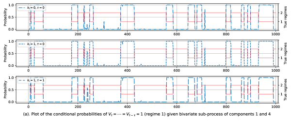
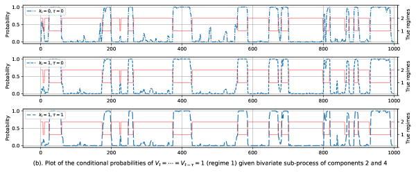
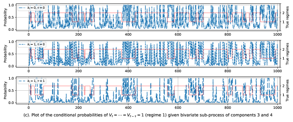
Fig. 1 (c) shows that for the sub-process composed of components 3 and 4, the latent regime switching cannot be correctly detected using the conditional probabilities. However, the results of latent regimes detection are better for the sub-process composed of components 2 and 4, and the latent regimes can be accurately inferred when it comes to the sub-process composed of components 1 and 4. It indicates that a model based on a sub-process whose univariate margins are similar across different regimes fails to detect the latent regime switching, even though there is a large difference in its cross-sectional correlations in different regimes. By comparing three subplots in Fig. 1 (a), one can see that fitting the serial correlation can slightly improve the results as the observations are simulated from a model of Markov order 1 within each regime. Moreover, the third subplot for $\tau=1$ shows a much smoother probability curve.

Refer to caption
Refer to caption
Figure 2: Plots (a) to (c): Scatterplots of observations and contour plots of fitted joint densities of different bivariate sub-processes. The fitted distributions are from the models fitting three subprocesses with Markov order $k_{i,g}=1$ for all $i=1,\dots,4$ and $g=1,2$. Plots (d) to (f): Univariate marginal histograms and fitted densities of components 1-3.

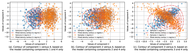
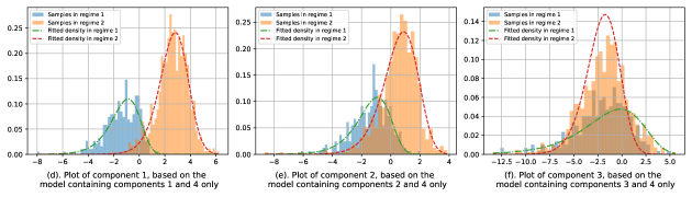
Using Fig. 2, a general conclusion can be drawn that the greater the distance between the univariate margins in different regimes, the better the inference for the latent regime sequence based on the sub-process involving these marginal components. The marginal density and contour plots in Fig. 2 can provide an intuitive explanation. Subplots (a) to (c) show the scatterplots and contours of the fitted densities for the considered three bivariate sub-processes, while subplots (d) to (f) display the univariate marginal histograms and fitted densities of univariate components 1 to 3. From subplots (a) and (d), one can observe that, for the bivariate sub-process composed of components 1 and 4, the observations in different regimes are well-separated. This is due to a large difference in the location parameters of the underlying distribution for marginal component 1 under the two regimes. As a result, the bivariate joint distributions of this sub-process can be accurately fitted in both regimes, even though there is no shift in margins under the two regimes for component 4. This also explains why the latent regime sequence can be correctly inferred using the sub-process with these two marginal components. For the bivariate sub-process composed of components 2 and 4, even though there is some distance between location parameters of the univariate margins of component 2 and the model can separate observations in the different regimes to some extent, the accuracy in inferring the latent regime sequence is diminished. Finally, for the last bivariate sub-process, plot (c) reveals that the model fails to identify the distributions in the two regimes even though their correlation parameters are quite different. This can be attributed to the lack of differences in the marginal distributions across the regimes as shown in plot (f). This failure of the model to discriminate between distributions for components 3 and 4 in the two regimes leads to the model’s inability to accurately infer the latent regime sequence when components 3 and 4 are used.

This study suggests that the subset selection of univariate components for the initial inference of the latent regime sequence should be based on those components whose univariate margins in different regimes can be well discriminated by a univariate hidden Markov model.

6 An empirical study on macroeconomic business cycle

This section contains the application of the margin-closed regime-switching model to the time series of macroeconomic indicators from the FRED-MD database (McCracken and Ng,, 2016). The database contains monthly series of many macroeconomic variables. Section 6.1 briefly introduces the data set. Section 6.2 fits the model with the given external business cycles information. Section 6.3 identifies the business cycle based only on the observed time series.

6.1 Macroeconomic indicators and business cycle

An available source of the business cycle information is the National Bureau of Economic Research (NBER, https://www.nber.org/research/data/us-business-cycle-expansions-and-contractions) of the United States. It is a nonprofit research organization serving a beneficial role in cataloging stylized facts about business cycles and providing a historical accounting of the dates of regime shifting for economic growth. For the macroeconomic indicators, the primary assumption that the series is stationary within each regime may be reasonable since all variables in the database have been transformed through differencing of natural log. To infer latent business cycle by fitting the margin-closed model, a subset of the indicators in the FRED database should be selected. Here, we choose the four key indicators mentioned by Chauvet and Papers, (2005): total personal income less transfer payments (income), the growth rates of manufacturing and trade sales (sales), civilian labor force employed in nonagricultural industries (employment), and industrial production (IP). All these variables are transformed to the first difference of natural log. The time series are available from June 1961 to February 2020, inclusive, for a total of 705 months.

6.2 Inference with external information

We first fit the proposed margin-closed regime-switching model to the selected four macroeconomic indicators and using the external business cycle information released by the NBER, with two regimes for economic recession and expansion.

As the univariate margins may have heavier tails and skewness compared with the Gaussian distribution, we fit them with the skew-t distribution (Jones and Faddy,, 2003) and transform to have the standard normal distribution.

For simplicity, the within-regime Markov orders for all univariate components are set to be equal, i.e., $k_{i,g}=k_{g}=k-1$ for all $i=1,\dots,4$ and $g=1,2$. In this case, one can take $k$ as $1$ plus the largest Markov order over all univariate time series. To determine the Markov order $k$ of the model, using the business cycle information from the NBER as a proxy for the latent regime sequence, we examined the plots of the sample autocorrelation function (ACF) and partial autocorrelation function (PACF). These plots (not shown in the paper) suggest that the largest Markov order across all univariate time series and all regimes is $4$. The AIC values of the models with different Markov orders are given in Table 4. Note that $k_{i,g}=0$ for $i=1,\dots,4$ and $g=1,2$ in the table indicates the hidden Markov model, where we also set $P=\bm{0}$. The results in Table 4 show that the models with $k_{i,g}=3,4,5$ have much smaller AIC values than those with $k_{i,g}=0,1,2$. This is consistent with the earlier assertion that $k_{i,g}=4$ based on the sample ACF and PACF plots. In the subsequent analysis, we set $k_{i,g}=3$ and $k=4$ for $i=1,\dots,4$ and $g=1,2$ as an optimal choice leading to the smallest AIC value.

Within-regime Markov order $k_{i,g}$ ($i=1,\dots,4,g=1,2$) 0 1 2 3 4 5
AIC 3884 3804 3789 3768 3771 3776
Table 4: The AIC values of models fitted with business cycle information given by NBER. The values are computed based on the complete likelihood of the known latent regime sequence and observations. Markov order of 0 leads to the hidden Markov model.

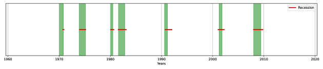
After determining the Markov order, we update the latent regime sequence (business cycle) following the approach in Section 4.1.2. It runs iteratively until the regime sequence stabilizes. For smoothing parameters in the latent regime sequence updating, we chose the same values as in Chauvet and Piger, (2008), i.e., $\tau=0$, $\nu=3$, and $\xi=0.8$. The results of the inferred business cycle are presented in Fig. 3. From the plot, we can see that the inferred business cycle updated based on the model has the same number of recession periods as that from the NBER. The differences include a delayed start and shorter duration of the first recession period, but longer recessions after the second recession period.

Refer to caption
Figure 3: Inferred business cycles from the model with $\tau=0$, $\nu=3$, and $\xi=0.8$, with the external business cycle information given by NBER. The red solid lines denote the inferred recession period, and the green shaded areas denote the NBER recession dates.

6.3 Inference based on the observed macroeconomic indicators only

We now fit the margin-closed regime-switching model and infer the business cycle based only on the observations of the four macroeconomic indicators.

We first fit the model using the multi-stage approach described in Section 4.2.1. In this case, both the Markov order $k$ and the number of different regimes $G$ should be determined for the model. Since the business cycle is usually modelled by two states of expansion and recession, we consider a model with three regimes for comparison. For all models, we let $g=1$ represent the recession and let higher values of $g$ indicate better economic situations. Therefore, models with two and three regimes and within-regime Markov orders from 00 to $5$ are considered. The AIC values for the fitted models are summarized in Table 5. Note that when $k_{i,g}=0$ for all $1\leq i\leq 4$ and $1\leq g\leq 3$, we also let $P=\bm{0}$ so that the model reduces to a hidden Markov model. According to the AIC values, models having the within-regime Markov order of $3$ are preferred in both cases of 2 and 3 regimes.

Within-regime Markov order $k_{i,g}$ ($i=1,\dots,4,g=1,2,3$) 0 1 2 3 4
AIC of models with two regimes 3897 3789 3768 3753 3759
AIC of models with three regimes 3812 3692 3679 3676 3689
Table 5: The AIC values of models fitted by multi-stage approach, without external business cycle information. Markov order of 0 in the table corresponds to the hidden Markov model.

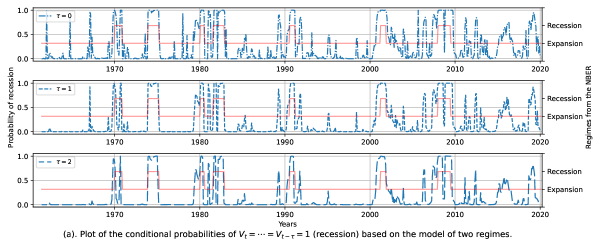
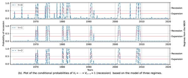
To further compare the two models with two and three regimes, Fig. 4 shows the estimates of the conditional probability of business recession given all observations, i.e., function $p_{t,\tau}(g)$ with $g=1$ and $\tau=0,1,2$ in the considered models. If we use the business cycles from the NBER as the benchmark, the plots show closer matches for the model with three regimes than the model with two regimes. Moreover, for both models, increasing the smoothing parameter $\tau$ from 00 to $1$ can improve the results as the fluctuations of the curves is reduced. But the benefit from further increasing $\tau$ to $2$ is minor as the curves corresponding to $\tau=1$ are already sufficiently smooth.

Refer to caption
Refer to caption
Figure 4: Inferred conditional probability of recession given all observations for the four indicators, based on models with two regimes (panel (a)) and three regimes (panel (b)).

We then apply the iterative procedure described in Section 4.2.2. Specifically, we employ the results of the hidden Markov model with independent univariate random variables in emission distributions as the starting point. Then, given the hyper-parameters $\tau,\nu,\xi$ in latent business cycle inference, the estimates of all model parameters and the inferred business cycles are updated iteratively until they stabilize. According to the outcomes shown in Fig. 4, $\tau=1$ is an appropriate choice for both models with two and three regimes.

Fig. 5 presents the results of the model with two regimes. One can see that the inferred business cycles are sensitive to the parameters $\nu$ and $\xi$. Compared with the business cycles given by the NBER, the large $\xi$ value of $0.8$ leads to a somewhat inadequate result as the fitted model fails to separate the third and fourth recession periods. Also, for $\nu=3$, the fitted model tends not to identify the first recession period. These results suggest that the value $\nu=2$ and a smaller $\xi$ value are preferable.

Refer to caption
Figure 5: Inferred latent regimes for parameter $\tau=1$ and different values $\nu,\xi$, based on the models with two regimes fitted using observations on four macroeconomic indicators. The red solid lines denote the inferred period of recession and the green shaded areas denote the NBER recession dates.

For the models with three regimes, we interpret the three states within a business cycle as recession, weak expansion, and strong expansion. Fig. 6 displays the inferred latent regimes from the model with three regimes for different values of $\nu$ and $\xi$. Note that the red solid lines denote the inferred periods of recession, the blue dot lines indicate periods of weak expansion, and blank periods are of strong expansion. Since there are three regimes in the model, we also try smaller values of $\xi$. Unlike the results of the model with two regimes, the inferred business cycles from the models with three regimes are more stable with respect to hyper-parameters $\nu$ and $\xi$. The main problem is that higher values of $\xi$ tend to lead to longer periods of the fifth recession and fail in separating the third and fourth recession periods. Moreover, the inferred starting time of the first recession period is still delayed compared with the period given by the NBER.

Refer to caption
Figure 6: Inferred latent regimes for parameter $\tau=1$ and different values of $\nu,\xi$, based on the models with three regimes (recession, weak expansion, strong expansion) fitted using only observations on four macroeconomic indicators. The red solid lines denote the inferred periods of recession, the blue dot lines denote the inferred periods of weak expansion, and the green shaded areas denote the NBER recession dates.

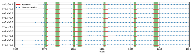
Based on Fig. 6, one can notice that the results for $\nu=2$ and $\xi=0.3$ can best match the business cycles from the NBER. To better explain this result, the mean and mode values of the four transformed macroeconomic indicators in different regimes are given in Table 6. It can be noticed that the means and modes of all indicators are negative in the recession, and they are all positive in the other two regimes, corresponding to $g=2$ and $g=3$. That is why $g=2$ and $g=3$ are interpreted as expansion, but the expansion indicated by $g=2$ is weaker than that of $g=3$. To compare the three regimes, Table 6 shows the cross-sectional correlation matrices of the four macroeconomic indicators in different regimes. They are the correlation matrices of the $4$-dimensional Gaussian copulas of the transformed indicators’ contemporaneous joint distributions in different regimes. It is seen that generally the four transformed indicators are more correlated in the recession and strong expansion periods than they are in weak expansion, except for the contemporaneous correlation between sales and employment, and the contemporaneous correlation between income and IP. It reflects that those macroeconomic indicators are more correlated in extreme economic situations. The interpretation of the inferred latent regimes is that even though the economy could be in expansion, most expansion periods after 1967 were of a weak expansion when those indicators had lower increment rates than the strong expansion before 1967.

Income Sales Employment IP
Mean Mode Mean Mode Mean Mode Mean Mode
Recession ($g=1$) -0.18 -0.11 -0.38 -0.56 -0.80 -0.54 -0.08 -0.05
Weak expansion ($g=2$) 0.29 0.29 0.23 0.19 0.21 0.23 0.14 0.15
Strong expansion ($g=3$) 0.38 0.47 0.71 1.04 0.76 0.74 0.22 0.22
Table 6: The mean and mode values of the four transformed macroeconomic indicators (%) in different regimes inferred using the model with three regimes.
Recession ($g=1$) Weak expansion ($g=2$) Strong expansion ($g=3$)
$R_{\bm{Y},g}$ $\left(\begin{smallmatrix}1&0.06&0.18&0.36\\ 0.06&1&0.51&0.18\\ 0.18&0.51&1&0.21\\ 0.36&0.18&0.21&1\end{smallmatrix}\right)$ $\left(\begin{smallmatrix}1&0.07&0.16&0.17\\ 0.07&1&0.40&0.08\\ 0.16&0.40&1&0.13\\ 0.17&0.08&0.13&1\end{smallmatrix}\right)$ $\left(\begin{smallmatrix}1&0.28&0.26&0.13\\ 0.28&1&0.18&0.26\\ 0.26&0.18&1&0.38\\ 0.13&0.26&0.38&1\end{smallmatrix}\right)$
Table 7: The contemporaneous cross-sectional correlations of the four macroeconomic indicators in different regimes inferred using the model with three regimes.

7 Discussion

The proposed margin-closed regime-switching multivariate time series model of Markov order $k$ implies that any subprocess of the multivariate time series is a regime-switching model with the same Markov order $k$ and the same latent regime sequence. It leads to a parsimonious regime-switching model and allows to make inference for the latent regime sequence based on a sub-process composed of some selected univariate components. Section 5 suggests selecting components that have the largest differences in univariate distributions under the different regimes. The proposed multivariate margin-closed regime-switching model is applied to a data set of four macroeconomic indicators, and the results show good performance on the inference for the latent business cycle.

One potential drawback of the proposed model is that the closure under margins property restricts the dependence between observations in different regimes. One way to deal with this is to introduce more parameters to capture serial dependence when transitioning between regimes. Alternatively, one can remove the restriction of closure under margins. This may be suitable when the dimension of the time series is low and the series is sufficiently long. A more general dependence between observations in different regimes can then be constructed through conditional independence, i.e., Condition 3 in Definition 3.1 can be replaced with the assumption that

$\displaystyle\mathchoice{\left[{{{{\bm{Y}_{t^{*}+\tilde{\ell}}\bot\bm{Y}_{t^{*}-\ell}}}}}\right]}{[{{{{\bm{Y}_{t^{*}+\tilde{\ell}}\bot\bm{Y}_{t^{*}-\ell}}}}}]}{[{{{{\bm{Y}_{t^{*}+\tilde{\ell}}\bot\bm{Y}_{t^{*}-\ell}}}}}]}{[{{{{\bm{Y}_{t^{*}+\tilde{\ell}}\bot\bm{Y}_{t^{*}-\ell}}}}}]}\big{|}\bm{Y}_{t^{*}+\tilde{\ell}-1},\dots,\bm{Y}_{t^{*}-\ell+1},\quad\forall\ \ell,\tilde{\ell}\geq 0\ \mbox{and}\ \tilde{\ell}+\ell>k,\ V_{t^{*}}\neq V_{t^{*}-1}.$ (44)

where $k$ is the Markov order of $\mathchoice{\left\{{{{{\bm{Y}_{t}}}}}\right\}}{\{{{{{\bm{Y}_{t}}}}}\}}{\{{{{{\bm{Y}_{t}}}}}\}}{\{{{{{\bm{Y}_{t}}}}}\}}_{t\in\mathbb{Z}}$, and only the correlation matrices $\operatorname{Cov}\mathchoice{\left({{{{\bm{Y}_{t^{*}+\tilde{\ell}},\bm{Y}_{t^{*}-\ell}}}}}\right)}{({{{{\bm{Y}_{t^{*}+\tilde{\ell}},\bm{Y}_{t^{*}-\ell}}}}})}{({{{{\bm{Y}_{t^{*}+\tilde{\ell}},\bm{Y}_{t^{*}-\ell}}}}})}{({{{{\bm{Y}_{t^{*}+\tilde{\ell}},\bm{Y}_{t^{*}-\ell}}}}})}$ for $\ell,\tilde{\ell}\geq 0$ and $\tilde{\ell}+\ell<=k$ need to be parameterized. In this case the dependence between observations in different regimes is fully modelled. Some advantages of this model formulation compared with other regime-switching models such as Markov switching vector autoregressive (MSVAR) models (see Cheng, (2016), Sola and Driffill, (1994), and Hamilton, (1990)) include the availability of thr stationary joint distributions of observations within each regime and the possibility to be extended to models with non-Gaussian margins.

Appendix A Parameterization of margin-closed VAR model

Let $\bm{C}_{i}=\mathchoice{\left({{{{Z_{i,t},\dots,Z_{i,t-k}}}}}\right)}{({{{{Z_{i,t},\dots,Z_{i,t-k}}}}})}{({{{{Z_{i,t},\dots,Z_{i,t-k}}}}})}{({{{{Z_{i,t},\dots,Z_{i,t-k}}}}})}^{\top}$. To get $R_{\bm{Z}_{t:(t-k)}}$ from $R_{Z_{i,t:(t-k)}}$ for $1\leq i\leq d$ and $R_{\bm{Z}}$, one can firstly derive

$\displaystyle R_{\mathchoice{\left\{{{{{1,\dots,d}}}}\right\}}{\{{{{{1,\dots,d}}}}\}}{\{{{{{1,\dots,d}}}}\}}{\{{{{{1,\dots,d}}}}\}}}=\operatorname{Corr}\mathchoice{\left({{{{\mathchoice{\left({{{{Z_{1,t},\dots,Z_{d,t},\dots,Z_{1,t-k},\dots,Z_{d,t-k}}}}}\right)}{({{{{Z_{1,t},\dots,Z_{d,t},\dots,Z_{1,t-k},\dots,Z_{d,t-k}}}}})}{({{{{Z_{1,t},\dots,Z_{d,t},\dots,Z_{1,t-k},\dots,Z_{d,t-k}}}}})}{({{{{Z_{1,t},\dots,Z_{d,t},\dots,Z_{1,t-k},\dots,Z_{d,t-k}}}}})}}}}}\right)}{({{{{\mathchoice{\left({{{{Z_{1,t},\dots,Z_{d,t},\dots,Z_{1,t-k},\dots,Z_{d,t-k}}}}}\right)}{({{{{Z_{1,t},\dots,Z_{d,t},\dots,Z_{1,t-k},\dots,Z_{d,t-k}}}}})}{({{{{Z_{1,t},\dots,Z_{d,t},\dots,Z_{1,t-k},\dots,Z_{d,t-k}}}}})}{({{{{Z_{1,t},\dots,Z_{d,t},\dots,Z_{1,t-k},\dots,Z_{d,t-k}}}}})}}}}})}{({{{{\mathchoice{\left({{{{Z_{1,t},\dots,Z_{d,t},\dots,Z_{1,t-k},\dots,Z_{d,t-k}}}}}\right)}{({{{{Z_{1,t},\dots,Z_{d,t},\dots,Z_{1,t-k},\dots,Z_{d,t-k}}}}})}{({{{{Z_{1,t},\dots,Z_{d,t},\dots,Z_{1,t-k},\dots,Z_{d,t-k}}}}})}{({{{{Z_{1,t},\dots,Z_{d,t},\dots,Z_{1,t-k},\dots,Z_{d,t-k}}}}})}}}}})}{({{{{\mathchoice{\left({{{{Z_{1,t},\dots,Z_{d,t},\dots,Z_{1,t-k},\dots,Z_{d,t-k}}}}}\right)}{({{{{Z_{1,t},\dots,Z_{d,t},\dots,Z_{1,t-k},\dots,Z_{d,t-k}}}}})}{({{{{Z_{1,t},\dots,Z_{d,t},\dots,Z_{1,t-k},\dots,Z_{d,t-k}}}}})}{({{{{Z_{1,t},\dots,Z_{d,t},\dots,Z_{1,t-k},\dots,Z_{d,t-k}}}}})}}}}})}=\operatorname{Corr}\mathchoice{\left({{{{\mathchoice{\left({{{{\bm{C}_{1}^{\top},\dots,\bm{C}_{d}^{\top}}}}}\right)}{({{{{\bm{C}_{1}^{\top},\dots,\bm{C}_{d}^{\top}}}}})}{({{{{\bm{C}_{1}^{\top},\dots,\bm{C}_{d}^{\top}}}}})}{({{{{\bm{C}_{1}^{\top},\dots,\bm{C}_{d}^{\top}}}}})}^{\top}}}}}\right)}{({{{{\mathchoice{\left({{{{\bm{C}_{1}^{\top},\dots,\bm{C}_{d}^{\top}}}}}\right)}{({{{{\bm{C}_{1}^{\top},\dots,\bm{C}_{d}^{\top}}}}})}{({{{{\bm{C}_{1}^{\top},\dots,\bm{C}_{d}^{\top}}}}})}{({{{{\bm{C}_{1}^{\top},\dots,\bm{C}_{d}^{\top}}}}})}^{\top}}}}})}{({{{{\mathchoice{\left({{{{\bm{C}_{1}^{\top},\dots,\bm{C}_{d}^{\top}}}}}\right)}{({{{{\bm{C}_{1}^{\top},\dots,\bm{C}_{d}^{\top}}}}})}{({{{{\bm{C}_{1}^{\top},\dots,\bm{C}_{d}^{\top}}}}})}{({{{{\bm{C}_{1}^{\top},\dots,\bm{C}_{d}^{\top}}}}})}^{\top}}}}})}{({{{{\mathchoice{\left({{{{\bm{C}_{1}^{\top},\dots,\bm{C}_{d}^{\top}}}}}\right)}{({{{{\bm{C}_{1}^{\top},\dots,\bm{C}_{d}^{\top}}}}})}{({{{{\bm{C}_{1}^{\top},\dots,\bm{C}_{d}^{\top}}}}})}{({{{{\bm{C}_{1}^{\top},\dots,\bm{C}_{d}^{\top}}}}})}^{\top}}}}})}.$ (45)

Then $R_{\bm{Z}_{t:(t-k)}}$ can be obtained by reordering rows and columns of $R_{\mathchoice{\left\{{{{{1,\dots,d}}}}\right\}}{\{{{{{1,\dots,d}}}}\}}{\{{{{{1,\dots,d}}}}\}}{\{{{{{1,\dots,d}}}}\}}}$. The definitions of $R_{\mathchoice{\left\{{{{{1,\dots,d}}}}\right\}}{\{{{{{1,\dots,d}}}}\}}{\{{{{{1,\dots,d}}}}\}}{\{{{{{1,\dots,d}}}}\}}}$ and $R_{Z_{i,t:(t-k)}}$ for $1\leq i\leq d$ lead to

R{1,,d}=(RZ1,t:(tk)Corr(𝑪1,𝑪2)Corr(𝑪1,𝑪d)Corr(𝑪1,𝑪2)TRZ2,t:(tk)Corr(𝑪2,𝑪d1)Corr(𝑪1,𝑪d)TCorr(𝑪2,𝑪d1)TRZd,t:(tk)),\addcontentsline{lla}{section}{\numberline{\string\crtrefnumber{eq:correlation_matrix_of_Z1_to_Zn}}{e}q:correlation_{m}atrix_{o}f_{Z}1_{t}o_{Z}n}R_{\mathchoice{\left\{{{{{1,\dots,d}}}}\right\}}{\{{{{{1,\dots,d}}}}\}}{\{{{{{1,\dots,d}}}}\}}{\{{{{{1,\dots,d}}}}\}}}=\begin{pmatrix}R_{Z_{1,t:(t-k)}}&\operatorname{Corr}\mathchoice{\left({{{{\bm{C}_{1},\bm{C}_{2}}}}}\right)}{({{{{\bm{C}_{1},\bm{C}_{2}}}}})}{({{{{\bm{C}_{1},\bm{C}_{2}}}}})}{({{{{\bm{C}_{1},\bm{C}_{2}}}}})}&\cdots&\operatorname{Corr}\mathchoice{\left({{{{\bm{C}_{1},\bm{C}_{d}}}}}\right)}{({{{{\bm{C}_{1},\bm{C}_{d}}}}})}{({{{{\bm{C}_{1},\bm{C}_{d}}}}})}{({{{{\bm{C}_{1},\bm{C}_{d}}}}})}\\ \operatorname{Corr}\mathchoice{\left({{{{\bm{C}_{1},\bm{C}_{2}}}}}\right)}{({{{{\bm{C}_{1},\bm{C}_{2}}}}})}{({{{{\bm{C}_{1},\bm{C}_{2}}}}})}{({{{{\bm{C}_{1},\bm{C}_{2}}}}})}^{T}&R_{Z_{2,t:(t-k)}}&\cdots&\operatorname{Corr}\mathchoice{\left({{{{\bm{C}_{2},\bm{C}_{d-1}}}}}\right)}{({{{{\bm{C}_{2},\bm{C}_{d-1}}}}})}{({{{{\bm{C}_{2},\bm{C}_{d-1}}}}})}{({{{{\bm{C}_{2},\bm{C}_{d-1}}}}})}\\ \vdots&\vdots&\ddots&\vdots\\ \operatorname{Corr}\mathchoice{\left({{{{\bm{C}_{1},\bm{C}_{d}}}}}\right)}{({{{{\bm{C}_{1},\bm{C}_{d}}}}})}{({{{{\bm{C}_{1},\bm{C}_{d}}}}})}{({{{{\bm{C}_{1},\bm{C}_{d}}}}})}^{T}&\operatorname{Corr}\mathchoice{\left({{{{\bm{C}_{2},\bm{C}_{d-1}}}}}\right)}{({{{{\bm{C}_{2},\bm{C}_{d-1}}}}})}{({{{{\bm{C}_{2},\bm{C}_{d-1}}}}})}{({{{{\bm{C}_{2},\bm{C}_{d-1}}}}})}^{T}&\cdots&R_{Z_{d,t:(t-k)}}\end{pmatrix}, (46)

where $\operatorname{Corr}\mathchoice{\left({{{{\bm{C}_{i},\bm{C}_{j}}}}}\right)}{({{{{\bm{C}_{i},\bm{C}_{j}}}}})}{({{{{\bm{C}_{i},\bm{C}_{j}}}}})}{({{{{\bm{C}_{i},\bm{C}_{j}}}}})}$ for $1\leq i<j\leq d$ can be derived by the formulas given below.

For $1\leq p\leq d$, let

$\displaystyle R_{Z_{p,t:(t-k)}}=\begin{pmatrix}1&\varrho_{p,1}&\cdots&\varrho_{p,k}\\ \varrho_{p,1}&1&\cdots&\varrho_{p,k-1}\\ \vdots&\vdots&\ddots&\vdots\\ \varrho_{p,k}&\varrho_{p,k-1}&\cdots&1\end{pmatrix}$ (47)

and

$$H_{p}=\begin{pmatrix}-I_{d_{p}}&\psi_{p,k}&\dots&\psi_{p,2}&\psi_{p,1}&0&0&\cdots&0\\ 0&-I_{d_{p}}&\psi_{p,k}&\dots&\psi_{p,2}&\psi_{p,1}&0&\cdots&0\\ \vdots&\ddots&\ddots&\ddots&\ddots&\ddots&\ddots&\ddots&\vdots\\ 0&\cdots&0&-I_{d_{p}}&\psi_{p,k}&\cdots&\psi_{p,2}&\psi_{p,1}&0\end{pmatrix},$$ (48)

where

$$\begin{pmatrix}\psi_{p,1}&\psi_{p,2}&\cdots&\psi_{p,k}\\ \end{pmatrix}^{\top}=\begin{pmatrix}\varrho_{p,-k}&\varrho_{p,1-k}&\cdots&\varrho_{p,-1}\\ \end{pmatrix}^{\top}\begin{pmatrix}1&\varrho_{p,1}&\cdots&\varrho_{p,k-1}\\ \varrho_{p,1}&1&\cdots&\varrho_{p,k-2}\\ \vdots&\vdots&\ddots&\vdots\\ \varrho_{p,k-1}&\varrho_{p,k-2}&\cdots&1\end{pmatrix}^{-1},$$ (49)

and $\varrho_{p,-m}=\varrho_{p,m}$. Let $H_{p:(k+1)}$ denote the submatrix of the $(k+1)$-th block column of $H_{p}$ and $H_{p,:-(k+1)}$ denote the submatrix obtained by removing the $(k+1)$-th block column of $H_{p}$. If $A=(a_{ij})$ is an $m\times n$ matrix, the Kronecker product $A\otimes B$ is defined as

$\displaystyle\begin{pmatrix}a_{11}B&\cdots&a_{1n}B\\ \vdots&\ddots&\vdots\\ a_{m1}B&\cdots&a_{mn}B\\ \end{pmatrix}.$ (50)

Let $L$ be the $(2k+1)$-dimensional exchange (or permutation) matrix whose elements in the anti-diagonal are one and all other elements are zero. Let $\varrho_{ij,0}=\operatorname{Corr}\mathchoice{\left({{{{Z_{i,t},Z_{j,t}}}}}\right)}{({{{{Z_{i,t},Z_{j,t}}}}})}{({{{{Z_{i,t},Z_{j,t}}}}})}{({{{{Z_{i,t},Z_{j,t}}}}})}$ for $i\neq j$; this is an element of $R_{\bm{Z}}$. Then

$\displaystyle\operatorname{Corr}\mathchoice{\left({{{{\bm{C}_{i},\bm{C}_{j}}}}}\right)}{({{{{\bm{C}_{i},\bm{C}_{j}}}}})}{({{{{\bm{C}_{i},\bm{C}_{j}}}}})}{({{{{\bm{C}_{i},\bm{C}_{j}}}}})}=\begin{pmatrix}\varrho_{ij,0}&\varrho_{ij,1}&\cdots&\varrho_{ij,k-1}\\ \varrho_{ij,-1}&\varrho_{ij,0}&\cdots&\varrho_{ij,k-2}\\ \vdots&\vdots&\ddots&\vdots\\ \varrho_{ij,1-k}&\varrho_{ij,2-k}&\cdots&\varrho_{ij,0}\end{pmatrix},$ (51)

where

$$\mathchoice{\left({{{{\varrho_{ij,-k},\dots,\varrho_{ij,-1},\varrho_{ij,1},\dots,\varrho_{ij,k}}}}}\right)}{({{{{\varrho_{ij,-k},\dots,\varrho_{ij,-1},\varrho_{ij,1},\dots,\varrho_{ij,k}}}}})}{({{{{\varrho_{ij,-k},\dots,\varrho_{ij,-1},\varrho_{ij,1},\dots,\varrho_{ij,k}}}}})}{({{{{\varrho_{ij,-k},\dots,\varrho_{ij,-1},\varrho_{ij,1},\dots,\varrho_{ij,k}}}}})}^{\top}=-\varrho_{ij,0}\begin{pmatrix}H_{i,:-(k+1)}\\ \mathchoice{\left({{{{H_{j}L}}}}\right)}{({{{{H_{j}L}}}})}{({{{{H_{j}L}}}})}{({{{{H_{j}L}}}})}_{:-(k+1)}\end{pmatrix}^{-1}\begin{pmatrix}H_{i,:(k+1)}\\ H_{j,:(k+1)}\end{pmatrix}.$$ (52)

Appendix B Proof of Proposition 3.2

Part 1 (The process is Markov of order $k$)

Suppose the process changes from regime $g_{b}$ at time $t^{*}-1$ to regime $g^{\prime}$ at time $t^{*}$. Because $\{\bm{Y}_{t}\}$ is a Gaussian process, $\bm{Y}_{t^{*}}$ is independent of $\bm{Y}_{t^{*}-\ell-1}$ given $\bm{Y}_{t^{*}-1}$ for any $\ell$ with $\ell\geq 1$, implying

[𝒀t|𝒀t1,,𝒀1]=d[𝒀t|𝒀t1].delimited-[]conditionalsubscript𝒀superscript𝑡subscript𝒀superscript𝑡1subscript𝒀1ddelimited-[]conditionalsubscript𝒀superscript𝑡subscript𝒀superscript𝑡1\addcontentsline{lla}{section}{\numberline{\string\crtrefnumber{eq:con_dist1}}{e}q:con_{d}ist1}\mathchoice{\left[{{{{\bm{Y}_{t^{*}}\big{|}\bm{Y}_{t^{*}-1},\dots,\bm{Y}_{1}}}}}\right]}{[{{{{\bm{Y}_{t^{*}}\big{|}\bm{Y}_{t^{*}-1},\dots,\bm{Y}_{1}}}}}]}{[{{{{\bm{Y}_{t^{*}}\big{|}\bm{Y}_{t^{*}-1},\dots,\bm{Y}_{1}}}}}]}{[{{{{\bm{Y}_{t^{*}}\big{|}\bm{Y}_{t^{*}-1},\dots,\bm{Y}_{1}}}}}]}\overset{\mathrm{d}}{=}\mathchoice{\left[{{{{\bm{Y}_{t^{*}}\big{|}\bm{Y}_{t^{*}-1}}}}}\right]}{[{{{{\bm{Y}_{t^{*}}\big{|}\bm{Y}_{t^{*}-1}}}}}]}{[{{{{\bm{Y}_{t^{*}}\big{|}\bm{Y}_{t^{*}-1}}}}}]}{[{{{{\bm{Y}_{t^{*}}\big{|}\bm{Y}_{t^{*}-1}}}}}]}. (53)

From the covariance matrix of conditional distributions of multivariate Gaussian random vectors, Eq. 7 implies

Cov(𝒀t+~,𝒀t1|𝒀t1)=Cov(𝒀t+~,𝒀t1)Cov(𝒀t+~,𝒀t1)[Cov(𝒀t1,𝒀t1)]1Cov(𝒀t1,𝒀t1)=𝟎,Covsubscript𝒀superscript𝑡~conditionalsubscript𝒀superscript𝑡1subscript𝒀superscript𝑡1Covsubscript𝒀superscript𝑡~subscript𝒀superscript𝑡1Covsubscript𝒀superscript𝑡~subscript𝒀superscript𝑡1superscriptdelimited-[]Covsubscript𝒀superscript𝑡1subscript𝒀superscript𝑡11Covsubscript𝒀superscript𝑡1subscript𝒀superscript𝑡10\addcontentsline{lla}{section}{\numberline{\string\crtrefnumber{eq:condition3.1}}{e}q:condition3.1}\begin{split}&\operatorname{Cov}\mathchoice{\left({{{{\bm{Y}_{t^{*}+\tilde{\ell}},\bm{Y}_{t^{*}-\ell-1}\big{|}\bm{Y}_{t^{*}-1}}}}}\right)}{({{{{\bm{Y}_{t^{*}+\tilde{\ell}},\bm{Y}_{t^{*}-\ell-1}\big{|}\bm{Y}_{t^{*}-1}}}}})}{({{{{\bm{Y}_{t^{*}+\tilde{\ell}},\bm{Y}_{t^{*}-\ell-1}\big{|}\bm{Y}_{t^{*}-1}}}}})}{({{{{\bm{Y}_{t^{*}+\tilde{\ell}},\bm{Y}_{t^{*}-\ell-1}\big{|}\bm{Y}_{t^{*}-1}}}}})}=\operatorname{Cov}\mathchoice{\left({{{{\bm{Y}_{t^{*}+\tilde{\ell}},\bm{Y}_{t^{*}-\ell-1}}}}}\right)}{({{{{\bm{Y}_{t^{*}+\tilde{\ell}},\bm{Y}_{t^{*}-\ell-1}}}}})}{({{{{\bm{Y}_{t^{*}+\tilde{\ell}},\bm{Y}_{t^{*}-\ell-1}}}}})}{({{{{\bm{Y}_{t^{*}+\tilde{\ell}},\bm{Y}_{t^{*}-\ell-1}}}}})}\\ &\hskip 28.45274pt-\operatorname{Cov}\mathchoice{\left({{{{\bm{Y}_{t^{*}+\tilde{\ell}},\bm{Y}_{t^{*}-1}}}}}\right)}{({{{{\bm{Y}_{t^{*}+\tilde{\ell}},\bm{Y}_{t^{*}-1}}}}})}{({{{{\bm{Y}_{t^{*}+\tilde{\ell}},\bm{Y}_{t^{*}-1}}}}})}{({{{{\bm{Y}_{t^{*}+\tilde{\ell}},\bm{Y}_{t^{*}-1}}}}})}[\operatorname{Cov}\mathchoice{\left({{{{\bm{Y}_{t^{*}-1},\bm{Y}_{t^{*}-1}}}}}\right)}{({{{{\bm{Y}_{t^{*}-1},\bm{Y}_{t^{*}-1}}}}})}{({{{{\bm{Y}_{t^{*}-1},\bm{Y}_{t^{*}-1}}}}})}{({{{{\bm{Y}_{t^{*}-1},\bm{Y}_{t^{*}-1}}}}})}]^{-1}\operatorname{Cov}\mathchoice{\left({{{{\bm{Y}_{t^{*}-1},\bm{Y}_{t^{*}-\ell-1}}}}}\right)}{({{{{\bm{Y}_{t^{*}-1},\bm{Y}_{t^{*}-\ell-1}}}}})}{({{{{\bm{Y}_{t^{*}-1},\bm{Y}_{t^{*}-\ell-1}}}}})}{({{{{\bm{Y}_{t^{*}-1},\bm{Y}_{t^{*}-\ell-1}}}}})}=\bm{0},\end{split}

for any $\ell,\tilde{\ell}\geq 1$. Combining Eq. 6 and Appendix B, by induction,

$\displaystyle\mathchoice{\left[{{{{\bm{Y}_{t^{*}+\tilde{\ell}}\bot\bm{Y}_{t^{*}-\ell-1}}}}}\right]}{[{{{{\bm{Y}_{t^{*}+\tilde{\ell}}\bot\bm{Y}_{t^{*}-\ell-1}}}}}]}{[{{{{\bm{Y}_{t^{*}+\tilde{\ell}}\bot\bm{Y}_{t^{*}-\ell-1}}}}}]}{[{{{{\bm{Y}_{t^{*}+\tilde{\ell}}\bot\bm{Y}_{t^{*}-\ell-1}}}}}]}\big{|}\bm{Y}_{t^{*}+\tilde{\ell}-1},\dots,\bm{Y}_{t^{*}-1},$ (54)

i.e.,

[𝒀t+~|𝒀t+~1,,𝒀1]=d[𝒀t+~|𝒀t+~1,,𝒀t1].delimited-[]conditionalsubscript𝒀superscript𝑡~subscript𝒀superscript𝑡~1subscript𝒀1ddelimited-[]conditionalsubscript𝒀superscript𝑡~subscript𝒀superscript𝑡~1subscript𝒀superscript𝑡1\addcontentsline{lla}{section}{\numberline{\string\crtrefnumber{eq:con_dist2}}{e}q:con_{d}ist2}\mathchoice{\left[{{{{\bm{Y}_{t^{*}+\tilde{\ell}}\big{|}\bm{Y}_{t^{*}+\tilde{\ell}-1},\dots,\bm{Y}_{1}}}}}\right]}{[{{{{\bm{Y}_{t^{*}+\tilde{\ell}}\big{|}\bm{Y}_{t^{*}+\tilde{\ell}-1},\dots,\bm{Y}_{1}}}}}]}{[{{{{\bm{Y}_{t^{*}+\tilde{\ell}}\big{|}\bm{Y}_{t^{*}+\tilde{\ell}-1},\dots,\bm{Y}_{1}}}}}]}{[{{{{\bm{Y}_{t^{*}+\tilde{\ell}}\big{|}\bm{Y}_{t^{*}+\tilde{\ell}-1},\dots,\bm{Y}_{1}}}}}]}\overset{\mathrm{d}}{=}\mathchoice{\left[{{{{\bm{Y}_{t^{*}+\tilde{\ell}}\big{|}\bm{Y}_{t^{*}+\tilde{\ell}-1},\dots,\bm{Y}_{t^{*}-1}}}}}\right]}{[{{{{\bm{Y}_{t^{*}+\tilde{\ell}}\big{|}\bm{Y}_{t^{*}+\tilde{\ell}-1},\dots,\bm{Y}_{t^{*}-1}}}}}]}{[{{{{\bm{Y}_{t^{*}+\tilde{\ell}}\big{|}\bm{Y}_{t^{*}+\tilde{\ell}-1},\dots,\bm{Y}_{t^{*}-1}}}}}]}{[{{{{\bm{Y}_{t^{*}+\tilde{\ell}}\big{|}\bm{Y}_{t^{*}+\tilde{\ell}-1},\dots,\bm{Y}_{t^{*}-1}}}}}]}. (55)

To prove that process $\{\bm{Y}_{t}\}$ is Markov of order $k$ need to show that the right hand side of Eq. 55 can be reduced to at most $k$ conditioning variables. Hence, only the situation when $\tilde{\ell}>k$ and $v_{t^{*}}=v_{t^{*}+1}=\cdots=v_{t^{*}+\tilde{\ell}}=g^{\prime}$ needs to be considered. Let

$\displaystyle\bm{A}_{t^{*}+\tilde{\ell}}$ $\displaystyle=\mathchoice{\left({{{{\bm{Y}^{\top}_{t^{*}+\tilde{\ell}-1},\dots,\bm{Y}^{\top}_{t^{*}+\tilde{\ell}-k+1}}}}}\right)}{({{{{\bm{Y}^{\top}_{t^{*}+\tilde{\ell}-1},\dots,\bm{Y}^{\top}_{t^{*}+\tilde{\ell}-k+1}}}}})}{({{{{\bm{Y}^{\top}_{t^{*}+\tilde{\ell}-1},\dots,\bm{Y}^{\top}_{t^{*}+\tilde{\ell}-k+1}}}}})}{({{{{\bm{Y}^{\top}_{t^{*}+\tilde{\ell}-1},\dots,\bm{Y}^{\top}_{t^{*}+\tilde{\ell}-k+1}}}}})}^{\top}.$ (56)

Since the process is Markov of order $k-1=\max_{1\leq g\leq G}k_{g}$ within any regime,

$\displaystyle\mathchoice{\left[{{{{\bm{Y}_{t^{*}+\tilde{\ell}}\bot\mathchoice{\left({{{{\bm{Y}^{\top}_{t^{*}+\tilde{\ell}-k},\dots,\bm{Y}^{\top}_{t^{*}}}}}}\right)}{({{{{\bm{Y}^{\top}_{t^{*}+\tilde{\ell}-k},\dots,\bm{Y}^{\top}_{t^{*}}}}}})}{({{{{\bm{Y}^{\top}_{t^{*}+\tilde{\ell}-k},\dots,\bm{Y}^{\top}_{t^{*}}}}}})}{({{{{\bm{Y}^{\top}_{t^{*}+\tilde{\ell}-k},\dots,\bm{Y}^{\top}_{t^{*}}}}}})}^{\top}}}}}\right]}{[{{{{\bm{Y}_{t^{*}+\tilde{\ell}}\bot\mathchoice{\left({{{{\bm{Y}^{\top}_{t^{*}+\tilde{\ell}-k},\dots,\bm{Y}^{\top}_{t^{*}}}}}}\right)}{({{{{\bm{Y}^{\top}_{t^{*}+\tilde{\ell}-k},\dots,\bm{Y}^{\top}_{t^{*}}}}}})}{({{{{\bm{Y}^{\top}_{t^{*}+\tilde{\ell}-k},\dots,\bm{Y}^{\top}_{t^{*}}}}}})}{({{{{\bm{Y}^{\top}_{t^{*}+\tilde{\ell}-k},\dots,\bm{Y}^{\top}_{t^{*}}}}}})}^{\top}}}}}]}{[{{{{\bm{Y}_{t^{*}+\tilde{\ell}}\bot\mathchoice{\left({{{{\bm{Y}^{\top}_{t^{*}+\tilde{\ell}-k},\dots,\bm{Y}^{\top}_{t^{*}}}}}}\right)}{({{{{\bm{Y}^{\top}_{t^{*}+\tilde{\ell}-k},\dots,\bm{Y}^{\top}_{t^{*}}}}}})}{({{{{\bm{Y}^{\top}_{t^{*}+\tilde{\ell}-k},\dots,\bm{Y}^{\top}_{t^{*}}}}}})}{({{{{\bm{Y}^{\top}_{t^{*}+\tilde{\ell}-k},\dots,\bm{Y}^{\top}_{t^{*}}}}}})}^{\top}}}}}]}{[{{{{\bm{Y}_{t^{*}+\tilde{\ell}}\bot\mathchoice{\left({{{{\bm{Y}^{\top}_{t^{*}+\tilde{\ell}-k},\dots,\bm{Y}^{\top}_{t^{*}}}}}}\right)}{({{{{\bm{Y}^{\top}_{t^{*}+\tilde{\ell}-k},\dots,\bm{Y}^{\top}_{t^{*}}}}}})}{({{{{\bm{Y}^{\top}_{t^{*}+\tilde{\ell}-k},\dots,\bm{Y}^{\top}_{t^{*}}}}}})}{({{{{\bm{Y}^{\top}_{t^{*}+\tilde{\ell}-k},\dots,\bm{Y}^{\top}_{t^{*}}}}}})}^{\top}}}}}]}\Bigm{|}\bm{A}_{t^{*}+\tilde{\ell}}.$ (57)

Moreover, the condition in Eq. 7 implies $\bm{A}_{t^{*}+\tilde{\ell}}\bot\bm{Y}_{t^{*}-1}$, and leads to

$\displaystyle\operatorname{Cov}\mathchoice{\left({{{{\bm{Y}_{t^{*}+\tilde{\ell}},\bm{Y}_{t^{*}-1}\big{|}\bm{A}_{t^{*}+\tilde{\ell}}}}}}\right)}{({{{{\bm{Y}_{t^{*}+\tilde{\ell}},\bm{Y}_{t^{*}-1}\big{|}\bm{A}_{t^{*}+\tilde{\ell}}}}}})}{({{{{\bm{Y}_{t^{*}+\tilde{\ell}},\bm{Y}_{t^{*}-1}\big{|}\bm{A}_{t^{*}+\tilde{\ell}}}}}})}{({{{{\bm{Y}_{t^{*}+\tilde{\ell}},\bm{Y}_{t^{*}-1}\big{|}\bm{A}_{t^{*}+\tilde{\ell}}}}}})}$ (58)
$\displaystyle=$ $\displaystyle\operatorname{Cov}\mathchoice{\left({{{{\bm{Y}_{t^{*}+\tilde{\ell}},\bm{Y}_{t^{*}-1}}}}}\right)}{({{{{\bm{Y}_{t^{*}+\tilde{\ell}},\bm{Y}_{t^{*}-1}}}}})}{({{{{\bm{Y}_{t^{*}+\tilde{\ell}},\bm{Y}_{t^{*}-1}}}}})}{({{{{\bm{Y}_{t^{*}+\tilde{\ell}},\bm{Y}_{t^{*}-1}}}}})}-\operatorname{Cov}\mathchoice{\left({{{{\bm{Y}_{t^{*}+\tilde{\ell}},\bm{A}_{t^{*}+\tilde{\ell}}}}}}\right)}{({{{{\bm{Y}_{t^{*}+\tilde{\ell}},\bm{A}_{t^{*}+\tilde{\ell}}}}}})}{({{{{\bm{Y}_{t^{*}+\tilde{\ell}},\bm{A}_{t^{*}+\tilde{\ell}}}}}})}{({{{{\bm{Y}_{t^{*}+\tilde{\ell}},\bm{A}_{t^{*}+\tilde{\ell}}}}}})}[\operatorname{Cov}\mathchoice{\left({{{{\bm{A}_{t^{*}+\tilde{\ell}},\bm{A}_{t^{*}+\tilde{\ell}}}}}}\right)}{({{{{\bm{A}_{t^{*}+\tilde{\ell}},\bm{A}_{t^{*}+\tilde{\ell}}}}}})}{({{{{\bm{A}_{t^{*}+\tilde{\ell}},\bm{A}_{t^{*}+\tilde{\ell}}}}}})}{({{{{\bm{A}_{t^{*}+\tilde{\ell}},\bm{A}_{t^{*}+\tilde{\ell}}}}}})}]^{-1}\operatorname{Cov}\mathchoice{\left({{{{\bm{A}_{t^{*}+\tilde{\ell}},\bm{Y}_{t^{*}-1}}}}}\right)}{({{{{\bm{A}_{t^{*}+\tilde{\ell}},\bm{Y}_{t^{*}-1}}}}})}{({{{{\bm{A}_{t^{*}+\tilde{\ell}},\bm{Y}_{t^{*}-1}}}}})}{({{{{\bm{A}_{t^{*}+\tilde{\ell}},\bm{Y}_{t^{*}-1}}}}})}$ (59)
$\displaystyle=$ $\displaystyle\bm{0}-\operatorname{Cov}\mathchoice{\left({{{{\bm{Y}_{t^{*}+\tilde{\ell}},\bm{A}_{t^{*}+\tilde{\ell}}}}}}\right)}{({{{{\bm{Y}_{t^{*}+\tilde{\ell}},\bm{A}_{t^{*}+\tilde{\ell}}}}}})}{({{{{\bm{Y}_{t^{*}+\tilde{\ell}},\bm{A}_{t^{*}+\tilde{\ell}}}}}})}{({{{{\bm{Y}_{t^{*}+\tilde{\ell}},\bm{A}_{t^{*}+\tilde{\ell}}}}}})}\operatorname{Cov}^{-1}\mathchoice{\left({{{{\bm{A}_{t^{*}+\tilde{\ell}},\bm{A}_{t^{*}+\tilde{\ell}}}}}}\right)}{({{{{\bm{A}_{t^{*}+\tilde{\ell}},\bm{A}_{t^{*}+\tilde{\ell}}}}}})}{({{{{\bm{A}_{t^{*}+\tilde{\ell}},\bm{A}_{t^{*}+\tilde{\ell}}}}}})}{({{{{\bm{A}_{t^{*}+\tilde{\ell}},\bm{A}_{t^{*}+\tilde{\ell}}}}}})}\bm{0}=\bm{0}.$ (60)

According to Eq. 55, it implies that if $\tilde{\ell}>k$, then

$$\ignorespaces\ignorespaces\mathchoice{\left[{{{{\bm{Y}_{t^{*}+\tilde{\ell}}\big{|}\bm{Y}_{t^{*}+\tilde{\ell}-1},\dots,\bm{Y}_{1}}}}}\right]}{[{{{{\bm{Y}_{t^{*}+\tilde{\ell}}\big{|}\bm{Y}_{t^{*}+\tilde{\ell}-1},\dots,\bm{Y}_{1}}}}}]}{[{{{{\bm{Y}_{t^{*}+\tilde{\ell}}\big{|}\bm{Y}_{t^{*}+\tilde{\ell}-1},\dots,\bm{Y}_{1}}}}}]}{[{{{{\bm{Y}_{t^{*}+\tilde{\ell}}\big{|}\bm{Y}_{t^{*}+\tilde{\ell}-1},\dots,\bm{Y}_{1}}}}}]}\overset{\mathrm{d}}{=}\mathchoice{\left[{{{{\bm{Y}_{t^{*}+\tilde{\ell}}\big{|}\bm{Y}_{t^{*}+\tilde{\ell}-1},\dots,\bm{Y}_{t^{*}-1}}}}}\right]}{[{{{{\bm{Y}_{t^{*}+\tilde{\ell}}\big{|}\bm{Y}_{t^{*}+\tilde{\ell}-1},\dots,\bm{Y}_{t^{*}-1}}}}}]}{[{{{{\bm{Y}_{t^{*}+\tilde{\ell}}\big{|}\bm{Y}_{t^{*}+\tilde{\ell}-1},\dots,\bm{Y}_{t^{*}-1}}}}}]}{[{{{{\bm{Y}_{t^{*}+\tilde{\ell}}\big{|}\bm{Y}_{t^{*}+\tilde{\ell}-1},\dots,\bm{Y}_{t^{*}-1}}}}}]}\overset{\mathrm{d}}{=}\mathchoice{\left[{{{{\bm{Y}_{t^{*}+\tilde{\ell}}\big{|}\bm{Y}_{t^{*}+\tilde{\ell}-1},\dots,\bm{Y}_{t^{*}+\tilde{\ell}-k+1}}}}}\right]}{[{{{{\bm{Y}_{t^{*}+\tilde{\ell}}\big{|}\bm{Y}_{t^{*}+\tilde{\ell}-1},\dots,\bm{Y}_{t^{*}+\tilde{\ell}-k+1}}}}}]}{[{{{{\bm{Y}_{t^{*}+\tilde{\ell}}\big{|}\bm{Y}_{t^{*}+\tilde{\ell}-1},\dots,\bm{Y}_{t^{*}+\tilde{\ell}-k+1}}}}}]}{[{{{{\bm{Y}_{t^{*}+\tilde{\ell}}\big{|}\bm{Y}_{t^{*}+\tilde{\ell}-1},\dots,\bm{Y}_{t^{*}+\tilde{\ell}-k+1}}}}}]}.$$ (61)

Note that Eq. 53, Eq. 55, and LABEL:eq:con_dist3 hold regardless of the number of regime switches before $t^{*}$.

Since Eq. 5, Eq. 6, and Eq. 7 imply that the above holds for any regime switching time point, $\mathchoice{\left\{{{{{\bm{Y}_{t}}}}}\right\}}{\{{{{{\bm{Y}_{t}}}}}\}}{\{{{{{\bm{Y}_{t}}}}}\}}{\{{{{{\bm{Y}_{t}}}}}\}}_{t\in\mathbb{Z}}$ is Markov of order $k$.

Part 2 (Closure under margins)

Next, we show that Eq. 5, Eq. 6, and Eq. 7 imply that the analogous conditions to these hold for any sub-process $\mathchoice{\left\{{{{{\bm{Y}_{I,t}}}}}\right\}}{\{{{{{\bm{Y}_{I,t}}}}}\}}{\{{{{{\bm{Y}_{I,t}}}}}\}}{\{{{{{\bm{Y}_{I,t}}}}}\}}_{t\in\mathbb{Z}}$. Let $P_{I}=\operatorname{diag}(\rho_{i}:i\in I)$. Because $P$ is diagonal, Eq. 5 implies

Cov(𝒀I,t,𝒀I,t1)=PICov(𝒀I,t1,𝒀I,t1).Covsubscript𝒀𝐼superscript𝑡subscript𝒀𝐼superscript𝑡1subscript𝑃𝐼Covsubscript𝒀𝐼superscript𝑡1subscript𝒀𝐼superscript𝑡1\addcontentsline{lla}{section}{\numberline{\string\crtrefnumber{eq:uni_condition1}}{e}q:uni_{c}ondition1}\operatorname{Cov}\mathchoice{\left({{{{\bm{Y}_{I,t^{*}},\bm{Y}_{I,t^{*}-1}}}}}\right)}{({{{{\bm{Y}_{I,t^{*}},\bm{Y}_{I,t^{*}-1}}}}})}{({{{{\bm{Y}_{I,t^{*}},\bm{Y}_{I,t^{*}-1}}}}})}{({{{{\bm{Y}_{I,t^{*}},\bm{Y}_{I,t^{*}-1}}}}})}=P_{I}\operatorname{Cov}\mathchoice{\left({{{{\bm{Y}_{I,t^{*}-1},\bm{Y}_{I,t^{*}-1}}}}}\right)}{({{{{\bm{Y}_{I,t^{*}-1},\bm{Y}_{I,t^{*}-1}}}}})}{({{{{\bm{Y}_{I,t^{*}-1},\bm{Y}_{I,t^{*}-1}}}}})}{({{{{\bm{Y}_{I,t^{*}-1},\bm{Y}_{I,t^{*}-1}}}}})}. (62)

Combining Eq. 5 and Eq. 6 leads to

Cov(𝒀t,𝒀t1)=Covsubscript𝒀superscript𝑡subscript𝒀superscript𝑡1absent\displaystyle\addcontentsline{lla}{section}{\numberline{\string\crtrefnumber{eq:subset_cond}}{e}q:subset_{c}ond}\operatorname{Cov}\mathchoice{\left({{{{\bm{Y}_{t^{*}},\bm{Y}_{t^{*}-\ell-1}}}}}\right)}{({{{{\bm{Y}_{t^{*}},\bm{Y}_{t^{*}-\ell-1}}}}})}{({{{{\bm{Y}_{t^{*}},\bm{Y}_{t^{*}-\ell-1}}}}})}{({{{{\bm{Y}_{t^{*}},\bm{Y}_{t^{*}-\ell-1}}}}})}= $\displaystyle\operatorname{Cov}\mathchoice{\left({{{{\bm{Y}_{t^{*}},\bm{Y}_{t^{*}-\ell-1}\big{|}\bm{Y}_{t^{*}-1}}}}}\right)}{({{{{\bm{Y}_{t^{*}},\bm{Y}_{t^{*}-\ell-1}\big{|}\bm{Y}_{t^{*}-1}}}}})}{({{{{\bm{Y}_{t^{*}},\bm{Y}_{t^{*}-\ell-1}\big{|}\bm{Y}_{t^{*}-1}}}}})}{({{{{\bm{Y}_{t^{*}},\bm{Y}_{t^{*}-\ell-1}\big{|}\bm{Y}_{t^{*}-1}}}}})}$ (63)
$\displaystyle+\operatorname{Cov}\mathchoice{\left({{{{\bm{Y}_{t^{*}},\bm{Y}_{t^{*}-1}}}}}\right)}{({{{{\bm{Y}_{t^{*}},\bm{Y}_{t^{*}-1}}}}})}{({{{{\bm{Y}_{t^{*}},\bm{Y}_{t^{*}-1}}}}})}{({{{{\bm{Y}_{t^{*}},\bm{Y}_{t^{*}-1}}}}})}[\operatorname{Cov}\mathchoice{\left({{{{\bm{Y}_{t^{*}-1},\bm{Y}_{t^{*}-1}}}}}\right)}{({{{{\bm{Y}_{t^{*}-1},\bm{Y}_{t^{*}-1}}}}})}{({{{{\bm{Y}_{t^{*}-1},\bm{Y}_{t^{*}-1}}}}})}{({{{{\bm{Y}_{t^{*}-1},\bm{Y}_{t^{*}-1}}}}})}]^{-1}\operatorname{Cov}\mathchoice{\left({{{{\bm{Y}_{t^{*}-1},\bm{Y}_{t^{*}-\ell-1}}}}}\right)}{({{{{\bm{Y}_{t^{*}-1},\bm{Y}_{t^{*}-\ell-1}}}}})}{({{{{\bm{Y}_{t^{*}-1},\bm{Y}_{t^{*}-\ell-1}}}}})}{({{{{\bm{Y}_{t^{*}-1},\bm{Y}_{t^{*}-\ell-1}}}}})}$ (64)
$\displaystyle=$ $\displaystyle PR_{\bm{Y},g}R^{-1}_{\bm{Y},g}\operatorname{Cov}\mathchoice{\left({{{{\bm{Y}_{t^{*}-1},\bm{Y}_{t^{*}-\ell-1}}}}}\right)}{({{{{\bm{Y}_{t^{*}-1},\bm{Y}_{t^{*}-\ell-1}}}}})}{({{{{\bm{Y}_{t^{*}-1},\bm{Y}_{t^{*}-\ell-1}}}}})}{({{{{\bm{Y}_{t^{*}-1},\bm{Y}_{t^{*}-\ell-1}}}}})}\ =P\operatorname{Cov}\mathchoice{\left({{{{\bm{Y}_{t^{*}-1},\bm{Y}_{t^{*}-\ell-1}}}}}\right)}{({{{{\bm{Y}_{t^{*}-1},\bm{Y}_{t^{*}-\ell-1}}}}})}{({{{{\bm{Y}_{t^{*}-1},\bm{Y}_{t^{*}-\ell-1}}}}})}{({{{{\bm{Y}_{t^{*}-1},\bm{Y}_{t^{*}-\ell-1}}}}})}$ (65)

for any $\ell\geq 1$. Hence, $\operatorname{Cov}\mathchoice{\left({{{{\bm{Y}_{I,t^{*}},\bm{Y}_{I,t^{*}-\ell-1}}}}}\right)}{({{{{\bm{Y}_{I,t^{*}},\bm{Y}_{I,t^{*}-\ell-1}}}}})}{({{{{\bm{Y}_{I,t^{*}},\bm{Y}_{I,t^{*}-\ell-1}}}}})}{({{{{\bm{Y}_{I,t^{*}},\bm{Y}_{I,t^{*}-\ell-1}}}}})}=P_{I}\operatorname{Cov}\mathchoice{\left({{{{\bm{Y}_{I,t^{*}-1},\bm{Y}_{I,t^{*}-\ell-1}}}}}\right)}{({{{{\bm{Y}_{I,t^{*}-1},\bm{Y}_{I,t^{*}-\ell-1}}}}})}{({{{{\bm{Y}_{I,t^{*}-1},\bm{Y}_{I,t^{*}-\ell-1}}}}})}{({{{{\bm{Y}_{I,t^{*}-1},\bm{Y}_{I,t^{*}-\ell-1}}}}})}$ for $\ell\geq 1$. Combining with Eq. 62 leads to

$\displaystyle\operatorname{Cov}\mathchoice{\left({{{{\bm{Y}_{I,t^{*}},\bm{Y}_{I,t^{*}-\ell-1}\big{|}\bm{Y}_{I,t^{*}-1}}}}}\right)}{({{{{\bm{Y}_{I,t^{*}},\bm{Y}_{I,t^{*}-\ell-1}\big{|}\bm{Y}_{I,t^{*}-1}}}}})}{({{{{\bm{Y}_{I,t^{*}},\bm{Y}_{I,t^{*}-\ell-1}\big{|}\bm{Y}_{I,t^{*}-1}}}}})}{({{{{\bm{Y}_{I,t^{*}},\bm{Y}_{I,t^{*}-\ell-1}\big{|}\bm{Y}_{I,t^{*}-1}}}}})}$ (66)
$\displaystyle=$ $\displaystyle\operatorname{Cov}\mathchoice{\left({{{{\bm{Y}_{I,t^{*}},\bm{Y}_{I,t^{*}-\ell-1}}}}}\right)}{({{{{\bm{Y}_{I,t^{*}},\bm{Y}_{I,t^{*}-\ell-1}}}}})}{({{{{\bm{Y}_{I,t^{*}},\bm{Y}_{I,t^{*}-\ell-1}}}}})}{({{{{\bm{Y}_{I,t^{*}},\bm{Y}_{I,t^{*}-\ell-1}}}}})}-\operatorname{Cov}\mathchoice{\left({{{{\bm{Y}_{I,t^{*}},\bm{Y}_{I,t^{*}-1}}}}}\right)}{({{{{\bm{Y}_{I,t^{*}},\bm{Y}_{I,t^{*}-1}}}}})}{({{{{\bm{Y}_{I,t^{*}},\bm{Y}_{I,t^{*}-1}}}}})}{({{{{\bm{Y}_{I,t^{*}},\bm{Y}_{I,t^{*}-1}}}}})}[\operatorname{Cov}\mathchoice{\left({{{{\bm{Y}_{I,t^{*}-1},\bm{Y}_{I,t^{*}-1}}}}}\right)}{({{{{\bm{Y}_{I,t^{*}-1},\bm{Y}_{I,t^{*}-1}}}}})}{({{{{\bm{Y}_{I,t^{*}-1},\bm{Y}_{I,t^{*}-1}}}}})}{({{{{\bm{Y}_{I,t^{*}-1},\bm{Y}_{I,t^{*}-1}}}}})}]^{-1}\operatorname{Cov}\mathchoice{\left({{{{\bm{Y}_{I,t^{*}-1},\bm{Y}_{I,t^{*}-\ell-1}}}}}\right)}{({{{{\bm{Y}_{I,t^{*}-1},\bm{Y}_{I,t^{*}-\ell-1}}}}})}{({{{{\bm{Y}_{I,t^{*}-1},\bm{Y}_{I,t^{*}-\ell-1}}}}})}{({{{{\bm{Y}_{I,t^{*}-1},\bm{Y}_{I,t^{*}-\ell-1}}}}})}$ (67)
$\displaystyle=$ $\displaystyle\operatorname{Cov}\mathchoice{\left({{{{\bm{Y}_{I,t^{*}},\bm{Y}_{I,t^{*}-\ell-1}}}}}\right)}{({{{{\bm{Y}_{I,t^{*}},\bm{Y}_{I,t^{*}-\ell-1}}}}})}{({{{{\bm{Y}_{I,t^{*}},\bm{Y}_{I,t^{*}-\ell-1}}}}})}{({{{{\bm{Y}_{I,t^{*}},\bm{Y}_{I,t^{*}-\ell-1}}}}})}-P_{I}\operatorname{Cov}\mathchoice{\left({{{{\bm{Y}_{I,t^{*}-1},\bm{Y}_{I,t^{*}-\ell-1}}}}}\right)}{({{{{\bm{Y}_{I,t^{*}-1},\bm{Y}_{I,t^{*}-\ell-1}}}}})}{({{{{\bm{Y}_{I,t^{*}-1},\bm{Y}_{I,t^{*}-\ell-1}}}}})}{({{{{\bm{Y}_{I,t^{*}-1},\bm{Y}_{I,t^{*}-\ell-1}}}}})}=\bm{0},$ (68)

i.e.,

[𝒀I,t𝒀I,t1]|𝒀I,t1,1.conditionaldelimited-[]bottomsubscript𝒀𝐼superscript𝑡subscript𝒀𝐼superscript𝑡1subscript𝒀𝐼superscript𝑡1for-all1\addcontentsline{lla}{section}{\numberline{\string\crtrefnumber{eq:uni_condition2}}{e}q:uni_{c}ondition2}\mathchoice{\left[{{{{\bm{Y}_{I,t^{*}}\bot\bm{Y}_{I,t^{*}-\ell-1}}}}}\right]}{[{{{{\bm{Y}_{I,t^{*}}\bot\bm{Y}_{I,t^{*}-\ell-1}}}}}]}{[{{{{\bm{Y}_{I,t^{*}}\bot\bm{Y}_{I,t^{*}-\ell-1}}}}}]}{[{{{{\bm{Y}_{I,t^{*}}\bot\bm{Y}_{I,t^{*}-\ell-1}}}}}]}\big{|}\bm{Y}_{I,t^{*}-1},\quad\forall\ \ell\geq 1. (69)

Also, Eq. 7 implies:

𝒀I,t+~𝒀I,t,,~1.bottomsubscript𝒀𝐼superscript𝑡~subscript𝒀𝐼superscript𝑡for-all~1\addcontentsline{lla}{section}{\numberline{\string\crtrefnumber{eq:uni_condition3}}{e}q:uni_{c}ondition3}\bm{Y}_{I,t^{*}+\tilde{\ell}}\bot\bm{Y}_{I,t^{*}-\ell},\quad\forall\ \ell,\tilde{\ell}\geq 1. (70)

Then, with the same procedure as in Part 1, combining Eq. 62, Eq. 69, and Eq. 70 shows that $\mathchoice{\left\{{{{{\bm{Y}_{I,t}}}}}\right\}}{\{{{{{\bm{Y}_{I,t}}}}}\}}{\{{{{{\bm{Y}_{I,t}}}}}\}}{\{{{{{\bm{Y}_{I,t}}}}}\}}_{t\in\mathbb{Z}}$ is Markov of order $k$. The model is closed under all margins.

Appendix C Baum-Welch algorithm

In this section, the Baum-Welch algorithm is given in the notation of the model in Definition 3.1. All functions depend on $\bm{\theta}$ (the set of all parameters in the model) as defined in Section 4.

Let $\alpha_{t}$ be functions with $t$ inputs for $1\leq t\leq k$ and $k+1$ inputs for $t\geq k+1$, and they are defined as:

$$\begin{split}\alpha_{t}(\omega_{1},\dots,\omega_{t};\bm{\theta})&=f_{\bm{X}_{t:1},V_{t:1}}(\bm{x}_{t},\dots,\bm{x}_{1},\omega_{t},\dots,\omega_{1};\bm{\theta})\quad\text{for }1\leq t\leq k;\end{split}$$

and

$$\begin{split}\alpha_{t}(\omega_{1},\dots,\omega_{k+1};\bm{\theta})&=f_{\bm{X}_{t:1},V_{t:(t-k)}}(\bm{x}_{t},\dots,\bm{x}_{1},\omega_{k+1},\dots,\omega_{1};\bm{\theta})\quad\text{for }t\geq k+1.\end{split}$$

It follows that

$\displaystyle\alpha_{1}(\omega_{1};\bm{\theta})$ $\displaystyle=\mathbb{P}(V_{1}=\omega_{1};\bm{\theta})f_{\bm{X}_{1}|V_{1}}(\bm{x}_{1}|\omega_{1};\bm{\theta}),$ (71)

where $\mathbb{P}(V_{1}=\omega_{1};\bm{\theta})$ is the probability that the initial regime is $\omega_{1}$, $f_{\bm{X}_{1}|V_{1}}$ is the conditional density of $\bm{X}_{1}$ given $V_{1}$. For $2\leq t\leq k$,

$$\begin{split}&\alpha_{t}(\omega_{1},\dots,\omega_{t};\bm{\theta})\\ =&f_{\bm{X}_{t}|\bm{X}_{(t-1):1},V_{t:1}}(\bm{x}_{t}|\bm{x}_{t-1},\dots,\bm{x}_{1},\omega_{t},\dots,\omega_{1};\bm{\theta})\\ &\times f_{V_{t}|\bm{X}_{(t-1):1},V_{(t-1):1}}(\omega_{t}|\bm{x}_{t-1},\dots,\bm{x}_{1},\omega_{t-1},\dots,\omega_{1};\bm{\theta})\\ &\times f_{\bm{X}_{(t-1):1},V_{(t-1):1}}(\bm{x}_{t-1},\dots,\bm{x}_{1},\omega_{t-1},\dots,\omega_{1};\bm{\theta})\\ =&f_{\bm{X}_{t}|\bm{X}_{(t-1):1},V_{t:1}}(\bm{x}_{t}|\bm{x}_{t-1},\dots,\bm{x}_{1},\omega_{t},\dots,\omega_{1};\bm{\theta})p(\omega_{t}|\omega_{t-1};\bm{\theta})\alpha_{t-1}(\omega_{1},\dots,\omega_{t-1};\bm{\theta}),\end{split}$$

where $p(\omega_{t}|\omega_{t-1};\bm{\theta})$ is the transition probability from regime $\omega_{t-1}$ to regime $\omega_{t}$, and for $t\geq k+1$,

$$\begin{split}&\alpha_{t}(\omega_{1},\dots,\omega_{k+1};\bm{\theta})\\ =&f_{\bm{X}_{t}|\bm{X}_{(t-1):1},V_{t:(t-k)}}(\bm{x}_{t}|\bm{x}_{t-1},\dots,\bm{x}_{1},\omega_{k+1},\dots,\omega_{1};\bm{\theta})\\ &\times f_{V_{t}|\bm{X}_{(t-1):1},V_{(t-1):(t-k)}}(\omega_{k+1}|\bm{x}_{t-1},\dots,\bm{x}_{1},\omega_{k},\dots,\omega_{1};\bm{\theta})\\ &\times f_{\bm{X}_{(t-1):1},V_{(t-1):(t-k)}}(\bm{x}_{t-1},\dots,\bm{x}_{1},\omega_{k},\dots,\omega_{1};\bm{\theta})\\ =&f_{\bm{X}_{t}|\bm{X}_{(t-1):(t-k)},V_{t:(t-k)}}(\bm{x}_{t}|\bm{x}_{t-1},\dots,\bm{x}_{t-k},\omega_{k+1},\dots,\omega_{1};\bm{\theta})\\ &\times\sum_{g}\mathchoice{\left[{{{{p(\omega_{k+1}|\omega_{k};\bm{\theta})f_{\bm{X}_{(t-1):1},V_{(t-1):(t-k-1)}}(\bm{x}_{t-1},\dots,\bm{x}_{1},\omega_{k},\dots,\omega_{1},g|\bm{\theta})}}}}\right]}{[{{{{p(\omega_{k+1}|\omega_{k};\bm{\theta})f_{\bm{X}_{(t-1):1},V_{(t-1):(t-k-1)}}(\bm{x}_{t-1},\dots,\bm{x}_{1},\omega_{k},\dots,\omega_{1},g|\bm{\theta})}}}}]}{[{{{{p(\omega_{k+1}|\omega_{k};\bm{\theta})f_{\bm{X}_{(t-1):1},V_{(t-1):(t-k-1)}}(\bm{x}_{t-1},\dots,\bm{x}_{1},\omega_{k},\dots,\omega_{1},g|\bm{\theta})}}}}]}{[{{{{p(\omega_{k+1}|\omega_{k};\bm{\theta})f_{\bm{X}_{(t-1):1},V_{(t-1):(t-k-1)}}(\bm{x}_{t-1},\dots,\bm{x}_{1},\omega_{k},\dots,\omega_{1},g|\bm{\theta})}}}}]}\\ =&f_{\bm{X}_{t}|\bm{X}_{(t-1):(t-k)},V_{t:(t-k)}}(\bm{x}_{t}|\bm{x}_{t-1},\dots,\bm{x}_{t-k},\omega_{k+1},\dots,\omega_{1};\bm{\theta})\times\sum_{g}p(\omega_{k+1}|\omega_{k};\bm{\theta})\alpha_{t-1}(g,\omega_{1},\dots,\omega_{k};\bm{\theta}).\end{split}$$

In the backward step, functions $\beta_{t}$ are defined in the similar manner:
for $1\leq t\leq k$,

$$\beta_{t}(\omega_{1},\dots,\omega_{t};\bm{\theta})=f_{\bm{X}_{T:(t+1)}|\bm{X}_{t:1},V_{t:1}}(\bm{x}_{T},\dots,\bm{x}_{t+1}|\bm{x}_{t},\dots,\bm{x}_{1},\omega_{t},\dots,\omega_{1};\bm{\theta});$$ (72)

for $t\geq k+1$,

$$\beta_{t}(\omega_{1},\dots,\omega_{k+1};\bm{\theta})=f_{\bm{X}_{T:(t+1)}|\bm{X}_{t:(t-k)},V_{t:(t-k)}}(\bm{x}_{T},\dots,\bm{x}_{t+1}|\bm{x}_{t},\dots,\bm{x}_{t-k},\omega_{k+1},\dots,\omega_{1};\bm{\theta}).$$ (73)

Then

$$\beta_{T}(\omega_{1},\dots,\omega_{k+1};\bm{\theta})=1,$$ (74)

for $t\geq k+1$,

$$\begin{split}&\beta_{t}(\omega_{1},\dots,\omega_{k+1};\bm{\theta})\\ =&\sum_{g}f_{\bm{X}_{T:(t+1)},V_{t+1}|\bm{X}_{t:(t-k)},V_{t:(t-k)}}(\bm{x}_{T},\dots,\bm{x}_{t+1},g|\bm{x}_{t},\dots,\bm{x}_{t-k},\omega_{k+1},\dots,\omega_{1};\bm{\theta})\\ =&\sum_{g}\biggl{[}f_{\bm{X}_{T:(t+1)}|\bm{X}_{t:(t-k)},V_{(t+1):(t-k)}}(\bm{x}_{T},\dots,\bm{x}_{t+1}|\bm{x}_{t},\dots,\bm{x}_{t-k},g,\omega_{k+1},\dots,\omega_{1};\bm{\theta})\\ &\qquad\times f_{V_{t+1}|\bm{X}_{t:(t-k)},V_{t:(t-k)}}(r|\bm{x}_{t},\dots,\bm{x}_{t-k},\omega_{k+1},\dots,\omega_{1};\bm{\theta})\biggr{]}\\ =&\sum_{r}\biggl{[}f_{\bm{X}_{T:(t+2)}|\bm{X}_{(t+1):(t-k)},V_{(t+1):(t-k)}}(\bm{x}_{T},\dots,\bm{x}_{t+2}|\bm{x}_{t+1},\dots,\bm{x}_{t-k},g,\omega_{k+1},\dots,\omega_{1};\bm{\theta})\\ &\qquad\times f_{\bm{X}_{t+1}|\bm{X}_{t:(t-k)},V_{(t+1):(t-k)}}(\bm{x}_{t+1}|\bm{x}_{t},\dots,\bm{x}_{t-k},g,\omega_{k+1},\dots,\omega_{1};\bm{\theta})p(g|\omega_{k+1};\bm{\theta})\biggl{]}\\ =&\sum_{g}\biggl{[}\beta_{t+1}(\omega_{2},\dots,\omega_{k+1},g;\bm{\theta})\times p(g|\omega_{k+1};\bm{\theta})\\ &\qquad\times f_{\bm{X}_{t+1}|\bm{X}_{t:(t-k+1)},V_{(t+1):(t-k+1)}}(\bm{x}_{t+1}|\bm{x}_{t},\dots,\bm{x}_{t-k+1},g,\omega_{k+1},\dots,\omega_{2};\bm{\theta})\biggl{]}\end{split}$$

and for $t\leq k$,

$$\begin{split}&\beta_{t}(\omega_{1},\dots,\omega_{t};\bm{\theta})\\ =&\sum_{g}f_{\bm{X}_{T:(t+1)},V_{t+1}|\bm{X}_{t:1},V_{t:1}}(\bm{x}_{T},\dots,\bm{x}_{t+1},g|\bm{x}_{t},\dots,\bm{x}_{1},\omega_{t},\dots,\omega_{1};\bm{\theta})\\ =&\sum_{g}\biggl{[}f_{\bm{X}_{T:(t+1)}|\bm{X}_{t:1},V_{(t+1):1}}(\bm{x}_{T},\dots,\bm{x}_{t+1}|\bm{x}_{t},\dots,\bm{x}_{1},g,\omega_{t},\dots,\omega_{1};\bm{\theta})\\ &\qquad\times f_{V_{t+1}|\bm{X}_{t:1},V_{t:1}}(r|\bm{x}_{t},\dots,\bm{x}_{1},\omega_{t},\dots,\omega_{1};\bm{\theta})\biggr{]}\\ =&\sum_{g}\biggl{[}f_{\bm{X}_{T:(t+2)}|\bm{X}_{(t+1):1},V_{(t+1):1}}(\bm{x}_{T},\dots,\bm{x}_{t+2}|\bm{x}_{t+1},\dots,\bm{x}_{1},g,\omega_{t},\dots,\omega_{1};\bm{\theta})\\ &\qquad\times f_{\bm{X}_{t+1}|\bm{X}_{t:1},V_{(t+1):1}}(\bm{x}_{t+1}|\bm{x}_{t},\dots,\bm{x}_{1},g,\omega_{t},\dots,\omega_{1};\bm{\theta})p(g|\omega_{t};\bm{\theta})\biggl{]}\\ =&\sum_{g}\biggl{[}\beta_{t+1}(\omega_{1},\dots,\omega_{t},g;\bm{\theta})\times p(g|\omega_{t};\bm{\theta})\times f_{\bm{X}_{t+1}|\bm{X}_{t:1},V_{(t+1):1}}(\bm{x}_{t+1}|\bm{x}_{t},\dots,\bm{x}_{1},g,\omega_{t},\dots,\omega_{1};\bm{\theta})\biggl{]}.\end{split}$$

According to the definition, it follows that

$\displaystyle\alpha_{t}(\omega_{1},\dots,\omega_{t};\bm{\theta})\beta_{t}(\omega_{1},\dots,\omega_{t};\bm{\theta})=f_{\bm{X}_{1:T},V_{1:t}}(\bm{x}_{1},\dots,\bm{x}_{T},\omega_{1},\dots,\omega_{t}|\bm{\theta})$ (75)

for $1\leq t\leq k$, and

$\displaystyle\alpha_{t}(\omega_{1},\dots,\omega_{k+1};\bm{\theta})\beta_{t}(\omega_{1},\dots,\omega_{k+1};\bm{\theta})=f_{\bm{X}_{1:T},V_{(t-k):t}}(\bm{x}_{1},\dots,\bm{x}_{T},\omega_{1},\dots,\omega_{k+1}|\bm{\theta})$ (76)

for $t\geq k+1$. The likelihood of observations is

$$f_{\bm{X}_{1:T}}(\bm{x}_{1},\dots,\bm{x}_{T};\bm{\theta})=\sum_{g=1}^{G}\alpha_{1}(g;\bm{\theta})\beta_{1}(g;\bm{\theta}).$$ (77)

It leads to that for $1\leq~{}t~{}\leq~{}k$:

(V1=ω1,,Vt=ωt|𝑿1=𝒙1,,𝑿T=𝒙T;𝜽)=αt(ω1,,ωt;𝜽)βt(ω1,,ωt;𝜽)g=1Gα1(g;𝜽)β1(g;𝜽),\addcontentsline{lla}{section}{\numberline{\string\crtrefnumber{gamma1}}{g}amma1}\begin{split}&\mathbb{P}(V_{1}=\omega_{1},\dots,V_{t}=\omega_{t}|\bm{X}_{1}=\bm{x}_{1},\dots,\bm{X}_{T}=\bm{x}_{T};\bm{\theta})\\ =&\frac{\alpha_{t}(\omega_{1},\dots,\omega_{t};\bm{\theta})\beta_{t}(\omega_{1},\dots,\omega_{t};\bm{\theta})}{\sum_{g=1}^{G}\alpha_{1}(g;\bm{\theta})\beta_{1}(g;\bm{\theta})},\end{split}

for $t\geq k+1$:

(Vtk=ω1,,Vt=ωk+1|𝑿1=𝒙1,,𝑿T=𝒙T;𝜽)=αt(ω1,,ωk+1;𝜽)βt(ω1,,ωk+1;𝜽)g=1Gα1(g;𝜽)β1(g;𝜽).\addcontentsline{lla}{section}{\numberline{\string\crtrefnumber{gamma2}}{g}amma2}\begin{split}&\mathbb{P}(V_{t-k}=\omega_{1},\dots,V_{t}=\omega_{k+1}|\bm{X}_{1}=\bm{x}_{1},\dots,\bm{X}_{T}=\bm{x}_{T};\bm{\theta})\\ =&\frac{\alpha_{t}(\omega_{1},\dots,\omega_{k+1};\bm{\theta})\beta_{t}(\omega_{1},\dots,\omega_{k+1};\bm{\theta})}{\sum_{g=1}^{G}\alpha_{1}(g;\bm{\theta})\beta_{1}(g;\bm{\theta})}.\end{split}

References

  • Biller, (2009) Biller, B. (2009). Copula-based multivariate input models for stochastic simulation. Operations Research, 57(4): 878–892.
  • Biller and Nelson, (2003) Biller, B. and Nelson, B. (2003). Modeling and generating multivariate time-series input processes using a vector autoregressive technique. ACM Transactions on Modeling and Computer Simulation, 13(3): 211–237.
  • Chauvet and Papers, (2005) Chauvet, M. and Papers, N. W. (2005). Dating Business Cycle Turning Points. National Bureau of Economic Research.
  • Chauvet and Piger, (2008) Chauvet, M. and Piger, J. (2008). A comparison of the real-time performance of business cycle dating methods. Journal of Business & Economic Statistics, 26(1):42–49.
  • Cheng, (2016) Cheng, J. (2016). A transitional Markov switching autoregressive model. Communications in Statistics. Theory and Methods, 45(10):2785–2800.
  • Hamilton, (1990) Hamilton, J. D. (1990). Analysis of time series subject to changes in regime. Journal of Econometrics, 45(1):39–70.
  • Joe, (2014) Joe, H. (2014). Dependence Modeling with Copulas. CRC Press, Boca Raton.
  • Jones and Faddy, (2003) Jones, M. C. and Faddy, M. J. (2003). A skew extension of the t-distribution, with applications. Journal of the Royal Statistical Society. Series B, Statistical Methodology, 65(1):159–174.
  • McCracken and Ng, (2016) McCracken, M. W. and Ng, S. (2016). FRED-MD: A monthly database for macroeconomic research. Journal of Business & Economic Statistics, 34(4): 574–589.
  • Monbet and Ailliot, (2017) Monbet, V. and Ailliot, P. (2017). Sparse vector Markov switching autoregressive models. application to multivariate time series of temperature. Computational Statistics & Data Analysis, 108: 40–51.
  • Sola and Driffill, (1994) Sola, M. and Driffill, J. (1994). Testing the term structure of interest rates using a stationary vector autoregression with regime switching. Journal of Economic Dynamics & Control, 18(3):601–628.
  • Zhang et al., (2023) Zhang, L., Joe, H., and Nolde, N. (2023). Margin-closed vector autoregressive time series models. Journal of Time Series Analysis.
  • Zucchini et al., (2017) Zucchini, W., MacDonald, I. L., and Langrock, R. (2017). Hidden Markov Models for Time Series: An Introduction Using R, Second Edition. CRC Press.